Ball Prolate spheroidal wave functions in arbitrary dimensions

Abstract.

In this paper, we introduce the prolate spheroidal wave functions (PSWFs) of real order $\alpha>-1$ on the unit ball in arbitrary dimension, termed as ball PSWFs. They are eigenfunctions of both a weighted concentration integral operator, and a Sturm-Liouville differential operator. Different from existing works on multi-dimensional PSWFs, the ball PSWFs are defined as a generalisation of orthogonal ball polynomials in primitive variables with a tuning parameter $c>0$, through a “perturbation” of the Sturm-Liouville equation of the ball polynomials. From this perspective, we can explore some interesting intrinsic connections between the ball PSWFs and the finite Fourier and Hankel transforms. We provide an efficient and accurate algorithm for computing the ball PSWFs and the associated eigenvalues, and present various numerical results to illustrate the efficiency of the method. Under this uniform framework, we can recover the existing PSWFs by suitable variable substitutions.

1. Introduction

The PSWFs are a family of orthogonal bandlimited functions, originated from the investigation of time-frequency concentration problem in the 1960s (cf. [26, 27, 39, 38]). In the study of time-frequency concentration problem, Slepian was the first to note that the PSWFs, denoted by $\big{\{}\psi_{n}(x;c)\big{\}}_{n=0}^{\infty}$, are the eigenfunctions of an integral operator related to the finite Fourier transform:

$$\lambda_{n}(c)\psi_{n}(x;c)=\int_{-1}^{1}\mathrm{e}^{{\rm i}cxt}\psi_{n}(t;c)\mathrm{d}t,\quad c>0,\quad x\in I:=(-1,1),$$ (1.1)

where $c>0$ is the so-called bandwidth parameter determined by the concentration rate and concentration interval, and $\{\lambda_{n}(c)\}$ are the corresponding eigenvalues. By a remarkable coincidence, Slepian et al. [39] recognized that the PSWFs also form the eigen-system of the second-order singular Sturm-Liouville differential equation,

$$\partial_{x}\big{(}(1-x^{2})\partial_{x}\psi_{n}(x;c)\big{)}+\big{(}\chi_{n}(c)-c^{2}x^{2}\big{)}\psi_{n}(x;c)=0,\quad c>0,\quad x\in I,$$ (1.2)

which appears in separation of variables for solving the Helmholtz equation in spheroidal coordinates. The Sturm-Liouville equation links up the PSWFs with orthogonal polynomials, and this connection plays a key role in the study of the PSWFs.

The properties inherent to these functions have subsequently attracted many attentions for decades. Within the last few years, there has been a growing research interest in various aspects of the PSWFs including analytic and asymptotic studies [48, 12, 33, 9], approximation with PSWFs [34, 8, 49, 47, 31], numerical evaluations [10, 13, 42, 18, 21, 3, 28], development of numerical methods using this bandlimited basis [14, 24, 45, 20]. In particular, we refer to the monographs [19, 32] and the recent review paper [43] for many references therein.

The extensions of the time-frequency concentration problems on a finite interval to other geometries have been considered in e.g., [38, 7, 37, 22, 23, 36, 50]. In [38], D. Slepian extended the finite Fourier transform (1.1) to a bounded multidimensional domain $\Omega\subset\mathbb{R}^{d}$,

$$\lambda\psi(\boldsymbol{x})=\int_{\Omega}\psi({\boldsymbol{\tau}})\mathrm{e}^{-{\rm{i}}c\langle\boldsymbol{x},{\boldsymbol{\tau}}\rangle}\mathrm{d}{\boldsymbol{\tau}},\quad\boldsymbol{x}\in\Omega,$$ (1.3)

and then investigated the time-frequency concentration on the unit disk $\mathbb{B}^{2}$. Their effort stimulated researchers’ interest to the discussion of generalized prolate spheroidal wave functions in two dimensions. Beylkin et al. [7] explored some interesting properties of band-limited functions on a disk. In [36, 25], the authors studied the integration and approximation of the PSWFs on a disk. As usual, these generalized PSWFs on the disc satisfy the Sturm-Liouville differential equation and the integral equation at the same time. We also note that Taylor [41] generalized the PSWFs to the triangle by defining a special type of Sturm-Liouville equation.

In contrast, time-frequency concentration problem over a bounded domain in higher dimension has received very limited attention. The works [30, 37, 6] studied the time-frequency concentration problem on a sphere. Khalid et al [23] formulated and solved the analog of Slepian spatial-spectral concentration problem on the three-dimensional ball, and Michel et al [29] extended it to vectorial case. We note that the time-frequency/spatial-spectral concentration in both cases is applicable for “bandlimited functions” with a finite (spherical harmonic or Bessel-spherical harmonic) expansion instead of those whose Fourier transform have a bounded support. More importantly, many properties, in particular those relating to orthogonal polynomials, are still unknown without a Strum-Liouville differential equation.

In this paper, we propose a generalization of PSWFs of real order $\alpha>-1$ on the unit ball $\mathbb{B}^{d}:=\{\boldsymbol{x}\in\mathbb{R}^{d}:\|\boldsymbol{x}\|<1\}$ of an arbitrary dimension $d$. The ball PSWFs in the current paper inherit the merit of PSWFs in one dimension such that they are eigenfunctions of an integral operator and a differential operator simultaneously.

In the first place, we introduce a Sturm-Liouville differential equation and then define the ball PSWFs as eigenfunctions of the eigen-problem:

$$\big{[}-(1-\|\boldsymbol{x}\|^{2})^{-\alpha}\nabla\cdot({\boldsymbol{\rm I}}-\boldsymbol{x}\boldsymbol{x}^{\mathsf{t}})(1-\|\boldsymbol{x}\|^{2})^{\alpha}\nabla+c^{2}\|\boldsymbol{x}\|^{2}\big{]}\psi(\boldsymbol{x};c)=\chi\,\psi(\boldsymbol{x};c),\;\;\boldsymbol{x}\in\mathbb{B}^{d},\ \alpha>-1.$$ (1.4)

Hereafter, composite differential operators are understood in the convention of right associativity, for instance,

$$\nabla\cdot({\boldsymbol{\rm I}}-\boldsymbol{x}\boldsymbol{x}^{\mathsf{t}})(1-\|\boldsymbol{x}\|^{2})^{\alpha}\nabla=\nabla\cdot[({\boldsymbol{\rm I}}-\boldsymbol{x}\boldsymbol{x}^{\mathsf{t}})(1-\|\boldsymbol{x}\|^{2})^{\alpha}\nabla].$$

In distinction to [38] and other related works, the Sturm-Liouville differential equation (1.4) here is defined in primitive variables instead of the radial variable. It extends the one-dimensional Sturm-Liouville differential equation (1.2) intuitively while preserves the key features: symmetry, self-adjointness and form of the bandwidth term $c^{2}\|\boldsymbol{x}\|^{2}$. More importantly, (1.4) extends the orthogonal ball polynomials [16] (the case with $c=0$) to ball PSWFs with a tuning parameter $c>0$. The implication is twofold. This not only provides a tool to derive analytic and asymptotic formulae for the PSWFs on an arbitrary unit ball and the associated eigenvalues, but also offers an optimal Bouwkamp spectral-algorithm for the computation of PSWFs just as in one dimension [11]: expand them in the basis of the orthogonal ball polynomials, and reduce the problem to an generalized algebraic eigenvalue problem with a tri-digonal matrix.

The second purpose of this paper is to make an investigation of the integral transforms behind the ball PSWFs, and explore their connections with existing works. More specifically, we can show that the commutativity of the Sturm-Liouville differential operator in (1.4) with the integral operator of the finite Fourier transform. As a result, the ball PSWFs are also eigenfunctions of the finite Fourier transform:

$$\lambda\psi(\boldsymbol{x};c)=\int_{\mathbb{B}^{d}}\mathrm{e}^{-{\rm i}c\langle\boldsymbol{x},\boldsymbol{\tau}\rangle}\psi(\boldsymbol{\tau};c)(1-\|\boldsymbol{x}\|^{2})^{\alpha}\mathrm{d}\boldsymbol{\tau}:=[{\mathscr{F}}_{c}^{(\alpha)}\psi](\boldsymbol{x};c),\quad\boldsymbol{x}\in\mathbb{B}^{d},\ c>0,\;\alpha>-1.$$ (1.5)

Morover, it has been demonstrated that the $(d-1)$-dimensional spherical harmonics ($Y^{n}_{\ell},\,1\leq\ell\leq a_{n}^{d},\,n\geq 0;$ see §2.2 and refer to [16]) are eigenfunctions of the Fourier transform on the unit sphere $\mathbb{S}^{d-1}$ [5, Lemma 9.10.2]. Thus, by writing

$$\psi(\boldsymbol{x};c)=\|\boldsymbol{x}\|^{\frac{1-d}{2}}\phi(\|\boldsymbol{x}\|;c)Y^{n}_{\ell}(\boldsymbol{x}/\|\boldsymbol{x}\|),$$

the finite Fourier transform (1.5) is reduced to the equivalent (symmetric) finite Hankel transform in radial direction (also refer to [38, Eq. (i)] for the case $d=2$ and $\alpha=0$),

$$(2\pi)^{-\frac{d}{2}}c^{\frac{d-1}{2}}\lambda\,\mathrm{i}^{n}\,\phi(\rho;c)=\int_{0}^{1}J_{n+\frac{d-2}{2}}(c\rho r)\phi(r;c)\sqrt{c\rho r}(1-r^{2})^{\alpha}\mathrm{d}r,\quad 0<\rho<1.$$ (1.6)

The eigenfunctions $\phi(r;c)$ of (1.6), which are also referred to as generalized prolate spheroidal wave functions in [38], are further shown to be the bounded solutions of the following Sturm-Liouville differential equation:

$$\begin{split}&\Big{[}-(1-r^{2})^{-\alpha}\partial_{r}(1-r^{2})^{\alpha+1}\partial_{r}+\frac{(2n+d-1)(2n+d-3)}{4r^{2}}+c^{2}r^{2}\Big{]}\phi(r;c)\\ =&\Big{[}\chi+\frac{(d-1)(4\alpha+d+1)}{4}\Big{]}\phi(r;c).\end{split}$$ (1.7)

One can also refer to [38, Eq. (ii)] for the case $\alpha=0$ and $d=2$, and refer to (1.2) for the case $\alpha=0$ and $d=1$ in which $n\in\{0,1\}$. In such a way, (1.4), (1.5), (1.6) and (1.7) reveal the intrinsic connections among the finite Fourier transform, finite Hankel transform and the Sturm-Liouville differential operator behind the ball PSWFs.

The rest of the paper is organized as follows. In Section 2, we introduce some of the special functions and orthogonal polynomials, and collect their relevant properties to be used throughout the paper. In Section 3, we propose the Sturm-Liouville differential equation on an arbitrary unit ball in primitive variables, define the ball PSWFs and study their analytic properties. In Section 4, we study the ball PSWFs as eigenfunctions of the integral operators, make investigations of their (finite) Fourier transform and (finite) Hankel transform, and present other important features of ball PSWFs. An efficient method for computing the ball PSWFs using the differential operator (1.4) together with the connection with existing works is descibed in Section 5. Numerical results are provided to justify our theory and to demonstrate the efficiency of our algorithm.

2. Special functions: spherical harmonics and ball polynomials

In this section, we review some relevant special functions which especially include the spherical harmonics and ball polynomials. More importantly, we derive some new formulations and properties to facilitate the discussions in the forthcoming sections.

2.1. Some related orthogonal polynomials and special functions

We briefly review the relevant properties of some orthogonal polynomials and related special functions to be used throughout this paper, which can be found in various resources, see e.g., [1, 16, 17, 35].

For real $\alpha,\beta>-1$, the normalized Jacobi polynomials, denoted by $\{P_{n}^{(\alpha,\beta)}(\eta)\}_{n\geq 0},$ satisfy the three-term recurrence relation:

$$\begin{split}&\eta{P}_{n}^{(\alpha,\beta)}(\eta)=a_{n}^{(\alpha,\beta)}{P}_{n+1}^{(\alpha,\beta)}(\eta)+b_{n}^{(\alpha,\beta)}{P}_{n}^{(\alpha,\beta)}(\eta)+a_{n-1}^{(\alpha,\beta)}{P}_{n-1}^{(\alpha,\beta)}(\eta),\\ &P_{0}^{(\alpha,\beta)}(\eta)=\frac{1}{h^{(\alpha,\beta)}_{0}},\quad P_{1}^{(\alpha,\beta)}(\eta)=\frac{1}{2h^{(\alpha,\beta)}_{1}}\big{(}(\alpha+\beta+2)\eta+(\alpha-\beta)\big{)},\end{split}$$ (2.1)

where $\eta\in I:=(-1,1)$, and

$$a_{n}^{(\alpha,\beta)}=\sqrt{\frac{4(n+1)(n+\alpha+1)(n+\beta+1)(n+\alpha+\beta+1)}{(2n+\alpha+\beta+1)(2n+\alpha+\beta+2)^{2}(2n+\alpha+\beta+3)}},$$

$$b_{n}^{(\alpha,\beta)}=\frac{\beta^{2}-\alpha^{2}}{(2n+\alpha+\beta)(2n+\alpha+\beta+2)},$$

$$h_{n}^{(\alpha,\beta)}=\sqrt{\frac{\Gamma(n+\alpha+1)\Gamma(n+\beta+1)}{2(2n+\alpha+\beta+1)\Gamma(n+1)\Gamma(n+\alpha+\beta+1)}}.$$

Let $\omega^{\alpha,\beta}(\eta)=(1-\eta)^{\alpha}(1+\eta)^{\beta}$ be the Jacobi weight function. The normalized Jacobi polynomials are orthonormal in the sense that

$$\int_{-1}^{1}{P}_{n}^{(\alpha,\beta)}(\eta){P}_{m}^{(\alpha,\beta)}(\eta)\omega_{\alpha,\beta}(\eta)\mathrm{d}{\eta}=2^{\alpha+\beta+2}\delta_{nm}.$$ (2.2)

The leading coefficient of $P_{n}^{(\alpha,\beta)}(\eta)$ is

$$\kappa_{n}^{(\alpha,\beta)}=\frac{1}{2^{n}h_{n}^{(\alpha,\beta)}}\binom{2n+\alpha+\beta}{n}.$$ (2.3)

The Jacobi polynomials are the eigenfunctions of the Sturm-Liouville problem

$$\mathscr{L}_{\eta}^{(\alpha,\beta)}P_{n}^{(\alpha,\beta)}(\eta):=-\frac{1}{\omega_{\alpha,\beta}(\eta)}\partial_{\eta}\big{(}\omega_{\alpha+1,\beta+1}(\eta)\partial_{\eta}P_{n}^{(\alpha,\beta)}(\eta)\big{)}=\lambda_{n}^{(\alpha,\beta)}P_{n}^{(\alpha,\beta)}(\eta),\quad\eta\in I,$$ (2.4)

with the corresponding eigenvalues $\lambda_{n}^{(\alpha,\beta)}=n(n+\alpha+\beta+1).$

In this paper, we shall also use the Bessel function of the first kind of order $\nu>-1/2$, denoted by $J_{\nu}(z)$. It satisfies the Bessel’s equation:

$$z^{2}\partial_{z}^{2}J_{\nu}(z)+z\partial_{z}J_{\nu}(z)+(z^{2}-\nu^{2})J_{\nu}(z)=0,\quad{z\geq 0}.$$

and has the Poisson integral representation:

$$\begin{split}J_{\nu}(z)=\frac{z^{\nu}}{2^{\nu}\sqrt{\pi}\Gamma(\nu+\frac{1}{2})}\int_{-1}^{1}e^{{\rm i}zt}(1-t^{2})^{\nu-\frac{1}{2}}\mathrm{d}{t},\quad{z\geq 0},\;\nu>-\frac{1}{2}.\end{split}$$ (2.5)

Moreover, we have

$$J_{\nu}(z)=\sum_{m=0}^{\infty}{\frac{(-1)^{m}}{m!\,\Gamma(m+\nu+1)}}{\left({\frac{z}{2}}\right)}^{2m+\nu},\quad\nu\geq 0.$$ (2.6)

and (cf. [46]):

$$\partial_{z}\left(\frac{J_{\nu}(z)}{z^{\nu}}\right)=-\frac{J_{\nu+1}(z)}{z^{\nu}},\quad z>0,\;\nu>-\frac{1}{2}.$$ (2.7)

2.2. Spherical harmonics

We first introduce some notation. Let $\mathbb{R}^{d}$ be the $d$-dimensional Euclidean space. For $\boldsymbol{x}\in\mathbb{R}^{d}$, we write $\boldsymbol{x}=(x_{1},\cdots,x_{d})^{\mathsf{t}}$ as a column vector, where $(\cdot)^{\mathsf{t}}$ denotes matrix or vector transpose. The inner product of $\boldsymbol{x},\boldsymbol{y}\in\mathbb{R}^{d}$ is denoted by $\boldsymbol{x}\cdot\boldsymbol{y}$ or $\langle\boldsymbol{x},\boldsymbol{y}\rangle:=\boldsymbol{x}^{\mathsf{t}}\boldsymbol{y}=\sum^{d}_{i=1}x_{i}y_{i}$, and the norm of $\boldsymbol{x}$ is denoted by $\|\boldsymbol{x}\|:=\sqrt{\langle\boldsymbol{x},\boldsymbol{x}\rangle}=\sqrt{\boldsymbol{x}^{\mathsf{t}}\boldsymbol{x}}$. The unit sphere $\mathbb{S}^{d-1}$ and the unit ball $\mathbb{B}^{d}$ of $\mathbb{R}^{d}$ are respectively defined by

$$\mathbb{S}^{d-1}:=\big{\{}\hat{\boldsymbol{x}}\in\mathbb{R}^{d}:\|\hat{\boldsymbol{x}}\|=1\big{\}},\quad\mathbb{B}^{d}:=\big{\{}\boldsymbol{x}\in\mathbb{R}^{d}:r=\|\boldsymbol{x}\|{\leq}1\big{\}}.$$

For each $\boldsymbol{x}\in\mathbb{R}^{d}$, we introduce its polar-spherical coordinates $(r,\hat{\boldsymbol{x}})$ such that $r=\|\boldsymbol{x}\|$ and $\boldsymbol{x}=r\hat{\boldsymbol{x}},\;\hat{\boldsymbol{x}}\in\mathbb{S}^{d-1}.$ Define the inner product of $L^{2}(\mathbb{S}^{d-1})$ as

$$(f,g)_{\mathbb{S}^{d-1}}:=\int_{\mathbb{S}^{d-1}}f(\hat{\boldsymbol{x}})g(\hat{\boldsymbol{x}})\mathrm{d}\sigma(\hat{\boldsymbol{x}}),$$ (2.8)

where $d\sigma$ is the surface measure. Define the differential operator

$$D_{ij}=x_{j}\partial_{x_{i}}-x_{i}\partial_{x_{j}}=\partial_{\theta_{ij}},\quad 1\leq i\neq j\leq d,$$ (2.9)

where $\theta_{ij}$ is the angle of polar coordinates in the $(x_{i},x_{j})$-plane by $(x_{i},x_{j})=r_{ij}(\cos\theta_{ij},\sin\theta_{ij})$ with $r_{ij}\geq 0$ and $0\leq\theta_{ij}\leq 2\pi$. Then the Laplace-Beltrami operator $\Delta_{0}$ (i.e., the spherical part of $\Delta$) is defined by [16]

$$\Delta_{0}=\sum_{1\leq j<i\leq d}D_{ij}^{2}.$$ (2.10)

Let ${\mathcal{P}}_{n}^{d}$ be the space of homogeneous polynomials of degree $n$ in $d$ variables, i.e.,

$${\mathcal{P}}_{n}^{d}={\rm span}\big{\{}\boldsymbol{x}^{\boldsymbol{k}}=x_{1}^{k_{1}}x_{2}^{k_{2}}\dots x_{d}^{k_{d}}\,:\,|\boldsymbol{k}|=k_{1}+k_{2}+\cdots+k_{d}=n\big{\}}.$$

Define the space of all harmonic polynomials of degree $n$ as

$$\mathcal{H}_{n}^{d}:=\big{\{}p\in{\mathcal{P}}_{n}^{d}:\Delta p=0\big{\}}.$$

It is seen that a harmonic polynomial of degree $n$ is a homogeneous polynomial degree $n$ that satisfies the Laplace equation.

Spherical harmonics are the restriction of harmonic polynomials on the unit sphere. Note that for any $Y\in{\mathcal{H}}_{n}^{d}$, we have

$$Y(\boldsymbol{x})=r^{n}Y(\hat{\boldsymbol{x}}),\quad\boldsymbol{x}=r\hat{\boldsymbol{x}},\;\;r=\|\boldsymbol{x}\|,\;\;\hat{\boldsymbol{x}}\in\mathbb{S}^{d-1},$$ (2.11)

in the spherical polar coordinates. It is evident that $Y(\boldsymbol{x})$ is uniquely determined by its restriction $Y(\hat{\boldsymbol{x}})$ on the sphere. With a little abuse of notation, we still use ${\mathcal{H}}_{n}^{d}$ to denote the set of all spherical harmonics of degree $n$ on the unit sphere $\mathbb{S}^{d-1}$. Here, we understand that the variable is $\hat{\boldsymbol{x}}$, i.e.,

$${\mathcal{H}}_{n}^{d}=\{Y(\hat{\boldsymbol{x}}):\hat{\boldsymbol{x}}\in\mathbb{S}^{d-1},\,Y\in{\mathcal{P}}_{n}^{d},\,\Delta Y=0\}.$$

In spherical polar coordinates, the Laplace operator can be written as

$$\Delta=\frac{d^{2}}{dr^{2}}+\frac{d-1}{r}\frac{d}{dr}+\frac{1}{r^{2}}\Delta_{0},$$ (2.12)

so for any $Y\in{\mathcal{P}}_{n}^{d}$,

$$\Delta Y(\boldsymbol{x})=\Delta[r^{n}Y(\hat{\boldsymbol{x}})]=n(n+d-2)\,r^{n-2}Y(\hat{\boldsymbol{x}})+r^{n-2}\Delta_{0}Y(\hat{\boldsymbol{x}}).$$

Thus, the spherical harmonics are eigenfunctions of the Laplace-Beltrami operator,

$$\Delta_{0}Y(\hat{\boldsymbol{x}})=-n(n+d-2)Y(\hat{\boldsymbol{x}}),\quad Y\in{\mathcal{H}}_{n}^{d},\quad\hat{\boldsymbol{x}}\in\mathbb{S}^{d-1},$$ (2.13)

As a result, the spherical harmonics of different degree $n$ are orthogonal with respect to the inner product $(\cdot,\cdot)_{\mathbb{S}^{d-1}}$.

It is known that (cf. [16])

$$\dim{\mathcal{P}}_{n}^{d}=\binom{n+d-1}{n},\quad a_{n}^{d}:=\dim\mathcal{H}_{n}^{d}=\binom{n+d-1}{n}-\binom{n+d-3}{n-2}.$$ (2.14)

In what follows, for fixed $n\in\mathbb{N}_{0}$, we always denote by $\{Y_{\ell}^{n}:1\leq\ell\leq a_{n}^{d}\}$ the (real) orthonormal basis of ${\mathcal{H}}_{n}^{d}$. In view of (2.13), we have the orthogonality:

$$(Y_{\ell}^{n},Y_{\iota}^{m})_{\mathbb{S}^{d-1}}=\delta_{nm}\delta_{\ell\iota},\quad\ell\in\Upsilon_{\!n}^{d},\;\;\iota\in\Upsilon_{\!m}^{d},$$ (2.15)

where for notational convenience, we introduce the index set

$$\Upsilon_{\!n}^{d}=\{l\,:\,1\leq l\leq a_{n}^{d}\},\quad d,n\in{\mathbb{N}}.$$ (2.16)

Remark 2.1.

• For $d=1$, there exist only two orthonormal harmonic polynomials: $Y^{0}_{1}=\frac{1}{\sqrt{2}}$ and $Y^{1}_{1}=\frac{x}{\sqrt{2}}$.

• For $d=2$, the space $\mathcal{H}_{n}^{2}$ has dimension $a_{n}^{2}=2-\delta_{n0}$ and the orthogonal basis of $\mathcal{H}_{n}^{2}$ can be given by the real and imaginary parts of $(x_{1}+\mathrm{i}x_{2})^{n}$. Thus, in polar coordinates $\boldsymbol{x}=(r\cos\theta,r\sin\theta)^{\mathsf{t}}\in\mathbb{R}^{2}$, we simply take

  $$Y_{1}^{0}(\boldsymbol{x})=\frac{1}{\sqrt{2\pi}},\quad Y_{1}^{n}(\boldsymbol{x})=\frac{r^{n}}{\sqrt{\pi}}\cos n\theta,\quad Y_{2}^{n}(\boldsymbol{x})=\frac{r^{n}}{\sqrt{\pi}}\sin n\theta,\quad n\geq 1.$$

• For $d=3$, the dimensionality of the harmonic polynomial space of degree $n$ is $a_{n}^{3}=2n+1$. In spherical coordinates $\boldsymbol{x}=(r\sin\theta\cos\phi,r\sin\theta\cos\phi,r\cos\theta)^{\mathsf{t}}\in\mathbb{R}^{3}$, the orthonormal basis can be taken as

  $$Y^{n}_{1}(\boldsymbol{x})=\frac{1}{\sqrt{8\pi}}P^{(0,0)}_{n}(\cos\theta),\quad Y^{n}_{2k}(\boldsymbol{x})=\frac{r^{n}}{2^{k+1}\sqrt{\pi}}(\sin\theta)^{k}P^{(k,k)}_{n-k}(\cos\theta)\cos k\phi,\quad 1\leq k\leq n,$$

  $$Y^{n}_{2k+1}(\boldsymbol{x})=\frac{r^{n}}{2^{k+1}\sqrt{\pi}}(\sin\theta)^{k}P^{(k,k)}_{n-k}(\cos\theta)\sin k\phi,\quad 1\leq k\leq n.$$

The spherical harmonics satisfy the following explicit integral relation.

Lemma 2.1 ([5, Lemma 9.10.2]).

For any $\boldsymbol{\hat{x}},\boldsymbol{\hat{\xi}}\in\mathbb{S}^{d-1}$ and $w>0$, we have

$$\int_{\mathbb{S}^{d-1}}\mathrm{e}^{-\mathrm{i}w\langle\boldsymbol{\hat{\xi}},\boldsymbol{\hat{x}\rangle}}Y^{n}_{\ell}(\boldsymbol{\hat{x}})\mathrm{d}\sigma(\boldsymbol{\hat{x}})=\frac{{(2\pi)}^{\frac{d}{2}}(-\mathrm{i})^{n}}{{w}^{\frac{d-2}{2}}}J_{n+\frac{d-2}{2}}(w)Y_{\ell}^{n}(\boldsymbol{\hat{\xi}}).$$ (2.17)

For any function $f\in L^{2}(\mathbb{R}^{d}),$ we expand it in spherical harmonic series:

$$f(\boldsymbol{x})=\sum_{n=0}^{\infty}\sum_{\ell=1}^{a_{n}^{d}}f^{n}_{\ell}(r)Y^{n}_{\ell}(\boldsymbol{\hat{x}}),\quad f_{\ell}^{n}(r)=\int_{\mathbb{S}^{d-1}}f(r\hat{\boldsymbol{x}})Y^{n}_{\ell}(\hat{\boldsymbol{x}})\mathrm{d}\sigma(\hat{\boldsymbol{x}}).$$ (2.18)

Then its Fourier transform

$$\mathscr{F}[f](\boldsymbol{\xi}):=\int_{\mathbb{R}^{d}}f(\boldsymbol{x})\mathrm{e}^{-\rm{i}\langle\boldsymbol{\xi},\boldsymbol{x}\rangle}\mathrm{d}{\boldsymbol{x}},$$

can be represented in spherical harmonic series with the coefficients being the Hankel transform of its original spherical harmonic coefficients.

Theorem 2.1.

For any function $f(\boldsymbol{x})\in L^{2}(\mathbb{R}^{d}),$ we have

$$\begin{split}\mathscr{F}[f](\boldsymbol{\xi})=\sum_{n=0}^{\infty}\frac{{(2\pi)}^{\frac{d}{2}}(-\mathrm{i})^{n}}{{\rho}^{\frac{d-2}{2}}}\sum_{\ell=1}^{a_{n}^{d}}Y_{\ell}^{n}(\boldsymbol{\hat{\xi}})\mathscr{H}_{n+\frac{d-2}{2}}^{d}[f^{n}_{\ell}](\rho),\quad\end{split}$$ (2.19)

where $\boldsymbol{\xi}=\rho\hat{\boldsymbol{\xi}},\,\hat{\boldsymbol{\xi}}\in\mathbb{S}^{d-1},\,\rho\geq 0,$ and the Hankel transform is defined by

$$\mathscr{H}_{\nu}^{d}[f](\rho)\equiv\int_{0}^{\infty}J_{\nu}(\rho r)f(r)r^{\frac{d}{2}}\mathrm{d}{r},\quad\rho\geq 0,\,\nu>-\frac{1}{2},\;r>0.$$ (2.20)

Proof.

Denote by $(r,\boldsymbol{\hat{x}})$ and $(\rho,\boldsymbol{\hat{\xi}})$ the polar-spherical coordinates of $\boldsymbol{x}$ and $\boldsymbol{\xi}$, respectively. Then applying the Fourier transform to the series (2.18), we obtain

$$\begin{split}\mathscr{F}[f](\boldsymbol{\xi})&=\int_{\mathbb{R}^{d}}f(\boldsymbol{x})\mathrm{e}^{-\mathrm{i}\langle\boldsymbol{\xi},\boldsymbol{x}\rangle}\mathrm{d}{x}=\sum_{n=0}^{\infty}\sum_{\ell=1}^{a_{n}^{d}}\int_{0}^{\infty}f^{n}_{\ell}(r)r^{d-1}\mathrm{d}r\int_{\mathbb{S}^{d-1}}Y^{n}_{\ell}(\boldsymbol{\hat{x}})\mathrm{e}^{-\mathrm{i}\rho r\langle\boldsymbol{\hat{\xi}},\boldsymbol{\hat{x}}\rangle}\mathrm{d}\sigma(\hat{\boldsymbol{x}}).\end{split}$$

Further, using Lemma 2.1 leads to

$$\begin{split}\mathscr{F}[f](\boldsymbol{\xi})&=\sum_{n=0}^{\infty}\sum_{\ell=1}^{a_{n}^{d}}\int_{0}^{\infty}f^{n}_{\ell}(r)r^{d-1}\mathrm{d}r\frac{{(2\pi)}^{\frac{d}{2}}(-\mathrm{i})^{n}}{({\rho r})^{\frac{d-2}{2}}}J_{n+\frac{d-2}{2}}(\rho r)Y_{\ell}^{n}(\hat{\boldsymbol{\xi}})\\ &=\sum_{n=0}^{\infty}\frac{{(2\pi)}^{\frac{d}{2}}(-\mathrm{i})^{n}}{\rho^{\frac{d-2}{2}}}\sum_{\ell=1}^{a_{n}^{d}}Y_{\ell}^{n}(\hat{\boldsymbol{\xi}})\int_{0}^{\infty}f^{n}_{\ell}(r)J_{n+\frac{d-2}{2}}(\rho r)r^{\frac{d}{2}}\mathrm{d}r\\ &=\sum_{n=0}^{\infty}\frac{{(2\pi)}^{\frac{d}{2}}(-\mathrm{i})^{n}}{\rho^{\frac{d-2}{2}}}\sum_{\ell=1}^{a_{n}^{d}}Y_{\ell}^{n}(\hat{\boldsymbol{\xi}})\mathscr{H}_{n+\frac{d-2}{2}}^{d}[f^{n}_{\ell}](\rho).\end{split}$$

This ends the proof. ∎

2.3. Ball polynomials: ​orthogonal polynomials on $\mathbb{B}^{d}$

For any $\alpha>-1$, we define the ball polynomials as

$$P_{k,\ell}^{\alpha,n}(\boldsymbol{x})={P}_{k}^{(\alpha,n+\frac{d}{2}-1)}(2\|\boldsymbol{x}\|^{2}-1)Y_{\ell}^{n}(\boldsymbol{x}),\quad\boldsymbol{x}\in\mathbb{B}^{d},\;\;\ell\in\Upsilon_{n}^{d},\;\;k,n\in{\mathbb{N}}_{0}.$$ (2.21)

Note that the total degree of $P_{k,\ell}^{\alpha,n}(\boldsymbol{x})$ is $n+2k$ for any $\ell\in\Upsilon_{n}^{d}$. The ball polynomials are mutually orthogonal with respect to the weight function $\varpi_{\alpha}(\boldsymbol{x}):=(1-\|\boldsymbol{x}\|^{2})^{\alpha}$ (cf. [16, Propostion 11.1.13]):

$$(P_{k,\ell}^{\alpha,n},P_{j,\iota}^{\alpha,m})_{\varpi_{\alpha}}=\delta_{nm}\delta_{kj}\delta_{\ell\iota},\quad\ell\in\Upsilon_{n}^{d},\;\;\iota\in\Upsilon_{m}^{d},\;\;k,j,m,n\in{\mathbb{N}}_{0},$$ (2.22)

where the inner product $(\cdot,\cdot)_{\varpi_{\alpha}}$ is defined by

$$(f,g)_{\varpi_{\alpha}}:=\int_{\mathbb{B}^{d}}f(\boldsymbol{x})g(\boldsymbol{x})\varpi_{\alpha}(\boldsymbol{x})\,\mathrm{d}\boldsymbol{x}.$$

Lemma 2.2 ([16, Theorem 11.1.5]).

The ball orthogonal polynomials are the eigenfunctions of the differential operator:

$$\mathscr{L}_{\boldsymbol{x}}^{(\alpha)}P_{k,\ell}^{\alpha,n}(\boldsymbol{x}):=\left(-\Delta+\nabla\cdot\boldsymbol{x}(2\alpha+\boldsymbol{x}\cdot\nabla)-2\alpha d\right)P_{k,\ell}^{\alpha,n}(\boldsymbol{x})=\gamma_{n+2k}^{(\alpha)}P_{k,\ell}^{\alpha,n}(\boldsymbol{x}),$$ (2.23)

where $\gamma_{m}^{(\alpha)}:=m(m+2\alpha+d).$

The Sturm-Liouville operator $\mathscr{L}_{\boldsymbol{x}}^{(\alpha)}$ takes different forms, which find more appropriate for the forthcoming derivations.

Theorem 2.2.

For $\alpha>-1$, it holds that

$$\mathscr{L}_{\boldsymbol{x}}^{(\alpha)}= -(1-\|\boldsymbol{x}\|^{2})^{-\alpha}\nabla\cdot({\boldsymbol{\rm I}}-\boldsymbol{x}\boldsymbol{x}^{\mathsf{t}})(1-\|\boldsymbol{x}\|^{2})^{\alpha}\nabla$$ (2.24)

$$= -(1-\|\boldsymbol{x}\|^{2})^{-\alpha}\nabla\cdot(1-\|\boldsymbol{x}\|^{2})^{\alpha+1}\nabla-\Delta_{0}$$ (2.25)

$$= -(1-r^{2})\partial^{2}r-\frac{d-1}{r}\partial r+(2\alpha+d+1)r\partial r-\frac{1}{r^{2}}\Delta_{0},$$ (2.26)

where $\Delta_{0}$ is the spherical part of $\Delta$ and involves only derivatives in $\hat{\boldsymbol{x}}.$

Proof.

Using the Leibniz rule for gradient and divergence, one derives

$$\begin{split}-(1-&\|\boldsymbol{x}\|^{2})^{-\alpha}\nabla\cdot(\boldsymbol{\rm{I}}-\boldsymbol{x}\boldsymbol{x}^{\mathsf{t}})(1-\|\boldsymbol{x}\|^{2})^{\alpha}\nabla\\ &=-(1-\|\boldsymbol{x}\|^{2})^{-\alpha}\left[(1-\|\boldsymbol{x}\|^{2})^{\alpha}\nabla\cdot(\boldsymbol{\rm I}-\boldsymbol{x}\boldsymbol{x}^{\mathsf{t}})\nabla-2\alpha(1-\|\boldsymbol{x}\|^{2})^{\alpha-1}\boldsymbol{x}^{\mathsf{t}}(\boldsymbol{\rm I}-\boldsymbol{x}\boldsymbol{x}^{\mathsf{t}})\nabla\right]\\ &=-\nabla\cdot(\boldsymbol{\rm I}-\boldsymbol{x}\boldsymbol{x}^{\mathsf{t}})\nabla+2\alpha\boldsymbol{x}\cdot\nabla=-\nabla\cdot(\boldsymbol{\rm I}-\boldsymbol{x}\boldsymbol{x}^{\mathsf{t}})\nabla+2\alpha(\nabla\cdot\boldsymbol{x}-d)\\ &=-\Delta+\nabla\cdot\boldsymbol{x}(2\alpha+\boldsymbol{x}\cdot\nabla)-2\alpha d,\end{split}$$ (2.27)

which exactly gives (2.24).

Next, a component by component reduction yields

$$-(1- \|\boldsymbol{x}\|^{2})^{-\alpha}\nabla\cdot({\boldsymbol{\rm I}}-\boldsymbol{x}\boldsymbol{x}^{\mathsf{t}})(1-\|\boldsymbol{x}\|^{2})^{\alpha}\nabla$$

$$=-(1-\|\boldsymbol{x}\|^{2})^{-\alpha}\sum_{1\leq i\leq d}\partial_{x_{i}}\Big{[}(1-x_{i}^{2})(1-\|\boldsymbol{x}\|^{2})^{\alpha}\partial_{x_{i}}-\sum_{1\leq j\neq i\leq d}x_{i}x_{j}(1-\|\boldsymbol{x}\|^{2})^{\alpha}\partial_{x_{j}}\Big{]}$$

$$=-(1-\|\boldsymbol{x}\|^{2})^{-\alpha}\Big{[}\sum_{1\leq i\leq d}\partial_{x_{i}}(1-\|\boldsymbol{x}\|^{2})^{\alpha+1}\partial_{x_{i}}+\sum_{1\leq i\leq d}\sum_{1\leq j\neq i\leq d}x_{j}\partial_{x_{i}}(1-\|\boldsymbol{x}\|^{2})^{\alpha}D_{ij}\Big{]}$$

$$=-(1-\|\boldsymbol{x}\|^{2})^{-\alpha}\Big{[}\sum_{1\leq i\leq d}\partial_{x_{i}}(1-\|\boldsymbol{x}\|^{2})^{\alpha+1}\partial_{x_{i}}+\sum_{1\leq j<i\leq d}D_{ij}(1-\|\boldsymbol{x}\|^{2})^{\alpha}D_{ij}\Big{]}$$

$$=-(1-\|\boldsymbol{x}\|^{2})^{-\alpha}\nabla\cdot(1-\|\boldsymbol{x}\|^{2})^{\alpha+1}\nabla-\Delta_{0},$$

where the commutativity of $D_{ij}$ and $r$ is used in the last step. This verifies (2.25).

Finally, applying the Leibniz rule once again, one gets

$$\mathscr{L}_{\boldsymbol{x}}^{(\alpha)}= -(1-\|\boldsymbol{x}\|^{2})^{-\alpha}\Big{[}(1-\|\boldsymbol{x}\|^{2})^{\alpha+1}\nabla\cdot\nabla-2(\alpha+1)(1-\|\boldsymbol{x}\|^{2})^{\alpha}\boldsymbol{x}\cdot\nabla\Big{]}-\Delta_{0}$$

$$= -(1-\|x\|^{2})\Delta+2(\alpha+1)\boldsymbol{x}\cdot\nabla-\Delta_{0}$$

$$= -(1-r^{2})\Big{[}\partial_{r}^{2}+\frac{d-1}{r}\partial_{r}+\frac{1}{r^{2}}\Delta_{0}\Big{]}+2(\alpha+1)r\partial_{r}-\Delta_{0}$$

$$= -(1-r^{2})\partial^{2}r-\frac{d-1}{r}\partial r+(2\alpha+d+1)r\partial r-\frac{1}{r^{2}}\Delta_{0},$$

where we used the (2.12) and identity $\boldsymbol{x}\cdot\nabla=r\boldsymbol{\hat{x}}\cdot\nabla=r\partial_{r}$. ∎

Thanks to (2.13), we use the form (2.26) of the operator $\mathscr{L}_{\boldsymbol{x}}^{(\alpha)},$ and derive that in $r$-direction,

$$\begin{split}\mathscr{L}_{r}^{(\alpha)}\big{(}r^{n}P_{k}^{\alpha,n+\frac{d}{2}-1}(2r^{2}-1)\big{)}=\gamma_{n+2k}^{(\alpha)}\big{(}r^{n}P_{k}^{\alpha,n+\frac{d}{2}-1}(2r^{2}-1)\big{)},\end{split}$$ (2.28)

where we denote

$$\mathscr{L}_{r}^{(\alpha)}:=-(1-r^{2})\partial_{r}^{2}-\frac{d-1}{r}\partial_{r}+(2\alpha+d+1)r\partial_{r}+\frac{n(n+d-2)}{r^{2}}.$$ (2.29)

With a change of variable $\eta=2r^{2}-1$ and denoting $\beta_{n}=n+{d}/{2}-1$, we can rewrite (2.28) as

$$\begin{split}\mathscr{L}_{\eta}^{(\alpha,\beta_{n})}P_{n}^{(\alpha,\beta_{n})}(\eta)&=-\frac{1}{\omega_{\alpha,\beta_{n}}(\eta)}\partial_{\eta}\big{(}\omega_{\alpha+1,\beta_{n}+1}(\eta)\partial_{\eta}P_{k}^{(\alpha,\beta_{n})}(\eta)\big{)}\\ &=\frac{1}{4}(\gamma_{n+2k}^{(\alpha)}-\gamma_{n}^{(\alpha)})P_{k}^{\alpha,\beta_{n}}(\eta)=\lambda_{k}^{(\alpha,\beta_{n})}P_{k}^{(\alpha,\beta_{n})}(\eta),\quad\eta\in(-1,1),\end{split}$$ (2.30)

which is exactly (2.4). This indicates a close relation between the $r$-component of a ball polynomial and Jacobi polynomials in $x\in(-1,1)$ with parameter varying with $n.$

2.4. Genuine Hermite functions — eigenfunctions of Fourier transform

In [39], Slepian defines the one dimensional PSWFs as the eigenfunctions of the (finite) Fourier transform in the study of frequency concentration. In this section, we first define the genuine Hermite functions on $\mathbb{R}^{d}$ and explore the eigenfunctions of Fourier transform in an arbitrary high dimension. Later on in section 4, we will restrict the Fourier transform on the ball $\mathbb{B}^{d}$ and show that PSWFs are the eigenfunctions of the finite Fourier transform.

Define the genuine Hermite functions on $\mathbb{R}^{d}$,

$$H_{\ell,k}^{n}(\boldsymbol{x})=L_{k}^{(n+\frac{d-2}{2})}(\|\boldsymbol{x}\|^{2})\mathrm{e}^{-\frac{\|\boldsymbol{x}\|^{2}}{2}}Y_{\ell}^{n}(\boldsymbol{x}),\quad\boldsymbol{x}\in\mathbb{R}^{d},\ (k,\ell,n)\in\Lambda.$$

Then it is easy to see from (2.15) and (LABEL:Lorth) that $H_{\ell,k}^{n}(\boldsymbol{x}),\,(k,\ell,n)\in\Lambda$, form a complete orthogonal system in $L^{2}(\mathbb{R}^{d})$,

$$\int_{\mathbb{R}^{d}}H_{\ell,k}^{n}(\boldsymbol{x})H_{\iota,j}^{m}(\boldsymbol{x})\mathrm{d}\boldsymbol{x}=\varrho_{k}^{(n+\frac{d-2}{2})}\delta_{nm}\delta_{\ell\iota}\delta_{kj},\quad(k,\ell,n),\,(j,\iota,m)\in\Lambda.$$

Theorem 2.3.

The genuine Hermite functions, $H_{\ell,k}^{n}(\boldsymbol{x}),\,(k,\ell,n)\in\Lambda$, are the eigenfunctions of the Fourier transform. More precisely,

$$\mathscr{F}[H_{\ell,k}^{n}](\boldsymbol{\xi})=\int_{\mathbb{R}^{d}}H_{\ell,k}^{n}(\boldsymbol{x})\mathrm{e}^{-\mathrm{i}\langle\boldsymbol{\xi},\boldsymbol{x}\rangle}\mathrm{d}\boldsymbol{x}=(2\pi)^{\frac{d}{2}}(-\mathrm{i})^{n+2k}H_{\ell,k}^{n}(\boldsymbol{\xi}).$$ (2.31)

Proof.

Denote by $(r,\boldsymbol{\hat{x}})$ and $(\rho,\boldsymbol{\hat{\xi}})$ the polar-spherical coordinates of $\boldsymbol{x}$ and $\boldsymbol{\xi}$, respectively. Then one derives from Lemma LABEL:Lagprop and Lemma 2.1 that

$$\mathscr{F}[H_{\ell,k}^{n}](\boldsymbol{\xi})= \,\int_{\mathbb{R}^{d}}H_{\ell,k}^{n}\mathrm{e}^{-\mathrm{i}\langle\boldsymbol{\xi},\boldsymbol{x}\rangle}\mathrm{d}{\boldsymbol{x}}=\int_{0}^{\infty}L_{k}^{(n+\frac{d-2}{2})}(r^{2})\mathrm{e}^{-\frac{r^{2}}{2}}r^{n+\frac{d}{2}}\mathrm{d}r\int_{\mathbb{S}^{d-1}}\mathrm{e}^{-\mathrm{i}\rho r\langle\hat{\boldsymbol{\xi}},\hat{\boldsymbol{x}}\rangle}Y^{n}_{\ell}(\boldsymbol{\hat{x}})d\boldsymbol{\hat{x}}$$

$$= \,\frac{(2\pi)^{\frac{d}{2}}(-\mathrm{i})^{n}}{\rho^{\frac{d-2}{2}}}Y_{\ell}^{n}(\boldsymbol{\hat{\xi}})\int_{0}^{\infty}L_{k}^{(n+\frac{d-2}{2})}(r^{2})\mathrm{e}^{-\frac{r^{2}}{2}}r^{n}J_{n+\frac{d-2}{2}}(\rho r)r^{\frac{d}{2}}\mathrm{d}r$$

$$= \,\frac{(2\pi)^{\frac{d}{2}}(-\mathrm{i})^{n}}{\rho^{\frac{d-2}{2}}}Y_{\ell}^{n}(\boldsymbol{\hat{\xi}})(-1)^{k}L_{k}^{(n+\frac{d-2}{2})}(\rho^{2})\mathrm{e}^{-\frac{\rho^{2}}{2}}\rho^{n+\frac{d-2}{2}}$$

$$= \,(2\pi)^{\frac{d}{2}}(-\mathrm{i})^{n+2k}H_{\ell,k}^{n}(\boldsymbol{\xi}),$$

which leads (2.31). ∎

For any $f\in L^{2}(\mathbb{R}^{d})$, we may write

$$f(\boldsymbol{x})=\sum_{k=0}^{\infty}\sum_{n=0}^{\infty}\sum_{\ell=1}^{a_{n}^{d}}\hat{f}_{\ell,k}^{n}H_{\ell,k}^{n}(\boldsymbol{x}),\qquad\hat{f}_{\ell,k}^{n}=\frac{(f,H_{\ell,k}^{n})_{\mathbb{R}^{d}}}{\varrho^{(n+\frac{d-2}{2})}_{k}}.$$

Then the Fourier transform of $f$ reads

$$\mathscr{F}[f](\boldsymbol{\xi})= \,\sum_{n=0}^{\infty}\sum_{\ell=1}^{a_{n}^{d}}\sum_{k=0}^{\infty}(2\pi)^{\frac{d}{2}}(-\mathrm{i})^{n+2k}\hat{f}^{n}_{\ell,k}H_{\ell,k}^{n}(\boldsymbol{\xi}).$$

3. Ball PSWFs as eigenfunctions of a Sturm-Liouville operator

The PSWFs to be introduced can be defined as eigenfunctions of a differential operator or an integral operator. In this section, we focus on the former approach, and present some important properties from this perspective.

3.1. Definition of ball PSWFs on $\mathbb{B}^{d}$

For $\alpha>-1,$ we define the second-order differential operator:

$$\mathscr{D}_{c,\boldsymbol{x}}^{(\alpha)}:=\mathscr{L}_{\boldsymbol{x}}^{(\alpha)}+c^{2}\|\boldsymbol{x}\|^{2}=-(1-\|\boldsymbol{x}\|^{2})^{-\alpha}\nabla\cdot({\boldsymbol{\rm I}}-\boldsymbol{x}\boldsymbol{x}^{\mathsf{t}})(1-\|\boldsymbol{x}\|^{2})^{\alpha}\nabla+c^{2}\|\boldsymbol{x}\|^{2},$$ (3.1)

for $\boldsymbol{x}\in\mathbb{B}^{d},$ and real $c\geq 0,$ where the operator $\mathscr{L}_{\boldsymbol{x}}^{(\alpha)}$ is defined in Lemma 2.2 with various equivalent forms stated in Theorem 2.2. It is clear that $\mathscr{D}_{c,\boldsymbol{x}}^{(\alpha)}$ is a strictly positive self-adjoint operator in the sense that for any $u,v$ in the domain of $\mathscr{D}_{c,\boldsymbol{x}}^{(\alpha)},$ we have

$$\big{(}\mathscr{D}_{c,\boldsymbol{x}}^{(\alpha)}u,v\big{)}_{\varpi_{\alpha}}=\big{(}u,\mathscr{D}_{c,\boldsymbol{x}}^{(\alpha)}v\big{)}_{\varpi_{\alpha}},$$ (3.2)

and for all $u\not=0,$

$$\big{(}\mathscr{D}_{c,\boldsymbol{x}}^{(\alpha)}u,u\big{)}_{\varpi_{\alpha}}=\|\nabla u\|_{\varpi_{\alpha+1}}^{2}+\sum_{1\leq i<j\leq d}\|D_{ij}u\|^{2}_{\varpi_{\alpha}}+c^{2}(\|u\|^{2}_{\varpi_{\alpha}}-\|u\|^{2}_{\varpi_{\alpha+1}})>0.$$ (3.3)

Hence, by the Sturm-Louville theory (cf. [2, 15]), the operator $\mathscr{D}_{c,\boldsymbol{x}}^{(\alpha)}$ admits a countable and infinite set of bounded, analytical eigenfunctions $\{\psi(\boldsymbol{x})\}$ which forms a complete orthogonal system of $L^{2}_{\varpi_{\alpha}}(\mathbb{B}^{d}).$ In other words, we have

$$\mathscr{D}_{c,\boldsymbol{x}}^{(\alpha)}[\psi](\boldsymbol{x})=\chi\,\psi(\boldsymbol{x}),\quad\boldsymbol{x}\in\mathbb{B}^{d},$$ (3.4)

where $\{\chi:=\chi(c)\}$ are the corresponding eigenvalues.

In view of (2.26), we can rewrite the operator $\mathscr{D}_{c,\boldsymbol{x}}^{(\alpha)}$ in the spherical-polar coordinates as

$$\mathscr{D}_{c,\boldsymbol{x}}^{(\alpha)}=\mathscr{L}_{\boldsymbol{x}}^{(\alpha)}+c^{2}r^{2}=-(1-r^{2})\partial^{2}_{r}-\frac{d-1}{r}\partial_{r}+(2\alpha+d+1)r\partial_{r}-\frac{1}{r^{2}}\Delta_{0}+c^{2}r^{2}.$$

We infer from (2.21) and Lemma 2.2 that the eigenfunction in (3.4) takes the form:

$$\psi(\boldsymbol{x})=r^{n}\phi_{k}^{\alpha,n}(2r^{2}-1;c)Y^{n}_{\ell}(\hat{\boldsymbol{x}}),\quad\ell\in\Upsilon_{n}^{d},\;\;k,n\in{\mathbb{N}}.$$ (3.5)

In analogy to (2.28)-(2.29), the eigen-value problem (3.4) in $r$-direction takes the equivalent form:

$$\big{(}\mathscr{L}_{r}^{(\alpha)}+c^{2}r^{2}\big{)}\big{(}r^{n}\phi_{k}^{\alpha,n}(2r^{2}-1;c)\big{)}=\chi_{n,k}^{(\alpha)}(c)\big{(}r^{n}\phi_{k}^{\alpha,n}(2r^{2}-1;c)\big{)}.$$ (3.6)

Similar to (2.30), we make a change of variable $\eta=2r^{2}-1,$ and find from the above that

$$\mathscr{D}_{c,\eta}^{(\alpha)}\phi_{k}^{\alpha,n}(\eta;c)=\frac{1}{4}\big{(}\chi_{n,k}^{(\alpha)}(c)-\gamma_{n}^{(\alpha)}\big{)}\phi_{k}^{\alpha,n}(\eta;c),$$ (3.7)

where $\mathscr{D}_{c,\eta}^{(\alpha)}$ is the second-order differential operator:

$$\mathscr{D}_{c,\eta}^{(\alpha)}:=\mathscr{L}_{\eta}^{(\alpha,\beta_{n})}+\frac{c^{2}(\eta+1)}{8}=-\frac{1}{\omega_{\alpha,\beta_{n}}(\eta)}\partial_{\eta}\big{(}\omega_{\alpha+1,\beta_{n}+1}(\eta)\partial_{\eta}\cdot\big{)}+\frac{c^{2}(\eta+1)}{8},$$ (3.8)

with $\alpha>-1,\beta_{n}=n+d/2-1,\;\eta\in I.$ Note that $\mathscr{D}_{c,\eta}^{(\alpha)}$ is a symmetric and strictly positive operator. According to the general theory of Sturm-Liouville problems (cf. [2, 15]), $\big{\{}\phi_{k}^{\alpha,n}(\eta;c)\big{\}}_{k=0}^{\infty}$ forms a complete orthogonal system of $L^{2}_{\omega_{\alpha,\beta_{n}}}(I).$ In view of (3.5) and (3.7), we can define the PSWFs of interest as follows.

Definition 3.1.

(Ball PSWFs on ${\mathbb{B}}^{d}$). For real $\alpha>-1$ and real $c\geq 0,$ the prolate spheroidal wave functions on a $d$-dimensional unit ball $\mathbb{B}^{d},$ denoted by $\big{\{}\psi^{\alpha,n}_{k,\ell}(\boldsymbol{x};c)\big{\}}_{\ell\in\Upsilon_{n}^{d}}^{k,n\in{\mathbb{N}}},$ are eigenfunctions of the differential operator defined in $\mathscr{D}_{c,\boldsymbol{x}}^{(\alpha)}$ defined in (3.1), that is,

$$\mathscr{D}_{c,\boldsymbol{x}}^{(\alpha)}\psi^{\alpha,n}_{k,\ell}(\boldsymbol{x};c)=\chi_{n,k}^{(\alpha)}(c)\,\psi^{\alpha,n}_{k,\ell}(\boldsymbol{x};c),\quad\boldsymbol{x}\in\mathbb{B}^{d},$$ (3.9)

where $\big{\{}\chi_{n,k}^{(\alpha)}(c)\big{\}}_{\ell\in\Upsilon_{n}^{d}}^{k,n\in{\mathbb{N}}}$ are the corresponding eigen-values, and $c$ is the bandwidth parameter.

We summarize two points in order. In the spherical-polar coordinates, $\psi^{\alpha,n}_{k,\ell}(\boldsymbol{x};c)$ has a separated form given by (3.5), i.e.,

$$\psi^{\alpha,n}_{k,\ell}(\boldsymbol{x};c)=r^{n}\phi_{k}^{\alpha,n}(2r^{2}-1;c)Y^{n}_{\ell}(\hat{\boldsymbol{x}}),\quad\ell\in\Upsilon_{n}^{d},\;\;k,n\in{\mathbb{N}},$$ (3.10)

where $\phi_{k}^{\alpha,n}(\cdot;c)$ satisfies (3.6)-(3.7). On the other hand, if $c=0,$ we find readily from the previous discussions that

$$\psi^{\alpha,n}_{k,\ell}(\boldsymbol{x};0)=P_{k,\ell}^{\alpha,n}(\boldsymbol{x}),\quad\phi_{k}^{\alpha,n}(\eta;0)=P_{k}^{(\alpha,\beta_{n})}(\eta),\quad\chi_{n,k}^{(\alpha)}(0)=\gamma_{n+2k}^{(\alpha)}.$$ (3.11)

Thus, the ball PSWF $\psi^{\alpha,n}_{k,\ell}(\boldsymbol{x};c)$ on $\mathbb{B}^{d}$ can be viewed as a generalization of the ball polynomial $P_{k,\ell}^{\alpha,n}(\boldsymbol{x})$ (cf. Subsection 2.3) with a tuning parameter $c$.

3.2. Important properties

We present below some basic properties of $\psi^{\alpha,n}_{k,\ell}(\boldsymbol{x};c)$ that follows from the Sturm-Louville theory (cf. [2, 15]).

Theorem 3.1.

For any $c>0$ and $\alpha>-1$,

• $\big{\{}\psi^{\alpha,n}_{k,\ell}(\boldsymbol{x};c)\big{\}}_{\ell\in\Upsilon_{n}^{d}}^{k,n\in{\mathbb{N}}}$ are all real, smooth, and form a complete orthonormal system of $L^{2}_{\varpi_{\alpha}}(\mathbb{B}^{d}),$ namely,

  $$\int_{\mathbb{B}^{d}}\psi^{\alpha,n}_{k,\ell}(\boldsymbol{x};c)\psi^{\alpha,m}_{j,\iota}(\boldsymbol{x};c)\varpi_{\alpha}(\boldsymbol{x})\mathrm{d}\boldsymbol{x}=\delta_{k,j}\delta_{\ell,\iota}\delta_{n,m}\,.$$ (3.12)

• $\big{\{}\chi_{n,k}^{(\alpha)}(c)\big{\}}_{k,n\in{\mathbb{N}}}$ are all real, positive, and ordered for fixed $n$ as follows

  $$0<\chi_{n,0}^{(\alpha)}(c)<\chi_{n,1}^{(\alpha)}(c)<\cdots<\chi_{n,k}^{(\alpha)}(c)<\cdots.$$ (3.13)

• $\big{\{}\psi^{\alpha,n}_{k,\ell}(\boldsymbol{x};c)\big{\}}_{\ell\in\Upsilon_{n}^{d}}^{k,n\in{\mathbb{N}}}$ with even $n$ are even functions of $\boldsymbol{x},$ and those with odd $n$ are odd, namely,

  $$\psi_{k,{\ell}}^{\alpha,n}(-\boldsymbol{x};c)=(-1)^{n}\psi_{k,{\ell}}^{\alpha,n}(\boldsymbol{x};c),\quad\forall\boldsymbol{\;}\boldsymbol{x}\in\mathbb{B}^{d}.$$ (3.14)

We have the following bounds for the eigen-values $\big{\{}\chi_{n,k}^{(\alpha)}(c)\big{\}}_{k,n\in{\mathbb{N}}}$.

Theorem 3.2.

For any $\alpha>-1$ and $c>0$,

$$(n+2k)(n+2k+2\alpha+d)<\chi_{n,k}^{(\alpha)}(c)<(n+2k)(n+2k+2\alpha+d)+c^{2},\quad n\geq{0}.$$ (3.15)

Proof.

Differentiating the equation (3.9) with respect to $c$ yields

$$\big{[}\mathscr{D}_{c,\boldsymbol{x}}^{(\alpha)}-\chi_{n,k}^{(\alpha)}(c)\big{]}\big{(}\partial_{c}\psi^{\alpha,n}_{k,\ell}(\boldsymbol{x};c)\big{)}=\big{(}\partial_{c}\chi_{n,k}^{(\alpha)}(c)-2c\|\boldsymbol{x}\|^{2}\big{)}\psi^{\alpha,n}_{k,\ell}(\boldsymbol{x};c).$$

Taking the inner product with $\psi^{\alpha,n}_{k,\ell}$ with respect to $\varpi_{\alpha}$, and using (3.3) and (3.9), we derive

$$\begin{split}\partial_{c}\chi_{n,k}^{(\alpha)}(c)-&2c\int_{\mathbb{B}^{d}}[\psi^{\alpha,n}_{k,\ell}(\boldsymbol{x};c)]^{2}\|\boldsymbol{x}\|^{2}\varpi_{\alpha}(\boldsymbol{x})\mathrm{d}\boldsymbol{x}=\big{(}\big{[}\mathscr{D}_{c,\boldsymbol{x}}^{(\alpha)}-\chi_{n,k}^{(\alpha)}(c)\big{]}\partial_{c}\psi^{\alpha,n}_{k,\ell},\psi^{\alpha,n}_{k,\ell}\big{)}_{\varpi_{\alpha}}\\ =&\,\big{(}\partial_{c}\psi^{\alpha,n}_{k,\ell},\big{[}\mathscr{D}_{c,\boldsymbol{x}}^{(\alpha)}-\chi_{n,k}^{(\alpha)}(c)\big{]}\psi^{\alpha,n}_{k,\ell}\big{)}_{\varpi_{\alpha}}=0.\end{split}$$

As a result,

$$0<\partial_{c}\chi_{n,k}^{(\alpha)}(c)=2c\int_{\mathbb{B}^{d}}[\psi^{\alpha,n}_{k,\ell}(\boldsymbol{x};c)]^{2}\|\boldsymbol{x}\|^{2}\varpi_{\alpha}(\boldsymbol{x})\mathrm{d}\boldsymbol{x}<2c\int_{\mathbb{B}^{d}}[\psi^{\alpha,n}_{k,\ell}(\boldsymbol{x};c)]^{2}\varpi_{\alpha}(\boldsymbol{x})\mathrm{d}\boldsymbol{x}=2c,$$

which implies

$$0<\chi_{n,k}^{(\alpha)}(c)-\chi_{n,k}^{(\alpha)}(0)=\chi_{n,k}^{(\alpha)}(c)-(n+2k)(n+2k+2\alpha+d)<c^{2}.$$

This ends the proof. ∎

For $0<c\ll 1,$ the PSWF $\psi^{\alpha,n}_{k,\ell}(\boldsymbol{x};c)$ is a small perturbation of the ball polynomial $P_{k,\ell}^{\alpha,n}(\boldsymbol{x}).$

Theorem 3.3.

For $0<c\ll 1,$ we have

$$\psi^{\alpha,n}_{k,\ell}(\boldsymbol{x};c)=P_{k,\ell}^{\alpha,n}(\boldsymbol{x})+O(c^{2}),\quad\chi^{(\alpha)}_{n,k}(c)=\gamma_{2n+k}^{(\alpha)}+O(c^{2}),\quad k,n\in{\mathbb{N}}.$$

Proof.

Following the perturbation scheme in [38], we expand the eigen-pair $\big{\{}\chi_{n,k}^{(\alpha)}(c),\phi^{\alpha,n}_{k}(\eta;c)\big{\}}$ in series of $c^{2}:$

$$\begin{split}&\phi^{\alpha,n}_{k}(\eta;c)=P_{k}^{(\alpha,\beta_{n})}(\eta)+\sum_{j=1}^{\infty}c^{2j}Q^{\alpha,n}_{k,j}(\eta);\quad\chi_{n,k}^{(\alpha)}(c)=\gamma_{2n+k}^{(\alpha)}+\sum_{j=1}^{\infty}c^{2j}d_{k,j}^{\alpha,n},\end{split}$$ (3.16)

where $\gamma_{2n+k}^{(\alpha)}=\chi_{n,k}^{(\alpha)}(0)$ (cf. (3.11)), and

$$\begin{split}&Q_{k,j}^{\alpha,n}(\eta)=\sum_{h=-j}^{j}B_{h,k}^{\alpha,n}(j)P_{k+h}^{(\alpha,\beta_{n})}(\eta),\end{split}$$ (3.17)

with the convectional choice $B_{0,k}^{\alpha,n}=0.$ Hence, substituting the expansion (3.16) into the eigen-equation (3.7), and equating to zero the coefficients of distinct powers of $c^{2},$ we find the equation corresponding to the coefficient of $c^{2}$ is

$$\big{(}8\mathscr{L}_{\eta}^{(\alpha,\beta_{n})}-2\gamma_{n+2k}^{(\alpha)}+2\gamma_{n}^{(\alpha)}\big{)}Q_{k,1}^{\alpha,n}(\eta)+\big{(}\eta+1-2d_{k,1}^{\alpha,n}\big{)}P_{k}^{(\alpha,\beta_{n})}(\eta)=0.$$

Hence, using the expansion (3.17), the eigen equation (2.4), and the three-term recurrence (2.1), we find

$$\begin{split}\big{[}8(\lambda_{k+1}^{(\alpha,\beta_{n})}-&\lambda_{k}^{(\alpha,\beta_{n})})B_{1,k}^{\alpha,n}+a_{k}^{(\alpha,\beta_{n})}\big{]}P_{k+1}^{(\alpha,\beta_{n})}+\big{[}8(\lambda_{k-1}^{(\alpha,\beta_{n})}-\lambda_{k}^{(\alpha,\beta_{n})})B_{-1,k}^{\alpha,n}+a_{k-1}^{(\alpha,\beta_{n})}\big{]}P_{k-1}^{(\alpha,\beta_{n})}\\ +&(b_{k}^{(\alpha,\beta_{n})}+1-2d_{k,1}^{\alpha,n}\big{)}P_{k}^{(\alpha,\beta_{n})}=0,\end{split}$$

which implies

$$d_{k,1}^{\alpha,n}=\frac{b_{k}^{(\alpha,\beta_{n})}+1}{2},\quad B_{1,k}^{\alpha,n}=-\frac{a_{k}^{(\alpha,\beta_{n})}}{8(2k+\alpha+\beta_{n}+2)},\quad B_{-1,k}^{\alpha,n}=\frac{a_{k-1}^{(\alpha,\beta_{n})}}{8(2k+\alpha+\beta_{n})}=-B_{1,k-1}^{\alpha,n}.$$

Thus we obtain

$$\chi_{n,k}^{(\alpha)}(c)=\gamma_{2n+k}^{(\alpha)}+c^{2}d_{k,1}^{\alpha,n}+O(c^{4}).$$

and

$$\phi^{\alpha,n}_{k}(\eta;c)=P_{k}^{(\alpha,\beta_{n})}(\eta)+c^{2}\big{(}B_{-1,k}^{\alpha,n}P_{k-1}^{(\alpha,\beta_{n})}(\eta)+B_{1,k}^{\alpha,n}P_{k+1}^{(\alpha,\beta_{n})}(\eta)\big{)}+O(c^{4}),$$

$$\psi^{\alpha,n}_{k,\ell}(\boldsymbol{x};c)=P_{k,\ell}^{\alpha,n}(\boldsymbol{x})+c^{2}\big{(}B_{-1,k}^{\alpha,n}P_{k-1,\ell}^{\alpha,n}(\boldsymbol{x})+B_{1,k}^{\alpha,n}P_{k+1,\ell}^{\alpha,n}(\boldsymbol{x})\big{)}+O(c^{4}).$$

This ends the proof. ∎

4. Ball PSWFs as eigenfunctions of finite Fourier transform

In this section, we show that the ball PSWFs are eigenfunctions of a compact (finite) Fourier integral operator.

Define the (weighted) finite Fourier integral operator ${\mathscr{F}}_{c}^{(\alpha)}:{L^{2}_{\varpi_{\alpha}}(\mathbb{B}^{d})}\rightarrow L^{2}_{\varpi_{\alpha}}(\mathbb{B}^{d})$ by

$${\mathscr{F}}_{c}^{(\alpha)}[\phi](\boldsymbol{x})=\int_{\mathbb{B}^{d}}\mathrm{e}^{-{\rm i}c\langle\boldsymbol{x},\boldsymbol{\tau}\rangle}\phi(\boldsymbol{\tau})\varpi_{\alpha}(\boldsymbol{\tau})\mathrm{d}\boldsymbol{\tau},\quad\boldsymbol{x}\in\mathbb{B}^{d},\;\;c>0,\;\alpha>-1,$$ (4.1)

where $\varpi_{\alpha}(\boldsymbol{x})=(1-\|\boldsymbol{x}\|^{2})^{\alpha}$ as before. Note that for $\alpha=0$, ${\mathscr{F}}_{c}^{(\alpha)}$ is reduced to the finite Fourier transform on the ball. From Theorem 2.1, we have that for $\boldsymbol{x}=r\hat{\boldsymbol{x}}$ with $\hat{\boldsymbol{x}}\in\mathbb{S}^{d-1},$

$${\mathscr{F}}_{c}^{(\alpha)}[\phi](\boldsymbol{x})=\sum_{n=0}^{\infty}\frac{(2\pi)^{\frac{d}{2}}(-\mathrm{i})^{n}}{\rho^{\frac{d-2}{2}}}\sum_{\ell=1}^{a_{n}^{d}}Y_{\ell}^{n}(\hat{\boldsymbol{x}})\widehat{\mathscr{H}}_{n+\frac{d-2}{2}}^{d}[\phi^{n}_{\ell}](r),\quad$$

where spherical coefficient $\phi_{\ell}^{n}(r)$ and the finite Hankel transform $\widehat{\mathscr{H}}_{\nu}^{d}$ are

$$\phi_{\ell}^{n}(r)=\int_{\mathbb{S}^{d-1}}f(\rho\hat{\boldsymbol{\tau}})Y^{n}_{\ell}(\hat{\boldsymbol{\tau}})\mathrm{d}\sigma(\hat{\boldsymbol{\tau}}),\quad\widehat{\mathscr{H}}_{\nu}^{d}[f](\rho)\equiv\int_{0}^{\infty}J_{\nu}(\rho r)f(r)r^{\frac{d}{2}}\mathrm{d}{r},\quad$$

for $\rho\geq 0,\,\nu>-\frac{1}{2}$ and $r>0.$

We introduce an associated integral operator ${\mathcal{Q}}_{c}^{(\alpha)}:{L^{2}_{\varpi_{\alpha}}(\mathbb{B}^{d})}\rightarrow L^{2}_{\varpi_{\alpha}}(\mathbb{B}^{d}),$ defined by

$${\mathcal{Q}}_{c}^{(\alpha)}=({{\mathscr{F}}_{c}^{(\alpha)}})^{*}\circ{\mathscr{F}}_{c}^{(\alpha)},\quad c>0,\;\alpha>-1.$$ (4.2)

Theorem 4.1.

Let $c>0,\alpha>-1$ and $\phi\in L_{\varpi_{\alpha}}^{2}(\mathbb{B}^{d}).$ Then we have

$${\mathcal{Q}}_{c}^{(\alpha)}\big{[}\phi\big{]}(\boldsymbol{x})=\int_{\mathbb{B}^{d}}{\mathcal{K}}_{c}^{(\alpha)}(\boldsymbol{x},\boldsymbol{\tau})\phi(\boldsymbol{\tau}){\varpi_{\alpha}}(\boldsymbol{\tau})\mathrm{d}\boldsymbol{\tau},\quad\boldsymbol{x}\in\mathbb{B}^{d},$$ (4.3)

where

$$\begin{split}{\mathcal{K}}_{c}^{(\alpha)}(\boldsymbol{x},\boldsymbol{t}):&=(2\pi)^{\frac{d}{2}}\frac{\widehat{\mathscr{H}}_{\frac{d-2}{2}}^{d}[\omega_{\alpha,\alpha}](c\|\boldsymbol{\tau}-\boldsymbol{x}\|)}{(c\|\boldsymbol{\tau}-\boldsymbol{x}\|)^{\frac{d-2}{2}}}\\ &=\frac{(2\pi)^{\frac{d}{2}}}{(c\|\boldsymbol{\tau}-\boldsymbol{x}\|)^{\frac{d-2}{2}}}\int_{0}^{1}s^{\frac{d}{2}}(1-s^{2})^{\alpha}J_{\frac{d-2}{2}}(cs\|\boldsymbol{\tau}-\boldsymbol{x}\|)\mathrm{d}{s}.\end{split}$$ (4.4)

Proof.

By (4.1), we have

$$\begin{split}\big{(}({{\mathscr{F}}_{c}^{(\alpha)}})^{*}\circ{\mathscr{F}}_{c}^{(\alpha)}\big{)}\big{[}\phi\big{]}(\boldsymbol{x})&=\displaystyle\int_{\mathbb{B}^{d}}{\mathcal{K}}_{c}^{(\alpha)}(\boldsymbol{x},\boldsymbol{\tau})\phi(\boldsymbol{\tau})\varpi_{\alpha}(\boldsymbol{\tau})\mathrm{d}\boldsymbol{\tau},\end{split}$$ (4.5)

where

$${\mathcal{K}}_{c}^{(\alpha)}(\boldsymbol{x},\boldsymbol{\tau})=\int_{\mathbb{B}^{d}}e^{{\rm i}c\langle\boldsymbol{x}-\boldsymbol{\tau},\boldsymbol{s}\rangle}\varpi_{\alpha}(\boldsymbol{s})\mathrm{d}\boldsymbol{s}.$$

Using the spherical-polar coordinates $\boldsymbol{s}=s{\boldsymbol{\hat{s}}},\,{\boldsymbol{\hat{s}}}\in\mathbb{S}^{d-1},s\geq 0$, we derive from (2.17) that

$$\begin{split}\int_{\mathbb{B}^{d}}\mathrm{e}^{{\rm i}c\langle\boldsymbol{x}-\boldsymbol{\tau},\boldsymbol{s}\rangle}\varpi_{\alpha}(\boldsymbol{s})\mathrm{d}\boldsymbol{s}&=\int_{0}^{1}s^{d-1}(1-s^{2})^{\alpha}\mathrm{d}s\int_{\mathbb{S}^{d-1}}\mathrm{e}^{{\rm i}cs\langle\boldsymbol{x}-\boldsymbol{\tau},\hat{\boldsymbol{s}}\rangle}\mathrm{d}\sigma(\hat{\boldsymbol{s}})\\ &=\frac{(2\pi)^{\frac{d}{2}}}{(c\|\boldsymbol{\tau}-\boldsymbol{x}\|)^{\frac{d-2}{2}}}\int_{0}^{1}s^{\frac{d}{2}}(1-s^{2})^{\alpha}J_{\frac{d-2}{2}}(cs\|\boldsymbol{\tau}-\boldsymbol{x}\|)\mathrm{d}{s}.\end{split}$$

This ends the proof. ∎

The following theorem indicates that the ball PSWFs are eigenfunctions of both ${\mathscr{F}}_{c}^{(\alpha)}$ and ${\mathcal{Q}}_{c}^{(\alpha)}.$

Theorem 4.2.

For $\alpha>-1$ and $c>0,$ the ball PSWFs are the eigenfunctions of ${\mathscr{F}}_{c}^{(\alpha)}:$

$${\mathscr{F}}_{c}^{(\alpha)}[\psi^{\alpha,n}_{k,{\ell}}](\boldsymbol{x};c)={(-{\rm i})}^{n+2k}\lambda_{n,k}^{(\alpha)}(c)\,\psi^{\alpha,n}_{k,{\ell}}(\boldsymbol{x};c),\quad\boldsymbol{x}\in\mathbb{B}^{d},$$ (4.6)

and the eigenvalues $\big{\{}\lambda_{n,k}^{(\alpha)}(c)\big{\}}_{k,n\in{\mathbb{N}}}$ are all real and can be arranged for fixed $n$ as

$$\lambda_{n,0}^{(\alpha)}(c)>\lambda_{n,1}^{(\alpha)}(c)>\cdots>\lambda_{n,k}^{(\alpha)}(c)>\cdots>0.\;$$ (4.7)

Moreover, $\big{\{}\psi^{\alpha,n}_{k,{\ell}}(\boldsymbol{x};c)\big{\}}_{\ell\in\Upsilon_{n}^{d}}^{k,n\in{\mathbb{N}}}$ are also the eigenfunctions of ${\mathcal{Q}}_{c}^{(\alpha)}:$

$${\mathcal{Q}}_{c}^{(\alpha)}[\psi^{\alpha,n}_{k,{\ell}}](\boldsymbol{x};c)=\mu_{n,k}^{(\alpha)}(c)\,\psi^{\alpha,n}_{k,{\ell}}(\boldsymbol{x};c),$$ (4.8)

and the eigenvalues have the relation:

$$\mu_{n,k}^{(\alpha)}(c)=|\lambda_{n,k}^{(\alpha)}(c)|^{2}\,.$$ (4.9)

Proof.

We first prove (4.6). Let $\mathscr{D}_{c,\boldsymbol{x}}^{(\alpha)}$ be the Sturm-Liouville operator defined in (3.1). One verifies readily that

$$\begin{split}\mathscr{D}_{c,\boldsymbol{x}}^{(\alpha)}&\mathrm{e}^{-{\rm i}c\langle\boldsymbol{x},\boldsymbol{t}\rangle}\overset{(\ref{Ldef2})}{=}\big{[}-\nabla\cdot(\boldsymbol{\rm I}-\boldsymbol{x}\boldsymbol{x}^{\mathsf{t}})\nabla+2\alpha\boldsymbol{x}\cdot\nabla+c^{2}\|\boldsymbol{x}\|^{2}\big{]}\mathrm{e}^{-{\rm i}c\langle\boldsymbol{x},\boldsymbol{t}\rangle}\\ &=\big{[}c^{2}\|\boldsymbol{t}\|^{2}-(2\alpha+d+1){\rm i}c\boldsymbol{x}\cdot\boldsymbol{t}-c^{2}(\boldsymbol{x}\cdot\boldsymbol{t})^{2}+c^{2}\|\boldsymbol{x}\|^{2}\big{]}\mathrm{e}^{-{\rm i}c\langle\boldsymbol{x},\boldsymbol{t}\rangle}=\mathscr{D}_{c,\boldsymbol{t}}^{(\alpha)}\mathrm{e}^{-{\rm i}c\langle\boldsymbol{x},\boldsymbol{t}\rangle}.\end{split}$$ (4.10)

Thus, we obtain from (3.2), (3.9) and (4.10) that

$$\begin{split}&\chi_{n,k}^{(\alpha)}\int_{\mathbb{B}^{d}}\mathrm{e}^{-{\rm i}c\langle\boldsymbol{x},\boldsymbol{t}\rangle}\psi_{k,{\ell}}^{\alpha,n}(\boldsymbol{t};c)\varpi_{\alpha}(\boldsymbol{t})\mathrm{d}\boldsymbol{t}\overset{(\ref{varphichi2})}{=}\int_{\mathbb{B}^{d}}\varpi_{\alpha}(\boldsymbol{t})\mathrm{e}^{-{\rm i}c\langle\boldsymbol{x},\boldsymbol{t}\rangle}\mathscr{D}_{c,\boldsymbol{t}}^{(\alpha)}\psi_{k,{\ell}}^{\alpha,n}(\boldsymbol{t};c)\mathrm{d}\boldsymbol{t}\\ &\qquad\overset{(\ref{Dself1})}{=}\int_{\mathbb{B}^{d}}\varpi_{\alpha}(\boldsymbol{t})\psi_{k,{\ell}}^{\alpha,n}(\boldsymbol{t};c)\mathscr{D}_{c,\boldsymbol{t}}^{(\alpha)}\mathrm{e}^{-{\rm i}c\langle\boldsymbol{x},\boldsymbol{t}\rangle}\mathrm{d}\boldsymbol{t}\overset{(\ref{Dexpst})}{=}\int_{\mathbb{B}^{d}}\varpi_{\alpha}(\boldsymbol{t})\psi_{k,{\ell}}^{\alpha,n}(\boldsymbol{t};c)\mathscr{D}_{c,\boldsymbol{x}}^{(\alpha)}\mathrm{e}^{-{\rm i}c\langle\boldsymbol{x},\boldsymbol{t}\rangle}\mathrm{d}\boldsymbol{t}\\ &\qquad=\mathscr{D}_{c,\boldsymbol{x}}^{(\alpha)}\int_{\mathbb{B}^{d}}\mathrm{e}^{-{\rm i}c\langle\boldsymbol{x},\boldsymbol{t}\rangle}\psi_{k,{\ell}}^{\alpha,n}(\boldsymbol{t};c)\varpi_{\alpha}(\boldsymbol{t})\mathrm{d}\boldsymbol{t},\end{split}$$

or equivalently,

$$\mathscr{D}_{c,\boldsymbol{x}}^{(\alpha)}\left({\mathscr{F}}_{c}^{(\alpha)}[\psi^{\alpha,n}_{k,{\ell}}]\right)=\chi_{n,k}^{(\alpha)}{\mathscr{F}}_{c}^{(\alpha)}[\psi^{\alpha,n}_{k,{\ell}}].$$

This implies ${\mathscr{F}}_{c}^{(\alpha)}[\psi^{\alpha,n}_{k,{\ell}}]$ is an eigenfunctions of $\mathscr{D}_{c,\boldsymbol{x}}^{(\alpha)}$ corresponding to the eigenvalue $\chi_{n,k}^{(\alpha)}$.

On the other hand, by resorting to the spherical-polar coordinates $\boldsymbol{x}=r\boldsymbol{\hat{x}}$ and $\boldsymbol{\tau}=\tau\boldsymbol{\hat{\tau}}$ with $r,\tau\geq 0$ and $\boldsymbol{\hat{x}},\boldsymbol{\hat{\tau}}\in\mathbb{S}^{d-1}$, we further deduce that

$$\begin{split}{\mathscr{F}}_{c}^{(\alpha)}&[\psi^{\alpha,n}_{k,{\ell}}](\boldsymbol{x})=\int_{\mathbb{B}^{d}}\mathrm{e}^{-{\rm i}c\langle\boldsymbol{x},\boldsymbol{\tau}\rangle}\psi^{\alpha,n}_{k,{\ell}}(\boldsymbol{\tau})\omega_{\alpha}^{\mathbb{B}}(\boldsymbol{\tau})\mathrm{d}\boldsymbol{\tau}\\ =&\,\int_{0}^{1}(1-\tau^{2})^{\alpha}\tau^{n+d-1}\phi_{k}^{\alpha,n}(2\tau^{2}-1;c)\mathrm{d}{\tau}\ \int_{\mathbb{S}^{d-1}}\mathrm{e}^{-{\rm i}c\tau r\langle{\boldsymbol{\hat{x}}},\hat{\boldsymbol{\tau}}\rangle}Y^{n}_{\ell}(\hat{\boldsymbol{\tau}})\mathrm{d}\sigma({\hat{\boldsymbol{\tau}}})\\ \overset{\eqref{eq:Ffx}}{=}&\,Y_{\ell}^{n}(\hat{\boldsymbol{x}})\int_{0}^{1}(1-\tau^{2})^{\alpha}\tau^{n+d-1}\phi_{k}^{\alpha,n}(2\tau^{2}-1;c)\frac{(2\pi)^{\frac{d}{2}}\,(-\mathrm{i})^{n}}{(c\tau r)^{\frac{d-2}{2}}}J_{n+\frac{d-2}{2}}(c\tau r)\mathrm{d}{\tau},\end{split}$$ (4.11)

which shows that ${\mathscr{F}}_{c}^{(\alpha)}[\psi^{\alpha,n}_{k,{\ell}}](\boldsymbol{x})$ has the spherical component $Y_{\ell}^{n}(\hat{\boldsymbol{x}})$. Hence, we conclude that ${\mathscr{F}}_{c}^{(\alpha)}[\psi^{\alpha,n}_{k,{\ell}}](\boldsymbol{x})$ is a multiple of $\psi^{\alpha,n}_{k,{\ell}}(\boldsymbol{x})$ itself. Thus, for certain $\lambda_{n,k,\ell}^{(\alpha)}$,

$${\mathscr{F}}_{c}^{(\alpha)} [\psi^{\alpha,n}_{k,{\ell}}](\boldsymbol{x})=(-\mathrm{i})^{n}(-1)^{k}\lambda_{n,k,\ell}^{(\alpha)}\psi^{\alpha,n}_{k,{\ell}}(\boldsymbol{x}).$$ (4.12)

Furthermore, a combination of (4.11) and (4.12) yields

$$\begin{split}(2\pi)^{\frac{d}{2}}&c^{n}\int_{0}^{1}(1-\tau^{2})^{\alpha}\tau^{2n+d-1}\phi_{k}^{\alpha,n}(2\tau^{2}-1;c)\frac{J_{n+\frac{d-2}{2}}(c\tau r)}{(c\tau r)^{n+\frac{d-2}{2}}}\mathrm{d}{\tau}\\ &=(-1)^{k}\lambda_{n,k,\ell}^{(\alpha)}\phi_{k}^{\alpha,n}(2r^{2}-1;c)=(-1)^{k}\lambda_{n,k}^{(\alpha)}\phi_{k}^{\alpha,n}(2r^{2}-1;c),\end{split}$$ (4.13)

where the second equality sign reveals that $\lambda_{n,k,\ell}^{(\alpha)}=\lambda_{n,k}^{(\alpha)}=\lambda_{n,k}^{(\alpha)}(c)$ is independent of $\ell$. Thus (4.6) follows and $\lambda_{n,k}^{(\alpha)}$ is real.

We now verify (4.8). By (4.6), one readily checks that

$$({{\mathscr{F}}_{c}^{(\alpha)}})^{*}\big{[}\psi^{\alpha,n}_{k,l}\big{]}(\boldsymbol{x};c)=\mathrm{i}^{n+2k}\lambda_{n,k}^{(\alpha)}\psi^{\alpha,n}_{k,l}(\boldsymbol{x};c).$$

Then (4.8) is a direct consequence of (4.6) and the above equation.

We next verify that $\lambda_{n,k}^{(\alpha)}(c)>0.$ Applying the differential operator $(\frac{1}{4r}\partial_{r})^{l}$ on both sides of (4.13), followed by the recurrence relation (2.7) of Bessel functions for differentiation leads to

$$\begin{split}{(-1)^{l}}\frac{(2\pi)^{\frac{d}{2}}c^{n+2l}}{4^{l}}&\int_{0}^{1}(1-\tau^{2})^{\alpha}\tau^{2n+d+2l-1}\phi_{k}^{\alpha,n}(2\tau^{2}-1;c)\frac{J_{n+\frac{d-2}{2}+l}(c\tau r)}{(c\tau r)^{n+\frac{d-2}{2}+l}}\mathrm{d}{\tau}\\ =&{(-1)^{k}}\lambda_{n,k}^{(\alpha)}\Big{(}\frac{1}{4r}\partial_{r}^{l}\phi_{k}^{\alpha,n}(2r^{2}-1;c)\Big{)}^{l}.\end{split}$$ (4.14)

Taking limits as $r\rightarrow 0$ and letting $l=k,$ yields

$$\frac{\pi^{\frac{d}{2}}c^{n+2k}}{2^{n+3k-1}\Gamma(n+\frac{d}{2}+k)}\int_{0}^{1}(1-\tau^{2})^{\alpha}\tau^{2n+d+2k-1}\phi_{k}^{\alpha,n}(2\tau^{2}-1;c)\mathrm{d}{\tau}=\lambda_{n,k}^{(\alpha)}\partial_{\eta}^{k}\phi_{k}^{\alpha,n}(-1;c),$$

where we used the series representation (2.6) of the Bessel function.

Furthermore, changing variables $\eta=2\tau^{2}-1$ in the above equation shows that

$$\frac{\pi^{\frac{d}{2}}c^{n+2k}}{2^{2n+4k+\frac{d}{2}+\alpha}\Gamma(n+\frac{d}{2}+k)}\int_{-1}^{1}(1+\eta)^{k}\phi_{k}^{\alpha,n}(\eta;c)\omega_{\alpha,\beta_{n}}{(\eta)}\mathrm{d}{\eta}=\lambda_{n,k}^{(\alpha)}(c)\partial_{\eta}^{k}\phi_{k}^{\alpha,n}(-1;c).$$ (4.15)

Thanks to (3.11), we find from (2.2) that as $c$ approaches to zero,

$$\partial_{\eta}^{k}\phi_{k}^{\alpha,n}(-1;c)\to\partial_{\eta}^{k}P_{k}^{(\alpha,\beta_{n})}(-1)=k!\,\kappa_{k}^{(\alpha,\beta_{n})},$$

and

$$\int_{-1}^{1}(1+\eta)^{k}\phi_{k}^{\alpha,n}(\eta;c)\omega_{\alpha,\beta_{n}}(\eta)\mathrm{d}\eta\to\int_{-1}^{1}(1+\eta)^{k}P_{k}^{(\alpha,\beta_{n})}(\eta)\omega_{\alpha,\beta_{n}}(\eta)\mathrm{d}\eta=\frac{2^{\alpha+\beta_{n}+2}}{\kappa_{k}^{(\alpha,\beta_{n})}}.$$

Hence, a direct calculation by using (2.3) and the above two facts leads to

$$\lim_{c\rightarrow 0}\frac{\lambda_{n,k}^{(\alpha)}}{c^{n+2k}}=\frac{(\pi)^{\frac{d}{2}}\Gamma(\beta_{n}+1)h_{k}^{(\alpha,\beta_{n})}}{2^{4k+2n+d+\alpha}\Gamma(k+\beta_{n}+1)\Gamma(n+\frac{d}{2}+k)\kappa_{k}^{(\alpha,\beta_{n})}}.$$ (4.16)

Then, the equation (4.16) implies that for sufficient small $c,$ $\lambda_{n,k}^{(\alpha)}(c)>0$ for all $n,k\geq 0$ and $\alpha>-1.$ In fact, this property holds for all $c>0,$ since if there exists $\tilde{c}>0$ such that $\lambda_{n,k}^{(\alpha)}(\tilde{c})<0,$ we are able to find $c_{1}>0$ such that $\lambda_{n,k}^{(\alpha)}(c_{1})=0,$ which is not possible.

We are now in a position to justify (4.7). Let $\phi_{k}^{\alpha,n}$ and $\phi_{k+1}^{\alpha,n}$ be the successive eigenfunctions of (4.13). Then an immediate consequence of (4.14) with $l=1$ gives

$$\frac{(2\pi)^{\frac{d}{2}}c^{n+2}}{4}\int_{0}^{1}(1-\tau^{2})^{\alpha}\tau^{2n+d+1}\phi_{k}^{\alpha,n}(2\tau^{2}-1;c)\frac{J_{n+\frac{d}{2}}(c\tau r)}{(c\tau r)^{n+\frac{d}{2}}}\mathrm{d}{\tau}=\lambda_{n,k}^{(\alpha)}\big{(}\phi_{k}^{\alpha,n}\big{)}^{\prime}(2r^{2}-1;c),$$

$$\frac{(2\pi)^{\frac{d}{2}}c^{n+2}}{4}\int_{0}^{1}(1-\tau^{2})^{\alpha}\tau^{2n+d+1}\phi_{k+1}^{\alpha,n}(2\tau^{2}-1;c)\frac{J_{n+\frac{d}{2}}(c\tau r)}{(c\tau r)^{n+\frac{d}{2}}}\mathrm{d}{\tau}=\lambda_{n,k+1}^{(\alpha)}\big{(}\phi_{k+1}^{\alpha,n}\big{)}^{\prime}(2r^{2}-1;c).$$

Multiplying the first equation by $\phi_{k+1}^{\alpha,n}(2r^{2}-1;c)\omega_{\alpha}(r^{2})r^{2n+d+1}$ and integrating the resultant equation over $(0,1)$, we derive from the second equation above that

$$\lambda_{n,k}^{(\alpha)} \int_{0}^{1}\big{[}\big{(}\phi_{k}^{\alpha,n}\big{)}^{\prime}(2r^{2}-1;c)\phi_{k+1}^{\alpha,n}(2r^{2}-1;c)\omega_{\alpha}(r^{2})r^{2n+d+1}\mathrm{d}r$$

$$= \frac{(2\pi)^{\frac{d}{2}}c^{n+2}}{4}\int_{0}^{1}\int_{0}^{1}(\tau r)^{2n+d+1}\phi_{k}^{\alpha,n}(2\tau^{2}-1;c)\phi_{k+1}^{\alpha,n}(2r^{2}-1;c)\frac{J_{n+\frac{d}{2}}(c\tau r)}{(c\tau r)^{n+\frac{d}{2}}}\omega_{\alpha}(\tau^{2})\omega_{\alpha}(r^{2})\mathrm{d}{\tau}\mathrm{d}{r}$$

$$= \lambda_{n,k+1}^{(\alpha)}\int_{0}^{1}\big{[}\big{(}\phi_{k+1}^{\alpha,n}\big{)}^{\prime}(2r^{2}-1;c)\phi_{k}^{\alpha,n}(2r^{2}-1;c)\omega_{\alpha}(r^{2})r^{2n+d+1}\mathrm{d}r.$$

which gives

$$\lambda_{n,k}^{(\alpha)}-\lambda_{n,k+1}^{(\alpha)}=\lambda_{n,k}^{(\alpha)}\left(1-\frac{\displaystyle\int_{-1}^{1}\big{(}\phi_{k}^{\alpha,n}\big{)}^{\prime}(\eta;c)\phi_{k+1}^{\alpha,n}(\eta;c)\omega^{\alpha,\beta_{n}+1}(\eta)\mathrm{d}\eta}{\displaystyle\int_{-1}^{1}\big{(}\phi_{k+1}^{\alpha,n}\big{)}^{\prime}(\eta;c)\phi_{k}^{\alpha,n}(\eta;c)\omega^{\alpha,\beta_{n}+1}(\eta)\mathrm{d}\eta}\right).$$ (4.17)

Now as $c\to 0$, $\phi_{k}^{\alpha,n}(\eta)\to P^{(\alpha,\beta_{n})}_{k}(\eta)$ and $(\phi_{k}^{\alpha,n})^{\prime}(\eta)\to\partial_{\eta}P^{(\alpha,\beta_{n})}_{k}(\eta)$. The numerator in (4.17) approaches

$$\int_{-1}^{1}\partial_{\eta}P^{(\alpha,\beta_{n})}_{k}(\eta)(1+\eta)P^{(\alpha,\beta_{n})}_{k+1}(\eta)\omega_{\alpha,\beta_{n}}\mathrm{d}\eta=0.$$

To estimate the denominator, we resort the following identity,

$$h^{(\alpha,\beta_{n})}_{k+1} \partial_{\eta}P^{(\alpha,\beta_{n})}_{k+1}(\eta)(1+\eta)=\frac{k+\alpha+\beta_{n}+2}{2}h^{(\alpha+1,\beta_{n}+1)}_{k}P^{(\alpha+1,\beta_{n}+1)}_{k}(\eta)(1+\eta)$$

$$= \,\frac{k+\alpha+\beta_{n}+2}{2k+\alpha+\beta_{n}+3}\big{[}(k+\beta_{n}+1)h^{(\alpha+1,\beta_{n})}_{k}P^{(\alpha+1,\beta_{n})}_{k}(\eta)+(k+1)h^{(\alpha+1,\beta_{n})}_{k+1}P^{(\alpha+1,\beta_{n})}_{k+1}(\eta)\big{]}$$

$$= \,\frac{k+\alpha+\beta_{n}+2}{2k+\alpha+\beta_{n}+3}\Big{[}(k+\beta_{n}+1)\sum_{\nu=0}^{k}\frac{(\beta_{n}+\nu+1)_{k-\nu}(\alpha+\beta_{n}+2\nu+1)}{(\alpha+\beta_{n}+\nu+1)_{k+1-\nu}}h^{(\alpha,\beta_{n})}_{\nu}P^{(\alpha,\beta_{n})}_{\nu}(\eta)$$

$$+(k+1)\sum_{\nu=0}^{k+1}\frac{(\beta_{n}+\nu+1)_{k+1-\nu}(\alpha+\beta_{n}+2\nu+1)}{(\alpha+\beta_{n}+\nu+1)_{k+2-\nu}}h^{(\alpha,\beta_{n})}_{\nu}P^{(\alpha,\beta_{n})}_{\nu}(\eta)\Big{]}$$

$$= \,\sum_{\nu=0}^{k+1}\frac{(\beta_{n}+\nu+1)_{k+1-\nu}(\alpha+\beta_{n}+2\nu+1)}{(\alpha+\beta_{n}+\nu+1)_{k+1-\nu}}h^{(\alpha,\beta_{n})}_{\nu}P^{(\alpha,\beta_{n})}_{\nu}(\eta),$$

where the second equality sign is derived from [40, p. 71, (4.5.4)] and the third equality sign is derived from [5, Theorem 7.1.3]. As a result, the denominator approches

$$\int_{-1}^{1} \partial_{\eta}P^{(\alpha,\beta_{n})}_{k+1}(\eta)(1+\eta)P^{(\alpha,\beta_{n})}_{k}(\eta)\omega_{\alpha,\beta_{n}}(\eta)\mathrm{d}\eta$$

$$=\int_{-1}^{1}\frac{(\beta_{n}+k+1)(\alpha+\beta_{n}+2k+1)h_{k}^{(\alpha,\beta_{n})}}{(\alpha+\beta_{n}+k+1)h_{k+1}^{(\alpha,\beta_{n})}}P^{(\alpha,\beta_{n})}_{k}(\eta)P^{(\alpha,\beta_{n})}_{k}(\eta)\omega_{\alpha,\beta_{n}}(\eta)\mathrm{d}\eta$$

$$=2^{\alpha+\beta_{n}+2}\sqrt{\frac{(k+1)(k+\beta_{n}+1)(2k+\alpha+\beta_{n}+1)(2k+\alpha+\beta_{n}+3)}{(k+\alpha+1)(k+\alpha+\beta_{n}+1)}}.$$

By making $c$ sufficiently small, the fraction on the right of the (4.17) is of absolute values less than unity and

$$\lambda_{n,k}^{(\alpha)}-\lambda_{n,k+1}^{(\alpha)}=\lambda_{n,k}^{(\alpha)}(1+\mathcal{O}(1))>0.$$

Since for $c\neq 0$ and $\lambda_{n,k}^{(\alpha)}$ for fixed $n$ are all district and positive, the ordering in (4.7) must hold. ∎

5. Evaluation of ball PSWFs and connections with some existing PSWFs

In this section, we present an efficient algorithm to evaluate the PSWFs and their associated eigenvalues. We also illustrate some connections with e.g., circular PSWFs introduced in literature.

5.1. Spectrally accurate Bouwkamp algorithm

As with the Slepian basis, an efficient approach to evaluate the PSWFs is the Bouwkamp-type algorithm (cf. [11, 49, 13]). We start with the differential equation (3.9) of the PSWFs $\{\psi^{\alpha,n}_{k,\ell}\}$, which can be regarded as a perturbation of (2.26) for the ball polynomials $\{P^{\alpha,n}_{j,\ell}\}$ here. In view of (2.21) and (3.10), we can simply expand $\psi^{\alpha,n}_{k,\ell}(\boldsymbol{x})=\phi^{\alpha,n}_{k}(2\|\boldsymbol{x}\|^{2}-1)Y^{n}_{\ell}(\boldsymbol{x})$ in an infinite series in $\{P^{\alpha,n}_{j,\ell}\}_{j=0}^{\infty}$,

$$\begin{split}\psi^{\alpha,n}_{k,\ell}(\boldsymbol{x};c)=\sum_{j=0}^{\infty}\beta^{n,k}_{j}P^{\alpha,n}_{j,\ell}(\boldsymbol{x}).\end{split}$$ (5.1)

Thanks to the definition (2.21) of the ball polynomials and the three-term recurrence relation (2.1) of the normalized Jacobi polynomials, we derive that for any $\ell\in\Upsilon_{\!n}^{d}\,$ and $n,j\in\mathbb{N}$,

$$\|\boldsymbol{x}\|^{2}P^{\alpha,n}_{j,\ell}(\boldsymbol{x})=\frac{a^{(\alpha,\beta_{n})}_{j}}{2}P^{\alpha,n}_{j+1,\ell}(\boldsymbol{x})+\frac{1+b^{(\alpha,\beta_{n})}_{j}}{2}P^{\alpha,n}_{j,\ell}(\boldsymbol{x})+\frac{a^{(\alpha,\beta_{n})}_{j-1}}{2}P^{\alpha,n}_{j-1,\ell}(\boldsymbol{x}).$$ (5.2)

Substituting the expansion (5.1) into (3.9) and using the three-term recurrence (5.2) together with the Sturm-Liouville equation (2.23), we obtain

$$\begin{split}\sum_{j=0}^{\infty}&\bigg{[}\Big{(}\gamma_{n+2j}^{(\alpha)}+\frac{b_{j}^{(\alpha,\beta_{n})}c^{2}+c^{2}}{2}\Big{)}\beta_{j}^{n,k}+\frac{a_{j-1}^{(\alpha,\beta_{n})}c^{2}}{2}\beta_{j-1}^{n,k}+\frac{a_{j}^{(\alpha,\beta_{n})}c^{2}}{2}\beta_{j+1}^{n,k}-\chi^{(\alpha)}_{n,k}(c)\beta_{j}^{n,k}\bigg{]}{P}_{j,\ell}^{\alpha,n}=0.\end{split}$$

As a result, the expansion coefficients $\{\beta_{j}^{n,k}\}_{j=0}^{\infty}$ in (5.1) are determined by the following three-term recurrence relation:

$$\Big{[}\gamma_{n+2j}^{(\alpha)}+\frac{(b_{j}^{(\alpha,\beta_{n})}+1)c^{2}}{2}-\chi^{(\alpha)}_{n,k}(c)\Big{]}\beta_{j}^{n,k}+\frac{a_{j-1}^{(\alpha,\beta_{n})}c^{2}}{2}\beta_{j-1}^{n,k}+\frac{a_{j}^{(\alpha,\beta_{n})}c^{2}}{2}\beta_{j+1}^{n,k}=0,\quad j\geq 0.$$ (5.3)

Remark 5.1.

The matrix eigen-problem (5.3) can be equivalently deduced from evaluating the radial component $\phi^{\alpha,n}_{k}$ of $\psi^{\alpha,n}_{k,\ell}(\boldsymbol{x})=\phi^{\alpha,n}_{k}(2\|\boldsymbol{x}\|^{2}-1)Y^{n}_{\ell}(\boldsymbol{x})$ in terms of Jacobi polynomials with the unknown coefficients $\{\beta_{j}^{n,k}\}$:

$$\phi_{k}^{\alpha,n}(\eta;c)=\sum_{j=0}^{\infty}\beta_{j}^{n,k}P_{j}^{(\alpha,\beta_{n})}(\eta).$$ (5.4)

Indeed, from (3.7), we have

$$\bigg{[}-\frac{4}{\omega_{\alpha,\beta_{n}}(\eta)}\partial_{\eta}\left(\omega_{\alpha+1,\beta_{n}+1}(\eta)\partial_{\eta}\right)+\frac{c^{2}(\eta+1)}{2}+\gamma_{n}^{(\alpha)}\bigg{]}\phi_{k}^{\alpha,n}(\eta;c)=\chi^{(\alpha)}_{n,k}(c)\,\phi_{k}^{\alpha,n}(\eta;c).$$ (5.5)

Substituting this expansion into (5.5) and using the three-term recurrence (2.1) together with the Sturm-Liouville equation (2.4), we derive

$$\begin{split}\sum_{j=0}^{\infty}&\bigg{[}\Big{(}4\lambda_{j}^{(\alpha,\beta_{n})}+\gamma_{n}^{(\alpha)}+\frac{b_{j}^{(\alpha,\beta_{n})}c^{2}+c^{2}}{2}\Big{)}\beta_{j}^{n,k}+\frac{a_{j-1}^{(\alpha,\beta_{n})}c^{2}}{2}\beta_{j-1}^{n,k}+\frac{a_{j}^{(\alpha,\beta_{n})}c^{2}}{2}\beta_{j+1}^{n,k}\bigg{]}{P}_{j}^{(\alpha,\beta_{n})}(\eta)\\ &=\chi^{(\alpha)}_{n,k}(c)\sum_{j=0}^{\infty}\beta_{j}^{n,k}P_{j}^{(\alpha,\beta_{n})}(\eta),\quad\eta\in(-1,1).\end{split}$$

Then we can obtain (5.3) from the above.

Thanks to (5.3), we now use the Bouwkamp-type algorithm to evaluate $\big{\{}\psi^{\alpha,n}_{k,\ell},\chi_{n,k}^{(\alpha)}\big{\}}$ with $2k+n\leq N$. Following the truncation rule in [13, 44], we set $M=2N+2\alpha+30$ and suppose $\big{\{}\tilde{\psi}^{\alpha,n}_{k,\ell},\tilde{\chi}_{n,k}^{(\alpha)}\big{\}}$ to be the approximation of $\big{\{}{\psi}^{\alpha,n}_{k,\ell},\chi_{n,k}^{(\alpha)}\big{\}}$ with

$$\tilde{\psi}^{\alpha,n}_{k,\ell}(\boldsymbol{x};c)=\sum_{j=0}^{\lceil\frac{M-n}{2}\rceil}\tilde{\beta}^{n,k}_{j}P^{\alpha,n}_{j,\ell}(\boldsymbol{x}),\quad 2k+n\leq N.$$

Denote $K=\lceil\frac{M-n}{2}\rceil$. Then the Bouwkamp-type algorithm gives the following finite algebraic eigen-system for $\{\tilde{\beta}^{n,k}_{j}\}_{j=0}^{K}$ and $\tilde{\chi}_{n,k}^{(\alpha)}$,

$$({\boldsymbol{A}}-\tilde{\chi}_{n,k}^{(\alpha)}\cdot{\boldsymbol{I}})\vec{\beta}^{n,k}=\boldsymbol{0},$$ (5.6)

where $\vec{\beta}^{n,k}=(\tilde{\beta}^{n,k}_{0},\tilde{\beta}^{n,k}_{1},\dots,\tilde{\beta}^{n,k}_{K})$ and ${\boldsymbol{A}}$ is the $(K+1)\times(K+1)$ symmetric tridiagonal matrix whose nonzero entries are given by

$$\begin{split}A_{j,j}=\gamma_{n+2j}^{(\alpha)}+\big{(}b_{j}^{(\alpha,\beta_{n})}+1\big{)}\cdot\frac{c^{2}}{2};\quad A_{j,j+1}=A_{j+1,j}=a_{j}^{(\alpha,\beta_{n})}\cdot\frac{c^{2}}{2},\quad 0\leq j\leq K.\end{split}$$ (5.7)

We next introduce a formula to compute the eigenvalues $\big{\{}\lambda_{n,k}^{(\alpha)}(c)\big{\}}$ associated with the integral operator (4.1) in very stable manner.

Theorem 5.1.

For any $\alpha>-1$ and $c>0,$ we have

$$\lambda_{n,k}^{(\alpha)}(c)=\frac{\pi^{\frac{d}{2}}c^{n}\sqrt{\Gamma(\alpha+1)}}{2^{n-\frac{1}{2}}\sqrt{\Gamma(n+\frac{d}{2})\Gamma(\alpha+n+d/2+1)}}\cdot\frac{\beta_{0}^{n,k}}{\phi_{k}^{\alpha,n}(-1;c)},$$ (5.8)

where $\beta_{0}^{n,k}$ is given in (5.4).

Proof.

We find from (3.7) that

$$-2(\beta_{n}+1)\partial_{\eta}\phi_{k}^{\alpha,n}(-1)=\frac{1}{4}(\chi_{n,k}^{(\alpha)}-\gamma_{n}^{(\alpha)})\phi_{k}^{\alpha,n}(-1).$$

If $\phi_{k}^{\alpha,n}(-1)$ vanishes, then so does $\partial_{\eta}\phi_{k}^{\alpha,n}(-1).$ Differentiating (3.7) shows that if $\phi_{k}^{\alpha,n}(-1)$ and $\partial_{\eta}\phi_{k}^{\alpha,n}(-1)$ vanish, so does $\partial_{x}^{2}\phi_{k}^{\alpha,n}(-1).$ Repeated differentiation implies that if $\phi_{k}^{\alpha,n}(-1)=0,$ then $\phi_{k}^{\alpha,n}(\eta)\equiv 0.$ This results in the contradiction, so we have $\phi_{k}^{\alpha,n}(-1;c)\not=0$ for any $k\geq 0$ and $n\geq 0$.

Next, we obtain from (4.15) with $k=0$ that

$$\frac{\pi^{\frac{d}{2}}{c}^{n}}{2^{2n+\alpha+\frac{d}{2}}\Gamma(n+\frac{d}{2})}\int_{-1}^{1}\phi_{k}^{\alpha,n}(\eta;c)\omega_{\alpha,\beta_{n}}(\eta)\mathrm{d}\eta=\lambda_{n,k}^{(\alpha)}\phi_{k}^{\alpha,n}(-1;c).$$

This yields

$$\begin{split}\lambda_{n,k}^{(\alpha)}(c)&=\frac{\pi^{\frac{d}{2}}c^{n}}{2^{2n+\alpha+\frac{d}{2}}\Gamma(n+\frac{d}{2})\phi_{k}^{\alpha,n}(-1;c)}\int_{-1}^{1}\phi_{k}^{\alpha,n}(\eta;c)\omega_{\alpha,\beta_{n}}(\eta)\mathrm{d}\eta\\ &=\frac{\pi^{\frac{d}{2}}c^{n}}{2^{2n+\alpha+\frac{d}{2}}\Gamma(n+\frac{d}{2})\phi_{k}^{\alpha,n}(-1;c)}\int_{-1}^{1}\Big{(}\sum_{j=0}^{\infty}\beta_{j}^{n,k}P_{j}^{(\alpha,\beta_{n})}(\eta)\Big{)}\omega_{\alpha,\beta_{n}}(\eta)d\eta\\ &=\frac{\pi^{\frac{d}{2}}c^{n}\beta_{0}^{n,k}h_{0}^{(\alpha,\beta_{n})}}{2^{n-1}\Gamma(n+\frac{d}{2})\phi_{k}^{\alpha,n}(-1;c)}\\ &=\frac{\pi^{\frac{d}{2}}c^{n}\sqrt{\Gamma(\alpha+1)}}{2^{n-\frac{1}{2}}\sqrt{\Gamma(n+\frac{d}{2})\Gamma(\alpha+n+d/2+1)}}\cdot\frac{\beta_{0}^{n,k}}{\phi_{k}^{\alpha,n}(-1;c)}.\end{split}$$

The proof is now completed. ∎

5.2. Connection with existing works

Below, we particularly look at the ball PSWFs with $d=1,2$ and special parameter $\alpha$, and demonstrate their connections with existing PSWFs.

For $d=1$, one has $\Upsilon_{\!n}^{1}=\{1\}$ (cf. (2.16)) for $n=0,1$ and $\Upsilon_{\!n}^{d}=\emptyset$ for $n\geq 2$. Recall the formula in [40, Theorem 4.1] with a different normalisation for Jacobi polynomials,

$$P^{(\alpha,\alpha)}_{2k}(\eta)=2^{\alpha+\frac{1}{2}}P^{(\alpha,-\frac{1}{2})}_{k}(2\eta^{2}-1),\quad P^{(\alpha,\alpha)}_{2k+1}(\eta)=2^{\alpha+\frac{1}{2}}\eta P^{(\alpha,\frac{1}{2})}_{k}(2\eta^{2}-1),\quad k\geq 0.$$

Then by Remark 2.1,

$$P^{\alpha,0}_{k,1}(x)=P^{(\alpha,-\frac{1}{2})}_{k}(2x^{2}-1)Y^{0}_{1}(x)=2^{-\alpha-1}P^{(\alpha,\alpha)}_{2k}(x),\quad k\geq 0,$$

$$P^{\alpha,1}_{k,1}(x)=P^{(\alpha,\frac{1}{2})}_{k}(2x^{2}-1)Y^{1}_{1}(x)=2^{-\alpha-1}P^{(\alpha,\alpha)}_{2k+1}(x),\ \ \quad k\geq 0.$$

The expansion (5.1) is then reduced to

$$\psi^{\alpha,0}_{k,1}(x;c)=2^{-\alpha-1}\sum_{j=0}^{\infty}\beta^{0,k}_{j}P^{(\alpha,\alpha)}_{2j}(x):=\psi^{(\alpha)}_{2k}(x;c),\quad\ \ k\geq 0,$$

$$\psi^{\alpha,1}_{k,1}(x;c)=2^{-\alpha-1}\sum_{j=0}^{\infty}\beta^{1,k}_{j}P^{(\alpha,\alpha)}_{2j+1}(x):=\psi^{(\alpha)}_{2k+1}(x;c),\quad k\geq 0.$$

It implies that the Bouwkamp algorithm for $d=1$ here is exactly reduced to the even/odd decoupled one in one dimension, see [13, 39] for $\alpha=0$ and [44] for general $\alpha>-1$ for details. In particular, Boyd [13] suggested a cut-off $M=2N+30$ for evaluating the Slepian basis $\{\psi_{n}^{(0)}\}_{n=0}^{N}$. In [44], we expand $\{\psi_{n}^{(\alpha)}(x;c)\}$ in terms of the normalized Gegenbauer polynomials,

$${\psi_{n}^{(\alpha)}(x;c)}=\sum_{k=0}^{\infty}\beta_{k}^{n}\ G^{(\alpha)}_{k}(x)\quad{\rm with}\quad\beta_{k}^{n}=\int_{-1}^{1}\psi_{n}^{(\alpha)}(x;c)G_{k}^{(\alpha)}(x)\omega_{\alpha}(x)\mathrm{d}x,$$ (5.9)

where $G^{(\alpha)}_{k}(x)=2^{-\alpha-1}P_{k}^{(\alpha,\alpha)}(x),\;k\geq 0.$ Here, we use the truncation $M=2N+2\alpha+30$ for the computations of $\{\psi_{n}^{(\alpha)}\}_{n=0}^{N}.$ We also notice that $\beta_{k}^{n}=0$ if $n+k$ is odd, which allows us to obtain a symmetric tridiagonal system, and efficient eigen-solvers can be applied.

To explore the connection in two dimensions, we denote

$$\psi_{n,k}^{(\alpha)}(r;c)=r^{n+\frac{d-1}{2}}\phi_{k}^{\alpha,n}(2r^{2}-1;c),$$

and then transform (3.6) and (4.13) into

$$\begin{split}&\Big{[}-(1-r^{2})^{-\alpha}\partial_{r}(1-r^{2})^{\alpha+1}\partial_{r}+\frac{(2n+d-1)(2n+d-3)}{4r^{2}}+c^{2}r^{2}\Big{]}\psi_{n,k}^{(\alpha)}(r;c)\\ =&\Big{[}\chi_{n,k}^{(\alpha)}(c)+\frac{(d-1)(4\alpha+d+1)}{4}\Big{]}\psi_{n,k}^{(\alpha)}(r;c),\end{split}$$ (5.10)

and

$$\begin{split}\int_{0}^{1}(1-\tau^{2})^{\alpha}\psi_{n,k}^{(\alpha)}(\tau;c)J_{n+\frac{d-2}{2}}(c\tau r)\sqrt{c\tau r}\,\mathrm{d}{\tau}=\frac{c^{\frac{d-1}{2}}(-1)^{k}}{(2\pi)^{\frac{d}{2}}}\lambda_{n,k}^{(\alpha)}(c)\psi_{n,k}^{(\alpha)}(r;c),\end{split}$$ (5.11)

respectively. In particular, for $d=2$ and $\alpha=0$, we have

$$\Big{[}-\partial_{r}(1-r^{2})\partial_{r}+\frac{n^{2}-\frac{1}{4}}{r^{2}}+c^{2}r^{2}\Big{]}\psi_{n,k}^{(0)}(r;c)=\Big{[}\chi_{n,k}^{(0)}(c)+\frac{3}{4}\Big{]}\psi_{n,k}^{(0)}(r;c),$$ (5.12)

and

$$\int_{0}^{1}\psi_{n,k}^{(0)}(\tau;c)J_{n}(c\tau r)\sqrt{c\tau r}\,\mathrm{d}{\tau}=\frac{(-1)^{k}\sqrt{c}}{2\pi}\,\lambda_{n,k}^{(0)}(c)\,\psi_{n,k}^{(0)}(r;c).$$ (5.13)

Indeed, (5.12) defines the generalized prolate spheroidal wave functions $\psi_{n,k}^{(0)}(r;c)$ in two dimensions in [38, (25)]. Slepian [38] expanded $\psi_{n,k}^{(0)}(r;c)$ in a series of hypergeometric functions:

$$\psi_{n,k}^{(0)}(r;c)=\sum_{j=0}^{\infty}d_{j}^{n,k}r^{n+\frac{1}{2}}{}_{2}F_{1}(-j,j+n+1;n+1;r^{2}),$$

then used the Bouwkamp algorithm for solving (5.12). Actually, by simply setting

$$d_{j}^{n,k}=(-1)^{j}\,\binom{j+n}{j}^{-1}\sqrt{\frac{2}{2j+n+1}}\,\beta^{n,k}_{j},$$

one can also obtain the infinite eigen-system (5.3) for $d=2$ and $\alpha=0$.

Remark 5.2.

More precisely, we can find the relation between $\{\psi_{n,k}(r;c),\chi_{n,k}(c)\}$ (cf. [38]) and $\{\psi_{n,k}^{(\alpha)}(r;c),\chi_{n,k}^{(\alpha)}(c)\}$ from (5.10) and (4.13) with $d=2$ and $\alpha=0,$

$$\psi_{n,k}(r;c)=\sqrt{r}\psi_{n,k}^{(0)}(r;c),\quad\chi_{n,k}(c)=\chi_{n,k}^{(0)}(c)+\frac{3}{4},\quad\lambda_{n,k}=c\Big{(}\sqrt{c}\lambda_{n,k}^{(0)}(c)/2\pi\Big{)}^{2}.$$ (5.14)

It is seen that the eigen-functions therein are singular at $r=0.$

While for $d=3$ and $\alpha=0$, Slepian considered the eigenvalue problem (4.12) of the finite Fourier transform, and then reduced it to

$$\begin{split}\int_{0}^{1}\psi_{n,k}^{(0)}(\tau;c)J_{n+\frac{d-2}{2}}(c\tau r)\sqrt{c\tau r}\,\mathrm{d}{\tau}=\frac{(-1)^{k}\sqrt{c}}{2\pi}\,\frac{\sqrt{c}\lambda_{n,k}^{(0)}(c)}{\sqrt{2\pi}}\,\psi_{n,k}^{(0)}(r;c).\end{split}$$ (5.15)

After a comparison between (5.15) with (5.13), Slepian finally evaluated the generalized PSWFs $\psi_{n,k}^{(0)}(r;c)$ for $d=3$ in the absence of its Sturm-Liouville differential equation by solving (5.12) with $J_{n}$ and $\lambda_{n,k}^{(0)}$ replaced by $J_{n+\frac{d-2}{2}}$ and $\frac{\sqrt{c}\lambda_{n,k}^{(0)}}{\sqrt{2\pi}}$, respectively.

5.3. Numerical results

We first present numerical results obtained from the previously described algorithms for $\chi_{n,k}^{(\alpha)}(c)$ and $\lambda_{n,k}^{(\alpha)}(c)$ with $d=2.$ In Table 5.1, we tabulate the numerical results and compare with [38, Table I] with $\alpha=0,$ and for various choices of the parameters $c,n,k$. Indeed, we are able to provide many more significant digits, and it shows our formulation and algorithm in this special case are more stable. In Tables 5.2, we report the values of $\psi_{n,k}^{(\alpha)}(r;c)\,(\alpha=0)$ corresponding to the eigenvalues displayed in Table 5.1. For various $c,n$ and $k$, these results are accurate to at least $6$ digits with respect to those were given in [38, Table II]. On the other hand, compared with our results with those obtained by the scheme in [4], we observe that to achieve same accuracy, the approach in [4] needed about $10000$ points, while only about $2(n+2k)+30$ points are required for the method herein.

Table 5.1. The case $d=2$: $\chi_{n,k}^{(\alpha)}(c)$ and $\lambda_{n,k}^{(\alpha)}(c)$ with $\alpha=0$.

$c$	$n$	$k$	$\chi_{n,k}$ [38, Table I]	$\chi_{n,k}^{(0)}(c)+\frac{3}{4}$	$\lambda_{n,k}$ [38, Table I]	$c\Big{(}\sqrt{c}\lambda_{n,k}^{(0)}(c)/2\pi\Big{)}^{2}$
$0.1$	$0$	$0$	$7.5499895e-01$	$7.549989583334328e-01$	$2.4968775e-03$	$2.496877494303882e-03$
$0.5$	$0$	$0$	$8.7434899e-01$	$8.743489971815857e-01$	$6.0585348e-02$	$6.058534466942055e-02$
$1$	$0$	$0$	$1.2395933e+00$	$1.239593258779101e+00$	$2.2111487e-01$	$2.211148636497345e-01$
$4$	$0$	$0$	$6.5208586e+00$	$6.520858597472127e+00$	$9.7495117e-01$	$9.749510755184038e-01$
$10$	$0$	$0$	$1.8690110e+01$	$1.869010993969090e+01$	$9.9999957e-01$	$9.999995234517773e-01$
$2$	$1$	$0$	$6.3394615e+00$	$6.339461594016627e+00$	$1.6123183e-01$	$1.612318294915764e-01$
$2$	$1$	$1$	$1.7912353e+01$	$1.791235348206654e+01$	$1.8549511e-04$	$1.854950923417457e-04$
$2$	$1$	$2$	$3.7820310e+01$	$3.782031001324489e+01$	$1.9082396e-08$	$1.908239530607290e-08$
$2$	$1$	$3$	$6.5789319e+01$	$6.578931995056144e+01$	$4.9988893e-13$	$4.998888383640053e-13$
$2$	$2$	$0$	$1.1710916e+01$	$1.171091633298800e+01$	$1.9088335e-02$	$1.908833481911065e-02$

Table 5.2. The case $d=2:$ $\psi_{n,k}^{(\alpha)}(r;c)\triangleq r^{n}\phi_{k}^{\alpha,n}(2r^{2}-1;c)$ with $\alpha=0.$

$r$	$c$	$\sqrt{r}\psi_{0,0}^{(0)}(r;c)$	$\psi_{0,0}^{(0)}(r;c)$([38, Table II])	$T_{0,0}(r;c)$([4])
$0.1$	$1$	$\;\;\;4.746377794187660e-01$	$\;\;\;4.74638e-01$	$\;\;\;4.7463759e-01$
$0.2$	$1$	$\;\;\;6.687764918417400e-01$	$\;\;\;6.68776e-01$	$\;\;\;6.6877647e-01$
$0.3$	$1$	$\;\;\;8.140701934306384e-01$	$\;\;\;8.14070e-01$	$\;\;\;8.1407035e-01$
$0.5$	$1$	$\;\;\;1.030440043954435e+00$	$\;\;\;1.03044e+00$	$\;\;\;1.0304405e+00$
$0.8$	$1$	$\;\;\;1.241572788028936e+00$	$\;\;\;1.24157e+00$	$\;\;\;1.2415737e+00$
$1$	$1$	$\;\;\;1.326266154743105e+00$	$\;\;\;1.32627e+00$	$\;\;\;1.3262673e+00$
$r$	$c$	$\sqrt{r}\psi_{2,3}^{(0)}(r;c)$	$\psi_{2,3}^{(0)}(r;c)$[38, Table II]	$T_{2,3}(r;c)$([4])
$0.4$	$1$	$\;\;\;1.222417855043133e+00$	$\;\;\;1.22242e+00$	$\;\;\;1.2224159e+00$
$0.5$	$1$	$\;\;\;5.021247272944478e-01$	$\;\;\;5.02125e-01$	$\;\;\;5.0212393e-01$
$0.6$	$1$	$-7.286501244358855e-01$	$-7.28650e-01$	$-7.2864896e-01$
$0.8$	$2$	$-9.788937888170204e-02$	$-9.78895e-02$	$-9.7889226e-02$
$0.9$	$2$	$\;\;\;1.731187946953650e+00$	$\;\;\;1.73119e+00$	$\;\;\;1.7311852e+00$
$1$	$2$	$-4.239904747895277e+00$	$-4.23990e+00$	$-4.2398981e+00$

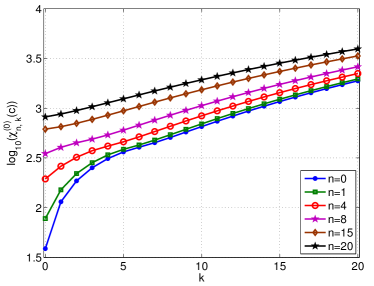
(a) Graph of $\chi_{n,k}^{(0)}(c)$ with $c=20$ and $d=2$.

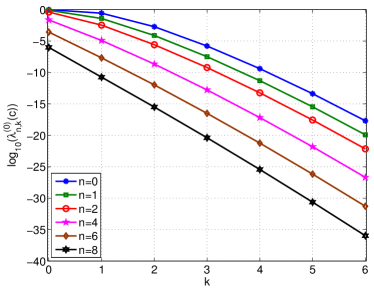
(b) Graph of $\lambda_{n,k}^{(0)}(c)$ with $c=4$ and $d=2$.

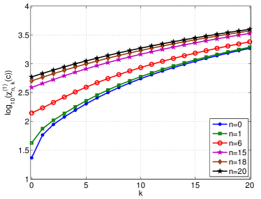
(c) Graph of $\chi_{n,k}^{(1)}(c)$ with $c=10$ and $d=3$.

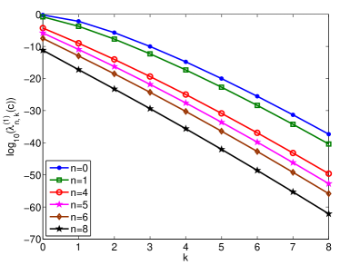
(d) Graph of $\lambda_{n,k}^{(1)}(c)$ with $c=2$ and $d=3$.

Figure 5.1. Graphs of $\chi_{n,k}^{(0)}(c)$ and $\lambda_{n,k}^{(0)}(c).$

In Figure 5.1 (a)-(b), we plot $\chi_{n,k}^{(0)}(c)$ and $\lambda_{n,k}^{(0)}(c)$ versus $k$ in the $2$-dimensional case. It indicates that, for fixed $n$ and $c>0$, $\chi_{n,k}^{(0)}$ becomes larger as $k$ increases, while $\lambda_{n,k}^{(0)}$ decays exponentially as $k$ grows. In Figure 5.2 (a)-(b), we depict the radial component $\psi_{n,k}^{(0)}(r;c)\triangleq r^{n}\phi_{k}^{0,n}(2r^{2}-1;c)$ versus $r\in[0,1.5]$ for $n=0,2,k=0,1,2,3$ and $c=2,10.$ Figures 5.3 -5.4 show surfaces and contours of $\psi_{k,l}^{\alpha,n}(x;c)$ with different $c,k,n$ and $l$ with $d=2,\alpha=0.$

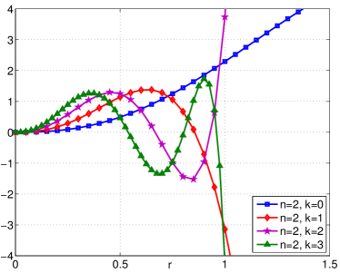
(a) Graph of $\psi_{n,k}^{(0)}(r;c)$ with $c=2$ and $d=2$.

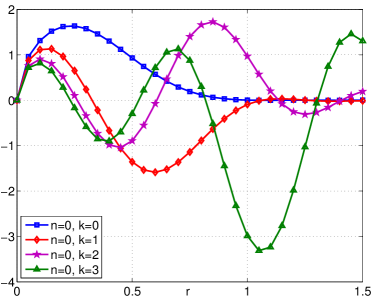
(b) Graph of $\psi_{n,k}^{(0)}(r;c)$ with $c=10$ and $d=2$.

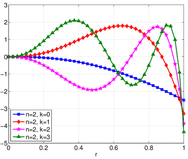
(c) Graph of $\psi_{n,k}^{(0)}(r;c)$ with $c=2$ and $d=3$.

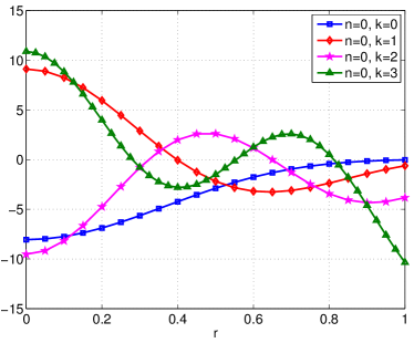
(d) Graph of $\psi_{n,k}^{(1)}(r;c)$ with $c=10$ and $d=3$.

Figure 5.2. Graphs of $\psi_{n,k}^{(\alpha)}(r;c)$ in $2$-dimension and $3$-dimension.

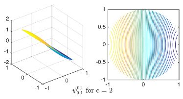
(a) $(\alpha,n,k,l)=(0,1,0,1).$

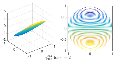
(b) $(\alpha,n,k,l)=(0,1,0,2).$

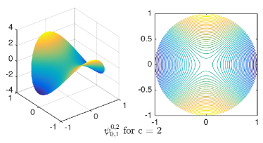
(c) $(\alpha,n,k,l)=(0,2,0,1).$

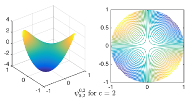
(d) $(\alpha,n,k,l)=(0,2,0,2).$

Figure 5.3. Eigenfunctions $\psi_{k,l}^{\alpha,n}$ with $c=2$ in $2$-dimension.

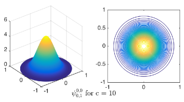
(a) $(\alpha,n,k,l)=(0,0,0,1).$

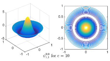
(b) $(\alpha,n,k,l)=(0,0,1,1).$

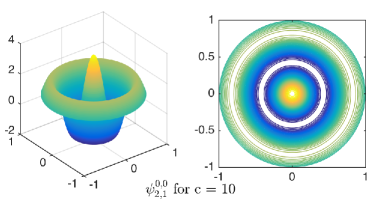
(c) $(\alpha,n,k,l)=(0,0,2,1).$

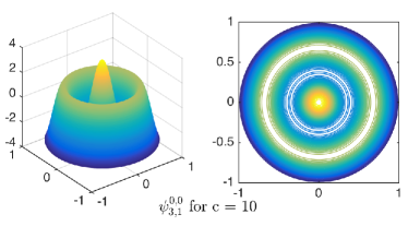
(d) $(\alpha,n,k,l)=(0,0,3,1).$

Figure 5.4. Eigenfunctions $\psi_{k,l}^{\alpha,n}$ with $c=10$ in $2$-dimension.

Table 5.3. The case $d=3$: $\chi_{n,k}^{(1)}(c)$ and $\lambda_{n,k}^{(1)}(c)$

$c$	$n$	$k$	$\chi_{n,k}^{(1)}(c)$	$\lambda_{n,k}^{(1)}(c)$
$0.1$	$0$	$0$	$4.285325573224633e-03$	$1.675003294483135e+00$
$0.5$	$0$	$0$	$1.069001304053325e-01$	$1.662771473208847e+00$
$1$	$0$	$0$	$4.246991437751348e-01$	$1.625460618463697e+00$
$4$	$0$	$0$	$5.948719383823520e+00$	$1.102600593723482e+00$
$10$	$0$	$0$	$2.333891804161449e+01$	$4.186593008319554e-01$
$2$	$1$	$0$	$8.182057327887621e+00$	$4.238871423701353e-01$
$2$	$1$	$1$	$2.609221756616164e+01$	$8.233874011948259e-03$
$2$	$1$	$2$	$5.205150235186056e+01$	$6.516928432939569e-05$
$2$	$1$	$3$	$8.603255633419086e+01$	$2.809367682507114e-07$
$2$	$1$	$4$	$1.280223716202459e+02$	$7.613268689084687e-10$

Table 5.4. The case $d=3:$ $\psi_{n,k}^{(\alpha)}(r;c)\triangleq r^{n}\phi_{k}^{\alpha,n}(2r^{2}-1;c)$ with $\alpha=0,1,2.$

$r$	$c$	$n$	$k$	$\psi_{n,k}^{(0)}(r;c)$	$\psi_{n,k}^{(1)}(r;c)$	$\psi_{n,k}^{(2)}(r;c)$
$0.1$	$1$	$0$	$0$	$\;\;\;5.805625733654062e-01$	$\;\;\;2.820561183868252e+00$	$\;\;\;3.687764193662462e+00$
$0.2$	$1$	$0$	$0$	$\;\;\;8.186066482900428e-01$	$\;\;\;2.814575764166440e+00$	$\;\;\;3.681662607508843e+00$
$0.5$	$1$	$0$	$0$	$\;\;\;1.267632861585855e+00$	$\;\;\;2.772954660597707e+00$	$\;\;\;3.639182765466543e+00$
$1$	$1$	$0$	$0$	$\;\;\;1.662390750491349e+00$	$\;\;\;2.628204021066972e+00$	$\;\;\;3.490731274213273e+00$
$1.3$	$1$	$0$	$0$	$\;\;\;1.765639810965165e+00$	$\;\;\;2.500277467362624e+00$	$\;\;\;3.358563656867405e+00$
$2$	$2$	$0$	$0$	$\;\;\;3.553627999772212e-01$	$\;\;\;8.545596995365403e-01$	$\;\;\;1.510596282792738e+00$
$0.1$	$1$	$2$	$3$	$-1.893124346916359e-01$	$-7.943270542522487e-01$	$-1.008278981214814e+00$
$0.2$	$1$	$2$	$3$	$-8.958937078881810e-01$	$-2.580441975019594e+00$	$-3.177610574908396e+00$
$0.5$	$1$	$2$	$3$	$-1.239366584847178e+00$	$-8.701135484764851e-01$	$\;\;\;3.812964021006710e-01$
$1$	$2$	$2$	$3$	$\;\;\;4.355438266567036e+00$	$\;\;\;2.314178264971302e+01$	$\;\;\;7.372606028015183e+01$
$1.3$	$2$	$2$	$3$	$\;\;\;5.467434735434442e+02$	$\;\;\;1.160117778266639e+03$	$\;\;\;2.449778131304879e+03$
$2$	$2$	$2$	$3$	$\;\;\;4.569351866698169e+04$	$\;\;\;6.922735069954877e+04$	$\;\;\;1.335271987655634e+05$

In Figure 5.1 (c)-(d), we depict that $\chi_{n,k}^{(1)}(c)$ and $\lambda_{n,k}^{(1)}(c)$ for various $k$ in the $3$-dimensional case. It is clear that $\chi_{n,k}^{(1)}(c)$ (resp. $\lambda_{n,k}^{(1)}(c)$) become larger (resp. smaller) as $k$ increases. Some values of $\chi_{n,k}^{(1)}(c)$ and $\lambda_{n,k}^{(1)}(c)$ for a large set of parameter values are given in Table 5.3. We plot in Figure 5.2 (c)-(d) some samples of the $\psi_{n,k}^{(\alpha)}(r;c)$ with $d=3.$ We tabulate some values of $\psi_{n,k}^{(\alpha)}(r;c)$ with $d=3$ in Table 5.4 computed by the aforementioned method. Figures 5.5-5.6 visualize of $\psi_{k,l}^{\alpha,n}(\boldsymbol{x};c)$ with different $k,l,n,\alpha$ and $c$ with $d=3.$

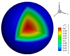
(a) $(\alpha,n,k,l)=(0,0,0,1).$

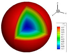
(b) $(\alpha,n,k,l)=(0,0,1,1).$

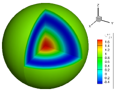
(c) $(\alpha,n,k,l)=(0,0,2,1).$

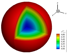
(d) $(\alpha,n,k,l)=(0,2,0,1).$

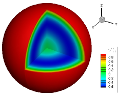
(e) $(\alpha,n,k,l)=(0,2,1,1).$

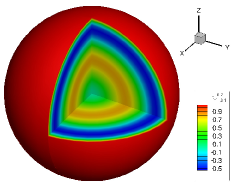
(f) $(\alpha,n,k,l)=(0,2,2,1).$

Figure 5.5. Eigenfunctions $\psi_{k,l}^{\alpha,n}$ with $c=2$ in $3$-dimension.

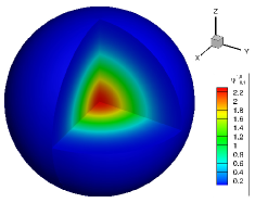
(a) $(\alpha,n,k,l)=(1,0,0,1).$

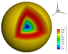
(b) $(\alpha,n,k,l)=(1,0,1,1).$

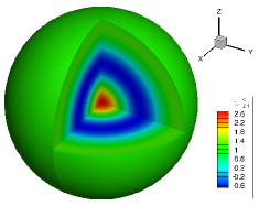
(c) $(\alpha,n,k,l)=(1,0,2,1).$

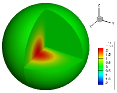
(d) $(\alpha,n,k,l)=(1,1,0,2).$

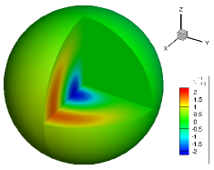
(e) $(\alpha,n,k,l)=(1,1,1,2).$

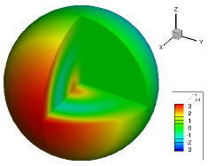
(f) $(\alpha,n,k,l)=(1,1,2,2).$

Figure 5.6. Eigenfunctions $\psi_{k,l}^{\alpha,n}$ with $c=10$ in $3$-dimension.

References

- [1] M. Abramowitz and I. A. Stegun. Handbook of Mathematical Functions. Dover, New York, 1972.
- [2] M.A. Al-Gwaiz. Sturm-Liouville Theory and its Applications. Springer, 2008.
- [3] H. Alici and J. Shen. Highly accurate pseudospectral approximations of the prolate spheroidal wave equation for any bandwidth parameter and zonal wavenumber. J. Sci. Comput., 71(2):1–18, 2016.
- [4] P. Amodio, T. Levitina, G. Settanni, and E.B. Weinmüller. On the calculation of the finite Hankel transform eigenfunctions. J. Appl. Math. Comput., 43(1-2):151–173, 2013.
- [5] G.E. Andrews, R. Askey, and R. Roy. Special Functions. Cambridge University Press, 1999.
- [6] A.P. Bates, Z. Khalid, and R. Kennedy. Efficient computation of slepian functions for arbitrary regions on the sphere. IEEE Trans. Sig. Proc., 65(16):4379–4393, 2016.
- [7] G. Beylkin, C. Kurcz, and L. Monzn. Grids transforms for band-limited functions in a disk. Inverse Problems, 23(5):2059–2088, 2007.
- [8] A. Bonami and A. Karoui. Approximations in Sobolev spaces by prolate spheroidal wave functions. Appl. Comput. Harmon. Anal., 42(3):361–377, 2017.
- [9] M. Botezatu, H. Hult, T.M. Kassaye, and U.G. Fors. Generalized prolate spheroidal wave functions: spectral analysis and approximation of almost band-limited functions. J. Fourier Anal. Appl., 22(2):383–412, 2016.
- [10] C.J. Bouwkamp. On spheroidal wave functions of order zero. Stud. Appl. Math., 26(1-4):79 C92, 1947.
- [11] C.J. Bouwkamp. On the theory of spheroidal wave functions of order zero. Nederl. Akad. Wetensch., Proc., 53:931–944, 1950.
- [12] J.P. Boyd. Large mode number eigenvalues of the prolate spheroidal differential equation. Appl. Math. Comput., 145(2-3):881–886, 2003.
- [13] J.P. Boyd. Algorithm 840: computation of grid points, quadrature weights and derivatives for spectral element methods using prolate spheroidal wave functions—prolate elements. ACM Trans. Math. Software, 31(1):149–165, 2005.
- [14] Q.Y. Chen, D. Gottlieb, and J.S. Hesthaven. Spectral methods based on prolate spheroidal wave functions for hyperbolic PDEs. SIAM J. Numer. Anal., 43(5):1912–1933, 2006.
- [15] E.A. Coddington and N. Levinson. Theory of Ordinary Differential Equations. McGraw-Hill, New York, 1955.
- [16] F. Dai and Y. Xu. Approximation Theory and Harmonic Analysis on Spheres and Balls. Springer-Verlag, 2013.
- [17] C.F. Dunkl and Y. Xu. Orthogonal Polynomials of Several Variables. Cambridge University Press, 2001.
- [18] A. Glaser, X. Liu, and V. Rokhlin. A fast algorithm for the calculation of the roots of special functions. SIAM J. Sci. Comput., 29(4):1420–1438, 2007.
- [19] J.A. Hogan and J.D. Lakey. Duration and Bandwidth Limiting. Applied and Numerical Harmonic Analysis. Birkhäuser/Springer, New York, 2012. Prolate Functions, Sampling, and Applications.
- [20] S. Karnik, Z. Zhu, M.B. Wakin, J. Romberg, and M.A. Davenport. The fast Slepian transform. Appl. Comput. Harmon. Anal., 2017, doi: 10.1016/j.acha.2017.07.005.
- [21] A. Karoui and T. Moumni. New efficient methods of computing the prolate spheroidal wave functions and their corresponding eigenvalues. Appl. Comput. Harmon. Anal., 24(3):269–289, 2008.
- [22] A. Karoui and T. Moumni. Spectral analysis of the finite Hankel transform and circular prolate spheroidal wave functions. J. Comput. Appl. Math., 233(2):315–333, 2009.
- [23] Z. Khalid, R.A. Kennedy, and J.D. McEwen. Slepian spatial-spectral concentration on the ball. Appl. Comput. Harmon. Anal., 40(3):470–504, 2016.
- [24] W.Y. Kong and V. Rokhlin. A new class of highly accurate differentiation schemes based on the prolate spheroidal wave functions. Appl. Comput. Harmon. Anal., 33(2):226–260, 2012.
- [25] B. Landa and Y. Shkolnisky. Approximation scheme for essentially bandlimited and space-concentrated functions on a disk. Appl. Computat. Harmon. Anal., 43(3):381–403, 2017.
- [26] H.J. Landau and H.O. Pollak. Prolate spheroidal wave functions, Fourier analysis and uncertainty-II. Bell System Tech. J., 40(1):65–84, 1961.
- [27] H.J. Landau and H.O. Pollak. Prolate spheroidal wave functions, Fourier analysis and uncertainty-III: The dimension of the space of essentially time- and band-limited signals. Bell System Tech. J., 41(4):1295–1336, 1962.
- [28] R.R. Lederman. Numerical algorithms for the computation of generalized prolate spheroidal functions. ArXiv:1710.0287, 2017.
- [29] V. Michel, S. Orzlowski, and N. Schneider. Vectorial slepian functions on the ball. ArXiv:1707.00425, 2017.
- [30] L. Miranian. Slepian functions on the sphere, generalized gaussian quadrature rule. Inverse Problems, 20(3):877, 2004.
- [31] A. Osipov and V. Rokhlin. On the evaluation of prolate spheroidal wave functions and associated quadrature rules. Appl. Comput.Harmon. Anal., 36(1):108–142, 2014.
- [32] A. Osipov, V. Rokhlin, and H. Xiao. Prolate Spheroidal Wave Functions of Order Zero. Springer, 2013.
- [33] V. Rokhlin and H. Xiao. Approximate formulae for certain prolate spheroidal wave functions valid for large values of both order and band-limit. Appl. Comput. Harmon. Anal., 22(1):105–123, 2007.
- [34] I. Sengupta, B. Sun, W. Jiang, G. Chen, and M.C. Mariani. Concentration problems for bandpass filters in communication theory over disjoint frequency intervals and numerical solutions. J. Fourier Anal. Appl., 18(1):182–210, 2012.
- [35] J. Shen, T. Tang, and L.L. Wang. Spectral Methods: Algorithms, Analysis and Applications. Springer, 2011.
- [36] Y. Shkolnisky. Prolate spheroidal wave functions on a disc-Integration and approximation of two-dimensional bandlimited functions. Appl. Comput. Harmon. Anal., 22(2):235–256, 2007.
- [37] F.J. Simons, F.A. Dahlen, and M.A. Wieczorek. Spatiospectral concentration on a sphere. SIAM Rev., 48(3):504–536, 2006.
- [38] D. Slepian. Prolate spheroidal wave functions, Fourier analysis and uncertainity. IV: Extensions to many dimensions; generalized prolate spheroidal functions. Bell System Tech. J., 43:3009–3057, 1964.
- [39] D. Slepian and H.O. Pollak. Prolate spheroidal wave functions, Fourier analysis and uncertainty. I. Bell System Tech. J., 40(1):43–63, 1961.
- [40] G. Szegö. Orthogonal Polynomials. AMS Coll. Publ., fourth edition, 1975.
- [41] M.A. Taylor and B.A. Wingate. A generalization of prolate spheroidal functions with more uniform resolution to the triangle. J. Engrg. Math., 56(3):221–235, 2006.
- [42] G. Walter and T. Soleski. A new friendly method of computing prolate spheroidal wave functions and wavelets. Appl. Comput. Harmon. Anal., 19(3):432–443, 2005.
- [43] L.L. Wang. A review of prolate spheroidal wave functions from the perspective of spectral methods. J. Math. Study, 50(2):101–143, 2017.
- [44] L.L. Wang and J. Zhang. A new generalization of the PSWFs with applications to spectral approximations on quasi-uniform grids. Appl. Comput. Harmon. Anal., 29(3):303–329, 2010.
- [45] L.L. Wang, J. Zhang, and Z. Zhang. On -convergence of prolate spheroidal wave functions and a new well-conditioned prolate-collocation scheme. J. Comput. Phys., 268:377–398, 2014.
- [46] G.N. Watson. A Treatise on the Theory of Bessel Functions. Cambridge University Press, 1944.
- [47] H. Xiao. Prolate Spheroidal Wave functions, Quadrature, Interpolation, and Asymptotic Formulae. PhD Thesis, Yale University, 2001.
- [48] H. Xiao and V. Rokhlin. High-frequency asymptotic expansions for certain prolate spheroidal wave functions. J. Fourier Anal. Appl., 9(6):575–596, 2003.
- [49] H. Xiao, V. Rokhlin, and N. Yarvin. Prolate spheroidal wavefunctions, quadrature and interpolation. Inverse Problems, 17(4):805–838, 2001. Special issue to celebrate Pierre Sabatier’s 65th birthday (Montpellier, 2000).
- [50] J. Zhang, L.L. Wang, H.Y. Li, and Z. Zhang. Optimal spectral schemes based on generalized prolate spheroidal wave functions of order . J. Sci. Comput., 70(2):451–477, 2017.