Generalized Fitch Graphs: Edge-labeled Graphs that are explained by Edge-labeled Trees

Abstract

Fitch graphs $G=(X,E)$ are di-graphs that are explained by $\{\otimes,1\}$-edge-labeled rooted trees with leaf set $X$: there is an arc $xy\in E$ if and only if the unique path in $T$ that connects the least common ancestor $\operatorname{lca}(x,y)$ of $x$ and $y$ with $y$ contains at least one edge with label “$1$”. In practice, Fitch graphs represent xenology relations, i.e., pairs of genes $x$ and $y$ for which a horizontal gene transfer happened along the path from $\operatorname{lca}(x,y)$ to $y$.

In this contribution, we generalize the concept of Fitch graphs and consider complete di-graphs $K_{|X|}$ with vertex set $X$ and a map $\varepsilon$ that assigns to each arc $xy$ a unique label $\varepsilon(x,y)\in M\cup\{\otimes\}$, where $M$ denotes an arbitrary set of symbols. A di-graph $(K_{|X|},\varepsilon)$ is a generalized Fitch graph if there is an $M\cup\{\otimes\}$-edge-labeled tree $(T,\lambda)$ that can explain $(K_{|X|},\varepsilon)$.

We provide a simple characterization of generalized Fitch graphs $(K_{|X|},\varepsilon)$ and give an $O(|X|^{2})$-time algorithm for their recognition as well as for the reconstruction of the unique least-resolved phylogenetic tree that explains $(K_{|X|},\varepsilon)$.

Keywords: Labeled Gene Trees; Forbidden Subgraphs; Phylogenetics; Xenology; Fitch Graph; Recognition Algorithm

1 Introduction

Edge-labeled graphs that can be explained by vertex-labeled trees have been widely studied and range from cographs [7, 24] and di-cographs [8] to so-called unp-2-structures [14, 15, 16], symbolic ultrametrics [3, 26] or three-way symbolic tree-maps [29, 22]. Besides their structural attractiveness, those types of graphs play an important role in phylogenomics, i.e., the reconstruction of the evolutionary history of genes and species. By way of example, the concept of orthologs, that is, pairs of genes from different species that arose from a speciation event [18], is of fundamental importance in many fields of mathematical and computational biology, including the reconstruction of evolutionary relationships across species [11, 28] or functional genomics and gene organization in species [19, 39]. The orthology relation $\Theta$ is explained by vertex-labeled trees, i.e., a gene pair $(x,y)$ is contained in $\Theta$ if and only if the least common ancestor of $x$ and $y$ is labeled as a speciation event. The graph representation of $\Theta$ must necessarily be a co-graph [24, 3] and provides direct information on the gene history as well as on the history of the species [27, 28]

In contrast, xenology as defined by Walter M. Fitch [17] is explained by edge-labeled rooted phylogenetic trees: a gene $y$ is xenologous with respect to $x$, if and only if the unique path from the least common ancestor $\operatorname{lca}(x,y)$ to $y$ in the gene tree contains a transfer edge. In other words, the xenology relation is explained by an $\{\otimes,1\}$-edge-labeled rooted tree, where an edge with label “$1$” is a transfer edge and an edge with label “$\otimes$” is a non-transfer edge. It has been shown by Geiß et al. [20] that the xenology relation forms a Fitch graph, that is, an $\{\otimes,1\}$-edge-labeled di-graph which is characterized by the absence of eight forbidden subgraphs on three vertices. Moreover, for a given Fitch graph $\mathcal{F}$ it is possible to reconstruct the unique minimally resolved phylogenetic tree that explains $\mathcal{F}$ in linear time.

A further example of graphs and relations that are defined in terms of edge-labeled trees are the single-1-relations $\mathrel{\overset{1}{\sim}}$ and $\mathrel{\overset{1}{\rightharpoonup}}$ [25]. These relations are defined by the existence of a single edge with label “$1$” along the connecting path of two genes and capture the structure of so-called rare genomic changes (RGCs). RGCs have been proven to be phylogenetically informative and helped to resolve many of the phylogenetic questions where sequence data lead to conflicting or equivocal results, see e.g. [4, 9, 12, 13, 30, 31, 32, 33, 37].

In summary, edge-labeled graphs (or equivalently, binary relations) that can be explained by edge-labeled trees provide important information about the evolutionary history of the underlying genes. However, for such type of graphs only few results are available [20, 21, 25].

In this contribution, we extend the notion of xenology and Fitch graphs to generalized Fitch graphs, that is, di-graphs that can be derived from $\{\otimes,1,\dots,m\}$-edge labeled trees, or equivalently, edge-labeled di-graphs that can be explained by such trees. We show that these graphs are characterized by four simple conditions that are defined in terms of edge-disjoint subgraphs. Moreover, we give an $O(|X|^{2})$-time recognition algorithm for generalized Fitch graphs on a set of vertices $X$ and the reconstruction of the unique least-resolved phylogenetic tree that explains them.

2 Preliminaries

2.1 Trees, Di-Graphs and Sets

A rooted tree $T=(V,E)$ (on $X$) is an acyclic connected graphs with leaf set $X$, set of inner vertices $V^{0}=V\setminus X$ and one distinguished inner vertex $\rho_{T}\in V^{0}$ that is called the root of T. In what follows, we consider always phylogenetic trees $T$, that is, rooted trees such that the root $\rho_{T}$ has at least degree $2$ and every other inner vertex $v\in V^{0}\setminus\{\rho_{T}\}$ has at least degree $3$.

We call $u\in V$ an ancestor of $v\in V$, $u\succeq_{T}v$, and $v$ a descendant of $u$, $v\preceq_{T}u$, if $u$ lies on the unique path from $\rho_{T}$ to $v$. We write $v\prec_{T}u$ ($u\succ_{T}v$) for $v\preceq_{T}u$ ($u\succeq_{T}v$) and $u\neq v$. Edges that are incident to a leaf are called outer edges. Conversely, inner edges do only contain inner vertices. For a non-empty subset $Y\subseteq X$ of leaves, the least common ancestor of $Y$, denoted as $\operatorname{lca}_{T}(Y)$, is the unique $\preceq_{T}$-minimal vertex of $T$ that is an ancestor of every vertex in $Y$. We will make use of the simplified notation $\operatorname{lca}_{T}(x,y):=\operatorname{lca}_{T}(\{x,y\})$ for $Y=\{x,y\}$ and we will omit the explicit reference to $T$ whenever it is clear which tree is considered. For a subset $Y\subseteq X$ of leaves, the tree $T(Y)$ with root $\operatorname{lca}_{T}(Y)$ has leaf set $Y$ and consists of all paths in $T$ that connect the leaves in $Y$. The restriction $T_{|Y}$ of $T$ to some subset $Y\subseteq X$ is the rooted tree obtained from $T(Y)$ by suppressing all vertices of degree $2$ with the exception of the root $\rho_{T}$ if $\rho_{T}\in V(T(Y))$.

A contraction of an edge $e=xy$ in a tree $T$ refers to the removal of $e$ and identification of $x$ and $y$. We say that a rooted tree $T$ on $L$ displays a root tree $T^{\prime}$ on $L^{\prime}$, in symbols $T^{\prime}\leq T$, if $T^{\prime}$ can be obtained from $T(L^{\prime})$ by a sequence of edge contractions. If $T^{\prime}\leq T$, then we also say that $T$ refines $T^{\prime}$.

Rooted triples are binary rooted phylogenetic trees on three leaves. We write $ab|c$ for the rooted triple with leaves $a,b$ and $c$, if the path from its root to $c$ does not intersect the path from $a$ to $b$. The definition of “display” implies that a triple $ab|c$ with $a,b,c\in L$ is displayed by a rooted tree $T$ if $\operatorname{lca}(a,b)\prec_{T}\operatorname{lca}(a,b,c)$. The set of all triples that are displayed by $T$ is denoted by $r(T)$. A set of rooted triples $R$ is called consistent if there exists a phylogenetic tree $T$ on $L_{R}\coloneqq\bigcup_{ab|c\in R}\{a,b,c\}$ that displays $R$, i.e., $R\subseteq r(T)$. As shown in [1] there is a polynomial-time algorithm, usually referred to as BUILD [36, 38], that takes a set $R$ of triples as input and either returns a particular phylogenetic tree $\operatorname{Aho}(R)$ that displays $R$, or recognizes $R$ as inconsistent.

A set of rooted triples $R$ identifies a tree $T$ with leaf set $L_{R}$ if $R$ is displayed by $T$ and every other tree $T^{\prime}$ that displays $R$ is a refinement of $T$. A rooted triple $ab|c\in r(T)$ distinguishes an edge $uv$ in $T$ iff $a$, $b$, and $c$ are descendants of $u$; $v$ is an ancestor of $a$ and $b$ but not of $c$; and there is no descendant $v^{\prime}$ of $v$ for which $a$ and $b$ are both descendants. In other words, $ab|c\in r(T)$ distinguishes the edge $uv$ if $\operatorname{lca}(a,b)=v$ and $\operatorname{lca}(a,b,c)=u$.

The requirement that a set $R$ of triples is consistent, and thus, that there is a tree displaying all triples, makes it possible to infer new triples from the trees that display $R$ and to define a closure operation for $R$ [23, 6, 34, 5]. Let $\langle R\rangle$ be the set of all rooted trees with leaf set $L_{R}$ that display $R$. The closure of a consistent set of rooted triples $R$ is defined as

$$\operatorname{cl}(R)=\bigcap_{T\in\langle R\rangle}r(T).$$

Hence, a triple $r$ is contained in the closure $\operatorname{cl}(R)$ if all trees that display $R$ also display $r$. This operation satisfies the usual three properties of a closure operator [6], namely: (i) expansiveness, $R\subseteq\operatorname{cl}(R)$; (ii) isotony, $R^{\prime}\subseteq R$ implies that $\operatorname{cl}(R^{\prime})\subseteq\operatorname{cl}(R)$; and (iii) idempotency, $\operatorname{cl}(\operatorname{cl}(R))=\operatorname{cl}(R)$. Since $T\in\langle r(T)\rangle$, it is easy to see that $\operatorname{cl}(r(T))=r(T)$ and thus, $r(T)$ is always closed.

For later reference , we give here an important result from [23] that is closely related to the BUILD algorithm.

Lemma 2.1.

Let $T$ be a phylogenetic tree and let $R$ be a set of rooted triples. Then, $R$ identifies $T$ if and only if $\operatorname{cl}(R)=r(T)$. Moreover, if $R$ identifies $T$, then $\operatorname{Aho}(R)=T$.

In this contribution, we will consider phylogenetic trees $T=(V,E)$ together with an edge-labeling map $\lambda:E\to M\cup\{\otimes\}$, where $M=\{1,\dots|M|\}$ denotes a non-empty set of symbols and we write $(T,\lambda)$. Edges that have label $m\in M\cup\{\otimes\}$ are called $m$-edges. Furthermore, $M^{\otimes}$ will always denote the set $M\cup\{\otimes\}$.

For a di-graph $G=(V,E)$ and a subset $W\subseteq V$ we denote with $G[W]=(W,F)$ the induced subgraph of $G$, i.e., any arc $xy\in E$ with $x,y\in W$ is also contained in $G[W]$.

In what follows, $[X\times X]_{\textrm{irr}}$ denotes the set $(X\times X)\setminus\{(x,x)\mid x\in X\}$. To avoid trivial cases, we always assume that $|X|>1$. The sets $X_{1},\dots,X_{k}$ form a quasi-partition of $X$, if all sets are pairwisely disjoint, their union is $X$ and at most one $X_{i}$ is empty.

2.2 Simple Fitch Graphs

Let $\lambda:E\to\{1,\otimes\}$ be a map and $(T,\lambda)$ be an edge-labeled phylogenetic tree on $X$. We set $(x,y)\in\mathcal{X}_{(T,\lambda)}$ for $x,y\in X$ whenever the uniquely defined path from $\operatorname{lca}_{T}(x,y)$ to $y$ contains at least one 1-edge. By construction $\mathcal{X}_{(T,\lambda)}$ is irreflexive; hence it can be regarded as a simple directed graph.

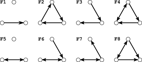
An arbitrary di-graph $G=(X,E)$ is explained by a phylogenetic tree $(T,\lambda)$ (on $X$) and called simple Fitch graph, whenever $xy\in E$ if and only if $(x,y)\in\mathcal{X}_{(T,\lambda)}$. Fitch graphs are the topic of Ref. [20], which among other results gave a characterization in terms of eight forbidden induced subgraphs. The following theorem summarizes a couple of important results that we need for later reference.

Theorem 2.2 ([20]).

A given di-graph $G=(X,E)$ is a simple Fitch graph if and only if it does not contain one the graphs $F_{1},\dots,F_{8}$ (shown in Fig. 1) as an induced subgraph.

Deciding whether $G$ is a simple Fitch graph and, in the positive case, to construct the unique least-resolved tree $(T,\lambda)$ that explains $G$ can be done in $O(|X|+|E|)$ time.

$(T,\lambda)$ is a least-resolved tree that explains $G$, i.e., there is no edge-contracted version $T^{\prime}$ of $T$ and no labeling $\lambda^{\prime}$ such that $(T^{\prime},\lambda^{\prime})$ still explains $G$, if and only if all its inner edges are 1-edges and for every inner edge $(u,v)$ there is an outer $\otimes$-edge $(v,x)$ in $(T,\lambda)$.

Figure 1: Shown are the eight forbidden induced subgraphs $F_{1},\dots,F_{8}$ of Fitch graphs.

3 Generalized Fitch Graphs

To generalize the notion of simple Fitch graphs, we consider complete di-graphs $(K_{|X|},\varepsilon)$ with vertex $X$, arc set $[X\times X]_{\textrm{irr}}$ and a map $\varepsilon:[X\times X]_{\textrm{irr}}\to M^{\otimes}$ that assigns to each arc $xy$ a unique label $\varepsilon(x,y)$. Clearly, the map $\varepsilon$ covers all information provided by $(K_{|X|},\varepsilon)$. W.l.o.g. we will always assume that for each $m\in M$ there is at least one pair $(x,y)\in[X\times X]_{\textrm{irr}}$ such that $\varepsilon(x,y)=m$.

Definition 3.1.

Let $\varepsilon:[X\times X]_{\textrm{irr}}\to M^{\otimes}$ be a map. For a given phylogenetic tree $(T,\lambda)$ with $\lambda:E\to M^{\otimes}$ and two leaves $x$ and $y$ we denote with $\mathbb{P}_{(x,y)}$ the unique path in $T$ from $\operatorname{lca}_{T}(x,y)$ to $y$. A pair $(x,y)\in[X\times X]_{\textrm{irr}}$ is explained by a phylogenetic tree $(T,\lambda)$ on $X$ whenever,

$\varepsilon(x,y)=m\in M$ iff some edge $e$ on the path $\mathbb{P}_{(x,y)}$ has label $\lambda(e)=m$; and

$\varepsilon(x,y)=\otimes$ iff none of the edges $e$ on the path $\mathbb{P}_{(x,y)}$ have label $\lambda(e)\in M$.

The map $\varepsilon$ is tree-like if each pair $(x,y)\in[X\times X]_{\textrm{irr}}$ is explained by $(T,\lambda)$. In this case, we say that $(T,\lambda)$ explains $\varepsilon$ and $(K_{|X|},\varepsilon)$ is a (generalized) Fitch graph.

Moreover, a tree $(T,\lambda)$ is least-resolved for a map $\varepsilon$, if $(T,\lambda)$ explains $\varepsilon$ and there is no tree $(T^{\prime},\lambda^{\prime})$ that explains $\varepsilon$, where $T^{\prime}$ is obtained from $T$ by contracting edges and $\lambda^{\prime}$ is an $M\cup\{\otimes\}$-edge-labeling map.

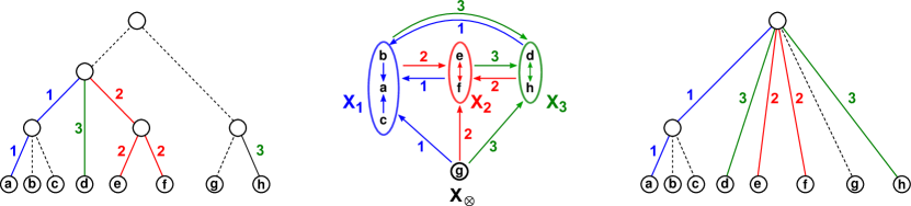
Figure 3 shows an example of a generalized Fitch graph $(K_{|X|},\varepsilon)$. We give the following almost trivial result for later reference.

Lemma 3.2.

Let $\varepsilon:[X\times X]_{\textrm{irr}}\to M^{\otimes}$ be tree-like and $(T,\lambda)$ be a tree that explains $\varepsilon$. If there is an edge $e$ with $\lambda(e)=m$ on the path $P$ from the root $\rho_{T}$ to some leaf, then all edges in $P$ are either labeled with $m$ or $\otimes$.

Proof.

Let $P$ be the path from the root $\rho_{T}$ to the leaf $x\in X$. Let $v$ be the child of $\rho_{T}$ that is an ancestor of $x$. Now let $y\in X$ be any leaf that is not a descendant of $v$ and thus $\operatorname{lca}_{T}(x,y)=\rho_{T}$. Assume, for contradiction, that there are two edges in $P$ with distinct labels $m,m^{\prime}\in M$. Since $(T,\lambda)$ explains $\varepsilon$ we would have $\varepsilon(y,x)=m$ and $\varepsilon(y,x)=m^{\prime}$; a contradiction to $\varepsilon$ being a map. ∎

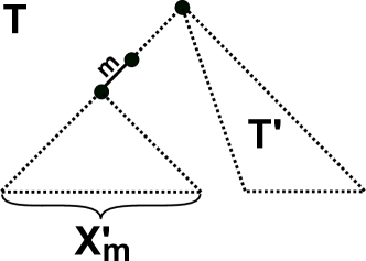
For each symbol $s\in M^{\otimes}$ we define the following set

$$X_{s}\coloneqq\{x\in X\mid \text{ there is a vertex }z\in X\text{ with }\varepsilon(z,x)=s$$

$$\text{ and for all }z^{\prime}\in X\setminus\{z,x\}\text{ we have }\varepsilon(z^{\prime},x)\in\{\otimes,s\}\}$$

that contains for each symbol $s$ those vertices $x\in X$ where at least one incoming arc is labeled $s$ and all other incoming arcs have label $s$ or $\otimes$. Note, by construction for all $x,y\in X_{\otimes}$ we have $\varepsilon(x,y)=\varepsilon(y,x)=\otimes$ and for all $x,y\in X_{m}$, $m\in M$ we have $\varepsilon(x,y),\varepsilon(y,x)\in\{m,\otimes\}$.

The intuition behind the sets $X_{s}$ is sketched in Fig. 2. In this example, let $(K_{|X|},\varepsilon)$ be the Fitch graph that is explained by the sketched tree and assume that the highlighted $m$-edge $e$ with $m\neq\otimes$ is the first $m$-edge that lies on the path from the root to any of the leaves that are located below this edge. Lemma 3.2 implies that all edges on this path that are above $e$ must be $\otimes$-edges and all edges below $e$ must either be $\otimes$- or $m$-edges. This observation implies that every leaf $z$ located in the subtree $T^{\prime}$ must “point to” to every leaf $x\in X^{\prime}_{m}$ via an $m$-edge in $(K_{|X|},\varepsilon)$, i.e., $\varepsilon(z,x)=m$. Moreover, for any two vertices $z^{\prime},x\in X^{\prime}_{m}$ we have $\varepsilon(z^{\prime},x)\in\{\otimes,m\}$. Thus, the set $X^{\prime}_{m}$ in Fig. 2 is a subset of the (possibly larger) set $X_{m}$.

Figure 2: Shown is a sketched tree $T$, where the highlighted $m$-edge $e$ is the first $m$-edge that is located on the path from the root to any of the leaves below $e$. Thus, $X^{\prime}_{m}\subseteq X_{m}$, see text for further details.

Lemma 3.3.

Let $\varepsilon:[X\times X]_{\textrm{irr}}\to M^{\otimes}$ be a tree-like map and $(T,\lambda)$ a tree that explains $\varepsilon$. Then, for all $m\in M$ we have $X_{m}\neq\emptyset$ and $X_{m}=\{x\in X\mid\exists z\in X\text{ with }\varepsilon(z,x)=m\}$. In particular, the sets $X_{1},X_{2},\dots X_{|M|},X_{\otimes}$ form a quasi-partition of $X$.

Moreover, for all $x\in X_{m}$ and $y\in X\setminus X_{m}$ with $m\in M^{\otimes}$ it holds that $\varepsilon(y,x)=m$.

Proof.

To recap, $\varepsilon$ is a map such that $\varepsilon^{-1}(m)\neq\emptyset$ for all $m\in M$. Thus, for each $m\in M$ there are two vertices $x,z\in X$ with $\varepsilon(z,x)=m$. Assume for contradiction that there is a vertex $z^{\prime}\in X$ with $\varepsilon(z^{\prime},x)=m^{\prime}\notin\{m,\otimes\}$. Thus, the path from $\operatorname{lca}(z,x)$ to $x$ contains an edge labeled $m$ and the path from $\operatorname{lca}(z^{\prime},x)$ to $x$ contains an edge labeled $m^{\prime}$. However, since both vertices $\operatorname{lca}(x,z)$ and $\operatorname{lca}(x,z^{\prime})$ are located on the path from the root of $T$ to $x$, this path must have two edges, one with label $m$ and one with label $m^{\prime}$; a contradiction to Lemma 3.2. Thus, $\varepsilon(z,x)\in\{m,\otimes\}$ for all $z\in X\setminus\{x\}$ and therefore, $x\in X_{m}$. Thus, $X_{m}\neq\emptyset$ for all $m\in M$. In particular, the latter arguments imply that whenever there are vertices $x,z\in X$ with $\varepsilon(z,x)=m$, then for all vertices $z^{\prime}\in X\setminus\{x\}$ we have $\varepsilon(z^{\prime},x)\in\{m,\otimes\}$ and thus, the sets $X_{m}$ and $\{x\in X\mid\exists z\in X\text{ with }\varepsilon(z,x)=m\}$ are identical.

We continue to show that $X_{1},X_{2},\dots X_{|M|},X_{\otimes}$ form a quasi-partition of $X$. Clearly, for all distinct $m,m^{\prime}\in M$ the sets $X_{m},X_{m^{\prime}}$ must be disjoint, as otherwise $x\in X_{m}\cap X_{m^{\prime}}$ would imply that $\varepsilon(z,x)=m$ for some $z\in X$ and at the same time $\varepsilon(z,x)\in\{m^{\prime},\otimes\}$; a contradiction to $\varepsilon$ being a map. Moreover, for all distinct $m\in M$ the sets $X_{m},X_{\otimes}$ must be disjoint, since $x\in X_{\otimes}$ if and only if $\varepsilon(z,x)=\otimes$ for all $z\in X\setminus\{x\}$, which is, if and only if $x\notin X_{m}$ for all $m\in M$.

It remains to show that the union of $X_{1},X_{2},\dots X_{|M|},X_{\otimes}$ is $X$ and at most one of the sets is empty. Note, for each $m\in M$ there are two vertices $z,x\in X$ with $\varepsilon(z,x)=m$. As argued above, $\varepsilon(z,x)=m\in M$ implies $x\in X_{m}$. Thus, none of the sets $X_{1},X_{2},\dots X_{|M|}$ is empty. In particular, $X_{\otimes}=\emptyset$ if and only if for every $x\in X$ we have $\varepsilon(z,x)=m$ for some $z\in X$ and $m\in M$. In this case, the union of the sets $X_{1},X_{2},\dots X_{|M|}$ is $X$. Now assume that $X_{\otimes}\neq\emptyset$ and $x\notin X_{m},m\in M$. Hence, $\varepsilon(z,x)\neq m$ for all $z\in X\setminus\{x\}$ and all $m\in M$. Thus, $\varepsilon(z,x)=\otimes$ for all $z\in X\setminus\{x\}$, and therefore, $x\in X_{\otimes}$. Thus, in case $X_{\otimes}\neq\emptyset$, the union of the sets $X_{1},X_{2},\dots X_{|M|},X_{\otimes}$ is $X$.

To prove the last statement, let $x\in X_{m}$. Clearly, if $m=\otimes$ and thus, $x\in X_{\otimes}$ then $\varepsilon(y,x)=\otimes$ for all $y\in X\setminus\{x\}$. Now, let $m\in M$ and $m^{\prime}\in M^{\otimes}$ with $m\neq m^{\prime}$. Assume for contradiction that $\varepsilon(y,x)\neq m$ for some $y\in X_{m^{\prime}}$. Thus, the path from $\operatorname{lca}(x,y)$ to $x$ does not contain an $m$-edge. By construction of $X_{m}$, there is a vertex $z\in X$ with $\varepsilon(z,x)=m$ and thus, the path from $\operatorname{lca}(x,z)$ to $x$ contains an $m$-edge $e=uv$. Trivially, all ancestors of $x$ are located on the path from the root of $T$ to $x$ and thus, also $\operatorname{lca}(x,z)$ and $\operatorname{lca}(x,y)$. Therefore, the $m$-edge is located between $\operatorname{lca}(x,z)$ and $\operatorname{lca}(x,y)$ and, in particular, $\operatorname{lca}(x,z)\succeq u\succ v\succeq\operatorname{lca}(x,y)$. Hence, $\operatorname{lca}(x,z)=\operatorname{lca}(y,z)$ and the path from $\operatorname{lca}(y,z)$ to $z$ contains an $m$-edge; a contradiction to $y\in X_{m^{\prime}}$. ∎

Figure 3: Left, an edge-labeled tree $(T,\lambda)$ is shown where $\otimes$-edges are drawn as dashed-lines. The tree $(T,\lambda)$ explains the graph $(K_{|X|},\varepsilon)$ in the middle, where $X=\{a,b,\dots,h\}$ and $\varepsilon:[X\times X]_{\textrm{irr}}\to\{1,2,3,\otimes\}$. For better readability, $\otimes$-edges are omitted in the drawing of $(K_{|X|},\varepsilon)$ and only one arc $xy$ with label $\varepsilon(x,y)=m^{\prime}$ and $\varepsilon(y,x)=m$ for each $x\in X_{m}$ and $y\in X_{m^{\prime}}$, $m\neq m^{\prime}$ is drawn. All arcs between vertices $x,y\in X_{m}$ have label $m$. The least-resolved tree $(T^{*},\lambda^{*})$ constructed with Alg. 2 is shown at the right-hand side.

For each $m\in M$, we denote with $G_{m}$ the subgraph of $(K_{|X|},\varepsilon)$ with vertex set $X_{m}$ as defined above and arc set

$$E_{m}=\{xy\mid x,y\in X_{m},\varepsilon(xy)\neq\otimes\}.$$

Note, by definition of $X_{m}$, the graph $G_{m}$ contains only arcs $xy$ with $\varepsilon(xy)=m$.

Before we can derive the final result, we need one further definition. Let $(T,\lambda)$ be an edge-labeled phylogenetic tree on $X$. To recap, the restriction $T_{|X_{m}}$ of $T$ to $X_{m}$ is obtained by suppressing all degree-$2$ vertices of $T(X_{m})$. For any edge $uv\in E(T_{|X_{m}})$, let $S(u,v)$ denote the set of all suppressed vertices on the path from $u$ to $v$ in $T(X_{m})$. We define the restriction $\lambda_{|X_{m}}$ to $X_{m}$ by putting for all edges $uv\in E(T_{|X_{m}})$:

$$\lambda_{|X_{m}}(x,y)=\begin{cases}\lambda(u,v)&\,\text{, if }S(u,v)=\emptyset\text{ and thus, }uv\in E(T)\\ m&\,\text{, else if }\text{there are }a,b\in S(u,v)\cup\{u,v\}\text{ with }\lambda(a,b)=m\\ \otimes&\,\text{, else.}\end{cases}$$

Lemma 3.2 implies that the restriction $\lambda_{|X_{m}}$ of $\lambda$ is well defined. In particular, $\lambda_{|X_{m}}(u,v)=m$ if and only if the corresponding unique path between $u$ and $v$ in $T$ contains an $m$-edge.

We are now in the position to characterize tree-like maps $\varepsilon$.

Theorem 3.4.

The map $\varepsilon:[X\times X]_{\textrm{irr}}\to M^{\otimes}$ is tree-like (or equivalently $(K_{|X|},\varepsilon)$ is a generalized Fitch graph) if and only if the following four conditions are satisfied:

(T1)

The sets $X_{1},X_{2},\dots X_{|M|},X_{\otimes}$ form a quasi-partition of $X$.

(T2)

$G_{m}=(X_{m},E_{m})$ is a simple Fitch graph for all $m\in M$.

(T3)

For all $m\in M$ and $x\in X_{m}$, $y\in X\setminus X_{m}$ it holds that $\varepsilon(y,x)=m$.

(T4)

For all $x\in X_{\otimes}$ and $y\in X\setminus\{x\}$ it holds that $\varepsilon(y,x)=\otimes$.

In particular, the tree $(T^{*},\lambda^{*})$ returned by Algorithm 2 (with input $\varepsilon$) explains $\varepsilon$, whenever $\varepsilon$ is tree-like.

Proof.

We first establish the ‘if’ direction. Assume Conditions (T1) to (T4) are satisfied for $\varepsilon$. Since $G_{m}=(X_{m},E_{m})$ is a simple Fitch graph for all $m\in M$, all $G_{m}$ are explained by a tree $(T_{m},\lambda_{m})$ with leaf set $X_{m}$.

We show that the tree $(T^{*},\lambda^{*})$ constructed with Alg. 2 explains $\varepsilon$. By construction of $(T^{*},\lambda^{*})$ all trees $(T_{m},\lambda_{m})$ are exactly the subtrees $T^{*}(X_{m})$ where all edge labels $\lambda_{m}$ are kept. Hence, $G_{m}$ is explained by $(T^{*}(X_{m}),\lambda^{*}_{|X_{M}})$. Since $\varepsilon(x,y)=m$ (resp. $\varepsilon(x,y)=\otimes$) for any $x,y\in X_{m}$ if and only if $xy\in E_{m}$ (resp. $xy\not\in E_{m}$), we can conclude that all pairs $(x,y),(y,x)$ with $x,y\in X_{m}$ are explained by $(T^{*},\lambda^{*})$ for all $m\in M$. Moreover, each $x\in X_{\otimes}$ is linked to the root $\rho_{T^{*}}$ via an $\otimes$-edge (Line 11 of Alg. 2). Hence, for each two vertices $x,y\in X_{\otimes}$ we have, by definition of $X_{\otimes}$, $\varepsilon(x,y)=\varepsilon(y,x)=\otimes$, which is trivially explained by $(T^{*},\lambda^{*})$. Since the sets $X_{1},X_{2},\dots X_{|M|},X_{\otimes}$ form a quasi-partition of $X$, it is ensured that there are no overlapping leaf sets when the trees $(T_{m},\lambda_{m})$ and the elements $x\in X_{\otimes}$ have been added to $(T^{*},\lambda^{*})$ and that the leaf set of $T^{*}$ is $X$.

We continue to show that all pairs $(x,y)$ with $x,y\in X$ that satisfy (T3) and (T4) are explained by $(T^{*},\lambda^{*})$. Note first, by construction of $(T^{*},\lambda^{*})$ and since $(T^{*},\lambda^{*})$ explains $G_{m}$ for all $m\in M$, all edges along the path from $\rho_{T^{*}}$ to $x\in X_{m}$ have label $m$ or $\otimes$. Even more, we show that each path $P_{\rho_{T^{*}},x}$ from $\rho_{T^{*}}$ to each $x\in X_{m}$, $m\in M$ has always an edge with label $m$. By construction of $(T^{*},\lambda^{*})$ (Alg. 2, Line 6-8), if $|X_{m}|=1$ or there is a leaf $x\in X_{m}$ adjacent to the root $\rho_{m}$ of $T_{m}$ such that $\lambda_{m}(\rho_{m},x)=\otimes$, then the tree $(T_{m},\lambda_{m})$ is placed below the particular $m$-edge $\rho_{T^{*}}r_{m}$. Hence, all paths from $\rho_{T^{*}}$ to $x\in X_{m}$ contain this $m$-edge. Since (T3) and (T4) state that $\varepsilon(y,x)=m$ for all $x\in X_{m}$, $m\in M$, all pairs $(y,x)$ with $x\in X_{m}$, $y\in X\setminus X_{m}$ are explained by $(T^{*},\lambda^{*})$, given that $(T_{m},\lambda_{m})$ satisfies the Conditions in Alg. 2 (Line 6). Assume that $(T_{m},\lambda_{m})$ does not satisfy the latter conditions. Theorem 2.2 implies that all inner edges of $(T_{m},\lambda_{m})$ are $m$-edges and thus, any $\otimes$-edge in $(T_{m},\lambda_{m})$ must be incident to some leaf $x\in X_{m}$. Since $(T_{m},\lambda_{m})$ does not satisfy the if-condition in Line 6 of Alg. 2, all edges that are incident to the root of $(T_{m},\lambda_{m})$ have label $m$. Hence, all paths from $\rho_{T^{*}}$ to $x\in X_{m}$ contain an $m$-edge and, therefore, all pairs $(y,x)$ with $x\in X_{m}$, $y\in X\setminus X_{m}$ are explained by $(T^{*},\lambda^{*})$. Finally, if $x\in X_{\otimes}$, then (T4) claims $\varepsilon(y,x)=\otimes$ for all $y\neq x$ which is trivially explained by $(T^{*},\lambda^{*})$, since $x$ is linked to the root $\rho_{T^{*}}$ via an $\otimes$-edge (Alg. 2, Line 11). In summary, if the Conditions (T1) to (T4) are satisfied, then $\varepsilon$ is explained by $(T^{*},\lambda^{*})$ and therefore, tree-like. This establishes the ‘if’ direction.

We turn now to the ‘only if’ direction. Assume that $\varepsilon$ is tree-like and let $(T,\lambda)$ be a tree that explains $\varepsilon$ with root $\rho_{T}$. Lemma 3.3 implies Condition (T1), (T3) and (T4). We continue to show (T2). To this end, consider the graph $G_{m}=(X_{m},E_{m})$, $m\in M$. Since $(T,\lambda)$ explains $\varepsilon$ and therefore, also $(K_{|X|},\varepsilon)$, it must explain each of its induced subgraphs and thus, any pair $(x,y)$ with $x,y\in X_{m}$ and $m\in M$ is explained by $(T,\lambda)$. By construction of the restriction $(T_{|X_{m}},\lambda_{|X_{m}})$ of $(T,\lambda)$ to $X_{m}$ we have $\varepsilon(x,y)=m$ if and only if the path in $(T,\lambda)$ from $\operatorname{lca}_{T}(x,y)$ to $y$ contains an $m$-edge which is if and only if there is an $m$-edge on the path from $\operatorname{lca}_{T_{|X_{m}}}(x,y)$ to the leaf $y$ in $(T_{|X_{m}},\lambda_{|X_{m}})$. Hence, $(T_{|X_{m}},\lambda_{|X_{m}})$ explains $(K_{|X|}[X_{M}],\varepsilon)$. By definition of $X_{m}$, the graph $G_{m}$ contains only arcs $xy$ with $\varepsilon(x,y)=m$ and for all $x,y\in X_{m}$ with $xy\notin E_{m}$ we have $\varepsilon(x,y)=\otimes$. Thus, $G_{m}$ is obtained from $(K_{|X|}[X_{M}],\varepsilon)$ by removing all $\otimes$-edges and is, therefore, explained by $(T_{|X_{m}},\lambda_{|X_{m}})$. Hence, $G_{m}$ is a simple Fitch graph and (T2) is satisfied. This establishes the ‘only if’ direction.

Thus, Conditions (T1) to (T4) characterize tree-like maps $\varepsilon$. This together with the proof of the ‘if’ direction implies the correctness of Alg. 2. ∎

Algorithm 1 Recognition of tree-like maps $\varepsilon$.

1:A map $\varepsilon:[X\times X]_{\textrm{irr}}\to M^{\otimes}$;

2:A least-resolved edge-labeled tree $(T^{*},\lambda^{*})$ that explains $\varepsilon$ or the statement “The map $\varepsilon$ is not tree-like”;

3:if $|M|>2|X|-2$ then Output: “The map $\varepsilon$ is not tree-like”;

4:else if  $\varepsilon$ satisfies Condition (T1) to (T4) in Thm. 3.4  then

5:    Compute $(T^{*},\lambda^{*})$ with Alg. 2;

6:else Output: “The map $\varepsilon$ is not tree-like”;

Algorithm 2 Compute Least-Resolved Tree $(T^{*},\lambda^{*})$ for $\varepsilon$.

1:A tree-like map $\varepsilon:[X\times X]_{\textrm{irr}}\to M^{\otimes}$;

2:A least-resolved edge-labeled tree $(T^{*},\lambda^{*})$ that explains $\varepsilon$;

3:Add a root $\rho_{T^{*}}$ to $T^{*}$;

4:for all $m\in M$ do

5:    Compute the least-resolved tree $(T_{m},\lambda_{m})$ the explains $G_{m}=(X_{m},E_{m})$;

6:    if $|X_{m}|=1$ OR $(T_{m},\lambda_{m})$ contains an $\otimes$-edge incident to its root then

7:        Add a vertex $r_{m}$ and the edge $\rho_{T^{*}}r_{m}$ with label $m$;

8:        Add $(T_{m},\lambda_{m})$ by identifying the root of $T_{m}$ with $r_{m}$;

9:        Set $\lambda^{*}(e)=\lambda_{m}(e)$ for all edges in $T_{m}$;

10:    else Identify the root of $T_{m}$ with $\rho_{T^{*}}$ and add $(T_{m},\lambda_{m})$;     

11:Add an edge $e=\rho_{T^{*}}x$ with label $\lambda^{*}(e)=\otimes$ for all $x\in X_{\otimes}$;

12:Return $(T^{*},\lambda^{*})$;

Theorem 3.5.

For a given map $\varepsilon:[X\times X]_{\textrm{irr}}\to M^{\otimes}$, Algorithm 1 determines whether $\varepsilon$ is tree-like or not, and returns a tree $(T^{*},\lambda^{*})$ that explains a tree-like map $\varepsilon$ in $O(|X|^{2})$-time.

In particular, if $\varepsilon$ is tree-like, then $(T^{*},\lambda^{*})$ is a least-resolved tree for $\varepsilon$.

Proof.

To establish the correctness of Alg.  1, note first that for any tree $T=(V,E)$ on $X$ we have $|E|+1=|V|\leq 2|X|-1$ (cf. [28, Lemma 1]). Thus, there is no tree with $|E|>2|X|-2$ edges and hence, one can place at most $2|X|-1$ different symbols on the edges of a tree. Therefore, if $|M|>2|X|-2$, then $\varepsilon$ cannot be tree-like, since we claimed that for any $m\in M$, $\varepsilon^{-1}(m)\neq\emptyset$. This establishes the correctness of Line 3 of Alg. 1. Now, apply Thm. 3.4 to conclude that Alg. 1 is correct.

We continue to verify the runtime of Alg.  1. Clearly, the sets $X_{1},\dots,X_{|M|},X_{\otimes}$ can be constructed by stepwisely considering each pair $(x,y)\in[X\times X]_{\textrm{irr}}$ and its label $\varepsilon(x,y)$, which takes $O(|X|^{2})$-time. In particular, verifying Condition (T1) can be done directly within the construction phase of the sets $X_{m}$, $m\in M^{\otimes}$ and, hence stays within the time complexity of $O(|X|^{2})$. Thm. 2.2 implies that Condition (T2) can be verified in $O(|X|+|E_{m}|)$ time for each $m\in M$. Due to the ‘if-condition’ in Line 3 of Alg. 1, we have $|M|\in O(|X|)$. Furthermore, $\sum_{m\in M}E_{m}\in O(|X|^{2})$. Thus, Condition (T2) can be checked in $\sum_{m\in M}O(|X|+|E_{m}|)=O(|M||X|)+|X|^{2})=O(|X|^{2})$ time. Finally, for (T3) and (T4) we need to check if for all $x\in X_{m}$ and $y\in X\setminus X_{m}$ it holds that $\varepsilon(y,x)=m$. In other words, we must check for all $x\in X$ which label its $|X|-1$ incoming arcs $zx$ have. This can be done in $O(|X|^{2})$-time. Thus, we end in overall time-complexity of $O(|X|^{2})$ for Alg. 1.

We continue to show that $(T^{*},\lambda^{*})$ is a least-resolved tree for $\varepsilon$. By construction of $(T^{*},\lambda^{*})$ all trees $(T_{m},\lambda_{m})$ are exactly the subtrees $T^{*}(X_{m})$ where all edge labels $\lambda_{m}$ are kept. Hence, $(T_{m},\lambda_{m})=(T^{*}(X_{m}),\lambda^{*}_{|X_{M}})$. Note that none of the edges can be contracted that are contained in any of the trees $(T_{m},\lambda_{m})$ that explains $G_{m}$ and thus, that explains also any pair $(x,y)$ with $x,y\in X_{m}$, since $(T_{m},\lambda_{m})$ is already the unique least-resolved for the map $\varepsilon$ restricted to pairs $(x,y)$ with $x,y\in X_{m}$ (cf. Thm. 2.2). In particular, Thm. 2.2 implies that the labeling $\lambda_{m}$ is unique and can therefore, not be changed. Moreover, no outer-edge of $(T^{*},\lambda^{*})$ can be contracted, otherwise we would loose the information of a leaf. Hence, the only remaining edges that might be contracted are the $m$-edges of the form $\rho_{T^{*}}r_{m}$ as constructed in Line 7 of Alg. 2. However, such an edge $\rho_{T^{*}}r_{m}$ was only added if $(T_{m},\lambda_{m})$ contains an outer $\otimes$-edge $r_{m}x$ where $x\in X_{m}$ and $r_{m}$ denotes the root of $T_{m}$. Thus, contracting the edge $\rho_{T^{*}}r_{m}$ would yield $\rho_{T^{*}}=r_{m}$. Now, there are two possibilities, either we relabel the resulting edge $\rho_{T^{*}}x$ or we keep the label $\otimes$. However, relabeling of $\rho_{T^{*}}x$ is not possible, since $\lambda_{m}$ is unique and can therefore, not be changed. Thus, $\rho_{T^{*}}x$ must remain an $\otimes$-edge. However, due to the definition of $X_{m}$ there is a pair $(z,x)$ with $\varepsilon(z,x)=m$ which cannot be explained by any tree where $x$ is linked to the root $\rho_{T^{*}}$ via an $\otimes$-edge; a contradiction. Hence, $m$-edges of the form $\rho_{T^{*}}r_{m}$ cannot be contracted. In summary, there is no tree $(T^{\prime},\lambda^{\prime})$ that explains $\varepsilon$, where $T^{\prime}$ is obtained from $T$ by contracting an arbitrary edge. Hence, $(T^{*},\lambda^{*})$ is least-resolved for $\varepsilon$. ∎

For maps $\varepsilon:[X\times X]_{\textrm{irr}}\to M$ that assign to none of the elements $(x,y)$ a label $\otimes$ we obtain the following result.

Corollary 3.6.

The map $\varepsilon:[X\times X]_{\textrm{irr}}\to M$ is tree-like if and only if Condition (T1) and (T3) are satisfied.

Proof.

By Thm. 3.4, (T1) and (T3) are satisfied if $\varepsilon$ is tree-like. Assume that (T1) and (T3) are satisfied for $\varepsilon$. By construction of $X_{m}$, for all $x,y\in X_{m}$ we have $\varepsilon(x,y)=\varepsilon(y,x)=m$. Therefore, $K_{|X|}[X_{m}]=G_{m}$ is a complete di-graph with vertex set $X_{m}$. Hence, $G_{m}$ does not contain any of the forbidden subgraphs $F_{1},\dots,F_{8}$ (cf. Fig. 1). Therefore, $G_{m}$ is a simple Fitch graph and (T2) is always satisfied. Now, apply Thm. 3.4 to conclude that $\varepsilon$ is tree-like. ∎

3.1 Uniqueness of the Least-Resolved Tree

In general, there may be more than one rooted (phylogenetic) tree that explains a given map $\varepsilon$, see Fig. 3. In particular, if $\varepsilon$ is explained by a non-binary tree $(T,\lambda)$, then there is always a binary tree $(T^{\prime},\lambda^{\prime})$ that refines $T$ and explains the same map $\varepsilon$ by setting $\lambda^{\prime}(e)=\lambda(e)$ for all edges $e$ that are also in $T$ and by choosing the label $\lambda^{\prime}(e)=\otimes$ for all edges $e$ that are not contained in $T$. In this section, we will show that whenever a relation $\varepsilon$ is explained by an edge-labeled tree $(T,\lambda)$, then there exists a unique least-resolved tree that explains $\varepsilon$. We mainly follow here the proof strategies as in [20].

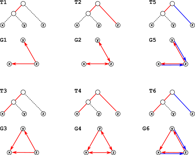
To establish the uniqueness of the least-resolved trees, we will consider so-called informative triples as shown in Fig. 4. Due to Lemma 3.2, it is an easy exercise to verify that each edge-labeled graph $G_{i}$, $i\in\{1,\dots,6\}$ in Fig. 4 is explained by the unique edge-labeled binary tree $T_{i}$, i.e., a specific labeled triple

Figure 4: Shown is the graph representation for six possible 3-vertex induced edge-labeled subgraphs $G_{1},\dots,G_{6}$ of a generalized Fitch graph$(K_{|X|},\varepsilon)$ that is explained by a tree $(T,\lambda)$. The $\otimes$-edges in each graph $G_{i}$ are omitted. Each subgraph $G_{1},\dots,G_{6}$ is explained by the unique edge-labeled triple $T_{1},\dots,T_{6}$, respectively. In each tree $T_{i}$, the $\otimes$-edges are drawn as dashed-lines and red-edges and blue-edges correspond to two distinct symbols $m,m^{\prime}\neq\otimes$. Edges in $T_{1},\dots,T_{6}$ can be understood as paths in $T$, whereby red-lined (resp. blue-lined, black-dashed) edges indicate that there is an $m$-edge (resp. $m^{\prime}$-edge, only $\otimes$-edges) on the particular path.

Definition 3.7.

An edge-labeled triple $ab|c$ is informative if it explains a 3-vertex induced subgraphs of a Fitch graph $(K_{|X|},\varepsilon)$ isomorphic to one of $G_{1},\dots G_{5}$ or $G_{6}$.

The observation that each graph $G_{i}$, $i\in\{1,\dots,6\}$ in Fig. 4 is explained by the unique edge-labeled binary tree $T_{i}$ is crucial, as this implies that whenever $(K_{|X|},\varepsilon)$ contains an induced subgraph of the form $G_{1},\dots G_{5}$ or $G_{6}$, then any tree explaining $(K_{|X|},\varepsilon)$ must display the corresponding informative triple. Any tree-like relation $\varepsilon$ can therefore be associated with a uniquely defined set ${R_{\varepsilon}}$ of informative triples that it displays: $r\in{R_{\varepsilon}}$ if and only if $r$ is the unique edge-labeled triple explaining an induced subgraph isomorphic to $G_{1},\dots G_{5}$ or $G_{6}$. For later reference we summarize this fact as

Lemma 3.8.

If $(T,\lambda)$ explains $\varepsilon$, then all triples in ${R_{\varepsilon}}$ must be displayed by $(T,\lambda)$.

In what follows, we want to show that ${R_{\varepsilon}}$ identifies the least-resolved tree that explains $\varepsilon$. To this end, we will utilize the following two results.

Lemma 3.9.

If $(T^{*},\lambda^{*})$ is a least-resolved tree for the tree-like map $\varepsilon:[X\times X]_{\textrm{irr}}\to M^{\otimes}$, then $(T^{*},\lambda^{*})$ contains no inner $\otimes$-edges and any inner vertex $v\neq\rho_{T^{*}}$ of $(T^{*},\lambda^{*})$ is incident to an outer $\otimes$-edge.

Proof.

First, assume for contradiction that the least-resolved tree $(T^{*},\lambda^{*})$ contains an inner $\otimes$-edge $e=uv$. The contraction of the edge $e$ does not change the number of $m$-edges with $m\neq\otimes$ along the paths connecting any two leaves. It affects the least common ancestor of $x$ and $y$, if $\operatorname{lca}_{T}(x,y)=u$ or $\operatorname{lca}_{T}(x,y)=v$. In either case, however, the number of $m$-edges between the $\operatorname{lca}_{T}(x,y)$ and the leaves $x$ and $y$ remains unchanged. Hence, the map $\varepsilon$ can still be explained by the tree that is obtained from $(T^{*},\lambda^{*})$ after contraction of $e$. Thus, $(T^{*},\lambda^{*})$ is not least-resolved; a contradiction.

We continue to show that any inner vertex $v$ must be incident to some outer $\otimes$-edge. Let $e=uv$ be the edge in $T^{*}$ with $u\succ_{T^{*}}v$. Let $F$ be the set of edges that are incident to $v$ and distinct from $e$. First assume, for contradiction, that all edges in $F$ have a label different from $\otimes$. If there are two edges $f,f^{\prime}\in F$ with distinct labels, then Lemma 3.2 implies that $e$ must be an $\otimes$-edge. However, $(T^{*},\lambda^{*})$ contains no inner $\otimes$-edges and, hence, all edges in $F$ must have the same label $m\neq\otimes$. In this case, Lemma 3.2 implies that the label $\lambda^{*}(e)$ of $e$ must be $m$ or $\otimes$. In either case, the edge $e$ can be contracted, since every path from $u$ to a leaf contains already an $m$-edge that is incident to $v$. Thus, $(T^{*},\lambda^{*})$ is not least-resolved; a contradiction. Therefore, $v$ must be incident to at least one $\otimes$-edge $f\in F$. Since $(T^{*},\lambda^{*})$ contains no inner $\otimes$-edges, the edge $f$ must be an outer-edge. ∎

Lemma 3.10.

Each inner edge in a least-resolved tree $(T^{*},\lambda^{*})$ for a tree-like map $\varepsilon:[X\times X]_{\textrm{irr}}\to M^{\otimes}$, is distinguished by at least one informative triple in ${R_{\varepsilon}}$.

Proof.

Consider an arbitrary inner edge $e=uv$ of $T^{*}$ with $u\succ_{T^{*}}v$. Since $(T^{*},\lambda^{*})$ is phylogenetic, there are necessarily leaves $x$, $y$, and $z$ such that $\operatorname{lca}(x,y)=v$ and $\operatorname{lca}(x,y,z)=u$. In particular, one can choose $y$ such that $vy$ is an outer $\otimes$-edge, since $(T^{*},\lambda^{*})$ is least-resolved and due to Lemma 3.9. Moreover, Lemma 3.9 implies that $\lambda^{*}(e)=m\neq\otimes$. Lemma 3.2 implies that all edges $f$ that are located in $T^{*}$ below $e$ must be $\otimes$- or $m$-edges. Thus, there are two exclusive cases for the path from $\operatorname{lca}(x,y)$ to $x$: Either the path contains (a) only $\otimes$-edges or (b) at least one $m$-edge. Moreover, the path $P_{u,z}$ from $u$ to $z$ contains either (A) only $\otimes$-edges or (B) an $m$-edge or (C) an $m^{\prime}$-edge with $m^{\prime}\neq m,\otimes$. Note, Lemma 3.2 implies that in case (A) (resp. (B)) all edges in $P_{u,z}$ must be $m$- or $\otimes$-edges (resp. $m^{\prime}$- or $\otimes$-edges). Now, the combination of the Cases (a) and (b) with (A), (B) or (C) immediately implies that the tree on $\{x,y,z\}$ displayed by $T^{*}$ must be one of the trees $T_{1},\dots,T_{5}$ or $T_{6}$ as shown in Fig. 4. Therefore, $xy|z\in{R_{\varepsilon}}$. Since $\operatorname{lca}(x,y)=v$ and $\operatorname{lca}(x,y,z)=u$, the edge $e$ is by definition distinguished by the triple $xy|z\in{R_{\varepsilon}}$. ∎

Theorem 3.11.

Let $\varepsilon:[X\times X]_{\textrm{irr}}\to M^{\otimes}$ be a tree-like map and $(T^{*},\lambda^{*})$ be a least-resolved tree that explains $\varepsilon$. Then, the set ${R_{\varepsilon}}$ identifies $(T^{*},\lambda^{*})$ and $\operatorname{Aho}({R_{\varepsilon}})=T^{*}$. In particular, $(T^{*},\lambda^{*})$ is unique up to isomorphism.

Proof.

We start with showing that ${R_{\varepsilon}}$ identifies $T^{*}$. If ${R_{\varepsilon}}=\emptyset$, then $(T^{*},\lambda^{*})$ must be a star tree, i.e., an edge-labeled tree that consists of outer edges only. Otherwise, $(T^{*},\lambda^{*})$ contains inner edges that are, by Lemma 3.10, distinguished by at least one informative rooted triple in ${R_{\varepsilon}}$, contradicting that ${R_{\varepsilon}}=\emptyset$. Hence, $r(T^{*})=\emptyset$, and therefore, $r(T^{*})=\operatorname{cl}({R_{\varepsilon}})$. Lemma 2.1 implies that ${R_{\varepsilon}}$ identifies $(T^{*},\lambda^{*})$.

In the case ${R_{\varepsilon}}\neq\emptyset$, assume for contradiction that $r(T^{*})\neq\operatorname{cl}({R_{\varepsilon}})$. By Lemma 3.8 we have ${R_{\varepsilon}}\subseteq r(T^{*})$. Isotony of the closure, Theorem 3.1(3) in [5], ensures $\operatorname{cl}({R_{\varepsilon}})\subseteq\operatorname{cl}(r(T^{*}))=r(T^{*})$. Our assumption therefore implies $\operatorname{cl}({R_{\varepsilon}})\subsetneq r(T^{*})$, and thus the existence of a triple $ab|c\in r(T^{*})\setminus\operatorname{cl}({R_{\varepsilon}})$. In particular, therefore, $ab|c\notin{R_{\varepsilon}}$. Note that neither $ac|b$ nor $bc|a$ can be contained in ${R_{\varepsilon}}$, since $(T^{*},\lambda^{*})$ explains $\varepsilon$ and, by assumption, already displays the triple $ab|c$. Thus, ${R_{\varepsilon}}$ contains no triples on $\{a,b,c\}$.

Let $u=\operatorname{lca}(a,b,c)$ and $e=uv$ be the edge in $T^{*}$ with $u\succ_{T^{*}}v\succeq_{T^{*}}\operatorname{lca}(a,b)$. By Lemma 3.9, the edge $e$ must be an $m$-edge with $m\neq\otimes$. Let $T_{abc}$ be the subtree of $(T,\lambda)$ with leaves $a,b,c$. Since $e$ is an $m$-edge, Lemma 3.2 implies that all edges along the paths from $v$ to $a$ and $v$ to $b$ must be $m$- or $\otimes$-edges. However, since $ab|c\notin{R_{\varepsilon}}$, the tree $T_{abc}$ cannot be isomorphic to the subtree $T_{1},\dots,T_{6}$ and thus, both paths from $\operatorname{lca}(a,b)$ to $a$ and $\operatorname{lca}(a,b)$ to $b$ must contain $m$-edges.

Moreover, Lemma 3.9 implies that there must be an outer $\otimes$-edge $f=vd$. By the discussion above, $d\neq a,b$. Thus, the the subtrees $T_{acd}$ and $T_{bcd}$ of $T^{*}$ with leaves $a,c,d$ and $b,c,d$, respectively, correspond to one the trees $T_{3},T_{4}$ and $T_{6}$. By construction, $ad|c\in{R_{\varepsilon}}$ and $bd|c\in{R_{\varepsilon}}$. Hence, any tree that explains $\varepsilon$ must display $ad|c$ and $bd|c$. As shown in [10], a tree displaying $ad|c$ and $bd|c$ also displays $ab|c$. This implies, however, that $ab|c\in\operatorname{cl}({R_{\varepsilon}})$, a contradiction to our assumption.

Therefore, $\operatorname{cl}({R_{\varepsilon}})=r(T)$ and we can apply Lemma 2.1 to conclude that ${R_{\varepsilon}}$ identifies $(T^{*},\lambda^{*})$ and $\operatorname{Aho}({R_{\varepsilon}})=T^{*}$.

We continue to show the uniqueness of $(T^{*},\lambda^{*})$. Since ${R_{\varepsilon}}$ identifies $(T^{*},\lambda^{*})$, any tree that displays ${R_{\varepsilon}}$ is by definition a refinement of $(T^{*},\lambda^{*})$. In addition, any tree that explains $\varepsilon$ must display ${R_{\varepsilon}}$ (cf. Lemma 3.8). Taken the latter two arguments together, any tree that explains $\varepsilon$ must be a refinement of $(T^{*},\lambda^{*})$.

To establish uniqueness of $(T^{*},\lambda^{*})$ it remains to show that there is no other labeling $\lambda$ such that $(T^{*},\lambda)$ still explains $\varepsilon$. Let $e=uv$ be an outer edge. Hence, changing the label of $e$ would immediately change the label $\varepsilon(w,v)$ between $v$ and any leaf $w$ located in a subtree rooted at a sibling of $v$. Since at least one such leaf $w$ exists in a phylogenetic tree, the edge $e$ cannot be re-labeled. Now suppose that $e=uv$ is an inner edge with $u\succ_{T^{*}}v$. By Lemma 3.9, the edge $e$ must be $m$-edge and $m\neq\otimes$. and there must be an outer $\otimes$-edge $f=vw$. Let $x$ be a leaf such that $\operatorname{lca}(w,x)=u$. Since $T^{*}$ is a phylogenetic tree, such a leaf always exists. Then $\varepsilon(x,w)=m$ if and only if $\lambda(e)=m$, i.e., the inner edge $e$ cannot be re-labeled. This establishes the final statement. ∎

4 Summary and Outlook

We have considered maps $\varepsilon:[X\times X]_{\textrm{irr}}\to M^{\otimes}$ and edge labeled di-graphs $(K_{|X|},\varepsilon)$ that can be explained by edge-labeled phylogenetic trees. Such graphs generalize the notion of xenology and simple Fitch graphs [20, 21]. As a main result, we gave a characterization of Fitch graphs based on four simple conditions (T1) to (T4) that are defined in terms of underlying edge-disjoint subgraphs. This in turn led to an $O(|X|^{2})$-time algorithm to recognize Fitch graphs $(K_{|X|},\varepsilon)$ and for the reconstruction of the unique least-resolved $M^{\otimes}$-edge-labeled phylogenetic tree that can explain them.

From the combinatorial point of view it might be of interest to consider more general maps $\mathcal{E}:[X\times X]_{\textrm{irr}}\to\mathcal{P}(M)\cup\{\otimes\}$, where $\mathcal{P}(M)$ denotes the powerset of $M$. In this case, there are a couple of ways to define when $\mathcal{E}$ is tree-like. The two most obvious ways, which we call “Type-1” and “Type-2” tree-like, are stated here.

The map $\mathcal{E}$ is tree-like

of Type-1,

if there is an edge-labeled tree $(T,\lambda)$ on $X$ such that for at least one $m\in\mathcal{E}(x,y)$ there is an edge on the path from $\operatorname{lca}(x,y)$ to $y$ with label $m$.

of Type-2,

if there is an edge-labeled tree $(T,\lambda)$ on $X$ such that for all $m\in\mathcal{E}(x,y)$ there is an edge on the path from $\operatorname{lca}(x,y)$ to $y$ with label $m$.

Note, if $|M|=1$ or $|\mathcal{E}(x,y)|=1$ for all $x,y\in X$, then the problem of determining whether $\mathcal{E}$ is Type-1 or Type-2 tree-like reduces to the problem of determining whether $(K_{|X|},\mathcal{E})$ is a Fitch graph or not. Moreover, if the sets $\mathcal{E}(x,y)$, $x,y\in X$ are pairwise disjoint, we can define a set $N=\{m_{\mathcal{E}(x,y)}\mid x,y\in X\}$ of symbols that identifies each symbol $m_{\mathcal{E}(x,y)}$ with the set $\mathcal{E}(x,y)$. The established results imply the following

Corollary 4.1.

If the map $\varepsilon:[X\times X]_{\textrm{irr}}\to N\cup\{\otimes\}$ with $\varepsilon(x,y)=m_{\mathcal{E}(x,y)}$ is tree-like, then the map $\mathcal{E}$ is tree-like of Type-1.

It would be of interest to understand such generalized tree-like maps in more detail. To this end, results established in [35, 2, 29] might shed some light on this question. Moreover, maps that cannot be explained by trees may be explained by phylogenetic networks, an issue that has not been addressed so-far.

References

- [1] Alfred V. Aho, Yehoshua Sagiv, Thomas G. Szymanski, and Jeffrey D. Ullman. Inferring a tree from lowest common ancestors with an application to the optimization of relational expressions. SIAM Journal on Computing, 10(3):405–421, 1981.
- [2] Hans-Jürgen Bandelt and Michael Anthony Steel. Symmetric matrices representable by weighted trees over a cancellative abelian monoid. SIAM Journal on Discrete Mathematics, 8(4):517–525, 1995.
- [3] S. Böcker and A. W. M. Dress. Recovering symbolically dated, rooted trees from symbolic ultrametrics. Adv. Math., 138:105–125, 1998.
- [4] J L Boore. The use of genome-level characters for phylogenetic reconstruction. Trends Ecol Evol, 21:439–446, 2006.
- [5] D. Bryant. Building trees, hunting for trees, and comparing trees: theory and methods in phylogenetic analysis. PhD thesis, University of Canterbury, 1997.
- [6] D. Bryant and M. Steel. Extension Operations on Sets of Leaf-Labeled Trees. Advances in Applied Mathematics, 16(4):425–453, December 1995.
- [7] D. G. Corneil, H. Lerchs, and L. Steward Burlingham. Complement reducible graphs. Discr. Appl. Math., 3:163–174, 1981.
- [8] C. Crespelle and C. Paul. Fully dynamic recognition algorithm and certificate for directed cographs. Discr. Appl. Math., 154:1722–1741, 2006.
- [9] Eric J. Deeds, Hooman Hennessey, and Eugene I. Shakhnovich. Prokaryotic phylogenies inferred from protein structural domains. Genome Res, 15:393–402, 2005.
- [10] M. C. H. Dekker. Reconstruction methods for derivation trees. Master’s thesis, Vrije Universiteit, Amsterdam, Netherlands, 1986.
- [11] Frédéric Delsuc, Henner Brinkmann, and Hervé Philippe. Phylogenomics and the reconstruction of the tree of life. Nature Reviews Genetics, 6(5):361–375, 2005.
- [12] Alexander Donath and Peter F. Stadler. Molecular morphology: Higher order characters derivable from sequence information. In J. Wolfgang Wägele and Thomas Bartolomaeus, editors, Deep Metazoan Phylogeny: The Backbone of the Tree of Life. New insights from analyses of molecules, morphology, and theory of data analysis, chapter 25, pages 549–562. de Gruyter, Berlin, 2014.
- [13] B. E. Dutilh, B. Snel, T. J. Ettema, and M. A. Huynen. Signature genes as a phylogenomic tool. Mol. Biol. Evol., 25:1659–1667, 2008.
- [14] A. Ehrenfeucht and G. Rozenberg. Theory of 2-structures, part I: Clans, basic subclasses, and morphisms. Theor. Comp. Sci., 70:277–303, 1990.
- [15] A. Ehrenfeucht and G. Rozenberg. Theory of 2-structures, part II: Representation through labeled tree families. Theor. Comp. Sci., 70:305–342, 1990.
- [16] J. Engelfriet, T. Harju, A. Proskurowski, and G. Rozenberg. Characterization and complexity of uniformly nonprimitive labeled 2-structures. Theor. Comp. Sci., 154:247–282, 1996.
- [17] W. M. Fitch. Homology a personal view on some of the problems. Trends Genet., 16:227–231, 2000.
- [18] Walter M. Fitch. Distinguishing Homologous from Analogous Proteins. Systematic Biology, 19(2):99–113, June 1970.
- [19] T. Gabaldón and EV. Koonin. Functional and evolutionary implications of gene orthology. Nat. Rev. Genet., 14(5):360–366, 2013.
- [20] M. Geiß, J. Anders, P.F. Stadler, N. Wieseke, and M. Hellmuth. Reconstructing gene trees from Fitch’s xenology relation. 2017. arXiv:1711.02152.
- [21] M. Geiß, M. Hellmuth, Y. Long, and P.F. Stadler. A short note on undirected fitch graphs. Art Discrete Appl. Math., 1(1):#P1.08, 2018.
- [22] S. Grünewald, Y. Long, and Y. Wu. Reconstructing unrooted phylogenetic trees from symbolic ternary metrics. Bulletin of Mathematical Biology, 2018. https://doi.org/10.1007/s11538-018-0413-7.
- [23] Stefan Grünewald, Mike Steel, and M. Shel Swenson. Closure operations in phylogenetics. Mathematical Biosciences, 208(2):521–537, August 2007.
- [24] M. Hellmuth, M. Hernandez-Rosales, K. T. Huber, V. Moulton, P. F. Stadler, and N. Wieseke. Orthology relations, symbolic ultrametrics, and cographs. J. Math. Biology, 66(1-2):399–420, 2013.
- [25] M. Hellmuth, M. Hernandez-Rosales, Y. Long, and P.F. Stadler. Inferring phylogenetic trees from the knowledge of rare evolutionary events. J. Math. Biology, 76(7):1623–1653, 2018.
- [26] M. Hellmuth, P.F. Stadler, and N. Wieseke. The mathematics of xenology: Di-cographs, symbolic ultrametrics, 2-structures and tree-representable systems of binary relations. J. Math. Biol., 75(1):199–237, 2017.
- [27] M. Hellmuth and N. Wieseke. From sequence data incl. orthologs, paralogs, and xenologs to gene and species trees. In Evolutionary Biology, pages 373–392, Cham, 2016. Springer International Publishing.
- [28] M. Hellmuth, N. Wieseke, M. Lechner, H.-P. Lenhof, M. Middendorf, and P.F. Stadler. Phylogenomics with paralogs. Proceedings of the National Academy of Sciences, 112(7):2058–2063, 2015. DOI: 10.1073/pnas.1412770112.
- [29] K.T. Huber, G. Scholz, and V. Moulton. Three-way symbolic tree-maps and ultrametrics. Journal of Classification, 2018. (in press).
- [30] Veiko Krauss, Christian Thümmler, Franziska Georgi, Jörg Lehmann, Peter F. Stadler, and Carina Eisenhardt. Near intron positions are reliable phylogenetic markers: An application to Holometabolous Insects. Mol. Biol. Evol., 25:821–830, 2008.
- [31] Sonja J. Prohaska, Claudia Fried, Chris T. Amemiya, Frank H. Ruddle, Günter P. Wagner, and Peter F. Stadler. The shark HoxN cluster is homologous to the human HoxD cluster. J. Mol. Evol., page 58, 2004. 212-217.
- [32] I B Rogozin, A V Sverdlov, V N Babenko, and E V Koonin. Analysis of evolution of exon-intron structure of eukaryotic genes. Brief Bioinform, 6:118–134, 2005.
- [33] A Rokas and P W Holland. Rare genomic changes as a tool for phylogenetics. Trends Ecol Evol, 15:454–459, 2000.
- [34] Carsten R. Seemann and Marc Hellmuth. The matroid structure of representative triple sets and triple-closure computation. European Journal of Combinatorics, 70:384 – 407, 2018.
- [35] Charles Semple and Mike Steel. Tree representations of non-symmetric group-valued proximities. Advances in Applied Mathematics, 23(3):300 – 321, 1999.
- [36] Charles Semple and Mike Steel. Phylogenetics, volume 24 of Oxford Lecture Series in Mathematics and its Applications. Oxford University Press, Oxford, 2003.
- [37] A M Shedlock and N Okada. SINE insertions: powerful tools for molecular systematics. BioEssays, 22:148–160, 2000.
- [38] Mike Steel. Phylogeny: Discrete and Random Processes in Evolution. CBMS-NSF Regional Conference Series in Applied Mathematics. Society for Industrial and Applied Mathematics, Philadelphia, November 2016.
- [39] R L Tatusov, M Y Galperin, D A Natale, and E V Koonin. The COG database: a tool for genome-scale analysis of protein functions and evolution. Nucleic Acids Research, 28(1):33–36, 2000.