Laplacian Dynamics on Cographs:
Controllability Analysis through Joins and Unions

Abstract

In this paper, we examine the controllability of Laplacian dynamic networks on cographs. Cographs appear in modeling a wide range of networks and include as special instances, the threshold graphs. In this work, we present necessary and sufficient conditions for the controllability of cographs, and provide an efficient method for selecting a minimal set of input nodes from which the network is controllable. In particular, we define a sibling partition in a cograph and show that the network is controllable if all nodes of any cell of this partition except one are chosen as control nodes. The key ingredient for such characterizations is the intricate connection between the modularity of cographs and their modal properties. Finally, we use these results to characterize the controllability conditions for certain subclasses of cographs.

I Introduction

Networks have become the backbone of the modern society. One foundational class of questions on networked systems pertains to their controllability [1, 2, 3, 4]. While there are classical tests to check the controllability of linear time-invariant (LTI) systems, their application to large-scale networks is numerically infeasible. Moreover, finding a minimum cardinality set of input nodes ensuring the controllability of a network is NP-hard. To overcome these issues, an alternative set of approaches involves adopting graph-theoretic techniques and connecting the controllability of a network to its topological features. In this direction, controllability analysis of networks with the so-called Laplacian dynamics has gained a lot of attention, partially due to their relevance in distributed algorithms as consensus, distributed estimation, and nonlinear synchronization [1, 5, 6, 7, 8]. In its most basic form, this dynamics is realized when the states of a network follow a consensus-type coordination protocol [9]. In such a dynamics, a subset of nodes in the network-known as leaders-are assumed to be controlled by external commands, while the other nodes-referred to as followers-follow the consensus (nearest-neighbor interaction) protocol. The controllability analysis of leader-follower Laplacian networks is of great interest in scenarios such as formation control, human-swarm interaction, and network security [10, 11].

There are two classes of results in the literature on the controllability analysis of Laplacian networks. In the first setting, necessary or sufficient conditions have been provided for network controllability. These conditions have been mainly stated in terms of notions such as graph symmetry [12, 13], equitable partitions [12, 14, 15, 5, 16, 17], distance partitions [15, 5], and pseudo monotonically increasing sequences [18, 7]. For example, the existence of a symmetry with respect to the leaders or control nodes of a network is known to be a sufficient condition for its uncontrollability [12]. There are, however, drawbacks to this line of work for analyzing large-scale networks. First, the known graph-theoretic conditions are not necessary and sufficient for network controllability; rather, these conditions are often used to obtain lower or/and upper bounds on the dimension of the controllable subspace. Furthermore, most of these results cannot be utilized for efficiently selecting input nodes ensuring the controllability of the network. For instance, finding a minimum cardinality set of nodes breaking symmetries for general networks is NP-hard [13]. We also mention the results reported in [8], where by identifying the structure of controllability destructive nodes, necessary and sufficient controllability conditions for Laplacian networks of size five or less have been established.

In order to derive stronger and readily applicable network-centric controllability conditions, in the second class of results, Laplacian networks with special graph topologies have been considered. In this case, controllability of networks with embedded path graphs [19, 20], cycle graphs [19], [21], complete graphs [15], circulant graphs [22], multi-chain graphs [23], grid graphs [24], and tree graphs [25] have been investigated. These approaches rely on the pattern of the Laplacian eigenvectors in conjunction with the Popov-Belevitch-Hautus (PBH) test to facilitate the controllability analysis. Moreover, a complete characterization of the eigenspaces of these graphs leads to efficient procedures for selecting the minimum number of control nodes from which the network is controllable. By considering the different methods of combining or growing controllable networks, this class of results can be also applied when designing network structures with desired controllability properties [26, 27]. However, the class of Laplacian networks with efficient graph-theoretic controllability conditions is still limited. In this paper, we further expand the applicability of such graph-theoretic conditions by examining the controllability of Laplacian networks defined over cographs.

Cographs have been independently rediscovered and reintroduced by different authors; as such, they assume multiple equivalent definitions. For example, in such graphs, there is no induced subgraph isomorphic to a path of size four, and accordingly they are called $P_{4}$-free graphs [28]. Moreover, some authors refer to cographs as decomposable graphs [29], or complement-reducible graphs [28], due to the fact that they can be generated through recursive operations of joins and unions starting from isolated nodes [30]. The sequence of these operations leads to a unique rooted tree representation of a cograph, referred to as a cotree [28]. Cographs arise in disperate areas of computer science and mathematics and find applications in areas such as scheduling [31, 32] and orthology detection [33]. In fact, thanks to their structural properties, many algorithmic problems that are NP-hard for general networks can be solved in a polynomial time over cographs [34]. Cographs have a close relationship with series-parallel networks that are used to model biological and electrical systems [35, 28]. Furthermore, there has been interest in identifying cograph communities and functional modules in social and biological networks in order to better reveal their local and global structures and functions [36, 37]. Cographs include other known classes of graphs, including complete graphs, complete bipartite graphs, cluster graphs, Turan graphs, and trivially-perfect graphs. In particular, threshold graphs are an important subclass of cographs with numerous applications in modeling social and psychological networks and synchronizing parallel processes [38, 39]. In the meantime, a connected threshold graph has certain limitations in modeling networked control systems; for example, it has at least one dominating node (that is adjacent to all other nodes), while a general cograph might not have such a node.

In [40], the controllability of threshold graphs from a single control node has been explored. Subsequently, in [41], the results of [40] have been extended to multi-input networks; however, the results provided in [41] are restrictive in the sense that it examines threshold graphs with only one repeated degree. In [42], the controllability problem of a general threshold graph has been solved for the case in which any input signal is assumed to be injected into only one node. Furthermore, in [43], the results of [42] have been extended to the case where the input matrix has binary entries. However, we note that unlike a general cograph, in a threshold graph, information about the set of eigenvalues and eigenvectors can be inferred from the sequence of node degrees. As such, the results of [42] and [43] cannot readily be applied in a more general setting, namely for networks that are characterized by cographs. In fact, the analysis approach adopted in the aforementioned works–relying on the creation sequence and node degrees of a threshold graph–does not apply for a general cograph. In this paper, we take a step towards studying the controllability problem for Laplacian networks defined on cographs.

Our first contribution is providing the spectrum and an associated modal matrix for a cograph. This is accomplished by considering the cotree representation of cographs, and subsequently showing that the set of nontrivial eigenvalues (respectively, eigenvectors) of a cograph is an updated version of the nontrivial eigenvalues (respectively, eigenvectors) generated at each internal node of the associated cotree. In this direction, we also illustrate some properties of eigenvalues of a cograph and their eigenspaces, using the structural feature of the associated cotree; this is discussed in §III. As the second and main contribution of this work, we establish necessary and sufficient conditions for controllability of Laplacian networks on cographs in §IV. In this direction, based on the fact that the uncontrollability of a network results from the zero entries of its eigenvectors, we identify all (and the only) nodes rendering a cograph controllable. In fact, we decompose a cograph into structurally equivalent subgroups or cells, essentially playing similar roles in the network dynamics. By defining a sibling partition in a cograph, we then demonstrate that these cells include sibling nodes that interact similarly with all other nodes in the graph. Thus, in order to break “structural symmetries” in a cograph, all nodes of any cell except one should be directly controlled. Particularly, it is proven that the minimum number of control nodes to completely control a cograph is the difference between its size and the number of cells of its sibling partition. Finally, we provide an alternate approach for obtaining the results reported in [42, 43], when the controllability conditions for general cographs are interpreted in the context of its subclasses, such as the threshold graphs.

II Preliminaries

In this section, necessary preliminaries for our subsequent discussion are reviewed.
Notation: The set of real numbers is denoted by $\mathbb{R}$. For a set $\mathcal{S}$, its cardinality is denoted by $|\mathcal{S}|$. For a matrix $M\in\mathbb{R}^{p\times q}$ and a set of indices $\mathcal{S}$, $M_{\mathcal{S},:}\in\mathcal{R}^{|\mathcal{S}|\times q}$ is a submatrix of $M$ whose rows are the indices from $\mathcal{S}$. The $n\times n$ identity matrix is denoted by $I_{n}$, and $e_{j}$ represents its $j$th column. The vectors of all 1’s and all 0’s with size $n$ are respectively denoted by $\textbf{1}_{n}$ and $\textbf{0}_{n}$. The $n\times m$ matrix of all 1’s (respectively, all 0’s) is designated as $\textbf{1}_{n\times m}$ (respectively, $\textbf{0}_{n\times m}$). For notational convenience, for a vector $v\in\mathbb{R}^{n}$ and a scalar $m\in\mathbb{R}$, we write $v+m$ to represent $v+m\textbf{1}_{n}$.

Graph: A directed graph $G$ of size $n$ is represented by $G=(V,E)$, where $V=\{1,\ldots,n\}$ is its node set, and $E\subset V\times V$ denotes its edge set. We say $(i,j)\in E$ if there is a directed edge from the node $i$ to the node $j$. A directed path from the node $i_{1}\in V$ to the node $i_{k}\in V$ is a sequence of distinct nodes $(i_{1},i_{2},\ldots,i_{k})$, where for every $1\leq j\leq k-1$, $(i_{j},i_{j+1})\in E$. The graph $G$ is undirected if for every edge $(i,j)\in E$, we have $(j,i)\in E$; in this case, we write $\{i,j\}\in E$, and we refer to node $j$ (respectively, $i$) as the neighbor of the node $i$ (respectively, $j$). For an undirected graph $G$, we denote by $N(i)$ the set of neighbors of $i\in V$. The degree of the node $i$ is defined as $d(i)=|N(i)|$. The degree matrix of an undirected graph $G$ is defined as $\Delta(G)=\mathrm{diag}(d(1),\ldots,d(n))$. The corresponding Laplacian matrix $L(G)$ is given by $L(G)=\Delta(G)-A(G)$, where $A(G)$ is the (0,1)-adjacency matrix associated with $G$. A complete graph $G=(V,E)$ is an undirected graph such that for all $i,j\in V$, $i\neq j$, $\{i,j\}\in E$; it is denoted by $K_{n}$. Consider two disjoint sets $V_{1}$ and $V_{2}$ of respectively size $n_{1}$ and $n_{2}$ such that $V=V_{1}\cup V_{2}$. A complete bipartite graph $G=(V,E)$, denoted by $K_{n_{1},n_{2}}$, is an undirected graph such that for any pair of nodes $i,j\in V_{k}$, $k=1,2$, $\{i,j\}\notin E$, while for any $i\in V_{1}$ and $j\in V_{2}$, $\{i,j\}\in E$. A path graph of size $n$, denoted by $P_{n}$, is a graph whose nodes can be indexed by $1,2,\ldots,n$ in such a way that for all $1\leq i\leq n-1$, $\{i,j\}\in E$ if and only if $j=i+1$. If two nodes of degree one in $P_{n}$ are connected, a cycle graph $C_{n}$ is obtained.

Rooted trees: Consider an undirected tree graph, and assign a direction to any of its edges. The new directed graph is a rooted tree and denoted by $\mathcal{T}=(V^{\mathcal{T}},E^{\mathcal{T}})$ if for a special node $r\in V^{\mathcal{T}}$, called the root, there is a unique directed path from $r$ to every node of $\mathcal{T}$. For a node $i\in V^{\mathcal{T}}$, a node $j\in V^{\mathcal{T}}$ such that $(i,j)\in E^{\mathcal{T}}$ (respectively, $(j,i)\in E^{\mathcal{T}}$) is called a child (respectively, parent) of $i$. A node $j\in V^{\mathcal{T}}$ is called a descendant (respectively, ancestor) of node $i\in V^{\mathcal{T}}$ if there is a directed path from $i$ to $j$ (respectively, from $j$ to $i$). The lowest common ancestor of two nodes $k,l\in V^{\mathcal{T}}$ is the shared ancestor of $k$ and $l$, which is located farthest from the root $r$ of $\mathcal{T}$. A node $i$ is called a leaf if it has no child; otherwise, it is an internal node of $\mathcal{T}$. The set of children of an internal node $v$ is given by ${\mathcal{C}}(v)$, and its size is denoted by $c(v)$. Moreover, the set of leaves descending from the internal node $v$ is represented by $\mathcal{L}(v)$; we define $l(v)=|\mathcal{L}(v)|$. The unique path from a node $w$ to its descendant $v$ is given by $\mathcal{P}_{v}^{w}$. A group of leaves with the same parent in the rooted tree $\mathcal{T}$ is referred to as siblings.

Example: In the rooted tree depicted in Fig. 1 (b), any node $i$, $1\leq i\leq 8$, is a leaf; while each node $v^{j}$, $1\leq j\leq 5$, is an internal node. Node $v^{3}$ is the root, and we have $\mathcal{C}(v^{3})=\{4,v^{2},v^{4}\}$. Thus, $c(v^{3})=3$. Also, one has $\mathcal{L}(v^{4})=\{5,6,7,8\}$, and $l(v^{4})=4$. Leaves 6, 7, and 8 have the same parent $v^{5}$, and thus are siblings. The path $\mathcal{P}_{v^{1}}^{v^{3}}$ can be described by the sequence $(v^{3},v^{2},v^{1})$. The lowest common ancestor of leaves 5 and 8 is $v^{4}$.

Eigenpairs: Consider an undirected graph $G=(V,E)$. For notational convenience, by eigenvalues and eigenvectors of $G$, we mean the eigenvalues and eigenvectors of its Laplacian matrix $L(G)$. Since $L(G)$ (for an undirected graph $G$) is symmetric and nonnegative, all of its eigenvalues are real and nonnegative [44]. Moreover, its smallest eigenvalue is zero with the associated eigenvector $\textbf{1}_{n}$. The vector $(0,\textbf{1}_{n})$ is known as a trivial eigenpair for any undirected graph $G$. Now, let $\Lambda(G)=(\lambda_{2},\ldots,\lambda_{n})$ be the nontrivial spectrum of $G$ including its nontrivial eigenvalues, and note that if $G$ is connected, $0\notin{\Lambda}(G)$. Next, let $\nu_{i}\in\mathbb{R}^{n}$ be a nonzero eigenvector of $G$ associated with $\lambda_{i}$, where $L(G)\nu_{i}=\lambda_{i}\nu_{i}$. Then, we define ${\mathcal{V}}(G)=[\nu_{2},\ldots,\nu_{n}]$ as a full rank nontrivial modal matrix of $G$ associated with ${\Lambda}(G)$. Let $\tilde{\lambda}_{1}$, $\ldots$, $\tilde{\lambda}_{r}$ be the $r$ distinct eigenvalues in ${\Lambda}(G)$. We can rewrite the nontrivial spectrum of a connected $G$ as ${\Lambda}(G)=(\tilde{\lambda}_{1}^{(q_{1})},\ldots,\tilde{\lambda}_{r}^{(q_{r})})$, where $q_{i}$ is the algebraic multiplicity of the nonzero eigenvalue $\tilde{\lambda}_{i}$. Since $L(G)$ is symmetric, for an eigenvalue $\tilde{\lambda}_{i}$ with the multiplicity $q_{i}$, there are $q_{i}$ independent eigenvectors spanning the eigenspace associated with $\tilde{\lambda}_{i}$. Let $\mathcal{V}^{(i)}\in\mathbb{R}^{n\times q_{i}}$ be a full rank matrix where $L(G)\mathcal{V}^{(i)}=\tilde{\lambda}_{i}\mathcal{V}^{(i)}$, $i=1,\ldots,r$. Then, the nontrivial modal matrix associated with ${\Lambda}(G)$ for a connected $G$ can be written as ${\mathcal{V}}(G)=[\mathcal{V}^{(1)},\ldots,\mathcal{V}^{(r)}]$.

II-A Cographs

In this part, cographs and related concepts are reviewed.

Let $G_{1}=(V_{1},E_{1})$ and $G_{2}=(V_{2},E_{2})$ be two disjoint undirected graphs of respectively, size $n_{1}$ and $n_{2}$. A graph $G=(V,E)$ is the union of $G_{1}$ and $G_{2}$ if $V=V_{1}\cup V_{2}$, and $E=E_{1}\cup E_{2}$; such a graph $G$ is written as $G=G_{1}+G_{2}$. A graph $G=(V,E)$ is the join of $G_{1}$ and $G_{2}$ if $V=V_{1}\cup V_{2}$, and $E=E_{1}\cup E_{2}\cup\{\{i,j\}:i\in V_{1}\>\mbox{and}\>j\in V_{2}\}$; thus $G$ is represented by $G=G_{1}*G_{2}$. Join and union operations obey the commutative and transitive properties. For example, we have $G_{1}+G_{2}=G_{2}+G_{1}$, and $G_{1}*(G_{2}*G_{3})=(G_{1}*G_{2})*G_{3}$. However, they are not distributive.

A graph is called a cograph (or a decomposable graph) if it can be constructed from isolated nodes by recursively performing join and union operations. More formally, a graph with a single node (i.e., $K_{1}$) is a cograph, and if $G_{1},\ldots,G_{k}$, for some $k>1$, are cographs, then $G_{1}+\ldots+G_{k}$ and $G_{1}*\ldots*G_{k}$ are cographs as well. Also, based on an equivalent definition, a graph is a cograph if it has no induced subgraphs isomorphic to $P_{4}$ [45]. Thus, for example, the cycle graph $C_{5}$ is not a cograph, while the complete graph $K_{4}$ is.

A cotree $\mathcal{T}=(V^{\mathcal{T}},E^{\mathcal{T}})$ associated with a connected cograph $G=(V,E)$ is a rooted tree whose leaves correspond to the nodes of the cograph. We index the leaves of a cotree by $i$, where $1\leq i\leq n$; while the internal nodes are represented here by $v^{j}$, for $1\leq j\leq h$. The root of the cotree $r$ is labeled as 1, and its internal nodes are labeled 0 or 1. For an internal node $v^{k}$, $\mathrm{lab}(v^{k})$ provides the label of $v^{k}$. Let $\mathcal{T}_{(z)}$ be a subtree of $\mathcal{T}$ which is rooted at some node $z\in V^{\mathcal{T}}$. Then, $\mathcal{T}_{(z)}$ corresponds to an induced subgraph of $G$ defined on the leaves which are descendants of $z$. We denote this subgraph by $G_{(z)}$, and call it a cograph associated with $z$. If $z$ is a leaf of $\mathcal{T}$, $G_{(z)}=(\{z\},\emptyset)$. In addition, if $z$ is an internal node that is labeled as 0 (respectively, 1), $G_{(z)}$ is the union (respectively, join) of the cographs associated with the children of $z$ [28].

Any cograph $G$ can be represented by a cotree $\mathcal{T}$, and if for any leaf $v$ of $\mathcal{T}$, the labels on the internal nodes of the path $\mathcal{P}_{v}^{r}$ alternate between 0 and 1, this representation is unique. A cograph $G=(V,E)$ can be recognized in $\mathcal{O}(|V|+|E|)$, while its associated cotree can be built in the same time-complexity [32]. Alternatively, one can form a cograph $G$ from a given cotree $\mathcal{T}$. In this direction, two nodes $i,j\in V$ are neighbors in $G$ if and only if the lowest common ancestor of the leaves $i,j\in V^{\mathcal{T}}$ is labeled 1.

In a cograph $G=(V,E)$, two nodes $i,j\in V$ are called siblings if the leaves $i$ and $j$ in the corresponding cotree are siblings. By this definition, it is known that $i,j\in V$ are siblings if $N(i)\setminus\{j\}=N(j)\setminus\{i\}$ [28].

Example: In Fig. 1, a cograph along with its associated cotree are illustrated. The cograph $G$ can be constructed through successive joins and unions as $G=[(K_{1}*K_{1})+K_{1}]*K_{1}*[K_{1}+(K_{1}*K_{1}*K_{1})]$. One can see that nodes 1, 2 and nodes 6, 7, 8 are siblings in this cograph. We have $\mathrm{lab}(v^{1})=1$, and $\mathrm{lab}(v^{4})=0$. The graph $G_{(v^{2})}$ is an induced subgraph of $G$ defined on nodes $1,2,3$. Since $\mathrm{lab}(v^{2})=0$, $G_{(v^{2})}$ is a union of $G_{(v^{1})}$ and $G_{(3)}$. The lowest common ancestor of nodes 5 and 8 is $v^{4}$, that is labeled 0; thus, these two nodes are not neighbors in $G$.

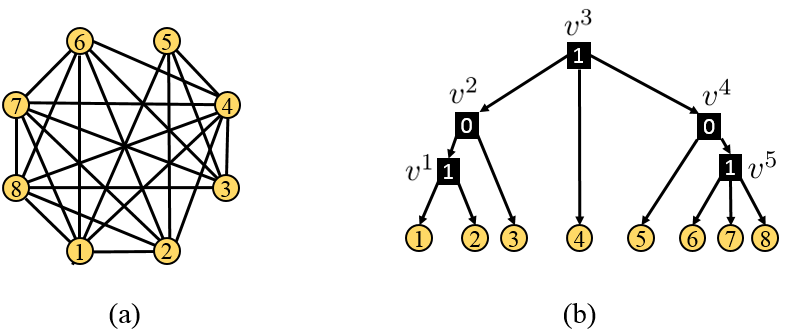
Figure 1: a) Cograph $G$, b) Associated cotree $\mathcal{T}$.

II-B Threshold Graphs

By starting from a single node, a threshold graph that is a special subclass of cographs is constructed by repeatedly adding a single node to the old graph through the join or the union operation. In other words, $K_{1}$ is a threshold graph; and if $G^{\prime}$ is a threshold graph, $G^{\prime}+K_{1}$ and $G^{\prime}*K_{1}$ are threshold graphs as well.

Example: In Fig. 2, a threshold graph $G$ and its corresponding cotree $\mathcal{T}$ are shown.

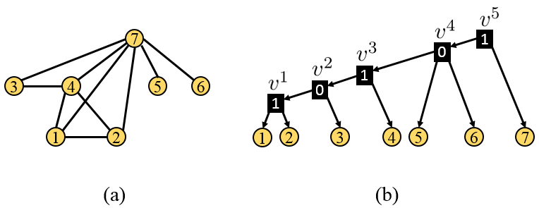
Figure 2: a) Threshold graph $G$, b) Associated cotree $\mathcal{T}$.

II-C Graph Symmetry

The symmetries in a graph can be described by its automorphism group [12, 5, 17]. Let $\sigma:V\rightarrow V$ be a permutation of the nodes of a graph $G=(V,E)$, where $\{u,v\}\in E$ if and only if $\{\sigma(u),\sigma(v)\}\in E$. Then such a $\sigma$ is referred to as an automorphism of $G$. A trivial automorphism of $G$ is a permutation fixing all nodes.

II-D Problem Formulation

In this paper, we consider a linear time-invariant (LTI) system defined on a connected cograph $G=(V,E)$ with the Laplacian dynamics described as,

$$\dot{x}=Ax+Bu,$$ (1)

where $A=-L(G)$, and $L(G)\in\mathbb{R}^{n\times n}$ is the Laplacian matrix associated with $G$. Moreover, $x=[x_{1},\ldots,x_{n}]^{T}$ is the aggregated vector of states of the nodes, and $u=[u_{1},\ldots,u_{m}]^{T}$ is the vector of inputs. Also, $B\in\mathbb{R}^{n\times m}$ is the input matrix whose nonzero entries determine the nodes where the input signals are directly injected. Here, we assume that any input signal can be injected into only one node, referred to as a control node. Thus, $B$ assumes the form,

$$B=[e_{j_{1}},\ldots,e_{j_{m}}],$$ (2)

where $j_{i}\in\{1,\ldots,n\}$, for $1\leq i\leq m$. We refer to $V_{C}=\{j_{1},\ldots,j_{m}\}$ as the set of control nodes.

The controllability of an LTI system captures the ability of an input to steer the states of the system from an arbitrary initial value to any final value within a finite time. In this paper, we aim to provide graph-theoretic controllability conditions for the network described in (1) and find the minimum number of control nodes from which the network is controllable. The celebrated Popov-Belevitch-Hautus (PBH) test has proved to be instrumental in bridging controllability analysis for networks to graph-theoretic constructs.

Proposition 1 ([46])

A system with dynamics (1) (or the pair $(A,B)$) is controllable if and only if for any (left) eigenvector $\nu$ of $A$, we have $\nu^{T}B\neq 0$.

Note that if we would like to select a set of control nodes for a network of size $n$ based on the PBH test, we can perform a brute-force verification of the required controllability condition for exponentially many combinations, a computationally impractical endeavor for large-scale networks. Thereby, in this paper, we aim to characterize controllability conditions that can be efficiently inferred from the network topology, specifically for cographs. The key ingredient for such characterizations is the intricate connection between the modularity of cographs and their modal properties.

The following proposition is one of the pertinent results, providing a necessary condition for controllability of a general network based on the existing symmetries in its structure.

Proposition 2 ([12, 13])

A network with dynamics (1) defined on a graph $G$ is uncontrollable if $G$ has a nontrivial automorphism that fixes the control nodes.

III Cographs Eigenvalues and Eigenvectors

In this section, we investigate the spectrum and an associated modal matrix of a cograph $G$. Indeed, in order to use the PBH test for controllability analysis of a cograph, we first characterize the eigenspace associated with any eigenvalue of $G$. Then, we find some conditions on the multiplicity of any eigenvalue, which denotes the dimension of the corresponding eigenspace. These results turn out to be instrumental to provide the controllability conditions for a cograph.

III-A Computing Eigenvalues and Eigenvectors of a Cograph

In this part, we compute the eigenvalues and linearly independent eigenvectors of a cograph. Indeed, to any internal node $v$ of a cotree, we associate a set of eigenvectors and an eigenvalue whose multiplicity is one less than the number of children of $v$. The next result is an extension of Theorem 2.1 of [29].

First, let $\Lambda_{i}=\Lambda(G_{i})$ and $\mathcal{V}_{i}=\mathcal{V}(G_{i})$ be respectively, the nontrivial spectrum and the associated nontrivial modal matrix of the graph $G_{i}$, $i=1,\ldots,p$ (note that for a graph $G_{i}$ of size one, $\Lambda(G_{i})=\emptyset$ and $\mathcal{V}(G_{i})=\emptyset$ ). Moreover, assume that the nodes of $G_{i}$ are indexed prior to nodes of $G_{j}$, for $1\leq i<j\leq p$.

Theorem 3

Consider the graphs $G_{1},G_{2},\ldots,G_{p}$ of respectively, size $n_{1},n_{2},\ldots,n_{p}$, and let $n=\sum_{i=1}^{p}n_{i}$. Then,

• $\Lambda(G_{1}+G_{2}+\ldots+G_{p})=(\Lambda_{1},\Lambda_{2},\ldots,\Lambda_{p},0^{(p-1)})$,
  

• $\Lambda(G_{1}*G_{2}*\ldots*G_{p})=\\ (\Lambda_{1}+n-n_{1},\Lambda_{2}+n-n_{2},\ldots,\Lambda_{p}+n-n_{p},n^{(p-1)})$,
  

• $\mathcal{V}(G_{1}+G_{2}+\ldots+G_{p})=\mathcal{V}(G_{1}*G_{2}*\ldots*G_{p})=\\ \begin{bmatrix}\mathcal{V}_{1}&\textbf{0}_{n_{1}}&\ldots&\textbf{0}_{n_{1}}&n_{2}\textbf{1}_{n_{1}}&\ldots&n_{p}\textbf{1}_{n_{1}}\\ \textbf{0}_{n_{2}}&\mathcal{V}_{2}&\ldots&\textbf{0}_{n_{2}}&-n_{1}\textbf{1}_{n_{2}}&\ldots&n_{p}\textbf{1}_{n_{2}}\\ \vdots&\vdots&\ddots&\vdots&\vdots&\ddots&\vdots\\ \textbf{0}_{n_{p}}&\textbf{0}_{n_{p}}&\ldots&\mathcal{V}_{p}&\textbf{0}_{n_{p}}&\ldots&-(\sum_{i=1}^{p-1}n_{i})\textbf{1}_{n_{p}}\end{bmatrix}$.

Proof: The proof is based on an inductive argument. For two graphs $G_{1}$ and $G_{2}$, one has ${\Lambda}(G_{1}+G_{2})=(\Lambda_{1},\Lambda_{2},0)$ and ${\Lambda}(G_{1}*G_{2})=(\Lambda_{1},\Lambda_{2},n_{1}+n_{2})$ [29]. Moreover,

$$\mathcal{V}(G_{1}+G_{2})=\mathcal{V}(G_{1}*G_{2})=\begin{bmatrix}\mathcal{V}_{1}&\textbf{0}_{n_{1}}&n_{2}\textbf{1}_{n_{1}}\\ \textbf{0}_{n_{2}}&\mathcal{V}_{2}&-n_{1}\textbf{1}_{n_{2}}\end{bmatrix}.$$ (3)

Thus the statement of the theorem holds for $p=2$. Now, assume that for $p=k$, the statement of the theorem is valid. We want to prove the claim for $p=k+1$. Consider $G_{1}+G_{2}+\ldots+G_{k}+G_{k+1}$ (respectively, $G_{1}*G_{2}*\ldots*G_{k}*G_{k+1}$) as $G^{\prime}+G_{k+1}$ (respectively, $G^{\prime}*G_{k+1}$), where $G^{\prime}=G_{1}+G_{2}+\ldots+G_{k}$ (respectively, $G^{\prime}=G_{1}*G_{2}*\ldots*G_{k}$). Thereby, using (3), the statement of the theorem is valid for $p=k+1$. $\blacksquare$

Before characterizing the nontrivial spectrum and an associated nontrivial modal matrix of a cograph, let us introduce more notation. For an internal node $v$ in a cotree $\mathcal{T}=(V^{\mathcal{T}},E^{\mathcal{T}})$, we recall that $\mathcal{C}(v)$ with $c(v)=|\mathcal{C}(v)|$, and $\mathcal{L}(v)$ with $l(v)=|\mathcal{L}(v)|$ are respectively, the set of children and leaves descending from $v$. Let $c(v)=k$, and $\mathcal{C}(v)=\{v_{1},\ldots,v_{k}\}$. Note that $k>1$. Now, define $\lambda_{\mathrm{new}}(v)=\mathrm{lab}(v)\times l(v)$, which is referred to as the new eigenvalue of the internal node $v$. Then, if $\mathrm{lab}(v)=0$, $\lambda_{\mathrm{new}}(v)=0$, and if $\mathrm{lab}(v)=1$, $\lambda_{\mathrm{new}}(v)=l(v)$. Now, let $n_{i}=l(v_{i})$, $1\leq i\leq k$, and consider the matrix $M\in\mathbb{R}^{l(v)\times(k-1)}$ as

$$\scriptsize M=\begin{bmatrix}n_{2}\textbf{1}_{n_{1}}&\ldots&n_{k-1}\textbf{1}_{n_{1}}&n_{k}\textbf{1}_{n_{1}}\\ -n_{1}\textbf{1}_{n_{2}}&\ldots&n_{k-1}\textbf{1}_{n_{2}}&n_{k}\textbf{1}_{n_{2}}\\ \vdots&\ddots&\vdots&\vdots\\ \textbf{0}_{n_{k-1}}&\ldots&-\sum_{j=1}^{k-2}n_{j}\textbf{1}_{n_{k-1}}&n_{k}\textbf{1}_{n_{k-1}}\\ \textbf{0}_{n_{k}}&\ldots&\textbf{0}_{n_{k}}&-\sum_{j=1}^{k-1}n_{j}\textbf{1}_{n_{k}}\\ \end{bmatrix}.$$

Let us define $\mathcal{V}_{\mathrm{new}}(v)=M$, which we refer to as a new modal matrix of the internal node $v$.

Now, consider two internal nodes $v,w\in V^{\mathcal{T}}$, where $w$ is an ancestor of $v$. Let $\mathcal{P}_{v}^{w}=(u_{0},u_{1},\ldots,u_{p})$, where $u_{0}=w$ and $u_{p}=v$. Then, for an eigenvalue $\lambda\in\Lambda(G_{(v)})$, if $v=w$, the updated eigenvalue of $v$ at $w$ is defined as $\lambda_{\mathrm{upd}}^{w}(v)=\lambda_{\mathrm{new}}(v)$; otherwise, it is defined as

$$\lambda_{\mathrm{upd}}^{w}(v)=\lambda_{\mathrm{new}}(v)+\sum_{i=0}^{p-1}\mathrm{lab}(u_{i})\times(l(u_{i})-l(u_{i+1})).$$

In addition, let $\mathcal{V}^{\prime}\in\mathbb{R}^{l(w)\times(c(v)-1)}$ be such that $\mathcal{V}^{\prime}_{\mathcal{L}(v),:}=\mathcal{V}_{\mathrm{new}}(v)$, and $\mathcal{V}^{\prime}_{\mathcal{L}(w)\setminus\mathcal{L}(v),:}=\textbf{0}_{(l(w)-l(v))\times(c(v)-1)}$. In other words, $\mathcal{V}^{\prime}$ is a $l(w)\times(c(v)-1)$ matrix whose rows corresponding to the indices of leaves of $G_{(v)}$ constitute the matrix $\mathcal{V}_{\mathrm{new}}(v)$, while the rest of its rows are the zero vectors. Let us define the updated modal matrix of $v$ at $w$ as $\mathcal{V}_{\mathrm{upd}}^{w}(v)=\mathcal{V}^{\prime}$. It is obvious that $\mathcal{V}_{\mathrm{upd}}^{v}(v)=\mathcal{V}_{\mathrm{new}}(v)$.

Theorem 4

Consider a cograph $G=(V,E)$ with the associated cotree $\mathcal{T}=(V^{\mathcal{T}},E^{\mathcal{T}})$ and the root $r$. Let $h=|V^{\mathcal{T}}|-|V|$ be the number of internal nodes of $\mathcal{T}$, and let $v^{1},\ldots,v^{h}$ be its internal nodes. For $1\leq i\leq h$, let $\lambda_{i}=\lambda_{\mathrm{upd}}^{r}(v^{i})$, and $\mathcal{V}^{(i)}=\mathcal{V}_{\mathrm{upd}}^{r}(v^{i})$. Then,

$$\Lambda(G)=(\lambda_{1}^{(c(v^{1})-1)},\ldots,\lambda_{h}^{(c(v^{h})-1)}),$$ (4)

$$\mathcal{V}(G)=[\mathcal{V}^{(1)},\ldots,\mathcal{V}^{(h)}].$$ (5)

Proof: The proof follows by a strong induction on $h$. First, we show that the result holds for $h=1$. Let $v$ be the single internal node with $c(v)=l(v)=n$, and note that $r=v$. Then, the children of $v$ are all graphs of size one. Thus, from Theorem 3, if $\mathrm{lab}(v)=0$, $\Lambda(G)=(0^{(n-1)})$, and otherwise $\Lambda(G)=(n^{(n-1)})$. Hence, $\lambda_{\mathrm{upd}}^{r}(v)=\lambda_{\mathrm{new}}^{r}(v)=\mathrm{lab}(v)\times l(v)$, and for $\lambda=\lambda_{\mathrm{upd}}^{r}(v)$, one can write $\Lambda(G)=(\lambda^{(c(v)-1)})$. Moreover, Theorem 3 implies that

$$\scriptsize\mathcal{V}(G)=\begin{bmatrix}1&\ldots&1&1\\ -1&\ldots&1&1\\ \vdots&\ddots&-(n-2)&1\\ 0&\ldots&0&-(n-1)\end{bmatrix}$$ (6)

Consequently, one can write $\mathcal{V}(G)=\mathcal{V}_{\mathrm{upd}}^{r}(v)$; the result is thus valid for $h=1$. Now, assuming that the result holds for all $h\leq k$, we want to prove that it holds for $h=k+1$. Let $r=v^{k+1}$, and $c(r)=p$. Further, let $\mathcal{C}(r)=\{u_{1},\ldots,u_{p}\}$. Let us index the leaves of $\mathcal{T}$ in a way that for $1\leq i<j\leq p$, leaves of $\mathcal{T}_{(u_{i})}$ are indexed prior to the leaves of $\mathcal{T}_{(u_{j})}$. Since the number of internal nodes of every $\mathcal{T}_{(u_{i})}$, $1\leq i\leq p$, is less than $k+1$, by our inductive hypothesis, we know that $\Lambda(G_{(u_{i})})$ is a sequence of $\lambda_{\mathrm{upd}}^{u_{i}}(w)$ with the multiplicity $c(w)-1$, where $w$ is an internal node of $\mathcal{T}_{(u_{i})}$. Then, from Theorem 3, $\Lambda(G)$ includes a sequence of $\lambda_{\mathrm{upd}}^{u_{i}}(w)+\mathrm{lab}(r)(l(r)-l(u_{i}))=\lambda_{\mathrm{upd}}^{r}(w)$ with multiplicity $c(w)-1$ for every $w$ which is an internal node of one of $\mathcal{T}_{(u_{i})}$, $1\leq i\leq p$. Moreover, $\Lambda(G)$ includes the eigenvalue $\lambda_{\mathrm{new}}(r)=\lambda_{\mathrm{upd}}^{r}(v^{k+1})$ with the multiplicity $c(r)-1$. Thus, the result is valid for the nontrivial spectrum of $G$, when $h=k+1$. Using a similar argument, based on the inductive assumption, $\mathcal{V}(G_{(u_{i})})$, $1\leq i\leq p$, is a sequence of $\mathcal{V}_{\mathrm{upd}}^{u_{i}}(w)$, where $w$ is an internal node of $\mathcal{T}_{(u_{i})}$. In addition, Theorem 3 implies that $\mathcal{V}(G)$ includes $\mathcal{V}_{\mathrm{upd}}^{r}(w)$, for every $w$ that is an internal node of one of $\mathcal{T}_{(u_{i})}$’s, $1\leq i\leq p$. Also, $\mathcal{V}(G)$ includes $\mathcal{V}_{\mathrm{new}}(r)=\mathcal{V}_{\mathrm{upd}}^{r}(v^{k+1})$, and thereby, the result is valid for $h=k+1$. Thus, the assertion holds for any cograph. $\blacksquare$

Using Theorem 5, one can also find a relationship between the number of leaves of a rooted tree and the number of children of its internal nodes.

Corollary 5

Let $n$ be the number of leaves of a rooted tree, and $v^{1},\ldots,v^{h}$ be its internal nodes. Then, $n-1=\sum_{i=1}^{h}(c(v^{i})-1)$.

Proof: We have $|\Lambda(G)|=n-1$. Moreover, from equation (4), $|\Lambda(G)|=\sum_{i=1}^{h}(c(v^{i})-1)$, completing the proof. $\blacksquare$

Based on Corollary 5, we can also state the next result for a cograph. This result was initially stated in [28].

Proposition 6

Any cograph $G=(V,E)$, where $|V|>1$, has at least a pair of siblings.

Proof: Consider the cotree $\mathcal{T}$ associated with $G$, and let $n$ and $h$ be respectively, the number of leaves and internal nodes of $\mathcal{T}$. Assume that no two nodes in $G$ are siblings. Then, every internal node of $\mathcal{T}$ has at most one child which is a leaf. This implies that $n\leq h$. In addition, for every internal node $v^{i}$, $1\leq i\leq h$, we have $c(v^{i})\geq 2$. Thereby, from Corollary 5, $n-1=\sum_{i=1}^{h}(c(v^{i})-1)\geq h$, contradicting $n\leq h$. $\blacksquare$

Example: Considering the cotree in Fig. 1 (b), one can find that $\Lambda(G)=(7^{(1)},5^{(1)},8^{(2)},4^{(1)},7^{(2)})$. For example, for internal node $v^{5}$, we have $\lambda_{\mathrm{new}}(v^{5})=l(v^{5})=3$. Also, one has $\lambda_{5}=\lambda^{r}_{\mathrm{upd}}(v^{5})=3+0\times(l(v^{4})-l(v^{5}))+1\times(l(v^{3})-l(v^{4}))=7$, and $c(v^{5})-1=2$. Moreover, $\scriptsize\mathcal{V}^{T}_{\mathrm{new}}(v^{5})=\begin{bmatrix}1&-1&0\\ 1&1&-2\end{bmatrix}$. As a result, a modal matrix associated with $\Lambda(G)$ is obtained as,

$$\scriptsize\mathcal{V}(G)=\begin{bmatrix}1&1&1&4&0&0&0\\ -1&1&1&4&0&0&0\\ 0&-2&1&4&0&0&0\\ 0&0&-3&4&0&0&0\\ 0&0&0&-4&3&0&0\\ 0&0&0&-4&-1&1&1\\ 0&0&0&-4&-1&-1&1\\ 0&0&0&-4&-1&0&-2\end{bmatrix}.$$

III-B Conditions on Multiplicity of an Eigenvalue and the Structure of the Modal Matrix

In this part, we derive conditions under which the eigenvalues associated with two internal nodes of a cotree are distinct. Also, we will see how to choose some rows of a modal matrix associated with an eigenvalue of a cograph such that the resulting matrix is invertible.

As mentioned before, one can characterize the nontrivial spectrum of a cograph by using (4) in Theorem 5. However, note that for some $1\leq i<j\leq h$, we may have $\lambda_{i}=\lambda_{j}$. The next result identifies conditions under which the updated eigenvalues of two internal nodes at the root are distinct.

Lemma 7

Let $r$ be the root and $v,w$ be two internal nodes of a cotree. If $v$ is an ancestor of $w$, then $\lambda_{\mathrm{upd}}^{r}(v)\neq\lambda_{\mathrm{upd}}^{r}(w)$.

Proof: In a cotree, there is a unique path from $r$ to $v$ ($\mathcal{P}_{v}^{r}$), and since $v$ is an ancestor of $w$, there is also a unique path from $v$ to $w$ ($\mathcal{P}_{w}^{v}$). Let $\mathcal{P}_{w}^{v}=(u_{0},u_{1},\ldots,u_{k})$, where $u_{0}=v$, and $u_{k}=w$. Now, let us first prove that $\lambda_{\mathrm{upd}}^{u_{0}}(u_{k})\neq\lambda_{\mathrm{new}}(u_{0})$. For $0\leq i\leq k$, let $n_{i}=l(u_{i})$, and note that the number of leaves of an internal node is greater than the number of leaves of any of its children, that is, $n_{i}>n_{i+1}$, $0\leq i\leq k-1$. Moreover, in a cotree, the label of nodes of a path alternates between 0 and 1. Then, if $\mathrm{lab}(u_{i})=0$, $\mathrm{lab}(u_{i+1})=1$, and vice versa. Without loss of generality, assume that $k$ is even, say $k=2r$ for some integer $r$. Then, if $\mathrm{lab}(w)=1$, by the definition, we have $\lambda_{\mathrm{upd}}^{v}(w)=n_{k}+\sum_{i=0}^{r-1}(n_{2i}-n_{2i+1})$. Moreover, if $\mathrm{lab}(w)=0$, $\lambda_{\mathrm{upd}}^{v}(w)=\sum_{i=0}^{r-1}(n_{2i+1}-n_{2i+2})$. Hence, since $n_{0}=n_{k}+\sum_{i=0}^{r-1}(n_{2i}-n_{2i+1})+\sum_{i=0}^{r-1}(n_{2i+1}-n_{2i+2})$, it follows that $0<\lambda_{\mathrm{upd}}^{v}(w)<n_{0}$. In addition, note that $\lambda_{\mathrm{new}}(v)$ is either 0 or $n_{0}$. Thus, $\lambda_{\mathrm{upd}}^{v}(w)\neq\lambda_{\mathrm{new}}(v)$. Now, let $\mathcal{P}_{v}^{r}=(z_{0},\ldots,z_{s})$, where $z_{0}=r$ and $z_{s}=v$. Define $\lambda_{\mathrm{add}}=\sum_{i=0}^{s-1}\mathrm{lab}(z_{i})(l(z_{i})-l(z_{i+1}))$. Thereby, we have $\lambda_{\mathrm{upd}}^{r}(v)=\lambda_{\mathrm{new}}(v)+\lambda_{\mathrm{add}}$, and $\lambda_{\mathrm{upd}}^{r}(w)=\lambda_{\mathrm{upd}}^{v}(w)+\lambda_{\mathrm{add}}$. Thus, $\lambda_{\mathrm{upd}}^{r}(v)\neq\lambda_{\mathrm{upd}}^{r}(w)$, and the proof is complete. $\blacksquare$

Note that from Lemma 7, the updated eigenvalue of two internal nodes $v,w$ at the root of a cotree may be the same only in the case that none of these nodes is the ancestor of the other one. We now show that in this case, the index sets of leaves of $v$ and $w$ have an empty intersection.

Proposition 8

Consider a cotree $\mathcal{T}=(V^{\mathcal{T}},E^{\mathcal{T}})$. For two nodes $v,w\in V^{\mathcal{T}}$, $\mathcal{L}(v)\cap\mathcal{L}(w)\neq\emptyset$ if and only if either $w$ is an ancestor of $v$, or $v$ is an ancestor of $w$.

Proof: The proof follows by a contradiction. Assume that neither is $w$ an ancestor of $v$, nor is $v$ an ancestor of $w$. Then the lowest common ancestor of $v$ and $w$ is some node, say $z$, where $z\neq v$ and $z\neq w$. Moreover, we assume that there is some leaf $i\in V^{\mathcal{T}}$ such that $i\in\mathcal{L}(v)\cap\mathcal{L}(w)$. Since $\mathcal{T}$ is a rooted tree, there should be a unique path from the root $r$ to the leaf $i$. However, one can find two paths $\mathcal{P}_{1}=(\mathcal{P}_{z}^{r},\mathcal{P}_{v}^{z},\mathcal{P}_{i}^{v})$ and $\mathcal{P}_{2}=(\mathcal{P}_{z}^{r},\mathcal{P}_{w}^{z},\mathcal{P}_{i}^{w})$ that are both directed from $r$ to $i$, establishing a contradiction. $\blacksquare$

Example: Considering the cotree in Fig. 1 (b), we have $\lambda_{\mathrm{upd}}^{r}(v^{1})=\lambda_{\mathrm{upd}}^{r}(v^{5})=7$. Also, $\mathcal{L}(v^{1})=\{1,2\}$, and $\mathcal{L}(v^{5})=\{6,7,8\}$; thus, $\mathcal{L}(v^{1})\cap\mathcal{L}(v^{5})=\emptyset$.

Now for two internal nodes $v,w$ in a cotree $\mathcal{T}$ associated with the cograph $G$, let $\lambda_{\mathrm{upd}}^{r}(v)=\lambda_{\mathrm{upd}}^{r}(w)=\lambda$. Then for a full rank matrix $\bar{\mathcal{V}}\in\mathbb{R}^{n\times(c(v)+c(w)-2)}$ defined as $\bar{\mathcal{V}}=[\mathcal{V}_{\mathrm{upd}}^{r}(v),\mathcal{V}_{\mathrm{upd}}^{r}(w)]$, we have $L(G)\bar{\mathcal{V}}=\lambda\bar{\mathcal{V}}$. From Lemma 7 and Proposition 8, one can then conclude that $\bar{\mathcal{V}}_{\mathcal{L}(v),:}=[\mathcal{V}_{\mathrm{new}}(v),\textbf{0}_{\mathcal{L}(v)\times(c(w)-1)}]$, and $\bar{\mathcal{V}}_{\mathcal{L}(w),:}=[\textbf{0}_{\mathcal{L}(w)\times(c(v)-1)},\mathcal{V}_{\mathrm{new}}(w)]$; while the other rows of $\bar{\mathcal{V}}$ are zero. Let $\mathcal{S}\subset\{1,\ldots,n\}$, and assume that for some $\mathcal{S}_{1}\subseteq\mathcal{L}(v)$ and $\mathcal{S}_{2}\subseteq\mathcal{L}(w)$, one has $\mathcal{S}=\mathcal{S}_{1}\cup\mathcal{S}_{2}$. Then, it follows that a submatrix of $\bar{\mathcal{V}}$ with rows chosen from indices of $\mathcal{S}$, denoted by $\bar{\mathcal{V}}_{\mathcal{S},:}$, is nonsingular if and only if $(\mathcal{V}_{\mathrm{upd}}^{r}(v))_{\mathcal{S}_{1},:}$ and $(\mathcal{V}_{\mathrm{upd}}^{r}(w))_{\mathcal{S}_{2},:}$ are both nonsingular. In this case, we present conditions under which for an internal node $v$, $(\mathcal{V}_{\mathrm{upd}}^{r}(v))_{\mathcal{S},:}$ is invertible.

Procedure I: Given an internal node $v$ in a cotree, first choose a subset $\mathcal{S}^{\prime}$ of children of $v$, where $|\mathcal{S}^{\prime}|=c(v)-1$. Then, select a leaf from $\mathcal{L}(u)$ for any $u\in\mathcal{S}^{\prime}$. Let $\mathcal{S}$ be the set of selected leaves.

Lemma 9

Let $\mathcal{V}=\mathcal{V}_{\mathrm{upd}}^{r}(v)$, where $v$ is an internal node of a cotree. Then $\mathcal{V}_{\mathcal{S},:}$ is nonsingular if and only if $\mathcal{S}$ is chosen according to Procedure I.

Proof: Let $k=c(v)$, and assume that $\mathcal{V}_{\mathcal{S},:}\in\mathbb{R}^{(k-1)\times(k-1)}$ is nonsingular. Then, it follows that $\mathcal{S}\subset\mathcal{L}(v)$. Otherwise, $\mathcal{V}_{\mathcal{S},:}$ has some zero rows, establishing a contradiction. Moreover, for any child $u$ of $v$, all the rows of $\mathcal{V}$ corresponding to the leaves of $u$ are the same. Then, we should choose at most one leaf from any child of $v$. Let $\mathcal{C}(v)=\{v_{1},\ldots,v_{k}\}$, and $n_{i}=l(v_{i})>0$, $1\leq i\leq k$. Consider the matrix $M^{(k)}\in\mathbb{R}^{k\times(k-1)}$ defined as

$$\scriptsize M^{(k)}=\begin{bmatrix}n_{2}&\ldots&n_{k-1}&n_{k}\\ -n_{1}&\ldots&n_{k-1}&n_{k}\\ \vdots&\ddots&\vdots&\vdots\\ 0&\ldots&-\sum_{i=1}^{k-2}n_{i}&n_{k}\\ 0&\ldots&0&-\sum_{i=1}^{k-1}n_{i}\end{bmatrix},$$

whose arbitrary row corresponds to one leaf of a child of $v$. It now suffices to show that by choosing any $k-1$ rows of $M^{(k)}$, a nonsingular $(k-1)\times(k-1)$ matrix is obtained. The proof is based on an induction on $k$. Let $k=2$. Then, $M^{(2)}=[n_{2},-n_{1}]^{T}$, and any of its $1\times 1$ submatrices is nonzero and nonsingular. Now, assume that for $k=h$, and for all $n_{i}>0$, $1\leq i\leq h$, any $(h-1)\times(h-1)$ submatrix of $M^{(k)}$ is nonsingular. Based on this assumption, we claim that for $k=h+1$, any $h$ rows of $M^{(k)}$ are linearly independent. Let $R$ with $|R|=h$ be the indices of the rows chosen. First, assume that $R=\{i_{1},\ldots,i_{h-1},h+1\}$, where $1\leq i_{j}\leq h$, for $1\leq j\leq h-1$. Moreover, let $R^{\prime}=\{i_{1},\ldots,i_{h-1}\}$. Then we can write

$$\scriptsize M^{(h+1)}_{R,:}=\begin{bmatrix}M^{(h)}_{R^{\prime},:}&n_{k+1}\textbf{1}_{h-1}\\ \textbf{0}_{1\times(h-1)}&-\sum_{i=1}^{h}n_{i}\end{bmatrix}.$$

If $M^{(h+1)}_{R,:}$ is singular, there is a nonzero $\alpha\in\mathbb{R}^{1\times h}$ such that $\alpha M^{(h+1)}_{R,:}=0$. Let $\alpha=[\beta,\alpha_{h}]$, where $\beta\in\mathbb{R}^{h-1}$, and $\alpha_{h}\in\mathbb{R}$. Then, we have $\beta M^{(h)}_{R^{\prime},:}=0$, and since from the inductive assumption, $M^{(h)}_{R^{\prime},:}$ is nonsingular, we can conclude that $\beta=0$. Moreover, $-\alpha_{h}\sum_{i=1}^{h}n_{i}=0$, which leads to $\alpha_{h}=0$. Thus, $\alpha=0$, and $M^{(h+1)}_{R,:}$ is nonsingular. Now, let $R=\{1,\ldots,h\}$ and $R^{\prime}=\{1,\ldots,h-1\}$. By assuming that $\mathrm{det}(M^{(h)}_{R^{\prime},:})\neq 0$, we should show that $\mathrm{det}(M^{(h+1)}_{R,:})\neq 0$. Let $D^{*}=\mathrm{det}(M^{(h)}_{R^{\prime},:})$. One can now verify that $\mathrm{det}(M^{(h+1)}_{R,:})=\frac{n_{h+1}}{n_{h}}(\sum_{i=1}^{h-1}n_{i})D^{*}+n_{h+1}D^{*}$ which is nonzero. Hence, $M^{(h+1)}_{R,:}$ is nonsingular, thus completing the proof. $\blacksquare$

IV Controllability of Cographs

In this section, we investigate the controllability of a network with dynamics (1) and the input matrix (2), defined on a cograph $G$. First, let us introduce a sibling partition in a cograph.

Consider an undirected graph $G=(V,E)$, and let $\mathbf{C}_{i}$, $1\leq i\leq p$, be a nonempty subset of $V$ called a cell. Then, $\pi=\{{\mathbf{C}_{1}},\ldots,\mathbf{{C}}_{p}\}$ is a partition of $G$ if $\bigcup_{i=1}^{p}\mathbf{C}_{i}=V$, and $\mathbf{C}_{i}\cap\mathbf{C}_{j}=\emptyset$, for $1\leq i<j\leq p$. Now, let $G$ be a cograph, and let $\pi$ be a partition where any two nodes $i,j\in V$ are siblings if and only if for some $1\leq k\leq p$, $i,j\in\mathbf{C}_{k}$. Then, we refer to $\pi$ as the sibling partition of $G$ and denote it by $\pi_{\mathrm{sib}}(G)$. Note that by this definition, for a cograph $G$, $\pi_{\mathrm{sib}}(G)$ is unique. Once a cotree associated with a cograph is built, its sibling partition can be found in $\mathcal{O}(n)$.

Example: For the cograph $G$ shown in Fig. 3, we have $\mathbf{C}_{1}=\{1,2\}$, $\mathbf{C}_{2}=\{3\}$, $\mathbf{C}_{3}=\{4\}$, $\mathbf{C}_{4}=\{5\}$, and $\mathbf{C}_{5}=\{6,7,8\}$. One can see that any cell includes all the leaves with the same parent.

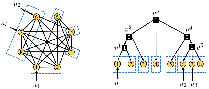
Figure 3: Sibling partition and control nodes in a cograph and its cotree.

Proposition 10

Any permutation that permutes two nodes of a cell in a sibling partition of a cograph $G$ and fixes all other nodes is an automorphism of $G$.

Proof: Let $\sigma:V\rightarrow V$ be a permutation such that for the two nodes $i,j\in V$, $\sigma(i)=j$ and $\sigma(j)=i$, and for any node $k\notin\{i,j\}$, $\sigma(k)=k$. Then, the edge $\{k,l\}\in E$ is mapped to itself if either $k,l\notin\{i,j\}$ or $k=i$ and $l=j$. Otherwise, any edge $\{i,k\}\in E$ (respectively, $\{j,k\}\in E$), where $k\notin\{i,j\}$, is mapped to $\{\sigma(i),\sigma(k)\}=\{j,k\}$ (respectively, $\{\sigma(j),\sigma(k)\}=\{i,k\}$). Moreover, since $i$ and $j$ are siblings, $k\in N(i)$ if and only if $k\in N(j)$. Thus, for any edge $\{l,z\}\in E$, where $l,z\in V$, we have $\{\sigma(l),\sigma(z)\}\in E$, and hence, $\sigma$ is an automorphism of $G$. $\blacksquare$

Remark 11

Note that the sibling partition $\pi_{\mathrm{sib}}(G)$ is an equitable partition of a cograph in the sense that all nodes in any cell of $\pi_{\mathrm{sib}}(G)$ have the same neighbors in other cells (for more information about equitable partitions, one may refer to [12, 5, 17]).

The next theorem, which is the main result of this paper, presents a procedure for selecting a minimal set of control nodes in a Laplacian network defined on a cograph. In fact, in order to break the symmetries in every cell $\mathbf{C}_{i}$ of size $m_{i}$ in the sibling partition of a cograph, one needs to choose $m_{i}-1$ control nodes from that cell. Next, we show that the resulting set of control nodes ensures the network controllability.

Theorem 12

Consider a network defined on a connected cograph $G$ of size $n>1$ with dynamics (1). Let $\pi_{\mathrm{sib}}(G)=\{\mathbf{\mathbf{C}}_{1},\ldots,\mathbf{C}_{p}\}$, where $|\mathbf{C}_{i}|=m_{i}$, $1\leq i\leq p$. Then, the minimum number of control nodes rendering the network controllable is $n-p$. Moreover, a control node set of size $n-p$ should be chosen by selecting $m_{i}-1$ nodes from any cell $\mathbf{C}_{i}$ of $\pi_{\mathrm{sib}}(G)$, $1\leq i\leq p$.

Proof: First, assume that the network is controllable, yet $|V_{C}|<n-p$. Then, there is a cell $\mathbf{C}_{k}$, for some $1\leq k\leq p$, at least two nodes of which, say $i$ and $j$, are not in $V_{C}$. Now, consider a permutation $\sigma$ of $G$ that permutes $i$ and $j$ and fixes all other nodes of the graph (including all control nodes). Based on Proposition 10, $\sigma$ is an automorphism of $G$, and thus from Proposition 2, the system is uncontrollable, contradicting the assumption.

Now, consider the cotree $\mathcal{T}$ with the root $r$, associated with $G$. Let $v^{1},\ldots,v^{h}$ be the internal nodes of $\mathcal{T}$. Then from Theorem 5, the nontrivial spectrum and modal matrix of $G$ are obtained by (4) and (5). Let $V_{C}$ be obtained by choosing $m_{i}-1$ nodes from any cell $\mathbf{C}_{i}$, $1\leq i\leq p$; however, assume that the network is not controllable. Therefore, from Proposition 1, there should be a nonzero eigenvector $\nu$ associated with the eigenvalue $\lambda$, where $\nu^{T}B=0$. For $i_{j}\in\{1,\ldots,h\}$, $1\leq j\leq k$, assume that $\lambda_{i_{j}}=\lambda$, where $\lambda_{i_{j}}=\lambda_{\mathrm{upd}}^{r}(v^{i_{j}})$. Now define $\mathcal{V}=[\mathcal{V}^{(i_{1})},\ldots,\mathcal{V}^{(i_{k})}]$, where for $1\leq j\leq k$, $\mathcal{V}^{(i_{j})}=\mathcal{V}_{\mathrm{upd}}^{r}(v^{i_{j}})$, and note that $L(G)\mathcal{V}=\lambda\mathcal{V}$. Hence, for some nonzero $\alpha\in\mathbb{R}^{n}$, one can write $\nu=\mathcal{V}\alpha$. Moreover, note that from Lemma 7 and Proposition 8, for $1\leq j<l\leq k$, we have $\mathcal{L}(v^{i_{j}})\cap\mathcal{L}(v^{i_{l}})=\emptyset$. This simply implies that $B^{T}\mathcal{V}$ is full rank if and only if $B^{T}\mathcal{V}^{(i_{j})}$, for every $1\leq j\leq k$, is full rank.

Now, we want to prove that by choosing this $V_{C}$, $B^{T}\mathcal{V}^{(i_{j})}$ is full rank. Let $v^{i_{j}}$ be an internal node of $\mathcal{T}$ with $\mathcal{C}(v^{i_{j}})=V_{\mathrm{int}}\cup V_{\mathrm{leaf}}$, where $V_{\mathrm{int}}$ (respectively, $V_{\mathrm{leaf}}$) is the set of children of $v^{i_{j}}$ that are internal nodes (respectively, leaves) of $\mathcal{T}$. Let $u\in V_{\mathrm{int}}$. Then, from Proposition 6, the cograph $G_{(u)}$ has at least two nodes which are siblings. Accordingly, by choosing this set of control nodes $V_{C}$, there is a leaf $w\in\mathcal{L}(u)$ such that $w\in V_{C}$. Moreover, if $V_{\mathrm{leaf}}\neq\emptyset$, it includes the leaves of $\mathcal{T}$ with the same parent $v^{i_{j}}$, and thereby, for some $1\leq k\leq p$, $V_{\mathrm{leaf}}=\mathbf{C}_{k}$, where $\mathbf{C}_{k}$ is a cell of the sibling partition, and $|V_{\mathrm{leaf}}|=m_{k}$. Hence, for the internal node $v^{i_{j}}$, $V_{C}$ includes one leaf of any internal node $u\in V_{\mathrm{int}}$. Moreover, it includes $m_{k}-1$ nodes of $V_{\mathrm{leaf}}$. Therefore, for every internal node $v^{i_{j}}$, $V_{C}$ includes an associated set $\mathcal{S}$ chosen by Procedure I, and thus Lemma 9 implies that $B^{T}\mathcal{V}_{\mathrm{upd}}^{r}(v^{i_{j}})$ is full rank. Accordingly, $B^{T}\mathcal{V}$ is full rank, and if for some $\alpha\in\mathbb{R}^{n}$, $B^{T}\mathcal{V}\alpha=0$, we should have $\alpha=0$. In other words, $\nu=0$, contradicting the assumption. Then, the network is controllable; note that $|V_{C}|=n-p$. Thus, the minimum number of control nodes rendering the network controllable is $n-p$, completing the proof. $\blacksquare$

For the necessity part of Theorem 12, we proved that the sibling partition of a cograph is an equitable partition, where in order to break the structural symmetries, one needs to control at least all nodes of any cell except one. However, the sufficiency part of the theorem is more challenging and intricate; it holds only due to the specific structure of a cograph. To better understand the intricacy of this problem, consider a graph with a nontrivial automorphism in Fig. 4. One may expect that by choosing any of nodes 1 or 2 as the single control node, the controllability of this graph is ensured; while in [47], it has been shown that this graph is completely uncontrollable. Thus, breaking all symmetries in a general graph does not necessarily ensure its controllability.

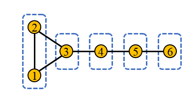
Figure 4: Equitable partition in a completely uncontrollable graph.

Now, let $n_{C}$ be the number of different sets of control nodes with the minimum size from which a network defined on a cograph is controllable. Then, from Theorem 12, $n_{C}=\Pi_{i=1}^{p}m_{i}$.

Example: Consider a network with dynamics (1) defined on the cograph in Fig. 3. By choosing a single node from cell $\mathbf{C}_{1}$, and two nodes from cell $\mathbf{C}_{5}$, the controllability of the network is ensured. For example, the network is controllable from $V_{C_{1}}=\{1,6,7\}$, $V_{C_{2}}=\{2,6,7\}$, $V_{C_{3}}=\{1,6,8\}$, $V_{C_{4}}=\{2,6,8\}$, $V_{C_{5}}=\{1,7,8\}$, and $V_{C_{6}}=\{2,7,8\}$.

IV-A Controllability of Subclasses of Cographs

In this part, using Theorem 12, we derive controllability conditions for some known subclasses of cographs.

A complete graph $K_{n}$ can be represented as $K_{n}=K_{1}*\ldots*K_{1}$. By considering the corresponding cotree, one can see that $\pi_{\mathrm{sib}}(K_{n})=\{\{1,\ldots,n\}\}$. Thus, a network with Laplacian dynamics (1) and the graph $K_{n}$ is controllable from at least $n-1$ nodes; a result which was established by other methods previously (e.g., see for example [15, 12]).

Proposition 13

A Laplacian network (with dynamics (1)) defined on a complete bipartite graph $K_{n_{1},n_{2}}$ is controllable from at least $n_{1}+n_{2}-2$ control nodes.

Proof: Let $V_{1}=\{v_{1},\ldots,v_{n_{1}}\}$ and $V_{2}=\{u_{1},\ldots,u_{n_{2}}\}$, and define $G_{1}=(V_{1},\emptyset)$, $G_{2}=(V_{2},\emptyset)$. Then we have $K_{n_{1},n_{2}}=G_{1}*G_{2}$, implying that $\pi_{\mathrm{sib}}(K_{n_{1},n_{2}})=\{\{v_{1},\ldots,v_{n_{1}}\},\{u_{1},\ldots,u_{n_{2}}\}\}$. By Theorem 12, the result is now immediate . $\blacksquare$

In what follows, we consider an important subclass of cographs, namely threshold graphs, and as a byproduct of Theorem 12, we re-establish the same result of [42, 43] by using a different approach.

Consider a threshold graph $G=(V,E)$ of size $n$. Let $\mathcal{T}=(V^{\mathcal{T}},E^{\mathcal{T}})$ be its cotree with $v^{1},\ldots,v^{h}$ as the internal nodes. From the aforementioned results, one can infer the following properties for a threshold graph, which may not hold for a general cograph:

1. Any internal node of $\mathcal{T}$ has at least one child that is a leaf.

2. For any two internal nodes $v^{i},v^{j}\in V^{\mathcal{T}}$, $\lambda_{\mathrm{upd}}^{r}(v^{i})\neq\lambda_{\mathrm{upd}}^{r}(v^{j})$.

3. If $v^{i}$, $1\leq i\leq h$, is labeled as 1 (respectively, 0), then for any $k\in V$ whose corresponding leaf is a child of $v^{i}$, we have $d(k)=\lambda_{\mathrm{upd}}^{r}(v^{i})-1$ (respectively, $d(k)=\lambda_{\mathrm{upd}}^{r}(v^{i})$).

4. Consider some internal node $w$ whose children–that are leaves–are indexed from $i_{1}$ to $i_{2}$. Then, the new modal matrix at $w$ is

   $$\scriptsize\mathcal{V}_{\mathrm{new}}(w)=\begin{bmatrix}1&1&\ldots&1\\ \vdots&\vdots&\ddots&\vdots\\ -n_{1}&1&\ldots&1\\ 0&-n_{1}+1&\ldots&1\\ \vdots&\vdots&\ddots&\vdots\\ 0&0&\ldots&-n_{2}\end{bmatrix},$$

   where $n_{1}=1$ if $w$ is $v^{1}$, and otherwise $n_{1}=i_{1}-1$. Also, $n_{2}=i_{2}-1$.

Property 1 follows from the definition of a threshold graph. Furthermore, Property 2 is inferred from Lemma 7, and Properties 3 and 4 result from Theorem 5. Thus, there is a direct relationship between the degree sequence of a threshold graph and its set of eigenvalues. However, a general cograph might have some internal nodes, none of whose children is a leaf. As such, the degree sequence of a cograph does not reflect its spectrum in a transparent manner. Moreover, a general cograph might have internal nodes that are associated with the same eigenvalue, making its controllability analysis complicated.

The next result immediately follows from Theorem 1.2.4 of [39]; it states that in a threshold graph, two nodes are siblings if and only if they are of the same degree.

Theorem 14

Given a threshold graph $G=(V,E)$, two nodes $i,j\in V$ are siblings if and only if $d(i)=d(j)$.

Now, in a threshold graph $G=(V,E)$, partition $V$ into the cells $\mathbf{C}_{1},\ldots,\mathbf{C}_{h}$, where for any $i,j\in V$, we have $d(i)=d(j)$ if and only if for some $1\leq k\leq h$, $i,j\in\mathbf{C}_{k}$. The partition $\pi_{\mathrm{deg}}=\{\mathbf{C}_{1},\ldots,\mathbf{C}_{h}\}$ is called a degree partition. Let $m_{i}=|\mathbf{C}_{i}|$, for $1\leq i\leq h$. The next result that follows immediately from Theorems 12 and 14 is the same as the result of [42, 43] for a general threshold graph, obtained by adopting a different approach.

Corollary 15

For the controllability of a network defined on a threshold graph with dynamics (1) and the input matrix (2), at least $n-h$ control nodes are needed, which should be chosen by selecting $m_{i}-1$ nodes from any cell $\mathbf{C}_{i}$, $1\leq i\leq h$, of its degree partition.

V Conclusions

In this work, we characterized the controllability of Laplacian networks defined over cographs in terms of certain graph-theoretic conditions. These characterizations are built upon the intricate correspondance between the inherent structural modularity of cographs, with respect to join and union operation, and its modal properties. Moreover, we used the proposed framework to provide a procedure for selecting a set of control nodes guaranteeing the controllability of cograph networks. In particular, we demonstrated that the minimum number of control nodes rendering a cograph controllable is the difference between its size and the number of cells of its sibling partition. It was also revealed that the larger a cell of sibling nodes, the larger the multiplicity of one of the eigenvalues associated with the Laplacian matrix; such multiplicities are often associated with higher degrees of symmetry in the network. We then applied our results to certain subclasses of cographs such as threshold graphs, and by adopting a different approach, presented conditions that ensure their controllability. As one of the future research topics, in order to minimize the number of independent controllers of a cograph, one can consider the more general case where the input matrix $B$ is binary with more than one nonzero entry at each column. Furthermore, controllability analysis of weighted or directed cographs can be taken into account.

References

- [1] H. G. Tanner, “On the controllability of nearest neighbor interconnections,” in Proc. 43rd IEEE Conf. on Decision and Control, vol. 3, 2004, pp. 2467–2472.
- [2] S. S. Mousavi, M. Haeri, and M. Mesbahi, “On the structural and strong structural controllability of undirected networks,” IEEE Trans. Automat. Contr., vol. 63, no. 7, pp. 2234–2241, 2018.
- [3] ——, “Robust strong structural controllability of networks with respect to edge additions and deletions,” in American Control Conf., 2017, pp. 5007–5012.
- [4] S. S. Mousavi, A. Chapman, M. Haeri, and M. Mesbahi, “Null space strong structural controllability via skew zero forcing sets,” in 2018 European Control Conf., 2018, pp. 1845–1850.
- [5] S. Zhang, M. Cao, and M. K. Camlibel, “Upper and lower bounds for controllable subspaces of networks of diffusively coupled agents,” IEEE Trans. Automat. Contr., vol. 59, no. 3, pp. 745–750, 2014.
- [6] Z. Ji, H. Lin, and H. Yu, “Protocols design and uncontrollable topologies construction for multi-agent networks,” IEEE Trans. Automat. Contr., vol. 60, no. 3, pp. 781–786, 2015.
- [7] A. Yazıcıoğlu, W. Abbas, and M. Egerstedt, “Graph distances and controllability of networks,” IEEE Trans. Automat. Contr., vol. 61, no. 12, pp. 4125–4130, 2016.
- [8] Z. Ji and H. Yu, “A new perspective to graphical characterization of multiagent controllability,” IEEE Trans. Cybernetics, vol. 47, no. 6, pp. 1471–1483, 2017.
- [9] R. Olfati-Saber, J. A. Fax, and R. M. Murray, “Consensus and cooperation in networked multi-agent systems,” Proc. IEEE, vol. 95, no. 1, pp. 215–233, 2007.
- [10] Z. Ji, Z. Wang, H. Lin, and Z. Wang, “Interconnection topologies for multi-agent coordination under leader–follower framework,” Automatica, vol. 45, no. 12, pp. 2857–2863, 2009.
- [11] M. Mesbahi and M. Egerstedt, Graph Theoretic Methods in Multiagent Networks. Princeton, NJ: Princeton Univ. Press, 2010.
- [12] A. Rahmani, M. Ji, M. Mesbahi, and M. Egerstedt, “Controllability of multi-agent systems from a graph-theoretic perspective,” SIAM J. Control and Optimiz., vol. 48, no. 1, pp. 162–186, 2009.
- [13] A. Chapman and M. Mesbahi, “State controllability, output controllability and stabilizability of networks: A symmetry perspective,” in Proc. 54th IEEE Conf. on Decision and Control, Osaka, 2015, pp. 4776–4781.
- [14] M. Egerstedt, S. Martini, M. Cao, K. Camlibel, and A. Bicchi, “Interacting with networks: How does structure relate to controllability in single-leader, consensus networks?” IEEE Control Syst. Mag., vol. 32, no. 4, pp. 66–73, 2012.
- [15] S. Zhang, M. K. Camlibel, and M. Cao, “Controllability of diffusively-coupled multi-agent systems with general and distance regular coupling topologies,” in Proc. 50th IEEE Conf. on Decision and Control and Eur. Control Conf., Orlando, FL, 2011, pp. 759–764.
- [16] M. Cao, S. Zhang, and M. K. Camlibel, “A class of uncontrollable diffusively coupled multiagent systems with multichain topologies,” IEEE Trans. Automat. Contr., vol. 58, no. 2, pp. 465–469, 2013.
- [17] C. O. Aguilar and B. Gharesifard, “Almost equitable partitions and new necessary conditions for network controllability,” Automatica, vol. 80, pp. 25–31, 2017.
- [18] A. Y. Yazicioglu, W. Abbas, and M. Egerstedt, “A tight lower bound on the controllability of networks with multiple leaders,” in Proc. 51st IEEE Conf. on Decision and Control, Maui, HI, 2012, pp. 1978–1983.
- [19] G. Parlangeli and G. Notarstefano, “On the reachability and observability of path and cycle graphs,” IEEE Trans. Automat. Contr., vol. 57, no. 3, pp. 743–748, 2012.
- [20] S. S. Mousavi and M. Haeri, “Controllability analysis of networks through their topologies,” in Proc. 55th IEEE Conf. on Decision and Control, 2016, pp. 4346–4351.
- [21] X. Liu and Z. Ji, “Controllability of multiagent systems based on path and cycle graphs,” Int. J. Robust Nonlinear Control, vol. 28, no. 1, pp. 296–309, 2018.
- [22] M. Nabi-Abdolyousefi and M. Mesbahi, “On the controllability properties of circulant networks,” IEEE Trans. Automat. Contr., vol. 58, no. 12, pp. 3179–3184, 2013.
- [23] S.-P. Hsu, “A necessary and sufficient condition for the controllability of single-leader multi-chain systems,” Int. J. Robust Nonlinear Control, vol. 27, no. 1, pp. 156–168, 2017.
- [24] G. Notarstefano and G. Parlangeli, “Controllability and observability of grid graphs via reduction and symmetries,” IEEE Trans. Automat. Contr., vol. 58, no. 7, pp. 1719–1731, 2013.
- [25] Z. Ji, H. Lin, and H. Yu, “Leaders in multi-agent controllability under consensus algorithm and tree topology,” Syst. Control Lett., vol. 61, no. 9, pp. 918–925, 2012.
- [26] T. N. Tran and A. Chapman, “Generalized graph product: Spectrum, trajectories and controllability,” in Proc. 57th IEEE Conf. on Decision and Control and Eur. Control Conf., 2018, pp. 5358–5363.
- [27] Z. Ji, T. Chen, and H. Yu, “A design method for controllable topologies of multi-agent networks,” in Proc. 35th Chinese Control Conf. (CCC), 2016, pp. 7578–7584.
- [28] D. G. Corneil, H. Lerchs, and L. S. Burlingham, “Complement reducible graphs,” Discrete Applied Math., vol. 3, no. 3, pp. 163–174, 1981.
- [29] R. Merris, “Laplacian graph eigenvectors,” Linear Alg. and its Applic., vol. 278, no. 1-3, pp. 221–236, 1998.
- [30] T. Bıyıkoglu, J. Leydold, and P. F. Stadler, Laplacian Eigenvectors of Graphs. Lecture Notes in Mathematics. New York, NY: Springer, 2007.
- [31] D. Corneil, Y. Perl, and L. Stewart, “Cographs: recognition, applications and algorithms,” Congressus Numerantium, vol. 43, pp. 249–258, 1984.
- [32] D. G. Corneil, Y. Perl, and L. K. Stewart, “A linear recognition algorithm for cographs,” SIAM J. Computing, vol. 14, no. 4, pp. 926–934, 1985.
- [33] M. Hellmuth, M. Hernandez-Rosales, K. T. Huber, V. Moulton, P. F. Stadler, and N. Wieseke, “Orthology relations, symbolic ultrametrics, and cographs,” J. math. biology, vol. 66, no. 1-2, pp. 399–420, 2013.
- [34] M. Habib and C. Paul, “A simple linear time algorithm for cograph recognition,” Discrete Applied Math., vol. 145, no. 2, pp. 183–197, 2005.
- [35] Q. Cheng, P. Berman, R. Harrison, and A. Zelikovsky, “Efficient alignments of metabolic networks with bounded treewidth,” in Data Mining Workshops (ICDMW), 2010 IEEE International Conference on, 2010, pp. 687–694.
- [36] S. Jia, L. Gao, Y. Gao, J. Nastos, Y. Wang, X. Zhang, and H. Wang, “Defining and identifying cograph communities in complex networks,” New J. Phys., vol. 17, no. 1, p. 013044, 2015.
- [37] S. Jia, L. Gao, Y. Gao, J. Nastos, X. Wen, X. Huang, and H. Wang, “Viewing the meso-scale structures in protein-protein interaction networks using 2-clubs,” IEEE Access, vol. 6, pp. 36 780–36 797, 2018.
- [38] S. Saha, N. Ganguly, A. Mukherjee, and T. Krueger, “Intergroup networks as random threshold graphs,” Phys. Rev. E, vol. 89, no. 4, p. 042812, 2014.
- [39] N. V. Mahadev and U. N. Peled, Threshold graphs and related topics. Elsevier, 1995, vol. 56.
- [40] C. O. Aguilar and B. Gharesifard, “Laplacian controllability classes for threshold graphs,” Linear Alg. and its Applic., vol. 471, pp. 575–586, 2015.
- [41] S.-P. Hsu, “Controllability of the multi-agent system modeled by the threshold graph with one repeated degree,” Syst. Control Lett., vol. 97, pp. 149–156, 2016.
- [42] S. S. Mousavi, M. Haeri, and M. Mesbahi, “Controllability analysis of threshold graphs and cographs,” in 2018 European Control Conf., 2018, pp. 1–6.
- [43] S.-P. Hsu, “Minimal laplacian controllability problems of threshold graphs,” IET Control Theory & Applications, 2019.
- [44] C. Godsil and G. F. Royle, Algebraic graph theory. Springer Science & Business Media, 2013, vol. 207.
- [45] P. L. Hammer and A. K. Kelmans, “Laplacian spectra and spanning trees of threshold graphs,” Disc. Appl. Math., vol. 65, no. 1-3, pp. 255–273, 1996.
- [46] E. D. Sontag, Mathematical Control Theory: Deterministic Finite Dimensional Systems. New York: Springer Verlag, 1998.
- [47] C. O. Aguilar and B. Gharesifard, “Graph controllability classes for the laplacian leader-follower dynamics,” IEEE Trans. Automat. Contr., vol. 60, no. 6, pp. 1611–1623, 2015.