Theory of Friedel oscillations in monolayer graphene and group-VI dichalcogenides in a magnetic field

Abstract

Friedel oscillations (FO) of electron density caused by a delta-like neutral impurity in two-dimensional (2D) systems in a magnetic field are calculated. Three 2D cases are considered: free electron gas, monolayer graphene and group-VI dichalcogenides. An exact form of the renormalized Green’s function is used in the calculations, as obtained by a summation of the infinite Dyson series and regularization procedure. Final results are valid for large ranges of potential strengths $V_{0}$, electron densities $n_{e}$, magnetic fields $B$ and distances from the impurity $r$. Realistic models for the impurities are used. The first FO of induced density in WS₂ are described by the relation $\Delta n({\bm{r}})\propto\sin(2\pi r/T_{FO})/r^{2}$, where $T_{FO}\propto 1/\sqrt{E_{F}}$. For weak impurity potentials, the amplitudes of FO are proportional to $V_{0}$. For attractive potentials and high fields the total electron density remains positive for all $r$. On the other hand, for low fields, repulsive potentials and small $r$, the total electron density may become negative, so that many-body effects should be taken into account.

I Introduction

Disturbing a free-electron gas in a metal or a semiconductor with an impurity gives rise to the Friedel oscillation (FO) of electron density Friedel1952 . In the vicinity of the impurity, usually a foreign atom embedded in the host material or a vacancy, the electron density oscillates

$$n(\bm{r})\simeq n_{0}+\delta n\frac{\sin(2k_{F}r+\phi)}{r^{D}},$$ (1)

where $n_{0}$ is the electron gas density in the absence of impurity, $\delta n$ is the magnitude of induced density, $k_{F}$ is the Fermi vector of the electron gas, $D$ is dimensionality of the system, and $\phi$ is the phase shift.

Physically, FO result from a redistribution of electrons caused by the potential of the impurity. Because in a metal or a semiconductor only electrons with energies near to the Fermi level can participate in the redistribution, the induced density is characterized by the wave vector $k\simeq k_{F}$. Since their discovery in 1952, FO have been investigated both theoretically and experimentally in many systems. For a recent review of this subject see Ref. Villain2016 .

Friedel oscillations were investigated in monolayer Cheianov2006 and bilayer graphene Hwang2008 with the use of ${\bm{k}}\cdot{\bm{p}}$ and tight binding methods Bena2008 ; Bacsi2010 . Recently, they were analyzed in hexagonal-lattices systems of group-VI dichalogenides Scholz2013 and black phosphorous Zou2016 . In all above papers the oscillations were treated in absence of external fields. However, FO also exist in the presence of a magnetic field, and their theoretical investigation in 2D electron gases is a subject of the present work. Since the problem of FO in a magnetic field is less frequently discussed in the literature, we present a short review of this subject.

The first attempts to analyze FO in a magnetic field were carried out by Rensink Rensink1968 , Glasser Glasser1969 ; Glasser1970 and Horing Horing1969a ; Horing1969b who considered 3D electron gas and delta-like or screened Coulomb impurities. The main conclusions of these papers were: i) for weak perturbations by an external potential, FO follow formula (1) with $\phi=0$, ii) there is a qualitative difference between oscillations in directions parallel and perpendicular to magnetic field, iii) in strong quantizing fields the induced density decays exponentially, iv) FO induced by the delta-like potential are similar to those induced by the short-range screened Coulomb potential.

There exist several papers treating FO in a magnetic field in different systems. Sedrakyan et al. Sedrakyan2007 considered the impact of magnetic field on a high-density electron gas and found a correction to the electrostatic potential and an additional distance-dependent phase shift. Sharma and Reddy Sharma2011 considered electronic screening at densities of relevance to neutron star crusts and found that the screened potential between two static charges exhibits long-range FO parallel to magnetic field that can possibly create rod-like structures in the magnetar crusts. Simion and Giuliani Simion2005 treated FO in 2D electron gas for electrons occupying the lowest Landau level. Horing and Liu Horing2009 treated FO arising from the delta potential in monolayer graphene, but they were faced with divergencies in the one-electron Green’s function. Bena Bena2016 calculated FO in monolayer graphene in a magnetic field in the lowest order of Born approximation. A problem of free electrons in 2D and 3D interacting with point impurities in a magnetic field was analyzed by Avishai et al. Avishai1993 using an approach similar to that presented in our paper. However, among properties calculated in Ref. Avishai1993 the authors did not consider the Friedel oscillations of electron density in modern materials.

Our work has three purposes. First, we want to extend the results by Rensink, Glasser and Horing Rensink1968 ; Glasser1969 ; Glasser1970 ; Horing1969a ; Horing1969b to 2D electron systems based on honeycomb lattices as, e.g., monolayer graphene and group-VI dichalogenides MoS₂ or WS₂. Second, being inspired by the approach of Horing and Liu Horing2009 , we apply a regularization method used in the quantum field theory to handle the divergencies of one electron Green’s function. This method allows us to sum up exactly the Born series for the Green’s function of 2D electrons in a magnetic field in the presence of a delta-like impurity for arbitrary strength of the potential. Third, we to calculate FO going beyond the perturbation scheme by using the exact one-electron Green’s functions. We hope that theoretical results for materials with 2D honeycomb lattice will encourage experimental observation of FO in graphene and group-VI dichalogenides in a magnetic field.

The crucial point of our approach is a possibility of exact summation of the Born series, which requires isolation of the divergent part in the one-electron Green’s function (GF) and a renormalization of the coupling constant. This approach was successfully applied to high field magneto-resistance at low temperatures in 3D systems by Gerhards and Hajdu Gerhards1971 and we adopted their method to the 2D electron gas. It turns out that, for realistic material parameters, energies and magnetic fields, the renormalized potential of the impurity is close to the original one, which justifies the regularization procedure. However, the proper regularization of the one-electron GF, as described in our paper, requires knowledge of the one-electron GF and its analytical behavior at the origin. For this reason, our approach could not be used in the past when this feature was not known. Below we give a short review of works related to this subject.

Some years ago Dodonov et al. Dodonov1975 calculated stationary GF for a free 2D electron in a homogeneous magnetic field and obtained analytical results in terms of the Whittaker functions. Similar problems were recently investigated for low-dimensional systems Gusynin1995 ; Gorbar2002 ; Murguia2010 and GF was obtained as infinite sums of Laguerre polynomials. Horing and Liu Horing2009 obtained a propagator as an infinite sum and, alternatively, as the second solution of Bessel wave equation. A closed form of the propagator in monolayer graphene in terms of the confluent hypergeometric function was obtained by Pyatkovskiy and Gusynin Pyatkovskiy2011 and Gamayun et al. Gamayun2011 . The present authors Rusin2011 calculated the propagator in monolayer and bilayer graphene and obtained results in terms of Whittaker functions. Ardenghi et al. Ardenghi2015 calculated GF of graphene taking into account corrections caused by the coherent potential approximation, while Gutierrez-Rubio et al. Rubio2016 calculated numerically magnetic susceptibility of graphene and MoS₂ within the GF formalism. Recently, the present authors published online the results for one electron GF in a magnetic field for group-VI dichalogeinides Rusin2016 , and Horing Horing2017 considered the one-electron GF in the same materials in position and momentum representations.

Our approach is based on the ${\bm{k}}\cdot{\bm{p}}$ theory of graphene and group-VI dichalogeinides in the vicinity of ${\bm{K}}$ and ${\bm{K}}^{\prime}$ points of the Brillouin zone (BZ). We assume a non-interacting electron gas at $T=0$. The broadening parameters of GF are taken from experimental values reported in the literature and we use realistic values of impurity potentials. For graphene we take a model potential of the nitrogen-like impurity which is a frequent dopant in this material. Since we were unable to find analogous model potential for group-VI dichalogeinides, we take for this case potentials of nickel atom and a vacancy used in ab-initio calculations of high-T_c superconductors. Finally, we mention that FO in WS₂ in a magnetic field calculated in the parabolic-band approximation follow exact results of Dodonov et al. Dodonov1975 for the GF of the 2D electron gas, while the calculations of FO in monolayer graphene follow the results obtained by the present authors in Ref. Rusin2011 .

Our paper is organized as follows. In Section II we introduce the theory of FO in 2D electron systems including a detailed description of the regularization procedure. Section III contains our main results and Section IV their discussion. The paper is concluded by the Summary. In Appendices we discuss auxiliary problems related to our main subject.

II Theory

We describe the theory of density oscillations of a non-interacting electron gas in 2D systems in the presence of a neutral delta-like impurity in a constant magnetic field. These oscillations are similar to FO of a 3D electron gas in the presence of an impurity in absence of fields. The density of electron gas is calculated from GF of the system consisting of free electrons in a magnetic field and a neutral impurity. We analyze four models: 2D gas of noninteracting electrons, electron gas in the conduction bands of monolayer graphene and in group-VI dichalogenides (e.g. WS₂) in the parabolic and non-parabolic approximations.

The calculations for the four systems are similar but for 2D electron gas GFs entering to the calculations are scalars while for remaining systems GFs are block-diagonal $4\times 4$ or $8\times 8$ matrices. The presence of matrices introduces complications in intermediate stages and final formulas, but it does not change main conclusions about the physical nature of FO in a magnetic field. For this reason we present detailed calculations for 2D electron gas, while for the other systems we only quote the main steps of calculations and final results.

II.1 2D electron gas in a magnetic field

In the presence of a magnetic field the Hamiltonian for a 2D electron gas is: $\hat{H}=(\hat{\bm{p}}+e{\bm{A}})^{2}/(2m_{0})$, where $\hat{\bm{p}}$ is electron’s momentum, ${\bm{A}}$ is vector potential, $m_{0}$ is electron mass and $e$ is its charge ($e>0$). In the Landau gauge ${\bm{A}}=(-By,0)$. Let $L=\sqrt{\hbar/eB}$ be the magnetic radius and $\xi=y/L-k_{x}L$. Defining the standard raising and lowering operators for the harmonic oscillator: $\hat{a}=(\xi+\partial/\partial\xi)/\sqrt{2}$ and $\hat{a}^{+}=(\xi-\partial/\partial\xi)/\sqrt{2}$ we have

$$\hat{H}=\hbar\omega_{c}(\hat{a}^{+}\hat{a}+1/2),$$ (2)

with $\omega_{c}=eB/m_{0}$. The eigenstates of $\hat{H}$ are $E_{n}=\hbar\omega(n+1/2)$, where $n=0,1,\ldots$ is the Landau level number, and the eigenstates of $\hat{H}$ are:

$$\Psi_{nk_{x}}({\bm{\rho}})=\frac{e^{ik_{x}x}}{\sqrt{2\pi}}\phi_{n}(\xi),$$ (3)

where ${\bm{\rho}}=(x,y)$, $\phi_{n}(\xi)=(1/\sqrt{L})C_{n}{\rm H}_{n}(\xi)e^{-\xi^{2}/2}$, in which ${\rm H}_{n}(\xi)$ are the Hermite polynomials, and $C_{n}=1/\sqrt{2^{n}n!\sqrt{\pi}}$ are the normalization coefficients. The electron spin is omitted.

The GF for the Hamiltonian (2) is $\hat{g}_{2D}=(E-\hat{H})^{-1}$. In the position representation this operator reads

$$\hat{g}_{2D}({\bm{\rho}}_{1},{\bm{\rho}}_{2})=\sum_{n=0}^{\infty}\int_{-\infty}^{\infty}\frac{\phi_{n}(x,\xi_{1})\phi_{n}^{*}(x^{\prime},\xi_{2})}{E-E_{n}}dk_{x}.$$ (4)

Performing the integration over $k_{x}$ (see Appendix A) one obtains

$$\hat{g}_{2D}({\bm{\rho}}_{1},{\bm{\rho}}_{2},\bar{\cal E}) = -A(\omega_{c})\sum_{n=0}^{\infty}\frac{L_{n}(r^{2})}{n+1/2-\bar{\cal E}},$$ (5)

$$A(\omega) = \frac{e^{-r^{2}/2+i\chi}}{2\pi\hbar\omega L^{2}},$$ (6)

where $\bar{\cal E}=E/(\hbar\omega_{c})$, $r^{2}=({\bm{\rho}}_{1}-{\bm{\rho}}_{2})^{2}/(2L^{2})$, $\chi=(x_{1}-x_{2})(y_{1}+y_{2})/2L^{2}$ is the gauge-dependent phase factor, and $L_{n}(z)$ are the Laguerre polynomials. The sum in Eq. (5) can be expressed in terms of the Whittaker functions Dodonov1975 . Introducing notation $\hat{g}_{{\bm{1}},{\bm{2}}}=\hat{g}_{2D}({\bm{\rho}}_{1},{\bm{\rho}}_{2},\bar{\cal E})$ one has

$$\hat{g}_{{\bm{1}},{\bm{2}}}=-\frac{e^{i\chi}}{2\pi\hbar\omega_{c}L^{2}|r|}{\cal W}_{\bar{\cal E}}(r^{2}),$$ (7)

where we define: ${\cal W}_{\kappa}(z)=\Gamma(1/2-\kappa)W_{\kappa,0}(z)$, while $\Gamma(z)$ and $W_{\kappa,0}(z)$ are the Euler gamma and the Whittaker functions GradshteinBook , respectively. Note the change of sign in Eq. (7) compared with Refs. Dodonov1975 ; Rusin2011 .

II.2 Born series summation and regularization procedure

Consider the Dyson equation for a point-like impurity potential $V(\bm{\rho})=V_{0}\delta(\bm{\rho}-\bm{\rho}_{0})$, where ${\bm{\rho}_{0}}=(x_{0},y_{0})$ is the position of the impurity. Note that $V_{0}$ has the dimensionality of [energy] $\times$ [area]. In the position representation there is

$$\langle{\bm{\rho}}_{1}|\hat{G}|{\bm{\rho}}_{2}\rangle=\langle{\bm{\rho}}_{1}|\hat{g}|{\bm{\rho}}_{2}\rangle+\int\langle{\bm{\rho}}_{1}|\hat{g}|{\bm{\rho}}_{3}\rangle V({\bm{\rho}}_{3})\langle{\bm{\rho}}_{3}|\hat{G}|{\bm{\rho}}_{2}\rangle d^{2}{\bm{\rho}}_{3},$$ (8)

in which $\hat{g}$ is GF of free electron gas in Eq. (7), and $\hat{G}$ is GF of free electron gas in the presence of point-like impurity. Performing in Eq. (8) the integration over ${\bm{\rho}}_{3}$ one has

$$\hat{G}_{{\bm{1}},{\bm{2}}}=\hat{g}_{{\bm{1}},{\bm{2}}}+V_{0}\hat{g}_{{\bm{1}},{\bm{0}}}\hat{G}_{{\bm{0}},{\bm{2}}},$$ (9)

where we used notation: $\hat{g}_{{\bm{1}},{\bm{2}}}=\langle{\bm{\rho}}_{1}|\hat{g}|{\bm{\rho}}_{2}\rangle$ and $\hat{G}_{{\bm{1}},{\bm{2}}}=\langle{\bm{\rho}}_{1}|\hat{G}|{\bm{\rho}}_{2}\rangle$, c.f. Eq. (7). Following Ziman and others ZimanBook ; Koster1954 ; Wolff1961 ; Clogston1962 , the above equation can be solved analytically by setting $\bm{\rho}_{1}\rightarrow{\bm{\rho}_{0}}$. After short algebra one finds

$$\hat{G}_{{\bm{1}},{\bm{2}}}=\hat{g}_{{\bm{1}},{\bm{2}}}+V_{0}\hat{g}_{{\bm{1}},{\bm{0}}}\frac{1}{1-V_{0}\hat{g}_{\bm{0},\bm{0}}}\hat{g}_{{\bm{0}},{\bm{2}}}.$$ (10)

The one-electron GFs in Eq. (10) have poles for energies $E=E_{n}=\hbar\omega_{c}(n+1/2)$, and they diverge for ${\bm{\rho}}_{1}\rightarrow{\bm{\rho}}_{0}$. The standard way to overcome the first problem is to treat the energy as a complex variable by adding or subtracting the imaginary part $\pm i\eta$. Then the resulting GF has finite values at $E=E_{n}$, and the energy levels are smeared around $E_{n}$ over a finite width $\pm\eta/2$. Physically, $\eta$ is a phenomenological constant characterizing scattering processes occurring in real samples. In many cases, as e.g. for the free electron gas in absence of fields, the above receipt allows one to overcome the second problem mentioned above, i.e. the divergence of $\hat{g}_{\bm{0},\bm{0}}$, see Refs. ZimanBook ; Koster1954 ; Wolff1961 ; Clogston1962 .

However, for the GF in Eq. (7) the above procedure is not sufficient, as illustrated below. Turning to Eq. (5) and using notation from Eq. (7) we find

$$\hat{g}_{\bm{0},\bm{0}}=-A(\omega_{c})\sum_{n=0}^{\infty}\frac{1}{n+1/2-\bar{\cal E}+i\eta},$$ (11)

since for ${\bm{\rho}}_{1}\rightarrow{\bm{\rho}}_{2}$ there is ${\bm{r}}={\bm{0}}$ and there is $L_{n}(0)=1$ for all $n$. The series in Eq. (11) is harmonic and it diverges for all $\bar{\cal E}$ and $\eta$. As shown in Appendix D, other methods of smearing GF by using different bell-like forms also lead to divergences in the real part of $\hat{g}_{\bm{0},\bm{0}}$. The above considerations suggest a different way to calculate $\hat{g}_{\bm{0},\bm{0}}$. Below we propose to apply the regularization technique, similar to that outlined in Ref. Gerhards1971 .

Consider the function $\hat{g}_{\bm{\zeta},\bm{0}}$ in Eq. (7) in the limit $|\zeta|\rightarrow 0$. Omitting terms tending to unity we have

$$\hat{g}_{\bm{\zeta},\bm{0}}=-\frac{1}{2\pi\hbar\omega_{c}L^{2}|\zeta|}\Gamma(1/2-\bar{\cal E})W_{\bar{\cal E},0}(\zeta^{2}).$$ (12)

For small arguments there is (see formula 13.14.19 in Ref. dlmf2017 )

$$W_{\kappa,0}(z)=-\frac{\sqrt{z}}{\Gamma(a)}\left[\ln(z)+\psi(a)+2\gamma\right]+O(z^{3/2}\ln(z)),$$ (13)

where $a=1/2-\kappa$, $\psi(z)$ is the digamma function GradshteinBook , and $\gamma\simeq 0.577$ is the Euler-Mascheroni constant. Next, by using Eqs. (12) and (13) we isolate the divergent $\hat{g}_{\bm{\zeta},\bm{0}}^{div}$ and the regular $\hat{g}_{\bm{\zeta},\bm{0}}^{reg}$ parts of $\hat{g}_{\bm{\zeta},\bm{0}}$. There is

$$\hat{g}_{\bm{\zeta},\bm{0}} = \hat{g}_{\bm{\zeta},\bm{0}}^{div}+\hat{g}_{\bm{\zeta},\bm{0}}^{reg},$$ (14)

$$\hat{g}_{\bm{\zeta},\bm{0}}^{div} = \frac{2\ln(\zeta)}{2\pi\hbar\omega_{c}L^{2}},$$ (15)

$$\hat{g}^{reg}\equiv\hat{g}_{\bm{\zeta},\bm{0}}^{reg} = \frac{\psi(1/2-\bar{\cal E})+2\gamma}{2\pi\hbar\omega_{c}L^{2}}.$$ (16)

Note that $\hat{g}_{\bm{\zeta},\bm{0}}^{div}$ diverges logarithmical with $\zeta$. This allows us to treat $\zeta$ as a cut-off parameter, see Discussion. The regular part of $\hat{g}_{\bm{\zeta},\bm{0}}$ in Eq. (16) does not depend on $\zeta$, so we may take: $\hat{g}_{\bm{\zeta},\bm{0}}^{reg}=\hat{g}_{\bm{0},\bm{0}}^{reg}\equiv\hat{g}^{reg}$. The function $\hat{g}^{reg}$ is finite except at the poles $\bar{\cal E}=n+1/2$. By taking the energy as a complex variable we find that, in the vicinity of poles, the density of states (DOS) obtained from $\hat{g}^{reg}$ is accurately described by the Lorentz function, see Appendix C. Equations (14)–(16) agree with results of Avishai et al. Avishai1993 .

From Eqs. (7) and (15)–(16) we obtain

$$\hat{G}_{\bm{1},\bm{2}}=\hat{g}_{\bm{1},\bm{2}}+\hat{g}_{\bm{1},\bm{0}}\frac{V_{0}}{1-V_{0}\hat{g}_{\bm{\zeta},\bm{0}}^{div}-V_{0}\hat{g}^{reg}}\hat{g}_{\bm{0},\bm{2}}.$$ (17)

Now we redefine $V_{0}\rightarrow V_{r}$ in such a way that $\hat{G}_{\bm{1},\bm{2}}$ does not include $\hat{g}_{\bm{\zeta},\bm{0}}^{div}$ explicitly

$$\hat{G}_{\bm{1},\bm{2}}=\hat{g}_{\bm{1},\bm{2}}+\hat{g}_{\bm{1},\bm{0}}\frac{V_{r}}{1-V_{r}\hat{g}^{reg}}\hat{g}_{\bm{0},\bm{2}}.$$ (18)

By using Eqs. (17) and (18) we find

$$V_{r}=\frac{V_{0}}{1-V_{0}\hat{g}_{\bm{\zeta},\bm{0}}^{div}}.$$ (19)

The redefined potential $V_{r}$ depends on the unknown parameter $\zeta\rightarrow 0$, see Eq. (15). However, since the delta-like potential used in our model is an idealized form of realistic potentials of impurities and vacancies or atomic nuclei interacting with the electron gas, one can identify $\zeta$ with an effective range of these potentials. For typical material parameters, see Discussion, there is: $V_{r}\simeq V_{0}$ for impurities, vacancies etc., and $V_{r}\simeq cV_{0}$ for atomic nuclei potentials, with $c$ being on the order of unity. Equations (16), (18), and (19) are the final result of the regularization procedure for 2D electron gas.

II.3 Monolayer graphene

For monolayer graphene in the vicinity of the ${\bm{K}}$ and ${\bm{K}}^{\prime}$ points in BZ the Hamiltonian of electron in a magnetic field is Gusynin2007

$$\hat{H}=u\tau\hat{\sigma}_{x}{\pi}_{x}+u\sigma_{y}\hat{\pi}_{y},$$ (20)

where $u=1\times 10^{6}$ m/s is the electron velocity, $\sigma_{x},\sigma_{y}$ are the Pauli matrices in the standard notation and $\tau=\pm 1$ for the ${\bm{K}}$ and ${\bm{K}}^{\prime}$, respectively. Introducing the raising and lowering operators, and taking $\tau=+1$ (i.e. the ${\bm{K}}$ point) one has

$$\hat{H}=\left(\begin{array}[]{cc}0&-\hbar\Omega\hat{a}\\ -\hbar\Omega\hat{a}^{+}&0\end{array}\right),$$ (21)

where $\Omega=\sqrt{2}u/L$. For both ${\bm{K}}$ and ${\bm{K}}^{\prime}$ points the electron energies are: $E_{n\epsilon}=\epsilon\hbar{\Omega}\sqrt{n}$, $n=0,1,2,\ldots$, and $\epsilon=\pm 1$.

For monolayer graphene in a magnetic field GF operator is a $4\times 4$ block-diagonal matrix: $\hat{g}_{ML}=\left(\begin{array}[]{cc}\hat{g}^{K}&0\\ 0&\hat{g}^{K^{\prime}}\end{array}\right)$, in which $\hat{g}^{K}=\left(\begin{array}[]{cc}\hat{g}^{uu}&\hat{g}^{ul}\\ \hat{g}^{lu}&\hat{g}^{ll}\end{array}\right)$ and $\hat{g}^{K^{\prime}}=\left(\begin{array}[]{cc}\hat{g}^{ll}&-\hat{g}^{lu}\\ -\hat{g}^{ul}&\hat{g}^{uu}\end{array}\right)$ Rusin2011 . The indexes $u$ and $l$ correspond to the upper or the lower components of the eigen-vectors, respectively. Then one has

$$\hat{g}^{uu}({\bm{\rho}},{\bm{\rho}}^{\prime},\bar{\cal E}) = -\frac{\bar{\cal E}e^{i\chi}}{2\pi\hbar\Omega L^{2}|r|}{\cal W}_{\kappa_{u}}(r^{2}),$$ (22)

$$\hat{g}^{ll}({\bm{\rho}},{\bm{\rho}}^{\prime},\bar{\cal E}) = -\frac{\bar{\cal E}e^{i\chi}}{2\pi\hbar\Omega L^{2}|r|}{\cal W}_{\kappa_{l}}(r^{2}),$$ (23)

$$\hat{g}^{ul}({\bm{\rho}},{\bm{\rho}}^{\prime},\bar{\cal E}) = \frac{m_{ul}}{r^{2}}\bar{\cal E}(\hat{g}^{uu}-\hat{g}^{ll}),$$ (24)

where $\kappa_{u}=\bar{\cal E}^{2}-1/2$ and $\kappa_{l}=\bar{\cal E}^{2}+1/2$. In Eq. (24) we defined $m_{ul}=[(y-y^{\prime})+i(x-x^{\prime})]/(\sqrt{2}L)$. For $\hat{g}^{lu}$ one obtains the expression analogous to that for $\hat{g}^{ul}$ in (24), but with $m_{ul}$ replaced by $m_{lu}=[(y^{\prime}-y)+i(x-x^{\prime})]/(L\sqrt{2})$.

For the ${\bm{K}}$ point, the GF of electron gas in monolayer graphene in the presence of a neutral impurity is

$$\hat{G}_{\bm{1},\bm{2}}=\left(\begin{array}[]{cc}\hat{g}^{uu}&\hat{g}^{ul}\\ \hat{g}^{lu}&\hat{g}^{ll}\end{array}\right)_{\!\!\bm{1}\bm{2}}+V_{0}\left(\begin{array}[]{cc}\hat{g}^{uu}&\hat{g}^{ul}\\ \hat{g}^{lu}&\hat{g}^{ll}\end{array}\right)_{\!\!\bm{1}\bm{0}}\left(\hat{I}-V_{0}\hat{g}_{\bm{0},\bm{0}}\right)^{-1}\left(\begin{array}[]{cc}\hat{g}^{uu}&\hat{g}^{ul}\\ \hat{g}^{lu}&\hat{g}^{ll}\end{array}\right)_{\!\!\bm{0}\bm{2}},$$ (25)

where the elements $\hat{g}^{ab}$ (with $a,b\in\{u,l\}$) are given in Eqs. (22)–(24).

For one-electron GFs in Eqs. (22)–(24) there is again a problem with the divergences of $\hat{g}_{\bm{0},\bm{0}}$, since these functions contain the Whittaker functions diverging for ${\bm{\rho}}_{1}\rightarrow{\bm{\rho}}_{0}$. Similarly to the case of 2D electron gas, this difficulty can be solved by applying the regularization procedure. The calculations are analogous to those for 2D electron gas, and we obtain

$$\hat{G}_{\bm{1},\bm{2}}=\left(\begin{array}[]{cc}\hat{g}^{uu}&\hat{g}^{ul}\\ \hat{g}^{lu}&\hat{g}^{ll}\end{array}\right)_{\!\!\bm{1}\bm{2}}+V_{r}\left(\begin{array}[]{cc}\hat{g}^{uu}&\hat{g}^{ul}\\ \hat{g}^{lu}&\hat{g}^{ll}\end{array}\right)_{\!\!\bm{1}\bm{0}}\left(\hat{I}-V_{r}\hat{g}^{reg}\right)^{-1}\left(\begin{array}[]{cc}\hat{g}^{uu}&\hat{g}^{ul}\\ \hat{g}^{lu}&\hat{g}^{ll}\end{array}\right)_{\!\!\bm{0}\bm{2}},$$ (26)

where we retained only the regular parts of $\hat{g}_{\bm{0},\bm{0}}$. From Eqs. (12)–(13) and (22)–(24) we find that $\hat{g}_{\bm{0},\bm{0}}$ is a diagonal operator: $\hat{g}_{\bm{0},\bm{0}}=\left(\begin{array}[]{cc}\hat{g}_{uu}^{div}+\hat{g}_{uu}^{reg}&0\\ 0&\hat{g}_{uu}^{div}+\hat{g}_{uu}^{reg}\end{array}\right)$, in which

$$\hat{g}_{uu}^{div}=\hat{g}_{ll}^{div} = 2\frac{\bar{\cal E}\ln(\zeta)}{2\pi\hbar\Omega L^{2}},$$ (27)

$$\hat{g}^{reg}_{uu} = \frac{\bar{\cal E}\left[\psi(-\bar{\cal E}^{2}+1)+2\gamma\right]}{2\pi\hbar\Omega L^{2}},$$ (28)

$$\hat{g}^{reg}_{ll} = \frac{\bar{\cal E}\ \left[\psi(-\bar{\cal E}^{2})+2\gamma\right]}{2\pi\hbar\Omega L^{2}}.$$ (29)

For $\zeta\rightarrow 0$ the nondiagonal elements of $\hat{g}^{reg}$ and $\hat{g}^{div}$ vanish, see Appendix A. On equating Eqs. (25) and (26) we obtain two equations for the diagonal elements of $\hat{g}_{\bm{0},\bm{0}}$. In both cases $V_{r}$ is given in Eq. (19).

II.4 Group-VI dichalogenides: non-parabolic bands

In the two-band ${\bm{k}}\cdot{\bm{p}}$ theory, the Hamiltonian for the group-VI dichalcogenides materials in the vicinity of ${\bm{K}}$ and ${\bm{K}^{\prime}}$ points of BZ in the absence of fields is Xiao2012

$$\hat{H}=\frac{a_{l}t}{\hbar}(\tau\hat{\sigma}_{x}\hat{p}_{x}+\hat{\sigma}_{y}\hat{p}_{y})+\frac{\Delta}{2}\hat{\sigma}_{z}-\lambda\tau\frac{\hat{\sigma}_{z}-1}{2}\hat{s_{z}},$$ (30)

where $\hat{\bm{p}}$ is the electron momentum, $\tau=\pm 1$ is the valley index, $a$ is the lattice constant, $t$ is the effective hopping integral, $\Delta$ is the energy gap, $\lambda$ is the spin splitting at the valence band edge caused by the spin-orbit interaction, and $\hat{s}_{z}$ is the Pauli matrix for electron spin. The Hamiltonian (30) describes an $8\times 8$ operator consisting of four uncoupled $2\times 2$ blocks on the diagonal, and each block is characterized by different combinations of $\tau$ and $s_{z}$ numbers. The material parameters entering (30) are listed in Xiao2012 and are quoted in Table 1.

The band structure obtained from Eq. (30) consists of two pairs of energy bands having four combinations of $\tau$ and $s_{z}$ numbers. Bottoms of the conduction bands are located at the same energy $E_{c}=\Delta/2$, while tops of the valence bands are located at two energies $E_{v}^{\tau s_{z}}=-\Delta/2-\tau s_{z}\lambda$. Each pair of energy bands has a different energy gap: $E_{g}^{\tau s_{z}}=\Delta\pm\tau s_{z}\lambda$, and different effective masses of electrons in the conduction bands.

It is convenient to rewrite the Hamiltonian (30) in a more symmetric form

$$\hat{H}=\frac{a_{l}t}{\hbar}(\tau\hat{\sigma}_{x}\hat{p}_{x}+\hat{\sigma}_{y}\hat{p}_{y})+E_{w}\hat{\sigma}_{z}+E_{s_{z}},$$ (31)

in which $E_{w}=\Delta/2-E_{s_{z}}$ is half of the energy gap between a given pair of bands, and $E_{s_{z}}=s_{z}\tau\lambda/2$ shifts the zero of energy scale.

Table 1: Parameters used in the Hamiltonian (30) for four group-VI dichalcogenides, after Xiao2012 .

Material	$a_{l}$ (Å)	$\Delta$ (eV)	t$~{}(eV)$	$2\lambda$ (eV)	$a_{l}t/\hbar$ (106 m/s)
MoS2	3.193	1.66	1.10	0.15	0.53
WS2	3.197	1.79	1.37	0.43	0.66
MoSe2	3.313	1.47	0.94	0.18	0.47
WSe2	3.310	1.60	1.19	0.46	0.60

In the presence of a magnetic field we replace in Eq. (31) the electron momentum $\hat{\bm{p}}$ by $\hat{\bm{\pi}}=\hat{\bm{p}}+|e|{\bm{A}}$. Taking the Landau gauge and introducing the raising and lowering operators, as described for 2D case, we obtain for electrons at the ${\bm{K}}$ point

$$\hat{H}=\left(\begin{array}[]{cc}E_{w}&-\hbar\Omega\hat{a}\\ -\hbar\Omega\hat{a}^{+}&-E_{w}\end{array}\right)+E_{s_{z}},$$ (32)

where $\Omega=\sqrt{2}a_{l}t/(\hbar L)$, $E_{s_{z}}=s_{z}\tau\lambda/2$, $s_{z}=\pm 1$, and $\tau=+1$. For $n\geq 1$ the eigenenergies of the above Hamiltonian are

$$E_{nk_{x}\epsilon s_{z}}=\epsilon\sqrt{n\hbar^{2}\Omega^{2}+E_{w}^{2}}+E_{s_{z}}=\epsilon E_{n}+E_{s_{z}}.$$ (33)

For $n=0$ the eigenenergy is $E_{0k_{x},-1,s_{z}}=-E_{w}+E_{s_{z}}$, and there is no state with $n=0$ and $\epsilon=+1$. Thus, at the ${\bm{K}}$ point, in the conduction bands the lowest LL is $n=1$, while in the valence bands the highest LL is $n=0$.

At the ${\bm{K}}^{\prime}$ point, the Hamiltonian of electron in a magnetic field is

$$\hat{H}^{\prime}=\left(\begin{array}[]{cc}E_{w}^{\prime}&+\hbar\Omega\hat{a}^{+}\\ +\hbar\Omega\hat{a}&-E_{w}^{\prime}\end{array}\right)+E_{s_{z}}^{\prime},$$ (34)

where $E_{s_{z}}^{\prime}=s_{z}\tau\lambda/2$ with $\tau=-1$, and $E_{w}^{\prime}=\Delta/2-E_{s_{z}}^{\prime}$ is half the energy gap. Note that $\hat{H}^{\prime}=\sigma_{z}\hat{H}^{T}\sigma_{z}$, see Eq. (32). For $n\geq 1$ the eigenenergies of the Hamiltonian (34) are

$$E_{nk_{x}\epsilon s_{z}}^{\prime}=\epsilon\sqrt{n\hbar^{2}\Omega^{2}+E_{w}^{\prime 2}}+E_{s_{z}}^{\prime}=\epsilon E_{n}^{\prime}+E_{s_{z}}^{\prime}.$$ (35)

For $n=0$ the eigenenergy is $E_{0k_{x},+1,s_{z}}^{\prime}=E_{w}^{\prime}+E_{s_{z}}^{\prime}$, and there is no state with $n=0$ and $\epsilon=-1$. Thus, at the ${\bm{K}}^{\prime}$ point, in the conduction bands the lowest LL is $n=0$, while in the valence bands the highest LL is $n=1$. The above asymmetry between the energies of Landau levels $n=0$ at the ${\bm{K}}$ and ${\bm{K}}^{\prime}$ points is discussed in detail in Ref. Rose2013 .

For group-VI dichalcogenides, $\tau=+1$ and for both orientations $s_{z}$ the GF is $\hat{g}_{+}=\left(\begin{array}[]{cc}\hat{g}^{uu}_{+}&\hat{g}^{ul}_{+}\\ \hat{g}^{lu}_{+}&\hat{g}^{ll}_{+}\end{array}\right)$, where

$$\hat{g}^{uu}_{+}({\bm{\rho}},{\bm{\rho}}^{\prime},{\cal Z}) = -\frac{(\bar{\cal Z}+\bar{E}_{w})e^{i\chi}}{2\pi\hbar\Omega L^{2}|r|}{\cal W}_{\kappa_{u}}(r^{2}),$$ (36)

$$\hat{g}^{ll}_{+}({\bm{\rho}},{\bm{\rho}}^{\prime},{\cal Z}) = -\frac{(\bar{\cal Z}-\bar{E}_{w})e^{i\chi}}{2\pi\hbar\Omega L^{2}|r|}{\cal W}_{\kappa_{l}}(r^{2}),$$ (37)

$$\hat{g}^{ul}_{+}({\bm{\rho}},{\bm{\rho}}^{\prime},{\cal Z}) = \frac{m_{ul}}{r^{2}}\left[(\bar{\cal Z}-\bar{E}_{w})\hat{g}^{uu}_{+}-(\bar{\cal Z}+\bar{E}_{w})\hat{g}^{ll}_{+}\right]\!,\ \ \$$ (38)

where $\bar{\cal Z}=({\cal Z}-E_{s_{z}})/(\hbar\Omega)$, and $\bar{E}_{w}=E_{w}/(\hbar\Omega)$. Here $\kappa_{u}=\bar{\cal Z}^{2}-\bar{E}_{w}^{2}-1/2$ and $\kappa_{l}=\bar{\cal Z}^{2}-\bar{E}_{w}^{2}+1/2$. Details of derivation of Eqs. (36)–(38) are shown in Appendix A. For $\tau=-1$ and for both orientations $s_{z}$ there is $\hat{g}_{-}=\left(\begin{array}[]{cc}\hat{g}^{ll}_{-}&\hat{g}^{lu}_{-}\\ \hat{g}^{ul}_{-}&\hat{g}^{ll}_{-}\end{array}\right)$, where

$$\hat{g}^{uu}_{-}({\bm{\rho}},{\bm{\rho}}^{\prime},{\cal Z}) = -\frac{(\bar{\cal Z}-\bar{E}_{w}^{\prime})e^{i\chi}}{2\pi\hbar\Omega L^{2}|r|}{\cal W}_{\kappa_{u}}(r^{2}),$$ (39)

$$\hat{g}^{ll}_{-}({\bm{\rho}},{\bm{\rho}}^{\prime},{\cal Z}) = -\frac{(\bar{\cal Z}+\bar{E}_{w}^{\prime})e^{i\chi}}{2\pi\hbar\Omega L^{2}|r|}{\cal W}_{\kappa_{l}}(r^{2}),$$ (40)

$$\hat{g}^{ul}_{-}({\bm{\rho}},{\bm{\rho}}^{\prime},{\cal Z}) = \frac{m_{ul}}{r^{2}}\left[(\bar{\cal Z}-\bar{E}_{w}^{\prime})\hat{g}^{uu}_{-}-(\bar{\cal Z}+\bar{E}_{w}^{\prime})\hat{g}^{ll}_{-}\right]\!,\ \ \$$ (41)

where $\bar{\cal Z}=({\cal Z}^{\prime}-E_{s_{z}}^{\prime})/(\hbar\Omega)$, and $\bar{E}_{w}^{\prime}=E_{w}^{\prime}/(\hbar\Omega)$. The GF of electron gas in group-VI dichalcogenides in the presence of a neutral impurity is an $8\times 8$ block-diagonal matrix, whose elements are combinations of $\hat{g}^{uu}_{\pm}$, $\hat{g}^{ll}_{\pm}$ and $\hat{g}^{lu}_{\pm}$ functions, as given in Eqs. (36)–(41). This matrix consists of four $2\times 2$ blocks describing contributions from $\tau=\pm 1$ valleys and $s_{z}=\pm 1$ spin orientations.

The regularization procedure for group-VI dichalogenides leads to equations analogous to Eqs. (25)–(26) for monolayer graphene, in which the elements $\hat{g}^{ab}$ for $a,b\in\{u,l\}$ are given in Eqs. (36)–(38), $V_{r}$ is defined in Eq. (19), and for $\tau=+1$ there is

$$\hat{g}^{div}_{uu+} = 2\frac{(\bar{\cal Z}+\bar{E}_{w})\ln(\zeta)}{2\pi\hbar\Omega L^{2}},$$ (42)

$$\hat{g}^{div}_{ll+} = 2\frac{(\bar{\cal Z}-\bar{E}_{w})\ln(\zeta)}{2\pi\hbar\Omega L^{2}},$$ (43)

$$\hat{g}^{reg}_{uu+} = \frac{(\bar{\cal Z}+\bar{E}_{w})\left[\psi(\bar{E}_{w}^{2}-\bar{\cal Z}^{2}+1)+2\gamma\right]}{2\pi\hbar\Omega L^{2}},$$ (44)

$$\hat{g}^{reg}_{ll+} = \frac{(\bar{\cal Z}-\bar{E}_{w})\left[\psi(\bar{E}_{w}^{2}-\bar{\cal Z}^{2})+2\gamma\right]}{2\pi\hbar\Omega L^{2}},$$ (45)

while $\hat{g}^{reg}_{ul+}=\hat{g}^{reg}_{lu+}=0$, see Appendix A. For $\tau=-1$ we obtain expressions analogous given above, see Eqs. (39)–(41).

II.5 Group-VI dichalogenides: parabolic bands approximation

Consider the difference $\delta E_{n}$ of energies $E_{n+1,k_{x}\epsilon s_{z}}$ and $E_{n,k_{x}\epsilon s_{z}}$ for the Hamiltonian in Eq. (32). For energies in Eq. (33), $\epsilon=+1$, and magnetic fields $B<40$ T, there is: $(\hbar\Omega)^{2}\ll E_{w}^{2}$, and one obtains

$$\delta E_{n}=E_{n+1,k_{x}\epsilon s_{z}}-E_{n,k_{x}\epsilon s_{z}}=\frac{\hbar^{2}\Omega^{2}}{E_{n+1}+E_{n}}\simeq\frac{\hbar eBu^{2}}{E_{w}},$$ (46)

where $n\geq 1$, $u=a_{l}t/\hbar\simeq 0.66\times 10^{6}$ m/s, see Table 1, and $E_{w}$ is defined in Eq. (31). The quantity $1/m^{*}=u^{2}/E_{w}$ is the inverse of the energy effective mass of electron at the bottoms of conduction bands. Since $E_{w}=\Delta/2+\tau s_{z}\lambda$, see Eq. (31), one obtains two different values of effective masses, depending on the sign of $\tau s_{z}$ product. When these masses are large enough, we may approximate the system described by the Hamiltonian (32) by a system of two Hamiltonians of 2D free electron gases having the cyclotron frequencies: $\omega_{c}^{+}=eB/(\Delta+\lambda)$ for $\tau s_{z}=1$ and $\omega_{c}^{-}=eB/(\Delta-\lambda)$ for $\tau s_{z}=-1$. For example, for WS₂ at $B=9$ T one has: $\hbar\omega_{c}^{+}=2.62$ meV and $\hbar\omega_{c}^{-}=3.33$ meV. In absence of the spin splitting ($\lambda=0$) there is: $\hbar\omega_{c}^{\pm}=\hbar\omega_{c}=2.93$ meV. We call this model a parabolic approximation for energy bands.

In the nonparabolic model of energy bands, at ${\bm{K}}^{\prime}$ point the Landau level with $n=0$ is at the bottom of the conduction bands, see Eq. (33). To keep the same position of the Landau level with $n=0$ in the parabolic case one has to shift the zero of energy scale from $E=\Delta/2$ to $E=\Delta/2-\hbar\omega_{c}^{\pm}/2$. At the ${\bm{K}}$ point the lowest LL in the conduction bands is $n=1$. To be consistent with the previous case we shift the zero of energy scale at ${\bm{K}}$ point to the same value $E=\Delta/2-\hbar\omega_{c}^{\pm}/2$, but exclude LL with $n=0$ from further considerations. Then, the energy spectrum of conduction electrons consists of four ladders of Landau levels having two different cyclotron energies $\hbar\omega_{c}^{\pm}$, respectively. At the ${\bm{K}}^{\prime}$ point ($\tau=-1$) the ladders start from $n=0$, while at the ${\bm{K}}$ point ($\tau=+1$) they start from $n=1$. In both cases the eigenstates are described by functions $\Psi_{nk_{x}}({\bm{\rho}})$ in Eq. (3).

To estimate the accuracy of Eq. (46), we calculate $\delta E_{n}$ for WS₂ for $B=9$ T taking $\lambda=0$. For $n=1$ there is a negligible difference between $\delta E_{1}$ and $\hbar\omega_{c}=2.93$ meV, while for $n=16$ the difference $\delta E_{16}$ is only five percent smaller than $\hbar\omega_{c}=2.93$. Since we concentrate on small $n$ values, one may safely use the parabolic approximation introduced above.

Within the parabolic approximation of energy bands, the one-electron GF is analogous to that given in Eq. (7) with $\omega_{c}\rightarrow\omega_{c}^{\pm}$, and $\bar{\cal E}\rightarrow\bar{\cal Z}=(E-\Delta/2)/\hbar\omega_{c}^{\pm}+1/2$. Thus we obtain

$$\hat{g}_{PA}^{\pm}({\bm{\rho}},{\bm{\rho}}^{\prime},E)=-\frac{e^{i\chi}}{2\pi\hbar\omega_{c}^{\pm}L^{2}}\left(\frac{{\cal W}_{\bar{\cal Z}}(r^{2})}{|r|}-\delta_{\tau,1}\frac{e^{-r^{2}/2}}{\bar{\cal Z}}\right).$$ (47)

The last term in Eq. (47) arises from the exclusion of term $n=0$ from the summation, see Eq. (5). In the parabolic model the regularization procedure leads to, see Eq. (18),

$$\hat{G}_{\bm{1},\bm{2}}=\hat{g}_{\bm{1},\bm{2}}+\hat{g}_{\bm{1},\bm{0}}\frac{V_{r}}{1-V_{r}\hat{g}^{reg}}\hat{g}_{\bm{0},\bm{2}},$$ (48)

where $\hat{g}^{div}$, $V_{r}$ and $\hat{g}$ are defined in Eqs. (15), (19), (47), respectively, and

$$\hat{g}^{reg}=\frac{\psi(1/2-\bar{\cal Z})+2\gamma-\delta_{\tau,1}/\bar{\cal Z}}{2\pi\hbar\omega_{c}^{\pm}L^{2}}.$$ (49)

To find the electron density from GF in Eq. (48) one has to sum contributions from two bands having frequencies $\omega_{c}^{+}$ and the other two bands having frequencies $\omega_{c}^{-}$. Performing this summation one should remember that the four energy bands are filled up to the same Fermi level. This means that, at $T=0$, each pair of bands has a different index $n_{max}$ of the top-most occupied Landau level.

Equations (18), (26), and (48) with $V_{r}$ defined in Eq. (19), as well as the one-electron Green’s functions $\hat{g}$ and their regularized parts $\hat{g}^{reg}$ are the final formulas for the Green’s functions of electrons in 2D systems in the presence of a magnetic field and a delta-like impurity at the origin. These results are exact since the corresponding Born series are summed up to all terms. They may be used within the whole range of energies, parameters $V_{0}$ and distances from the impurity within the range of validity of the one-electron approximation, see Discussion.

II.6 Electron density

In this section we calculate the electron density obtained from $\hat{G}({\bm{\rho}}_{1},{\bm{\rho}}_{2})$ given in Eqs. (18), (26) and (48). For $T=0$, the density of the electron gas $n(\bm{\rho})$ is

$$n(\bm{\rho})=-\frac{2}{\pi}\int_{E_{x}}^{E_{F}}{\rm Im}{\rm Tr}\{\hat{G}(\bm{\rho},\bm{\rho})\}dE,$$ (50)

where $E_{F}$ is the Fermi energy and $E_{x}$ is a suitable cut-off energy in the valence band, see Discussion. The part of charge density induced by the presence of impurity is

$$\Delta n(\bm{\rho})=-\frac{2}{\pi}\int_{E_{x}}^{E_{F}}{\rm Im}{\rm Tr}\{\hat{G}(\bm{\rho},\bm{\rho})-\hat{g}(\bm{\rho},\bm{\rho})\}dE,$$ (51)

and this quantity is analyzed in detail below. To estimate the magnitude of $\Delta n(\bm{\rho})$ in Eq. (51) we linearize the expressions for ${\rm Tr}\{\hat{G}(\bm{\rho},\bm{\rho})\}$ and obtain: $\Delta n(\bm{\rho})\sim\hat{g}V_{r}\hat{g}$. For monolayer graphene we take: $B=10$ T, $V_{r}\simeq V_{0}=-56$ eV$\AA^{2}$, see Discussion. Then one obtains

$$\Delta n(\bm{\rho}) \propto \left(\frac{V_{r}}{\hbar\Omega L^{2}}\right)\left(\frac{\rm[meV]}{\hbar\Omega L^{2}}\right)\times\Upsilon(\rho)$$ (52)

$$= 2.1\times 10^{9}{\rm cm^{-2}}\times\Upsilon^{ML}(\rho),$$

where $\Upsilon^{ML}(\rho)$ is a dimensionless function, see Eq. (51). For WS₂ we take: $V_{r}\simeq V_{0}=-4.3$ eV$\AA^{2}$ and obtain

$$\Delta n(\bm{\rho}) \propto 9.4\times 10^{10}{\rm cm^{-2}}\times\Upsilon^{WS}(\rho),$$ (53)

where $\Upsilon^{WS}(\rho)$ is an another dimensionless function.

For a given electron concentration $n_{e}^{\pm}$ and a magnetic field $B$, as well as specified form of the density of states (DOS), the Fermi level is calculated in an unique way Zawadzki1984 , see below. In our calculations we assume the Lorentz-like DOS, as obtained from the regularized Green’s functions $\hat{g}^{reg}$ for the four systems under consideration, see Eq. (99) in Appendix C.

The local density of states (LDOS) can be obtained from GF as

$${\rm LDOS}=-\frac{2}{\pi}{\rm Im}{\rm Tr}\{\hat{G}(\bm{\rho},\bm{\rho})\}.$$ (54)

This quantity was employed recently to determine FO in several systems with the use of scanning tunneling microscopy, see Discussion.

III Friedel oscillations

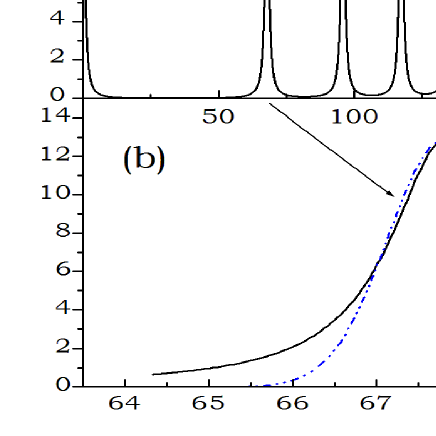
Figure 1: a) Positive energy branch of density of states obtained from the regularized GF for monolayer graphene at a magnetic field $B=10$ T. Positions of peaks are given by $E=\hbar\Omega\sqrt{n}$ with $\Omega=67.82$ meV and $n=0,\pm 1,\pm 2\ldots$. The broadening parameter is $\eta=1$ meV Jiang2007 ; Yang2010 . b) Detailed plot of DOS peak for the Landau level $n=1$. The difference between exact peak form and the Lorentz function is negligible within the plot accuracy. Dotted line: Gaussian like profile of the same FWHM.

In Fig. 1a we plot the unperturbed DOS as a function of energy in monolayer graphene calculated from the regular part of GF, see Eqs. (28) and (29), for $B=10$ T and $E\geq 0$. We assume a finite Landau level width $\eta=1$ meV, which agrees with experimental estimations of $\eta$ in graphene, see Refs. Jiang2007 ; Yang2010 . The DOS is a the series of nearly Lorentz-like peaks centered at $E_{n}=\hbar\Omega\sqrt{n}$, with $\Omega\simeq 67.82$ meV. For larger $n$, the peaks overlap with each other and DOS tends to a smooth function. In Fig. 1b we plot the DOS peak for Landau level $n=1$. We also plot the Gaussian-like peak having the same half-width. Differences between the Gaussian and the Lorentz functions exist in tails only, and they can be neglected for well-separated peaks.

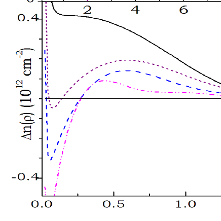
Figure 2: a) Position of the Fermi level for monolayer graphene in a magnetic field at constant electron density $n_{e}=0.35\times 10^{12}$ cm^-2 Ando2009 and broadening $\eta=1$ meV Jiang2007 ; Yang2010 . Vertical lines: magnetic fields used in lower panel. b) Radial parts of induced electron density $\Delta n({\bm{\rho}})$ in monolayer graphene around delta-like neutral impurity in a magnetic field. Parameter $V_{0}=-56$ eVŲ corresponds to nitrogen impurity Lambin2012 . Distance is given in magnetic length $L$ units.

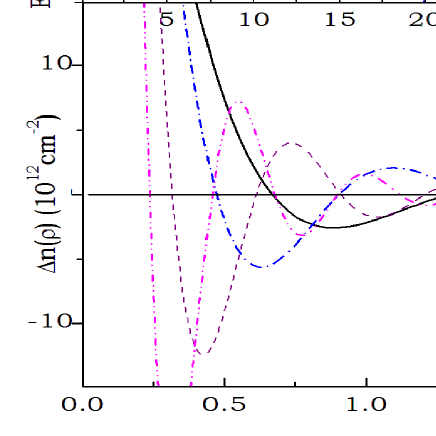
Figure 3: a) Position of the Fermi level for WS₂ in a magnetic field at constant electron density $n_{e}=5.9\times 10^{12}$ cm^-2 and broadening $\eta=0.74$ meV Wang2017 . $E_{F}$ is measured from the zero energy of the Hamiltonian (32), while the bottoms of conduction bands are at $E_{c}=\Delta/2=895$ meV. Vertical lines: magnetic fields used in lower panel. b) Radial parts of induced electron density $\Delta n({\bm{\rho}})$ in WS₂ around delta-like neutral impurity in a magnetic field. Parameter $V_{0}=-4.3$ eVŲ corresponds to nickel impurity in high-T_c superconductors Wang2005 . Distance is given in magnetic length $L$ units. Parabolic model of WS₂ bands is used.

As pointed out by Ando Ando2009 , the concentrations of electrons ($n_{e}>0$) and of the holes ($n_{e}<0$) in graphene can be controlled over a wide range of concentrations: $n_{e}\in[-5\times 10^{13}...5\times 10^{13}]$ cm^-2 by the gate voltage between graphene layer and heavily doped silicon. Below we take $n_{e}=0.35\times 10^{12}$ cm^-2, i.e. within the available range. In Fig. 2a we plot the Fermi level as a function of a magnetic field for monolayer graphene at $T=0$ for a fixed electron concentration $n_{e}$. The vertical lines indicate magnetic fields for which we calculate the oscillations of electron density. The Fermi level oscillates with a magnetic field, c.f. Ref. Zawadzki1984 . The oscillations occur when the electrons begin to fill the consecutive Landau level (LL), since the ’capacity’ of each LL increases with magnetic field. For sufficiently large fields all electrons are in the lowest LL with $n=0$, and the Fermi level drops to energies around zero.

In Fig. 2b we plot the induced electron density calculated from Eqs. (26) and (51) for a delta-like impurity placed at ${\bm{\rho}}_{0}={\bm{0}}$ for several values of magnetic field. We assume the impurity potential $V_{0}=-56$ eVŲ which corresponds to the nitrogen impurity in graphene in Ref. Lambin2012 , see Discussion. The calculations presented in Fig. 2b correspond to the standard experimental configuration in which a sample is placed in varying magnetic field. As seen in the figure, for all field values the induced density oscillates with the distance $r$ from the impurity, and the density oscillations are similar to FO in absence of fields. The periods of oscillations become longer with increasing field and the magnitudes of the oscillations increase. For all values of magnetic field the oscillations disappear for $r\geq 4L$. For $B=11$ T only one oscillation occurs, while for $B=2$ T the oscillations are irregular. To summarize, for typical material parameters of graphene and a nitrogen impurity it should be possible to observe FO in a magnetic field.

In Figs. 3a and 3b we present the results for WS₂. They are similar to those for monolayer graphene. The calculations are performed using the parabolic model of energy bands, see Eq. (47). The material parameters for WS₂ are listed in Table 1. Following experimental results of Ref. Wang2017 we take the electron density $n_{e}=5.9\times 10^{12}$ cm^-2 and broadening of LL equal to 2 meV of FWHM. This value corresponds to $\eta=0.74$ meV for the Lorentz peak given in Eq. (99) in Appendix C. Bottoms of the two conduction bands are located at $E_{c}=895$ meV, and the Fermi energy is counted from $E_{c}$. We take $V_{0}=-4.3$ eV$\AA^{2}$ which corresponds to nickel impurity in high-T_c superconductors Wang2005 , see Discussion.

The results in Fig. 3b are similar to these reported for graphene, but the oscillations are more pronounced. For all values of magnetic field one observes a few spatial oscillations vanishing for $r\geq 3L$. The oscillation periods increase with the field, but their amplitudes are less sensitive to field values. Since here $V_{0}<0$, the induced electron density increases in the vicinity of impurity because electrons are attracted by the well potential. Note that, for some $r$, the induced electron density $\Delta n({\bm{\rho}})$ may exceed the density of free electron gas $n_{e}=5.9\times 10^{12}$ cm^-2. This is an artifact of our model resulting from disregarding the many-body interactions in the electron gas, see Discussion.

In Figs. 2a and 3a the Fermi levels in the two samples exhibit saw-like oscillations with increasing magnetic field. To explain this behavior let us recall that the degeneracy of one LL is: $n_{LL}=eB/h\simeq 2.4\times$ 10${}^{10}\ B$ [cm^-2], where $B$ is measured in Tesla. For fixed electron density $n_{e}$, the increase of magnetic field results in pushing electrons towards lower Landau numbers $n$ Zawadzki1984 . Finally, for sufficiently high fields there is $n_{LL=0}>n_{e}$ and all electrons are at the lowest level. The oscillations in Figs. 2a and 3a are smoothed because of finite level widths $\Gamma$.

In two previous pictures we analyzed the FO in a wide scale of magnetic fields. Now we concentrate on FO in WS₂ for varying occupation of single Landau level close to $B=20$ T (see Fig. 3a), which corresponds to $n=3$. In Fig. 4 we calculate FO for five LL occupations and the offset we indicate magnetic fields corresponding to the five cases. General conclusion from Fig. 4 is that FO weakly depend on degree of occupation.

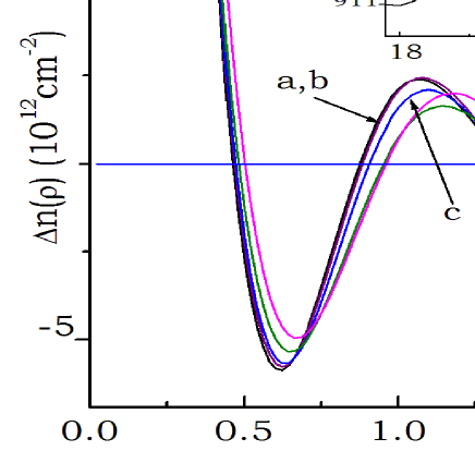
Figure 4: Radial parts of induced electron density $\Delta n({\bm{\rho}})$ in WS₂ around delta-like neutral impurity in a magnetic field. Model parameters are: $V_{0}=-4.3$ eVŲ and $\eta=0.74$ meV, see Fig. 3. Inset: The same as in Fig. 3a but for one peak of $E_{F}$ oscillations. Letters $a,b,c,d,e$ indicate magnetic fields used in the main figure.

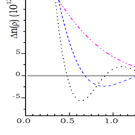
Figure 5: Radial parts of induced electron density $\Delta n({\bm{\rho}})$ in WS₂ around delta-like neutral impurity for a constant magnetic field $B=20$ T for various concentrations $n_{e}$ of electron gas. Model parameters are: $V_{0}=-4.3$ eVŲ and $\eta=0.74$ meV, see Fig. 3

In Fig. 5 we show results for several samples of different electron concentrations $n_{e}$ in the same magnetic field of $B=20$ T. For high $n_{e}$, the induced electron density oscillates, while for low $n_{e}$ the oscillations vanish. In all cases the oscillations disappear for $r\geq 3L$. For low $n_{e}$ the Fermi level is located in the lowest Landau level $n=0$ (in the so called quantum strong field limit) and the induced electron density decays exponentially with $r$ with a characteristic length on the order of $L$. Numerical fit in Fig. 5 to the curve for $n_{e}=10^{12}$ cm^-2 gives, to a high accuracy, the Gaussian form of the decay: $\Delta n({\bm{\rho}})\propto A\exp[-a(r-r_{0})^{2}]$, where $A,a,r_{0}>0$ are three positive constants. This result is similar to predictions for 3D electron gas and for delta-like and screened Coulomb-like impurities Rensink1968 ; Horing1969a .

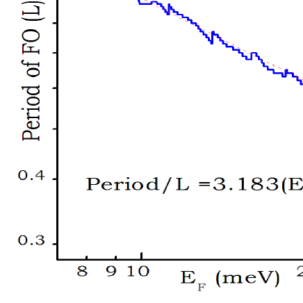
Figure 6: Period of Friedel oscillations vs. Fermi energy in WS₂ in a magnetic field $B=9$ T. Model parameters are: $V_{0}=-4.3$ eVŲ and $\eta=0.74$ meV, see Fig. 3.

In the field-free case FO arise from the sharp change of electron density in the $k$ space in the vicinity of the Fermi sphere, which leads to spatial oscillations of the density with the period $T_{FO}\propto\pi/k_{F}$, where $k_{F}$ is the Fermi vector. For free electrons in 2D there is $k_{F}\propto E_{F}^{1/2}$, which gives

$$T_{FO}\propto\frac{1}{\sqrt{E_{F}}}.$$ (55)

The main physical difference between 2D electrons in the presence or absence of a magnetic field is, that in the former case, the electron motion is fully quantized within the plane perpendicular to the field and for nonzero field there is no $k_{F}$ vector. However, since the Fermi energy is a well defined quantity both in the presence and absence of the field, we may expect that Eq. (55) remains valid also for the FO at nonzero magnetic field.

To verify this expectation, we plot in Fig. 6 the period of FO as a function of $E_{F}$ for $B=9$ T. As before, $E_{F}$ is measured from the conduction bands edges. The oscillation periods $T_{FO}$ are computed numerically as an average distance between several consecutive minima and maxima of induced electron density. The results are plotted in the logarithmic scale. As seen in Fig. 6, the periods $T_{FO}$ follow the formula of Eq. (55) to a high accuracy.

Equation (55) qualitatively explains the non-oscillating behavior of induced density in the quantum strong field limit. For group-VI dichalogenides, the lowest energy level in the conduction band is at $E=\Delta/2$ and in the quantum strong field limit there is $E_{F}=0$, since $E_{F}$ is measured from the bottom of conduction band, see Section II. Then the period of oscillations in Eq. (55) is infinite, which is equivalent to the non-oscillating decay of induced electron density.

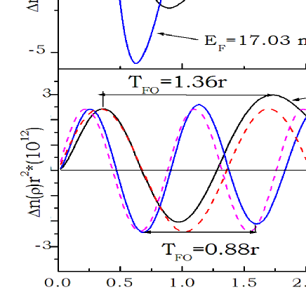
Figure 7: a) Radial parts of induced electron density $\Delta n({\bm{\rho}})$ in WS₂ around delta-like impurity for $n_{e}=5.9\times 10^{12}$ cm^-2 and $n_{e}=3.0\times 10^{12}$ cm^-2. The magnetic field is $B=20$ T. Fermi energies are located at $E_{F}=17.03$ meV and $E_{F}=7.02$ meV above the bottom of conduction band, respectively. Model parameters are: $V_{0}=-4.3$ eVŲ and $\eta=0.74$ meV, see Fig. 3. b) Solid lines: results from upper panel multiplied by $r^{2}$. Dotted lines: functions $\sin(2\pi r/T_{FO})$ for two $T_{FO}$ values.

As predicted by Rensink Rensink1968 and Horing Horing1969a , the FO in 3D should be expressed in terms of the sine or cosine functions of $(2k_{F}r)$ divided by $r^{-3}$, where $k_{F}$ is the Fermi vector. Having in mind this result and taking Eq. (55) we propose the following approximate formula for FO in the parabolic band model for electrons in group-VI dichalogenides

$$\Delta n({\bm{\rho}})\simeq\delta n\frac{\sin(2\pi r/T_{FO})}{r^{2}},$$ (56)

where $T_{FO}$ is given in Eq. (55) and $\delta n$ is a constant.

To verify the validity of Eq. (56), we plot in Fig. 7a the induced electron density $\Delta n({\bm{\rho}})$ in a magnetic field $B=20$ T for two values of electron concentration $n_{e}$ which correspond to two values of the Fermi energy. In Fig. 7b we isolate the oscillating part of the induced density: $\Delta n({\bm{\rho}})\times r^{2}$. It is seen that both solid curves oscillate with finite and nearly constant amplitudes. This leads to conclusion that, for large $r$, FO in a magnetic field decay as $r^{-2}$. This agrees with the field-free result in Eq. (1). As follows from Eq. (55), for a fixed magnetic field the product $T_{FO}\sqrt{E_{F}}$ is a constant, and this result is obtained for the two solid lines in Fig. 7b. Since the first oscillations of solid lines in Fig. 7b resemble the sines functions we plot in Fig. 7b two sine functions given by the numerator in Eq. (56), with the periods shown in the figure. For the first few cycles there is a good agreement between the exact results and the sine functions.

The results presented in Fig. 7b and in Eqs. (55) and (56) are extensions of the predictions of Refs. Rensink1968 ; Horing1969a concerning 2D electron gas in materials with honeycomb lattice. They are consistent with the perturbation approach, but our results are valid (within the validity of non-interacting gas model) for arbitrary electron concentrations, magnetic fields, impurity potentials $V_{0}$ and distances from the impurity, while the results of Refs. Rensink1968 ; Horing1969a have some limitations, see Discussion.

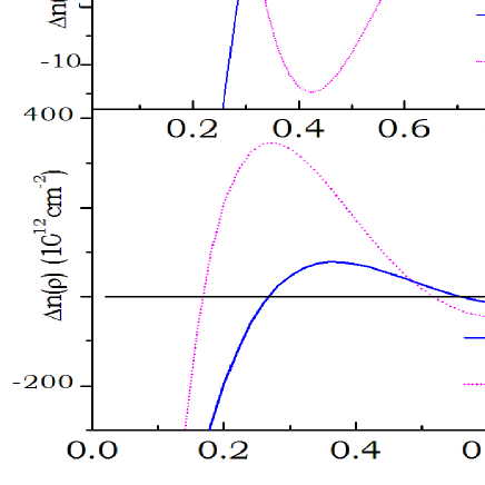
Figure 8: Radial part of induced electron density $\Delta n({\bm{\rho}})$ in WS₂ around delta-like neutral impurity in a magnetic field for attractive and repulsive $V_{0}$. a) For small $|V_{0}|$ values there is $\Delta n({\bm{\rho}})~{}\propto V_{0}$, see Eq. (57). b) For large $|V_{0}|$ values $\Delta n({\bm{\rho}})$ weakly depends on $V_{0}$, see Eq. (58).

In Fig. 8 we consider induced electron density $\Delta n({\bm{\rho}})$ for small and large values of $|V_{0}|$. For small $|V_{0}|$ one can neglect the denominators in Eq. (18) and obtain in the lowest order of the Born series

$$\hat{G}_{\bm{1},\bm{2}}\simeq\hat{g}_{\bm{1},\bm{2}}+\hat{g}_{\bm{1},\bm{0}}V_{r}\hat{g}_{\bm{0},\bm{2}}+\ldots.$$ (57)

Taking $V_{r}\simeq V_{0}$ we find that, for small $V_{0}$, there is $\Delta n({\bm{\rho}})\propto V_{0}$. To show this we plot $\Delta n({\bm{\rho}})$ for two opposite $V_{0}$ values and obtain two symmetric lines.

In Fig. 8b we plot $\Delta n({\bm{\rho}})$ for large $|V_{0}|$. In this case one can neglect the unity in the denominator of Eq. (18) which gives

$$\hat{G}_{\bm{1},\bm{2}}\simeq\hat{g}_{\bm{1},\bm{2}}+\hat{g}_{\bm{1},\bm{0}}\frac{1}{\hat{g}^{reg}}\hat{g}_{\bm{0},\bm{2}},$$ (58)

i.e. in this limit GF of the system and the resulting $\Delta n(\bm{\rho})$ do not depend on the impurity potential having an universal character.

IV Discussion

As shown in Figs. 6 and 7, equations (55) and (56) are valid for the ideal 2D electron gas and for that in group-VI dichalogenides in the parabolic approximation of energy band for typical material parameters. Our calculations for monolayer graphene and WS₂ in the nonparabolic bands model suggest that Eq. (56) should be replaced by

$$\Delta n({\bm{\rho}})\simeq\delta n\frac{F_{osc}[r,T_{osc}(r)]}{r^{2+\alpha}},$$ (59)

in which $0<\alpha<0.2$ and $F_{osc}$ is a bound and oscillating function of the distance. This results agrees with predictions for 2D massless Dirac fermions reported in Ref. Thakur2017 , where for large $\rho$ the authors predicted $\Delta n({\bm{\rho}})\propto\rho^{-3}$. In Eq. (59) the oscillation period $T_{osc}(r)$ increases with $r$ in a similar way to that shown in Fig. 7b. All quantities entering Eq. (59) depend on $V_{0}$. The numerical algorithms given in Appendix B allow one to calculate $\Delta n({\bm{\rho}})$ for various material parameters.

We considered a delta-like impurity potential of neutral impurity. With this choice it is possible to sum the Born series and obtain the exact GF. To estimate the range of validity of this model we first assume that a typical impurity size is on the order $r_{i}\approx 1-2$ Å, i.e. the size of an atom in the lattice. The impurity can be treated as delta-like if its size is much smaller than the oscillation period $T_{FO}$. As seen in Fig. 6, for a fixed magnetic field $T_{FO}$ decreases with the Fermi energy and electron concentration $n_{e}$. For parameters in Fig. 6 our model is valid for $T_{FO}\geq 20\AA$, i.e. for all $E_{F}$ values shown in the figure.

To consider the physical sense of approximating an impurity potential by the delta function we assume the potential to be short-range with a characteristic length $a$ centered at ${\bm{\rho}}=0$. Then the Dyson equation for GF is, see Eq. (8)

$$\hat{G}_{\bm{1},\bm{2}} = \hat{g}_{\bm{1},\bm{2}}+\int_{|\bm{\rho}|<a}\hat{g}_{\bm{1},\bm{3}}V({\bm{\rho}}_{3})\hat{G}_{\bm{3},\bm{2}}d^{2}{\bm{\rho}}_{3}$$ (60)

$$\simeq \hat{g}_{\bm{1},\bm{2}}+\hat{g}_{\bm{1},\bm{0}}V_{0}\hat{G}_{\bm{0},\bm{2}},$$ (61)

in which

$$V_{0}=\int_{|{\bm{\rho}}_{3}|<a}V({\bm{\rho}}_{3})d^{2}{\bm{\rho}}_{3}\simeq V(\bm{0})a^{2}\hskip 2.5pt{\rm[J\times m^{2}]}.$$ (62)

The model of a delta-like potential is valid if the integral in Eq. (60) is well approximated by Eqs. (61) and (62). In realistic systems the delta-like potential describes a potential of neutral impurity in the lattice, potential of a vacancy, contact potential arising from electron-nuclei interactions or potential of a screened ion having a short screening length. Equation (62) explains the physical units of $V_{0}$ entering into the Dyson equation, namely J$\times$m².

Now we discuss the magnitudes of $V_{0}$ used in the calculations is Section III. To select $V_{0}$ we take results reported in the literature concerning impurities, vacancies, dislocations or potential drops at surfaces. Wang et al. Wang2005 reported: $V_{0}=-4.3$ eV$\AA^{2}$ for nickel impurity, $V_{0}=11.2$ eV$\AA^{2}$ for zinc impurity and $V_{0}=69.3$ eV$\AA^{2}$ for a vacancy, respectively. These estimations are based on ab-initio calculations of Cu panels in high-T_c superconductors. Lang and Kohn calculated the effective one-electron potential for metal surface in the jellium model, (see Fig. 3 of Ref. Lang1970 or Fig. 2 of Ref. Dobson1995 ), which gives $V_{0}=16$ eVŲ.

Finally, one can estimate $V_{0}$ from impurity potentials used in ab-initio calculations. In Ref. Lambin2012 , the potential of nitrogen impurity in graphene was assumed in the Gaussian form

$$V(\bm{\rho})=\epsilon_{C}-4.0\exp\left(-\frac{\rho^{2}}{2\sigma^{2}}\right)\hskip 5.0pt{\rm[eV]},$$ (63)

where $\epsilon_{C}$ is the asymptotic bulk value of the on-site parameter of carbon, and $\sigma=1.5$ Å. Performing integration in Eq. (62) for potential in Eq. (63) we find: $V_{0}=-2\pi\times 4.0\times\sigma^{2}=-56$ eVŲ.

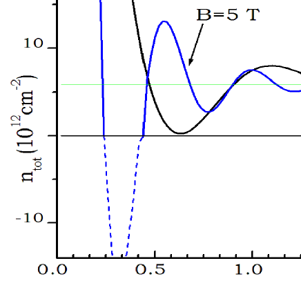
Figure 9: Radial parts of total electron density $n_{tot}=n_{e}+\Delta n(\bm{\rho})$ calculated for WS₂ around delta-like neutral impurity in a magnetic field. Dotted line indicates schematically non-physical negative total electron density.

As seen in Fig. 2, for monolayer graphene the induced electron density does not exceed the background density $n_{e}=0.35\times 10^{12}$ cm^-2, so that the total density of electron gas: $n_{tot}=n_{e}+\Delta n(\bm{\rho})>0$ for all ${\bm{\rho}}$. However, in WS₂, for small $r$ and low magnetic fields the magnitude of $\Delta n(\bm{\rho})$ exceeds the electron density $n_{e}=5.9\times 10^{12}$ cm^-2. Thus, for some $r$, there is $n_{tot}<0$, which is an artifact of the model.

To analyze this question we note first that the calculations in Section II are exact in the sense that we sum the perturbation series in Eq. (10) to the infinite order, so that our results are valid for arbitrary $V_{0}$ and $E$ values. However, there remain limitations of the free-electron model. To estimate the validity of the free-electron approximation, we plot schematically in Fig. 9 the total electron density with an additional condition $n_{tot}\geq 0$. The dotted line indicates the non-physical case of negative $n_{tot}$. It is seen that, for $B=20$ T, for all $r$ there is $n_{tot}>0$, and the model of noninteracting electron gas used above is correct. Similarly, for $B=5$ T there is $n_{tot}>0$ for $r>0.5L$, which determines the range of validity of the model. The conclusion from Fig. 9 is that the model of non-interacting electrons applied to the calculation of FO in a magnetic field for electrons in 2D materials with a honeycomb lattice is valid under certain conditions. First, the impurity potential $V_{0}$ should be weak and possibly attractive ($V_{0}<0$). Next, both the magnetic field and electron density $n_{e}$ should be high. Finally, in some cases the results for small $r$ may be doubtful, but they become reasonable for large distances from the impurity.

In the literature describing the electron gas in metals there exist quantities obtained by the theory of non-interacting particles which are unphysical while those obtained within the many-body theories do not suffer from this deficiency. For example the so-called pair distribution function $g(r)$, describing the probability of finding an electron in a distance $r$ from the impurity, should be strictly positive. However, as pointed out in Ref. Sjolander1972 , the calculations of $g(r)$ within linear model lead for some $r$ to negative values of $g(r)$. On the other hand, by including electron-electron interactions, exchange and non-linear effects one obtains positive values of $g(r)$ for all distances, see Refs. Perdew1992 ; Vericat2011 . For this reason we expect that the account of the electron-electron interaction would correct the nonphysical effects for FO oscillations at small distances from the impurity.

Let us now turn to the regularization procedure and the divergences in $\hat{g}_{\bm{0},\bm{0}}$. The origin of these divergencies arises from the divergences of harmonic series in Eq. (11) for large $n$, i.e. for large energies. However, the $\bm{k}\cdot\bm{p}$ model is valid for energies near band extrema, i.e. for small $n$. The divergences appearing in Eq. (11) are artifacts of the model which justifies the use of regularization procedure described in Section II.

As mentioned in Introduction, the regularization procedure is based on two elements. First, for all models in Section II there exist analytical expressions for sums over Laguerre polynomials see Eq. (7). Second, knowing the limit of the Whittaker function for small arguments one can isolate the divergent and regular parts of GF, see Eqs. (13)–(16). If one were unable to sum up an infinite series in Eq. (5), one would be unable to isolate divergent and regular parts of $\hat{g}$. Therefore, the knowledge of analytical form of the one-electron GF is necessary to perform the regularization procedure described in Section II.

There exists another consequence of the divergencies in $\hat{g}_{\bm{0},\bm{0}}$ of Eq. (10), namely the impossibility of the perturbation expansion of the Dyson equation into the Born-von Neumann series. Treating, incorrectly, $V_{0}\hat{g}_{\bm{0},\bm{0}}$ as an expansion parameter, one obtains

$$\hat{G}_{\bm{1},\bm{2}}\simeq\hat{g}_{\bm{1},\bm{2}}+\hat{g}_{\bm{1},\bm{0}}V_{0}\hat{g}_{\bm{0},\bm{2}}+\hat{g}_{\bm{1},\bm{0}}\left[V_{0}\hat{g}_{\bm{0},\bm{0}}V_{0}\right]\hat{g}_{\bm{0},\bm{2}}+\ldots.$$

In the above series the first and second terms are finite, but the remaining terms diverge because they include the powers of $\hat{g}_{\bm{0},\bm{0}}$. There is no rigorous method of removing these divergencies from the above series. The correct way of obtaining the perturbation series of Born-von Neumann is the use of Eq. (18) instead Eq. (10):

$$\hat{G}_{\bm{1},\bm{2}}\simeq\hat{g}_{\bm{1},\bm{2}}+\hat{g}_{\bm{1},\bm{0}}V_{r}\hat{g}_{\bm{0},\bm{2}}+\hat{g}_{\bm{1},\bm{0}}\left[V_{r}\hat{g}_{\bm{0},\bm{0}}^{reg}V_{r}\right]\hat{g}_{\bm{0},\bm{2}}+\ldots,$$ (64)

where $V_{r}$ is defined in Eq. (19). The above expansion holds for $y=V_{r}\hat{g}_{\bm{0},\bm{0}}\ll 1$.

In Eq. (19) we defined the regularized potential $V_{r}$ and claimed that, in practice, there is $V_{r}\simeq V_{0}$. Now we discuss validity of this assumption. Let us consider monolayer graphene for $B=10$ T. In Eq. (26) we take: $\hbar\Omega=67.8$ meV, $L=81.1$ Å and $V_{0}=-56$ eVŲ. For $\zeta=2.7$ Å, i.e. for the size of a neutral atom in the lattice we obtain from Eq. (19): $|V_{0}\hat{g}_{\bm{0},\bm{0}}|=0.04$, and one can approximate $V_{r}\simeq V_{0}$. For $\zeta=5$ fm, i.e. the size of a typical atomic nuclei, one obtains: $|V_{0}\hat{g}_{\bm{0},\bm{0}}|=0.39$, which gives $V_{r}=1.64V_{0}$ for negative $V_{0}$ and $V_{r}=0.72V_{0}$ for positive $V_{0}$. Then there is $V_{r}=cV_{0}$ where $c$ is still on the order of unity. The potential of atomic nuclei is the narrowest realistic potential appearing in the solid state materials, so that the regularization procedure in Section II leads to reasonable results.

There exist several other approaches allowing one to overcome the problem of divergence of $\hat{g}_{\bm{0},\bm{0}}$ in Eq. (10). First, one can truncate the harmonic series in Eq. (11) at certain $n_{max}$, e.g. for energies $\hbar\Omega n_{max}$ exceeding the electron energies in the first BZ. Second, one can add a convergence factor to the series in Eq. (11), allowing one to sum up the series. Finally, one can replace the ${\bm{k}}\cdot{\bm{p}}$ Hamiltonian by the more accurate tight-binding model, which automatically introduces a cut-off in the energy scale. Each of the above methods handles the problem of divergence, but it introduces either an artificial cut-off or convergence factors, or leads to a non-analytical form of the one-electron GF. The regularization procedure described in Section II is not better than the discussed alternatives, but is more elegant and rigorous.

In our approach we assume low concentrations of neutral impurities. This assumption is valid when the average distance $R_{NN}$ between nearest-neighbor impurities exceeds the range of density oscillations. As seen in Figs. 2 and 3, there is $R_{NN}>3L$, depending on the strength of a magnetic field, which gives $R_{NN}>200$ Å. This corresponds to impurity concentrations $n_{i}<0.25\times 10^{12}$ cm^-2. For higher $n_{i}$, the densities induced by the two neighboring impurities overlap with each other and the correlations effects between the two impurities should be taken into account.

As mentioned above, position of the Fermi level is calculated for impurity-free electron gas. This approach is common in the literature, but it neglects the change of $E_{F}$ due to presence of impurities. The argument supporting this approach is that for low impurity concentration the change of the electron gas density is spatial but not total.

Calculations of FO for 2D massive Dirac fermions in absence of magnetic field using dielectric function approach were carried out by Thakur2017 . As to the Dirac fermions in a magnetic field, in Ref. Yuan2012 the authors calculated the polarization function for graphene in strong fields, but they did not consider the density oscillations.

In our calculations we assumed $T=0$ limit. The results can be generalized in the standard way to finite temperatures by i) replacing the zero-temperature Green’s functions $\hat{g}(E)$ by $\hat{g}(i\hbar\omega_{m})$, where $\omega_{m}=(2\pi+1)k_{B}T/\hbar$ and $m$ is an integer, ii) replacing in Eq. (50) the integration over the energy by the summation over $m$, iii) adding the Fermi-Dirac distribution function to the integral in Eq. (50). For finite $T$ in absence of fields the electron distribution is spread over a wider energy range than for $T=0$ and there is a wider range of ${\bm{k}}$ vectors allowed for the redistribution. As a result, for $T>0$ FO have the same period as for $T=0$, but there appear additional temperature-depending damping factors, see Ref. Grassme1993 . Similar effects are expected for FO in 2D electron gas in a magnetic field.

In the integral in Eq. (50) we introduced the cut-off energy in the lower limit which, in our calculations, is a few meV below the bottoms of the conduction bands. We do not integrate over the filled valence bands since they do not give contributions to the oscillating induced density. However, we performed calculations treating the cut-off energy $E_{x}$ as a variable parameter. No significant change of the results occurred, but there appeared oscillations having small amplitude and frequency $\omega_{x}=E_{x}/\hbar$. To eliminate these artifacts, one should take $E_{x}$ sufficiently deep in the valence bands.

Promising experimental methods for observation of FO in 2D materials with honeycomb lattice are the scanning tunneling spectroscopy and the scanning tunneling microscopy, both successfully used for observation of the FO in absence of fields Kanisawa2001 ; Hasegawa2007 ; Sessi2015 . In these experiments, usually performed at low temperatures, the modulation of the local density of states can be resolved by differential conductivity maps ($dI/dU$). Recently, similar measurements were performed by Misra et al. with the scanning tunneling microscope at high magnetic field Misra2013 . This method seems to be appropriate for experimental observation of FO in a magnetic field for 2D electron gases.

V Summary

The Friedel density oscillations induced by a delta-like neutral impurity in 2D electron gases in the presence of a magnetic field are calculated. Exact renormalized Green’s functions obtained by an exact summation of the corresponding Dyson series are used in the calculations. The renormalization procedures are first demonstrated using the simple case of free 2D electron gas and then the developed methods are used to treat the realistic cases of monolayer graphene and group-VI dicalchogenides employing the appropriate band structures of these materials. Final results for FO are presented which are valid for wide ranges of impurity potential strengths, electron densities, magnetic fields and distances from impurity. Realistic models of neutral impurities in the materials of interest are employed. It is found that, for weak impurity potentials, the FO amplitudes are proportional to the potential strength. The obtained formulas for FO are discussed and compared to results for 3D electron gases in a magnetic field. In particular, it is shown that the Fermi vector in a 3D electron gas is replaced by a corresponding quantity for a 2D gas calculated from the Fermi energy. In some particular situations: low magnetic fields, repulsive impurity potential and small distances from impurity, the total calculated electron density becomes negative. which indicates limitations of the one-body theory.

Appendix A Green’s function in group-VI dichalcogenides

We present here details of calculations of the one-electron Green’s function for electrons in group-VI dichalcogenides in the presence of a magnetic field. At the ${\bm{K}}$ point of BZ the eigenstates of the Hamiltonian (32) for $n\geq 1$ are

$$\Psi_{nk_{x}+}({\bm{\rho}}) = \frac{e^{ik_{x}x}}{\sqrt{2\pi}{\cal N}_{n}}\left(\begin{array}[]{c}-\hbar\Omega\sqrt{n}\phi_{n-1}(\xi)\\ (E_{n}-E_{w})\phi_{n}(\xi)\end{array}\right),$$ (67)

$$\Psi_{nk_{x}-}({\bm{\rho}}) = \frac{e^{ik_{x}x}}{\sqrt{2\pi}{\cal N}_{n}}\left(\begin{array}[]{c}(E_{n}-E_{w})\phi_{n-1}(\xi)\\ \hbar\Omega\sqrt{n}\phi_{n}(\xi)\end{array}\right),$$ (70)

and the eigenenergies $E_{nk_{x}\epsilon}$ are given in Eq. (33). There is ${\cal N}_{n}=\sqrt{2E_{n}(E_{n}-E_{w})}$, where $E_{w}$ and $E_{n}$ are defined in Eqs. (31) and (33), respectively. For $n=0$ there is

$$\Psi_{0k_{x}+}({\bm{\rho}}) = 0$$ (71)

$$\Psi_{0k_{x}-}({\bm{\rho}}) = \frac{e^{ik_{x}x}}{\sqrt{2\pi}}\left(\begin{array}[]{c}0\\ \phi_{0}(\xi)\end{array}\right),$$ (74)

and the eigenenergy is $E_{0k_{x},-1,s_{z}}=-E_{w}+E_{s_{z}}$. For further calculations it is convenient to introduce the notation: $\Psi_{nk_{x}+}=(\psi_{+}^{u},\psi_{+}^{l})^{\dagger}$ and $\Psi_{nk_{x}-}=(\psi_{-}^{u},\psi_{-}^{l})^{\dagger}$.

Consider the Hamiltonian (32) with the eigenvalues given in Eq. (33) and eigenvectors in Eqs. (67)–(70). For $\tau=+1$ and both $s_{z}$ orientations the stationary GF of the Hamiltonian (32) is

$$\hat{g}_{+}({\bm{\rho}},{\bm{\rho}}^{\prime},{\cal Z})=\left(\begin{array}[]{cc}\hat{\gamma}^{uu}_{+}&\hat{\gamma}^{ul}_{+}\\ \hat{\gamma}^{lu}_{+}&\hat{\gamma}^{ll}_{+}\end{array}\right)+\left(\begin{array}[]{cc}0&0\\ 0&{\cal C}_{+}\end{array}\right)\equiv\left(\begin{array}[]{cc}\hat{g}^{uu}_{+}&\hat{g}^{ul}_{+}\\ \hat{g}^{lu}_{+}&\hat{g}^{ll}_{+}\end{array}\right),$$ (75)

where

$$\left(\begin{array}[]{cc}\hat{\gamma}^{uu}_{+}&\hat{\gamma}^{ul}_{+}\\ \hat{\gamma}^{lu}_{+}&\hat{\gamma}^{ll}_{+}\end{array}\right)=\sum_{n>0,k_{x},\epsilon}\frac{\psi_{nk_{x}\epsilon}\psi_{nk_{x}\epsilon}^{\dagger}}{{\cal Z}-E_{nk_{x}\epsilon}}$$ (76)

and

$$\left(\begin{array}[]{cc}0&0\\ 0&{\cal C}_{+}\end{array}\right)=\sum_{k_{x},\epsilon}\frac{\psi_{0k_{x}\epsilon}\psi_{0k_{x}\epsilon}^{\dagger}}{{\cal Z}-E_{0k_{x}\epsilon}}\delta_{\epsilon,-1}.$$ (77)

For $\hat{\gamma}^{uu}_{+}({\cal Z})$ the summation over $\epsilon=\pm 1$ gives

$$\hat{\gamma}^{uu}_{+}({\cal Z})=-\sum_{n>0,k_{x}}\left(\frac{\psi_{+}^{u}\psi_{+}^{u*}}{{\cal Z}_{+}-E_{n}}+\frac{\psi_{-}^{u}\psi_{-}^{u*}}{{\cal Z}_{+}+E_{n}}\right),$$ (78)

in which ${\cal Z}_{+}={\cal Z}-E_{s_{z}}$, and $\psi_{\pm}^{u}$ are defined in Eqs. (67) and (70). For $\hat{\gamma}^{ul}_{+}$, $\hat{\gamma}^{lu}_{+}$, $\hat{\gamma}^{ll}_{+}$, ${\cal C}_{+}$ the summation over $\epsilon=\pm 1$ is performed similarly. Calculating in Eq. (78) the integral over $k_{x}$ we use the identity, (see formula 7.377 in GradshteinBook )

$$\int_{-\infty}^{\infty}\!\!\!\!e^{-x^{2}}{\rm H}_{m}(x+y){\rm H}_{n}(x+z)dx=2^{n}\sqrt{\pi}m!z^{n^{\prime}}{\rm L}_{m}^{n^{\prime}}(-2yz),$$ (79)

where $n^{\prime}=n-m$, $m\leq n$, and $L_{n}^{\alpha}(t)$ are the associated Laguerre polynomials. One gets

$$\hat{\gamma}^{uu}_{+}({\bm{\rho}},{\bm{\rho}}^{\prime},{\cal Z}) = -(\bar{\cal Z}+\bar{E}_{w})\sum_{n=1}^{\infty}\frac{A(\Omega)L_{n-1}^{0}(r^{2})}{n+\bar{E}_{w}^{2}-\bar{\cal Z}^{2}},$$ (80)

$$\hat{\gamma}^{ll}_{+}({\bm{\rho}},{\bm{\rho}}^{\prime},{\cal Z}) = -(\bar{\cal Z}-\bar{E}_{w})\sum_{n=1}^{\infty}\frac{A(\Omega)L_{n}^{0}(r^{2})}{n+\bar{E}_{w}^{2}-\bar{\cal Z}^{2}},$$ (81)

$${\cal C}_{+}({\bm{\rho}},{\bm{\rho}}^{\prime},{\cal Z}) = -(\bar{\cal Z}-\bar{E}_{w})\frac{A(\Omega)L_{0}^{0}(r^{2})}{\bar{E}_{w}^{2}-\bar{\cal Z}^{2}},$$ (82)

$$\hat{\gamma}^{ul}_{+}({\bm{\rho}},{\bm{\rho}}^{\prime},{\cal Z}) = m_{cd}\sum_{n=1}^{\infty}\frac{A(\Omega)L_{n-1}^{1}(r^{2})}{n+\bar{E}_{w}^{2}-\bar{\cal Z}^{2}},$$ (83)

where $\bar{\cal Z}={\cal Z}_{+}/(\hbar\Omega)$, $\bar{E}_{w}=E_{w}/(\hbar\Omega)$, $r^{2}=({\bm{\rho}}-{\bm{\rho}}^{\prime})^{2}/(2L^{2})$ and $A(\Omega)$ is defined in Eq. (6). In Eq. (83) we defined $m_{ul}=[(y-y^{\prime})+i(x-x^{\prime})]/(\sqrt{2}L)$. For $\hat{\gamma}^{lu}_{+}$ one obtains expression analogous to that for $\hat{\gamma}^{ul}_{+}$, but with $m_{ul}$ replaced by $m_{lu}=[(y^{\prime}-y)+i(x-x^{\prime})]/(L\sqrt{2})$.

In Eqs. (80)–(81) the summation over Landau levels $n$ is performed with the use of formulas 6.12.4 and 6.9.4 in ErdelyiBook

$$t^{-\beta}\sum_{n=0}^{\infty}\frac{L_{n}^{-\beta}(t)}{n+a-\beta}=\Gamma(a-\beta)\Psi(a,\beta+1;t)$$

$$=\Gamma(a-\beta)e^{t/2}t^{-1/2-\beta/2}W_{\beta/2+1/2-a,\beta/2}(t),$$ (84)

where $\Psi(a,c;t)$ is the second solution of the confluent hypergeometric equation ErdelyiBook , and $W_{\kappa,\mu}(t)$ is the Whittaker function. The series in Eq. (84) converges for $t>0$ and $\beta>-1/2$. When combining Eqs. (80)–(84) we set $t=r^{2}$ and, for $\hat{\gamma}^{uu}_{+}$ and $\hat{\gamma}^{ll}_{+}$ we take $\beta=0$. To calculate $\hat{\gamma}^{uu}_{+}$ in Eq. (80) we first change the summation index $n^{\prime}=n-1$, and then set $a=1+\bar{E}_{w}^{2}-\bar{\cal Z}^{2}$ in Eq. (84). Similarly, calculating the sum $\hat{\gamma}^{ll}_{+}+{\cal C}_{+}$ we set $a=\bar{E}_{w}^{2}-\bar{\cal Z}^{2}$. Then we find

$$\hat{g}^{uu}_{+}\equiv\hat{\gamma}^{uu}_{+} = -\frac{(\bar{\cal Z}+\bar{E}_{w})e^{i\chi}}{2\pi\hbar\Omega L^{2}|r|}{\cal W}_{\kappa_{u}}(r^{2}),\$$ (85)

$$\hat{g}^{ll}_{+}\equiv\hat{\gamma}^{ll}_{+}+{\cal C}_{+} = -\frac{(\bar{\cal Z}-\bar{E}_{w})e^{i\chi}}{2\pi\hbar\Omega L^{2}|r|}{\cal W}_{\kappa_{l}}(r^{2}),$$ (86)

where $\kappa_{u}=\bar{\cal Z}^{2}-\bar{E}_{w}^{2}-1/2$, $\kappa_{l}=\bar{\cal Z}^{2}-\bar{E}_{w}^{2}+1/2$, and ${\cal W}_{\kappa}(z)=\Gamma(1/2-\kappa)W_{\kappa,0}(z)$. For $\hat{\gamma}^{ul}_{+}$ there is $\beta=-1$ in Eq. (84), which is beyond the convergence range of the series. However, $\hat{\gamma}^{ul}_{+}$ can be expressed as a combination of $\hat{\gamma}^{uu}_{+}$ and $\hat{\gamma}^{ll}_{+}$ functions by using the identity $L_{n-1}^{1}(r^{2})=n[(L_{n-1}^{0}(r^{2})-L_{n}^{0}(r^{2})]/r^{2}$, see formula 8.971.4 in GradshteinBook . Then we obtain

$$\hat{g}^{ul}_{+}\equiv\hat{\gamma}^{ul}_{+}=\frac{m_{ul}}{r^{2}}\left[(\bar{\cal Z}-\bar{E}_{w})\hat{g}^{uu}_{+}-(\bar{\cal Z}+\bar{E}_{w})\hat{g}^{ll}_{+}\right],$$ (87)

where $m_{ul}$ is defined in Eq. (83). Since GF is a hermitian operator, there is $\hat{g}_{+}({\bm{\rho}},{\bm{\rho}}^{\prime},E)=\langle{\bm{\rho}}|(E-\hat{H})^{-1}|{\bm{\rho}}^{\prime}\rangle=\hat{g}_{+}({\bm{\rho}}^{\prime},{\bm{\rho}},E)^{\dagger}$. By interchanging ${\bm{\rho}}$ with ${\bm{\rho}}^{\prime}$ in Eqs. (85)–(87) one finds: $\hat{g}^{cc}_{+}({\bm{\rho}},{\bm{\rho}}^{\prime})=\hat{g}^{cc}_{+}({\bm{\rho}}^{\prime},{\bm{\rho}})^{*}$ with $c\in\{u,l\}$, and $\hat{g}^{ul}_{+}({\bm{\rho}},{\bm{\rho}}^{\prime})=\hat{g}^{lu}_{+}({\bm{\rho}}^{\prime},{\bm{\rho}})^{*}$. This verifies the hermiticity of GF in Eqs. (85)–(87).

Now we show that, for ${\bm{\rho}}\rightarrow{\bm{\rho}}^{\prime}$, there is $\hat{g}^{ul}_{+}({\bm{\rho}},{\bm{\rho}},{\cal Z})=\hat{g}^{ul}_{{\bm{0}},{\bm{0}},+}=0$. To prove this we turn to Eq. (75) and after short algebra we find

$$\hat{g}^{ul}_{+}({\bm{\rho}},{\bm{\rho}}^{\prime},{\cal Z})=-\frac{\hbar\Omega}{2\pi}\sum_{n}\!\int_{-\infty}^{\infty}\!\!\frac{\sqrt{n}e^{ik_{x}(x-x^{\prime})}\phi_{m}(\xi)\phi_{n}(\xi^{\prime})^{*}}{\hbar^{2}\Omega^{2}n+E_{w}^{2}-{\cal Z}^{2}}dk_{x},$$ (88)

with $m=n-1$. Taking the limit ${\bm{\rho}}\rightarrow{\bm{\rho}}^{\prime}$ we have $x=x^{\prime}$ and $\xi=\xi^{\prime}$. Then using $d\xi=-Ldk_{x}$ we obtain

$$\hat{g}^{ul}_{+}({\bm{\rho}},{\bm{\rho}},{\cal Z})=\frac{\hbar\Omega}{2\pi L}\sum_{n}\!\int_{-\infty}^{\infty}\!\!\frac{\sqrt{n}\phi_{m}(\xi)\phi_{n}(\xi)}{\hbar^{2}\Omega^{2}n+E_{w}^{2}-{\cal Z}^{2}}d\xi=0,$$ (89)

because of the orthogonality of the Hermite functions $\phi_{m}(\xi)$ and $\phi_{n}(\xi)$ for $n\neq m$. For the same reason there is  $\hat{g}^{lu}_{+}({\bm{\rho}},{\bm{\rho}},{\cal Z})=0$. Since $\hat{g}^{ul}_{+}({\bm{\rho}},{\bm{\rho}},{\cal Z})$ and $\hat{g}^{lu}_{+}({\bm{\rho}},{\bm{\rho}},{\cal Z})$ vanish, there is also $\hat{g}_{ul+}^{reg}=0$, $\hat{g}_{ul+}^{div}=0$, $\hat{g}_{lu}^{reg+}=0$ and $\hat{g}_{lu+}^{div}=0$, see Eqs. (27)–(29) and (42)–(45).

For the ${\bm{K}^{\prime}}$ point of BZ, the Hamiltonian $\hat{H}^{\prime}$ is given in Eq. (34). The stationary GF of the Hamiltonian $\hat{H}^{\prime}$ is $\left(\begin{array}[]{cc}\hat{g}^{uu}_{-}&\hat{g}^{ul}_{-}\\ \hat{g}^{lu}_{-}&\hat{g}^{ll}_{-}\end{array}\right)$, see Eq. (75). Proceeding similarly as for the ${\bm{K}}$ point we find

$$\hat{g}^{uu}_{-} = -\frac{(\bar{\cal Z}^{\prime}+\bar{E}_{w})e^{i\chi}}{2\pi\hbar\Omega L^{2}|r|}{\cal W}_{\kappa_{u}^{\prime}}(r^{2}),\$$ (90)

$$\hat{g}^{ll}_{-} = -\frac{(\bar{\cal Z}^{\prime}-\bar{E}_{w})e^{i\chi}}{2\pi\hbar\Omega L^{2}|r|}{\cal W}_{\kappa_{l}^{\prime}}(r^{2}),$$ (91)

$$\hat{g}^{ul}_{-} = \frac{m_{ul}}{r^{2}}\left[(\bar{\cal Z}^{\prime}-\bar{E}_{w})\hat{g}^{ll}_{-}-(\bar{\cal Z}^{\prime}+\bar{E}_{w})\hat{g}^{uu}_{-}\right],$$ (92)

where $\kappa_{u}^{\prime}=\bar{\cal Z}^{{}^{\prime}2}-\bar{E}_{w}^{{}^{\prime}2}+1/2$, $\kappa_{l}^{\prime}=\bar{\cal Z}^{{}^{\prime}2}-\bar{E}_{w}^{{}^{\prime}2}-1/2$, and ${\cal W}_{\kappa}(z)=\Gamma(1/2-\kappa)W_{\kappa,0}(z)$ with ${\cal Z}^{\prime}={\cal Z}-E_{s_{z}}^{\prime}$. The total GF is a $8\times 8$ block-diagonal matrix consisting of four $2\times 2$ blocks given in Eqs. (75) and (92) with four combinations of $\tau=\pm 1$ and $s_{z}\pm 1$ quantum numbers.

Appendix B Numerical calculations of Whittaker functions

One of the crucial elements in the calculations of Section III is to use a fast and accurate numerical procedure to obtain the Whittaker functions $W_{\kappa,0}(z)$ and ${\cal W}_{\kappa}(z)$ appearing in the final formulas for the one-electron GF, see Eq. (7). In this Appendix we collect numerical algorithms for calculating $W_{\kappa,0}(z)$ for various ranges of $\kappa$ and $z$.

It is useful to express GF in terms of the Whittaker functions $W_{\kappa,0}(z)$, as given in Eq. (7), because $W_{\kappa,0}(z)$ can be conveniently computed from the formula 9.237.1 in Ref. GradshteinBook :

$$W_{\kappa,0}(z) = \frac{\sqrt{z}\ e^{-z/2}}{\Gamma(1/2-\kappa)^{2}}\sum_{k=0}^{\infty}\frac{\Gamma(k-\kappa+1/2)}{(k!)^{2}}z^{k}\times$$ (93)

$$\left[2\psi(k+1)-\psi(k-\kappa+1/2)-\ln(z)\right],$$

where $\psi(z)=d\ln[\Gamma(z)]/dz$ and $|{\rm arg}(z)|<3\pi/2$. In practical calculations it is helpful to calculate the function: ${\cal W}_{\kappa}(z)=\Gamma(1/2-\kappa)W_{\kappa,0}(z)$. In this case, applying $k$ times the identity: $\Gamma(1/2-\kappa+k)=(1/2-\kappa+k-1)\Gamma(1/2-\kappa+k-1)$, one avoids the direct calculation of $\Gamma(1/2-\kappa)$ function, which simplifies calculations of ${\cal W}_{\kappa}(z)$ for large $\kappa$. This method gives stable numerical results within the rectangular: $-5<{\rm Re}(\kappa)<25$ and $0<z<25$. For ${\rm Re}(\kappa)$ outside the above region, the formula in Eq. (93) gives erroneous results due to truncation errors. To avoid these problems, we devised a numerically-stable iterative algorithm of calculating the Whittaker function for large values of ${\rm Re}(\kappa)$.

Consider the identity 13.4.31 in Ref. AbramowitzBook for $W_{\kappa,0}(z)$

$$W_{\kappa+1,0}(z)=-(2\kappa-z)W_{\kappa,0}(z)-(\kappa-1/2)^{2}W_{\kappa-1,0}(z).$$ (94)

On multiplying both sides by $\Gamma(1/2-\kappa-1)(-1)^{{\rm Re}(\kappa)+1}$ and using three times the identity $\Gamma(x+1)=x\Gamma(x)$ one obtains

$${\cal W}_{\kappa+1}^{-}(z)=-\frac{2\kappa-z}{\kappa+1/2}{\cal W}_{\kappa}^{-}(z)-\frac{\kappa-1/2}{\kappa+1/2}{\cal W}_{\kappa-1}^{-}(z),$$ (95)

where ${\cal W}_{\kappa}^{-}(z)={\cal W}_{\kappa}(z)(-1)^{{\rm Re}(\kappa)}$. Equation (95) allows one to calculate iteratively ${\cal W}_{\kappa}^{-}(z)$ for $z>0$ and large ${\rm Re}(\kappa)>0$ values. To show the stability of the iterative scheme in Eq. (95) we consider the limit of both sides of Eq. (95) for large $\kappa$ values

$${\cal W}_{\kappa+1}^{-}(z)\simeq\left(2-\frac{z}{\kappa}\right){\cal W}_{\kappa}^{-}(z)-{\cal W}_{\kappa-1}^{-}(z).$$ (96)

Consider now a function $f(\kappa)$ satisfying the second-order differential equation: $f^{"}(\kappa)=-\omega^{2}f(\kappa)$. Then $f(\kappa)=C\sin(\omega\kappa+\phi)$, where the constants $C$ and $\phi$ are determined from the initial conditions. Approximating the second derivative $f^{"}(\kappa)$ by a finite difference one obtains

$$f_{\kappa+1}=(2-\omega^{2}h^{2})f_{\kappa}-f_{\kappa-1}.$$ (97)

The iteration scheme in Eq. (97) is numerically stable for $(\omega^{2}h^{2})<1$, which may be verified by direct calculations.

By comparing Eq. (97) with Eq. (96), taking $h=1$ and $\omega=\sqrt{z/\kappa}$ we find that i) for large ${\rm Re}(\kappa)$ the iteration scheme in Eq. (96) is numerically stable for $(z/\kappa)<1$, and ii) for large $\kappa$ values there is: ${\cal W}_{\kappa+1}^{-}(z)\simeq A\sin(\sqrt{z\kappa}+\Phi)$, i.e. ${\cal W}_{\kappa}^{-}(z)$ oscillates with a finite amplitude.

The factor $(-1)^{{\rm Re}(\kappa)}$ in definition of ${\cal W}_{\kappa}^{-}(z)$ plays the key role in the iteration scheme in Eq. (96), since it ensures the negative sign in front of $(z/\kappa)$ term. If one iterated ${\cal W}_{\kappa}(z)$ instead of ${\cal W}_{\kappa}^{-}(z)$ and the factor $(-1)^{{\rm Re}(\kappa)}$ were omitted, the corresponding sign in front of $(z/\kappa)$ term in Eq. (96) would be positive and the iterating scheme would diverge.

The iterative procedure in Eq. (96) works correctly for $\kappa>0$. For small negative values of $\kappa$ or ${\rm Re}(\kappa)$ one can still use Eq. (93), while for large negative $\kappa$ one can use formula 9.229.2 in Ref. GradshteinBook

$$W_{-|\kappa|,0}(z)\simeq\left(\frac{z}{4|\kappa|}\right)^{1/4}e^{|\kappa|-|\kappa|\ln(|\kappa|)}e^{-2\sqrt{|\kappa|z}}.$$ (98)

The above formula describes the exponential decay of the Whittaker functions for large complex $z$ or large negative $\kappa$.

Appendix C Density of states from Green’s function $\hat{g}^{reg}$

In our model we use Lorentz profile of the energy levels in a magnetic field. We claimed that such a profile follows directly from the regularization procedure. Here we prove this statement. Turning to Eq. (16) we assume that $\bar{\cal E}$ is a complex number: $\bar{\cal E}=\bar{\cal E}+i\eta$, where $\eta$ is small but finite. By substituting $\bar{\cal E}$ to $\hat{g}^{reg}$ in Eq. (16) and using $n$ times the formula: $\psi(z+1)=\psi(z)+1/z$, we find that in the vicinities of $\bar{\cal E}\simeq n+1/2$ there is (see formula 1.17.12 in Ref. ErdelyiBook with $m=0$ or Ref. WoframPolyGamma )

$$\hat{g}^{reg}=\simeq c_{0}\psi(i\eta)+\frac{c_{0}}{(\bar{\cal E}-n-1/2)+i\eta},$$ (99)

where $c_{0}$ is a constant, see Eq. (16). For nonzero $\eta$ the first term in Eq. (99) is finite: $\psi(i\eta)\simeq-1/(i\eta)-\gamma+\ldots$, so that for $\hat{g}^{reg}$ in Eq. (99) the DOS obtained from ${\rm Im}\{\hat{g}^{reg}\}$ for energies $\bar{\cal E}$ close to $n+1/2$ is a Lorentz function centered at $\bar{\cal E}=n+1/2$.

The Lorentz-like shape of Landau levels DOS is less commonly encountered than the Gaussian one, but it was used for monolayer graphene in Refs. Sharapov2004 ; Jiang2007 . The calculations in Section III depend weakly on the shape of Landau level DOS and its width $\eta$ as long as the consecutive levels do not overlap with each other. This condition is met for 2D electron gas for sufficiently small $\eta$, but it fails for large LL numbers $n$ in the two remaining systems. However for material parameters used in our paper this problem appears for $n\simeq 12$, which exceeds Fermi energies used in Section III.

Appendix D Finite width of Green’s function

Table 2: Hilbert transforms $H(y)=(1/\pi){\cal P}\int_{-\infty}^{\infty}dy(f(x)/(x-y))$ of bell-like functions $f(x)$ used in modeling DOS for electron gas in the presence of scattering. Notation: $y_{n}=E-E_{n}$ is used.

function	${\rm Im}\{\hat{g}_{\bm{0},\bm{0}}\}$	${\rm Re}\{\hat{g}_{\bm{0},\bm{0}}\}$
Gaussian	$\displaystyle\frac{1}{\sqrt{\pi}}\sum_{n}e^{-(E-E_{n})^{2}}$	$\displaystyle\frac{2}{\pi}\sum_{n}D_{+}(y_{n})$
Lorentz	$\displaystyle\frac{1}{\pi}\sum_{n}\frac{1}{(E-E_{n})^{2}+1}$	$\displaystyle\frac{1}{\pi}\sum_{n}\frac{y_{n}}{y_{n}^{2}+1}$
Rectangular	$\displaystyle\sum_{n}{\rm rect}(E-E_{n})$	$\displaystyle\frac{1}{\pi}\sum_{n}\ln\left|\frac{y_{n}+1/2}{y_{n}-1/2}\right|$
Sinc	$\displaystyle\frac{1}{\pi}\sum_{n}\frac{\sin(E-E_{n})}{E-E_{n}}$	$\displaystyle\frac{1}{\pi}\sum_{n}\frac{1-\cos(y_{n})}{y_{n}}$
Semi-circle	$\displaystyle\frac{1}{\pi}\sum_{n}\sqrt{a^{2}-(E-E_{n})^{2}}$	$\displaystyle\sum_{n}\frac{y_{n}}{|y_{n}|}\sqrt{y_{n}^{2}-a^{2}}-y_{n}$
		$\displaystyle\sum_{n}-y_{n},\ |y_{n}|<a$

In this Appendix we analyze a possible impact of several shapes of Landau levels on divergencies of $\hat{g}_{\bm{0},\bm{0}}$ in Eq. (11). We concentrate on 2D electron gas. Calculations for electrons in monolayer graphene and group-VI dichalogenides are similar to those presented below. It is suggested that for any bell-like DOS the divergencies $\hat{g}_{\bm{0},\bm{0}}$ occur because one finally obtains a divergent harmonic series for $\hat{g}_{\bm{0},\bm{0}}$. This statement is not proven in general, but the examples supporting it are listed and discussed below.

Let us consider the Green’s function $\hat{g}=1/(E-\hat{H}_{0}-i\eta)$, where $\eta$ is small but finite. In the spatial representation $\hat{g}$ is given in Eq. (7). For sufficiently small $\eta$ we may write

$$\hat{g}_{\bm{0},\bm{0}}=\left\langle{\bm{\rho}}_{0}\right|{\cal P}\left(\frac{1}{E-\hat{H}_{0}}\right)+i\pi\delta\left(E-\hat{H}_{0}\right)\left|{\bm{\rho}}_{0}\right\rangle.$$ (100)

On inserting the complete set of eigenstates $|{\rm n}\rangle$ of $\hat{H}_{0}$ in the RHS of (100) we obtain

$$\hat{g}_{\bm{0},\bm{0}}=\sum_{\rm n}\Psi_{\rm n}^{\dagger}\Psi_{\rm n}{\cal P}\left(\frac{1}{E-E_{\rm n}}\right)+i\pi\sum_{\rm n}\Psi_{\rm n}^{\dagger}\Psi_{\rm n}\delta(E-E_{\rm n}),$$ (101)

in which $\hat{H}_{0}|{\rm n}\rangle=E_{\rm n}|{\rm n}\rangle$. Here ${\rm n}$ denotes all quantum numbers describing the eigenstate $|{\rm n}\rangle$, while $\Psi_{\rm n}\equiv\Psi_{\rm n}({\bm{\rho}}_{0})=\langle{\bm{\rho}}_{0}|{\rm n}\rangle$ is the eigenfunction of $\hat{H}_{0}$ in the position representation. For 2D electron gas there is: ${\rm n}=|nk_{x}\rangle$, $E_{n}=\hbar\omega_{c}(n+1/2)$, and $\Psi_{\rm n}$ are given in Eq. (3).

The DOS of the system is proportional to ${\rm Im}(\hat{g}_{\bm{0},\bm{0}})$, see Eq. (50). In absence of scattering ${\rm DOS}\propto\sum_{\rm n}\delta(E-E_{n})$. In the presence of scattering the DOS peaks have finite widths $\eta$ and finite height. There exist several models of DOS in the literature and the most common is the Gaussian form

$${\rm DOS}=\frac{1}{\sqrt{\pi}\ \eta}\sum_{\rm n}e^{-(E-E_{n})^{2}/\eta^{2}}.$$ (102)

For this choice we may assume that

$${\rm Im}\hat{g}_{\bm{0},\bm{0}} = \pi\sum_{\rm n}\Psi_{\rm n}^{\dagger}\Psi_{\rm n}\delta(E-E_{n})$$ (103)

$$\rightarrow \frac{\pi}{\sqrt{\pi}\ \eta}\sum_{\rm n}\Psi_{\rm n}^{\dagger}\Psi_{\rm n}e^{-(E-E_{n})^{2}/\eta^{2}}.$$

Let us analyze consequences of such assumption. Since the eigenenergies $E_{n}$ do not depend on $k_{x}$, the sum in Eq. (103) is

$${\rm Im}\hat{g}_{\bm{0},\bm{0}}=\frac{\pi}{\sqrt{\pi}\eta}\sum_{n}\hat{Q}_{n}e^{-(E-E_{n})^{2}/\eta^{2}},$$ (104)

where

$$\hat{Q}_{n}=\int_{-\infty}^{\infty}\Psi_{nk_{x}}^{\dagger}(\bm{\rho}_{0})\Psi_{nk_{x}}(\bm{\rho}_{0})dk_{x}.$$ (105)

Using Eq. (3) and calculating the integral over $k_{x}$ one finds $\hat{Q}_{n}=1/(2\pi L^{2})$ for all $n$.

The real part of $\hat{g}_{\bm{0},\bm{0}}$ is related to the imaginary part by the Hilbert transform

$${\rm Re}\{\hat{g}_{\bm{0},\bm{0}}\}=\frac{1}{\pi}{\cal P}\int_{-\infty}^{\infty}\frac{{\rm Im}\{\hat{g}_{\bm{0},\bm{0}}(x)\}}{x-E}dx.$$ (106)

Thus the replacement of the Dirac deltas for the imaginary part of $\hat{g}_{\bm{0},\bm{0}}$ by the Gaussian function requirers an appropriate modification of the real part

$${\rm Re}\{\hat{g}_{\bm{0},\bm{0}}\}=\left(\frac{1}{2\pi L^{2}}\right){\cal P}\int_{-\infty}^{\infty}\sum_{n}\frac{e^{-(x-E_{n})^{2}/\eta^{2}}}{\sqrt{\pi}\eta(x-E)}dx.$$ (107)

We assume for a moment that the summation over $n$ is truncated to a finite $N_{max}$, so one can change the order of summation and the integration. Then one finds that the integral in Eq. (107) describes the Hilbert transform of the Gaussian function $u(t)=e^{-t^{2}}$, which is: $H(s)=2/\sqrt{\pi}D_{+}(s)$, where $D_{+}(s)$ is the Dawson function (see formulas 7.1.3 and 7.1.4 in Ref. AbramowitzBook ). This gives

$${\rm Re}\{\hat{g}_{\bm{0},\bm{0}}\}=\frac{1}{\pi^{2}L^{2}\eta}\sum_{n}^{N_{max}}D_{+}(E/\eta-E_{n}/\eta).$$ (108)

For large arguments, the Dawson function decays as $(E-E_{n})^{-1}$, which leads to a divergence of the sum in Eq. (108) for $N_{max}\rightarrow\infty$, since in this limit one obtains the harmonic series.

In Table 2 we listed five bell-like functions used in the literature for calculations of DOS in 2D systems. The rectangular function is defined as: ${\rm rect}(x)=1$ for $|x|<0.5$, ${\rm rect}(x)=0$ for $|x|>0.5$, and ${\rm rect}(x)=0.5$ for $|x|=0.5$. We set $\eta=1$ and denote $y_{n}=E-E_{n}$. Real parts ${\rm Re}\{\hat{g}_{\bm{0},\bm{0}}\}$ are obtained by the Hilbert transforms of ${\rm Im}\{\hat{g}_{\bm{0},\bm{0}}\}$, see Eq. (106). In all cases, for large $n$ the functions ${\rm Re}\{\hat{g}_{\bm{0},\bm{0}}\}$ reduce to the harmonic series $\sum_{n}1/y_{n}=\sum_{n}(E-E_{n})^{-1}$ and diverge as $(E-E_{n})^{-1}$. The conclusion from Table 2 is that, for electrons in a magnetic field, any reasonable bell-like form of DOS encountered in the literature leads to divergences of ${\rm Re}\{\hat{g}_{\bm{0},\bm{0}}\}$. This seems to be an unavoidable feature of the problem. The divergence should be eliminated using other methods as, e.g. the regularization procedure described in Section II.

References

• (1) J. Friedel, Philos. Mag. 43, 153 (1952).
• (2) J. Villain, M. Lavagna, and P. Bruno, C. R. Physique 17, 276 (2016).
• (3) V. V. Cheianov and V. I. Fal ko, Phys. Rev. Lett. 97, 226801 (2006).
• (4) E. H. Hwang and S. Das Sarma, Phys. Rev. Lett. 101, (156802) (2008).
• (5) C. Bena, Phys. Rev. Lett. 100, 076601 (2008).
• (6) A. Bacsi and A. Virosztek, Phys. Rev. B 82, 193405 (2010).
• (7) A. Scholz, T. Stauber, and J. Schliemann, Phys. Rev. B 88, 035135 (2013).
• (8) Y. L. Zou, J. T. Song, C. X. Bai, and K. Chang, Phys. Rev. B 94, 035431 (2016).
• (9) M. E. Rensink, Phys. Rev. 174, 744 (1968).
• (10) M. L. Glasser, Phys. Rev. 180, 942 1969).
• (11) M. L. Glasser, Can. Journ. Phys. 48, 1941 (1970).
• (12) N. J. M. Horing, Phys. Rev. 186, 434 (1969).
• (13) N. J. M. Horing, Ann. Phys. (N.Y.) 54, 405 (1969).
• (14) T. A. Sedrakyan, E. G. Mishchenko, and M. E. Raikh, Phys. Rev. Lett. 99, 036401 (2007).
• (15) R. Sharma and S. Reddy, Phys. Rev. C 83, 025803 (2011).
• (16) G. E. Simion and G. F. Giuliani, Phys. Rev. B 72, 045127 (2005).
• (17) N. J. M. Horing and S. Y. Liu, J. Phys. A 42, 225301 (2009).
• (18) C. Bena, C. R. Physique 17, 302 (2016).
• (19) Y. Avishai, M. Y. Azbel, and S. A. Gredeskul, Phys. Rev. B 48, 17280 (1993).
• (20) R. Gerhards and J. Hajdu, Z. Physik 245, 126 (1971).
• (21) V. V. Dodonov, I. A. Malkin, and V. I. Man’ko, Phys. Lett. A 51, 133 (1975).
• (22) V. P. Gusynin, V. A. Miransky, and I. A. Shovkovy, Phys. Rev. D 52, 4718 (1995).
• (23) E. V. Gorbar, V. P. Gusynin, V. A. Miransky, and I. A. Shovkovy, Phys. Rev. B 66, 045108 (2002).
• (24) G. Murguia, A. Raya, A. Sanchez, and E. Reyes, Am. J. Phys. 78, 700 (2010).
• (25) P. K. Pyatkovskiy and V. P. Gusynin, Phys. Rev. B 83, 075422 (2011).
• (26) O. V. Gamayun, E. V. Gorbar, and V. P. Gusynin, Phys. Rev. B 83, 235104 (2011).
• (27) T. M. Rusin and W. Zawadzki, J. Phys. A 44, 105201 (2011).
• (28) J. S. Ardenghi, P. Bechthold, E. Gonzalez, P. Jasen, and J. Alfredo, Eur. Phys. J. B 88, 47 (2015).
• (29) A. Gutierrez-Rubio, T. Stauber, G. Gomez-Santos, R. Asgari, and F. Guinea, Phys. Rev. B 93, 085133 (2016).
• (30) T. M. Rusin and W. Zawadzki, arXiv:1612.03944v1 (2016).
• (31) N. J. M. Horing, AIP Advances 7, 065316 (2017).
• (32) I. S. Gradshtein and I. M. Ryzhik, in Table of Integrals, Series, and Products 7th ed., edited by A. Jeffrey and D. Zwillinger (Academic Press, New York, 2007).
• (33) J. M. Ziman, Elements of Advanced Quantum Theory (Cambridge: University Press, 1969) p. 131.
• (34) G. F. Koster and J. C. Slater, Phys. Rev. 96, 1208 (1954).
• (35) P. A. Wolff, Phys. Rev. 124, 1030 (1961).
• (36) A. M. Clogston, Phys. Rev. 125, 439 (1962).
• (37) http://dlmf.nist.gov, (2017).
• (38) V. P. Gusynin, S. G. Sharapov, and J. P. Carbotte, Int. J. Mod. Phys. B 21, 4611 (2007).
• (39) D. Xiao, G. B. Liu, W. Feng, X. Xu, and W. Yao, Phys. Rev. Lett. 108, 196802 (2012).
• (40) F. Rose, M. O. Goerbig, and F Piechon, Phys. Rev. B 88, 125438 (2013).
• (41) W. Zawadzki and R. Lassnig, Surf. Sci. 142, 225 (1984).
• (42) Z. Jiang, E. A. Henriksen, L. C. Tung, Y. J. Wang, M. E. Schwartz, M. Y. Han, P. Kim, and H. L. Stormer, Phys. Rev. Lett. 98, 197403 (2007).
• (43) C. H. Yang, F. M. Peeters, and W. Xu, Phys. Rev. B 82, 075401 (2010).
• (44) T. Ando, NPG Asia Mater. 1, 17 (2009).
• (45) P. Lambin, H. Amara, F. Ducastelle, and L. Henrard, Phys. Rev. B 86, 045448 (2012).
• (46) Z. Wang, J. Shan, and K. F. Mak, Nature Nanotechnology 12, 144 (2017).
• (47) A. Thakur, R. Sachdeva, and A Agarwal, J. Phys.: Condens. Matter 29, 105701 (2017).
• (48) L. L. Wang, P. J. Hirschfeld, and H. P. Cheng, Phys. Rev. B 72, 224516 (2005).
• (49) N. D. Lang and W. Kohn, Phys. Rev. B 1, 4555 (1970).
• (50) J. F. Dobson, Friedel Oscillations in Condensed Matter Calculations, in D. Neilson and M. P. Das (eds) Computational Approaches to Novel Condensed Matter Systems (New York: Springer Science+Business Media, 1995).
• (51) A. Sjolander and M. J. Stott, Phys Rev. B 5, 2109 (1972).
• (52) J. P. Perdew and Y. Wang, Phys. Rev. B 46, 12947 (1992).
• (53) F. Vericat, C. O. Stoico, C. M. Carlevaro, and D. G. Renzi, Interdiscip. Sci. Comput. Life Sci. 3, 283 (2011).
• (54) S. Yuan, R. Roldan, and M. I. Katsnelson, Solid State Comm. 152, 1446 (2012).
• (55) R. Grassme and P. Bussemer, Phys. Lett. A 175, 441 (1993).
• (56) K. Kanisawa, M. J. Butcher, H. Yamaguchi, and Y. Hirayama, Phys. Rev. Lett. 86, 3384 (2001).
• (57) Y. Hasegawa, M. Ono, Y. Nishigata, T. Nishio, and T. Eguchi, J. Phys.: Conf. Ser. 61, 399 (2007).
• (58) P. Sessi, V. M. Silkin, I. A. Nechaev, T. Bathon, L. El-Kareh, E. V. Chulkov, P. M. Echenique, and M. Bode, Nature Comm. 6, 8691 (2015).
• (59) S. Misra, B. B. Zhou, I. K. Drozdov, J. Seo, A. Gyenis, S. C. J. Kingsley, H. Jones, and A. Yazdani, Rev. Sci. Instrum. 84, 103903 (2013).
• (60) Higher Transcendental Functions, vol. I, A. Erdelyi (ed.) (New York: McGraw-Hill, 1953).
• (61) Handbook of Mathematical Functions, M. Abramowitz and I. Stegun, (eds) (New York: Dover, 1972).
• (62) http://functions.wolfram.com/GammaBetaErf/PolyGamma/ introductions/DifferentiatedGammas/ShowAll.html (2017).
• (63) S. G. Sharapov, V. P. Gusynin, and H. Beck, Phys. Rev. B 69, 075104 (2004).