The Importance of Norm Regularization in Linear Graph Embedding: Theoretical Analysis and Empirical Demonstration

Abstract

Learning distributed representations for nodes in graphs is a crucial primitive in network analysis with a wide spectrum of applications. Linear graph embedding methods learn such representations by optimizing the likelihood of both positive and negative edges while constraining the dimension of the embedding vectors. We argue that the generalization performance of these methods is not due to the dimensionality constraint as commonly believed, but rather the small norm of embedding vectors. Both theoretical and empirical evidence are provided to support this argument: (a) we prove that the generalization error of these methods can be bounded by limiting the norm of vectors, regardless of the embedding dimension; (b) we show that the generalization performance of linear graph embedding methods is correlated with the norm of embedding vectors, which is small due to the early stopping of SGD and the vanishing gradients. We performed extensive experiments to validate our analysis and showcased the importance of proper norm regularization in practice.

1 Introduction

Graphs have long been considered as one of the most fundamental structures that can naturally represent interactions between numerous real-life objects (e.g., the Web, social networks, protein-protein interaction networks). Graph embedding, whose goal is to learn distributed representations for nodes while preserving the structure of the given graph, is a fundamental problem in network analysis that underpins many applications. A handful of graph embedding techniques have been proposed in recent years (Perozzi et al., 2014; Tang et al., 2015b; Grover & Leskovec, 2016), along with impressive results in applications like link prediction, text classification (Tang et al., 2015a), and gene function prediction (Wang et al., 2015).

Linear graph embedding methods preserve graph structures by converting the inner products of the node embeddings into probability distributions with a softmax function (Perozzi et al., 2014; Tang et al., 2015b; Grover & Leskovec, 2016). Since the exact softmax objective is computationally expensive to optimize, the negative sampling technique (Mikolov et al., 2013) is often used in these methods: instead of optimizing the softmax objective function, we try to maximize the probability of positive instances while minimizing the probability of some randomly sampled negative instances. It has been shown that by using this negative sampling technique, these graph embedding methods are essentially computing a factorization of the adjacency (or proximity) matrix of graph (Levy & Goldberg, 2014). Hence, it is commonly believed that the key to the generalization performance of these methods is the dimensionality constraint.

However, in this paper we argue that the key factor to the good generalization of these embedding methods is not the dimensionality constraint, but rather the small norm of embedding vectors. We provide both theoretical and empirical evidence to support this argument:

• Theoretically, we analyze the generalization error of two linear graph embedding hypothesis spaces (restricting embedding dimension/norm), and show that only the norm-restricted hypothesis class can theoretically guarantee good generalization in typical parameter settings.

• Empirically, we show that the success of existing linear graph embedding methods (Perozzi et al., 2014; Tang et al., 2015b; Grover & Leskovec, 2016) are due to the early stopping of stochastic gradient descent (SGD), which implicitly restricts the norm of embedding vectors. Furthermore, with prolonged SGD execution and no proper norm regularization, the embedding vectors can severely overfit the training data.

Paper Outline

The rest of this paper is organized as follows. In Section 2, we review the definition of graph embedding problem and the general framework of linear graph embedding. In Section 3, we present both theoretical and empirical evidence to support our argument that the generalization of embedding vectors is determined by their norm. In Section 4, we present additional experimental results for a hinge-loss linear graph embedding variant, which further support our argument. In Section 5, we discuss the new insights that we gained from previous results. Finally in Section 6, we conclude our paper. Details of the experiment settings, algorithm pseudo-codes, theorem proofs and the discussion of other related work can all be found in the appendix.

2 Preliminiaries

2.1 The Graph Embedding Problem

We consider a graph $G=(V,E)$, where $V$ is the set of nodes in $G$, and $E$ is the set of edges between the nodes in $V$. For any two nodes $u,v\in V$, an edge $(u,v)\in E$ if $u$ and $v$ are connected, and we assume all edges are unweighted and undirected for simplicity. The task of graph embedding is to learn a $D$-dimensional vector representation $\mathbf{x}_{u}$ for each node $u\in V$ such that the structure of $G$ can be maximally preserved. These embedding vectors can then be used as features for subsequent applications (e.g., node label classification or link prediction).

2.2 The Linear Graph Embedding Framework

Linear graph embedding (Tang et al., 2015b; Grover & Leskovec, 2016) is one of the two major approaches for computing graph embeddings . These methods use the inner products of embedding vectors to capture the likelihood of edge existence, and are appealing to practitioners due to their simplicity and good empirical performance. Formally, given a node $u$ and its neighborhood $N_{+}(u)$ , the probability of observing node $v$ being a neighbor of $u$ is defined as:

$$p(v|u)=\frac{\exp(\mathbf{x}_{u}^{T}\mathbf{x}_{v})}{\sum\limits_{k\in V}\exp(\mathbf{x}_{u}^{T}\mathbf{x}_{k})}.$$

By minimizing the KL-divergence between the embedding-based distribution and the actual neighborhood distribution, the overall objective function is equivalent to:

$$L=-\sum\limits_{u\in E}\sum_{v\in N_{+}(u)}\log p(v|u)$$

Unfortunately, it is quite problematic to optimize this objective function directly, as the softmax term involves normalizing over all vertices. To address this issue, the negative sampling (Mikolov et al., 2013) technique is used to avoid computing gradients over the full softmax function. Intuitively, the negative sampling technique can be viewed as randomly selecting a set of nodes $N_{-}(u)$ that are not connected to each node $u$ as its negative neighbors. The embedding vectors are then learned by minimizing the following objective function instead:

$$L=-\sum\limits_{u}\sum\limits_{v\in N_{+}(u)}\log\sigma(\mathbf{x}_{u}^{T}\mathbf{x}_{v})-\sum\limits_{u}\sum\limits_{v\in N_{-}(u)}\kappa\frac{|N_{+}(u)|}{|N_{-}(u)|}\log\sigma(-\mathbf{x}_{u}^{T}\mathbf{x}_{v}).$$ (1)

2.3 The Matrix Factorization Interpretation

Although the embedding vectors learned through negative sampling do have good empirical performance, there is very few theoretical analysis of such technique that explains the good empirical performance. The most well-known analysis of negative sampling was done by Levy & Goldberg (2014), which claims that the embedding vectors are approximating a low-rank factorization of the PMI (Pointwise Mutual Information) matrix.

More specifically, the key discovery of Levy & Goldberg (2014) is that when the embedding dimension is large enough, the optimal solution to Eqn (1) recovers exactly the PMI matrix (up to a shifted constant, assuming the asymptotic case where $N_{-}(u)=V$ for all $u\in V$):

$$\forall u,v,\mathbf{x}_{u}^{T}\mathbf{x}_{v}=\log(\frac{|E|\cdot 1_{(u,v)\in E}}{|N_{+}(u)||N_{+}(v)|})-\log\kappa$$

Based on this result, Levy & Goldberg (2014) suggest that optimizing Eqn (1) under the dimensionality constraint is equivalent as computing a low-rank factorization of the shifted PMI matrix. This is currently the mainstream opinion regarding the intuition behind negative sampling. Although Levy and Goldberg only analyzed negative sampling in the context of word embedding, it is commonly believed that the same conclusion also holds for graph embedding (Qiu et al., 2018).

3 The Importance of Norm Regularization

As explained in Section 2.3, it is commonly believed that linear grpah embedding methods are approximating a low-rank factorization of PMI matrices. As such, people often deem the dimensionality constraint of embedding vectors as the key factor to good generalization (Tang et al., 2015b; Grover & Leskovec, 2016). However, due to the sparsity of real-world networks, the explanation of Levy & Goldberg is actually very counter-intuitive in the graph embedding setting: the average node degree usually only ranges from 10 to 100, which is much less than the typical value of embedding dimension (usually in the range of $100\sim 400$). Essentially, this means that in the context of graph embedding, the total number of free parameters is larger than the total number of training data points, which makes it intuitively very unlikely that the negative sampling model (i.e., Eqn (1)) can inherently guarantee the generalization of embedding vectors in such scenario, and it is much more plausible if the observed good empirical performance is due to some other reason.

In this paper, we provide a different explanation to the good empirical performance of linear graph embedding methods: we argue that the good generalization of linear graph embedding vectors is due to their small norm, which is in turn caused by the vanishing gradients during the stochastic gradient descent (SGD) optimization procedure. We provide the following evidence to support this argument:

• In Section 3.1, we theoretically analyze the generalization error of two linear graph embedding variants: one has the standard dimensionality constraints, while the other restricts the vector norms. Our analysis shows that:

  • The embedding vectors can generalize well to unseen data if their average squared $l_{2}$ norm is small, and this is always true regardless of the embedding dimension choice.

  • Without norm regularization, the embedding vectors can severely overfit the training data if the embedding dimension is larger than the average node degree.

• In Section 3.2, we provide empirical evidence that the generalization of linear graph embedding is determined by vector norm instead of embedding dimension. We show that:

  • In practice, the average norm of the embedding vectors is small due to the early stopping of SGD and the vanishing gradients.

  • The generalization performance of embedding vectors starts to drop when the average norm of embedding vectors gets large.

  • The dimensionality constraint is only helpful when the embedding dimension is very small (around $5\sim 10$) and there is no norm regularization.

3.1 Generalization Analysis of Two Linear Graph Embedding Variants

In this section, we present a generalization error analysis of linear graph embedding based on the uniform convergence framework (Bartlett & Mendelson, 2002), which bounds the maximum difference between the training and generalization error over the entire hypothesis space. We assume the following statistical model for graph generation: there exists an unknown probability distribution $\mathcal{Q}$ over the Cartesian product $V\times U$ of two vertex sets $V$ and $U$. Each sample $(a,b)$ from $\mathcal{Q}$ denotes an edge connecting $a\in V$ and $b\in U$.The set of (positive) training edges $E_{+}$ consists of the first $m$ i.i.d. samples from the distribution $\mathcal{Q}$, and the negative edge set $E_{-}$ consists of i.i.d. samples from the uniform distribution $\mathcal{U}$ over $V\times U$. The goal is to use these samples to learn a model that generalizes well to the underlying distribution $\mathcal{Q}$. We allow either $V=U$ for homogeneous graphs or $V\cap U=\emptyset$ for bipartite graphs.

Denote $E_{\pm}=\{(a,b,+1):(a,b)\in E_{+}\}\cup\{(a,b,-1):(a,b)\in E_{-}\}$ to be the collection of all training data, and we assume that data points in $E_{\pm}$ are actually sampled from a combined distribution $\mathcal{P}$ over $V\times U\times\{\pm 1\}$ that generates both positive and negative edges. Using the above notations, the training error $\mathcal{L}_{t}(\mathbf{x})$ and generalization error $\mathcal{L}_{g}(\mathbf{x})$ of embedding $\mathbf{x}:(U\cup V)\rightarrow\mathbb{R}^{D}$ are defined as follows:

$$\mathcal{L}_{t}(\mathbf{x})=\frac{1}{|E_{\pm}|}\sum_{(a,b,y)\in E_{\pm}}-\log\sigma(y\mathbf{x}_{a}^{T}\mathbf{x}_{b})\qquad\mathcal{L}_{g}(\mathbf{x})=-\mathbb{E}_{(a,b,y)\sim\mathcal{P}}\log\sigma(y\mathbf{x}_{a}^{T}\mathbf{x}_{b})$$

In the uniform convergence framework, we try to prove the following statement:

$$\mathbf{Pr}(\sup_{\mathbf{x}\in\mathcal{H}}(\mathcal{L}_{g}(\mathbf{x})-\mathcal{L}_{t}(\mathbf{x}))\leq\epsilon)\geq 1-\delta$$

which bounds the maximum difference between $\mathcal{L}_{t}(\mathbf{x})$ and $\mathcal{L}_{g}(\mathbf{x})$ over all possible embeddings $\mathbf{x}$ in the hypothesis space $\mathcal{H}$. If the above uniform convergence statement is true, then minimizing the training error $\mathcal{L}_{t}(\mathbf{x})$ would naturally lead to small generalization error $\mathcal{L}_{g}(\mathbf{x})$ with high probability.

Now we present our first technical result, which follows the above framework and bounds the generalization error of linear graph embedding methods with norm constraints:

Theorem 1.

[Generalization of Linear Graph Embedding with Norm Constraints] Let $E_{\pm}=\{(a_{1},b_{1},y_{1}),(a_{2},b_{2},y_{2}),\ldots,(a_{m+m^{\prime}},b_{m+m^{\prime}},y_{m+m^{\prime}})\}$ be i.i.d. samples from a distribution $\mathcal{P}$ over $V\times U\times\{\pm 1\}$. Let $\mathbf{x}:(U\cup V)\rightarrow\mathbb{R}^{D}$ to be the embedding for nodes in the graph. Then for any bounded $1$-Lipschitz loss function $l:\mathbb{R}\rightarrow[0,B]$ and $C_{U},C_{V}>0$, with probability $1-\delta$ (over the sampling of $E_{\pm}$), the following inequality holds

$$\mathbb{E}_{(a,b,y)\sim\mathcal{P}}l(y\mathbf{x}_{a}^{T}\mathbf{x}_{b})\leq\frac{1}{m+m^{\prime}}\sum_{i=1}^{m+m^{\prime}}l(y_{i}\mathbf{x}_{a_{i}}^{T}\mathbf{x}_{b_{i}})+\frac{2}{m+m^{\prime}}\mathbb{E}_{\sigma}||A_{\sigma}||_{2}\sqrt{C_{U}C_{V}}+4B\sqrt{\frac{2\ln(4/\delta)}{m+m^{\prime}}}$$

for all embeddings $\mathbf{x}$ satisfying

$$\sum_{u\in U}\mathopen{\|}\mathbf{x}_{u}\mathclose{\|}^{2}\leq C_{U},\sum_{v\in V}\mathopen{\|}\mathbf{x}_{v}\mathclose{\|}^{2}\leq C_{V}$$

where $||A_{\sigma}||_{2}$ is the spectral norm of the randomized adjacency matrix $A_{\sigma}$ defined as follows:

$$A_{\sigma}(i,j)=\left\{\begin{array}[]{lr}\sigma_{ij}&\exists y,(u_{i},v_{j},y)\in E_{\pm}\\ 0&\forall y,(u_{i},v_{j},y)\notin E_{\pm}\\ \end{array}\right.$$

in which $\sigma_{ij}$ are i.i.d. Rademacher random variables.

The proof can be found in the appendix. Intuitively, this theorem states that the size of the training dataset (i.e., the total number of edges $|E_{\pm}|=m+m^{\prime}$) required for learning a norm constrained graph embedding is about $O(C||A_{\sigma}||_{2})$, where $C$ is the sum of squared norm of all embedding vectors and $\mathbb{E}_{\sigma}||A_{\sigma}||_{2}$ is the expected spectral norm of the randomized adjacency matrix $A_{\sigma}$ (defined in the theorem). Assuming that the average squared norm of embedding vectors is $O(1)$, then $C$ scales as $O(|V|+|U|)$, and a rough estimate of $\mathbb{E}_{\sigma}||A_{\sigma}||_{2}$ puts it around $O(\sqrt{\frac{|E_{\pm}|\ln(|U|+|V|)}{|U|+|V|}})$. Based on these estimates, we see that the generalization error gap of norm constrained embeddings scales as $O(d^{-0.5}(\ln n)^{0.5})$, where $d$ is the average node degree and $n$ is the total number of vertices.

On the other hand, if we restrict only the embedding dimension (i.e., no norm regularization on embedding vectors), and the embedding dimension is larger than the average degree of the graph, then it is possible for the embedding vectors to severely overfit the training data. The following example demonstrates this possibility on a $d$-regular graph, in which the embedding vectors can always achieve zero training error even when the edge labels are randomly placed:

Claim 1.

Let $G=(V,E)$ be a $d$-regular graph with $n$ vertices and $m=nd/2$ labeled edges (with labels $y_{i}\in\{\pm 1\}$):

$$V=\{v_{1},\ldots,v_{n}\}\quad E=\{(a_{1},b_{1},y_{1}),\ldots,(a_{m},b_{m},y_{m})\}$$

Then for each of the $2^{m}$ possible combination of labels, there always exists a $d$-dimensional embedding $\mathbf{x}:V\rightarrow\mathbb{R}^{d}$ that achieves perfect classification accuracy on the randomized training dataset:

$$\forall(y_{1},\ldots,y_{m})\in\{\pm 1\}^{m},\exists\mathbf{x}:V\rightarrow\mathbb{R}^{d}$$

s.t. $$\forall i\in\{1,\ldots,m\},\quad y_{i}\mathbf{x}_{a_{i}}^{T}\mathbf{x}_{b_{i}}>1$$

The proof can be found in the appendix. In other words, without norm regularization, the number of training samples required for learning $D$-dimensional embedding vectors is at least $\Omega(nD)$. Considering the fact that many large-scale graphs are sparse (with average degree $<20$) and the default embedding dimension commonly ranges from $100$ to $400$, it is highly unlikely that the the dimensionality constraint by itself could lead to good generalization performance.

3.2 Empirical Evidence on the Cause of Generalization

In this section, we present several sets of experimental results for the standard linear graph embedding, which collectively suggest that the generalization of these methods are actually determined by vector norm instead of embedding dimension.

Experiment Setting: We use stochastic gradient descent (SGD) to minimize the following objective:

$$L=-\lambda_{+1}\sum_{(u,v)\in E_{+}}\log\sigma(\mathbf{x}_{u}^{T}\mathbf{x}_{v})-\lambda_{-1}\sum_{(u,v)\in E_{-}}\log\sigma(-\mathbf{x}_{u}^{T}\mathbf{x}_{v})+\lambda_{r}\sum_{v\in V}||\mathbf{x}_{v}||_{2}^{2}$$

Here $E_{+}$ is the set of edges in the training graph, and $E_{-}$ is the set of negative edges with both ends sampled uniformly from all vertices. The SGD learning rate is standard: $\gamma_{t}=(t+c)^{-1/2}$. Three different datasets are used in the experiments: Tweet, BlogCatalog and YouTube, and their details can be found in the appendix.

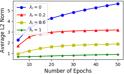
(a) Tweet

(b) BlogCatalog

(c) YouTube

Figure 1: Average $l_{2}$ Norm during SGD Optimization

SGD Optimization Results in Small Vector Norm: Figure 1 shows the average $l_{2}$ norm of the embedding vectors during the first 50 SGD epochs (with varying value of $\lambda_{r}$). As we can see, the average norm of embedding vectors increases consistently after each epoch, but the increase rate gets slower as time progresses. In practice, the SGD procedure is often stopped after $10\sim 50$ epochs (especially for large scale graphs with millions of vertices), and the relatively early stopping time would naturally result in small vector norm.

(a) Tweet

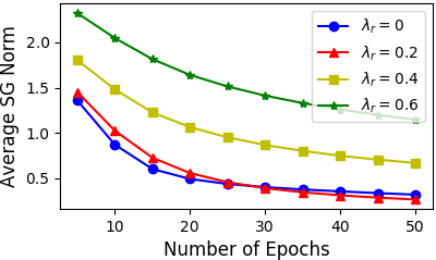
(b) BlogCatalog

(c) YouTube

Figure 2: Average Norm of Stochastic Gradients during SGD Optimization

The Vanishing Gradients: Figure 2 shows the average $l_{2}$ norm of the stochastic gradients $\partial L/\partial\mathbf{x}_{u}$ during the first 50 SGD epochs:

$$\frac{\partial L}{\partial\mathbf{x}_{u}}=-\sum_{v\in N_{+}(u)}\sigma(-\mathbf{x}_{u}^{T}\mathbf{x}_{v})\mathbf{x}_{v}+\sum_{v\in N_{-}(u)}\sigma(\mathbf{x}_{u}^{T}\mathbf{x}_{v})\mathbf{x}_{v}+2\lambda_{r}\mathbf{x}_{u}$$ (2)

From the figure, we can see that the stochastic gradients become smaller during the later stage of SGD, which is consistent with our earlier observation in Figure 1. This phenomenon can be intuitively explained as follows: after a few SGD epochs, most of the training data points have already been well fitted by the embedding vectors, which means that most of the coefficients $\sigma(\pm\mathbf{x}_{u}^{T}\mathbf{x}_{v})$ in Eqn (2) will be close to $0$ afterwards, and as a result the stochastic gradients will be small in the following epochs.

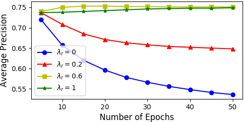
(a) Tweet (AP)

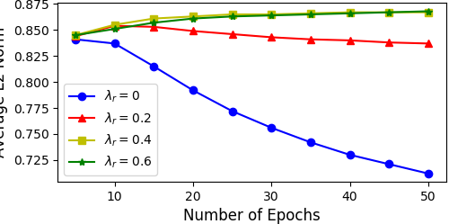
(b) BlogCatalog (AP)

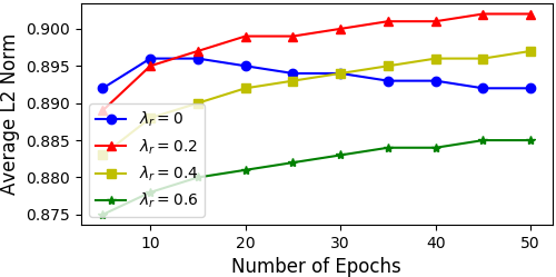
(c) YouTube (AP)

(d) BlogCatalog (F1)

Figure 3: Generalization Performance During SGD

Regularization and Early Stopping: Figure 3 shows the generalization performance of embedding vectors during the first 50 SGD epochs, in which we depicts the resulting average precision (AP) score for link prediction and F1 score for node label classification. As we can see, the generalization performance of embedding vectors starts to drop after $5\sim 20$ epochs when $\lambda_{r}$ is small, indicating that they are overfitting the training dataset afterwards. The generalization performance is worst near the end of SGD execution when $\lambda_{r}=0$, which coincides with the fact that embedding vectors in that case also have the largest norm among all settings. Thus, Figure 3 and Figure 1 collectively suggest that the generalization of linear graph embedding is determined by vector norm.

Impact of Embedding Dimension Choice: Figure 4 shows the generalization AP score on Tweet dataset with varying value of $\lambda_{r}$ and embedding dimension $D$. As we can see in Figure 4, without any norm regularization ($\lambda_{r}=0$), the embedding vectors will overfit the training dataset for any $D$ greater than $10$, which is consistent with our analysis in Claim 1. On the other hand, with larger $\lambda_{r}$, the impact of embedding dimension choice is significantly less noticeable, indicating that the primary factor for generalization is the vector norm in such scenarios.

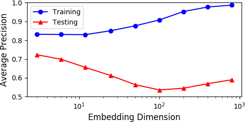
(a) $\lambda_{r}=0$

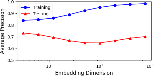
(b) $\lambda_{r}=0.2$

(c) $\lambda_{r}=0.6$

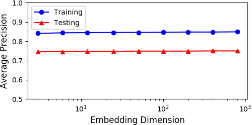
(d) $\lambda_{r}=1$

Figure 4: Impact of Embedding Dimension

4 Demonstrating the Importance of Norm Regularization via Hinge-Loss Linear Graph Embedding

In this section, we present the experimental results for a non-standard linear graph embedding formulation, which optimizes the following objective:

$$L= \lambda_{+1}\sum_{(u,v)\in E_{+}}h(\mathbf{x}_{u}^{T}\mathbf{x}_{v})+\lambda_{-1}\sum_{(u,v)\in E_{-}}h(-\mathbf{x}_{u}^{T}\mathbf{x}_{v})+\frac{\lambda_{r}}{2}\sum_{v\in V}||\mathbf{x}_{v}||_{2}^{2}$$ (3)

By replacing logistic loss with hinge-loss, it is now possible to apply the dual coordinate descent (DCD) method (Hsieh et al., 2008) for optimization, which circumvents the issue of vanishing gradients in SGD, allowing us to directly observe the impact of norm regularization. More specifically, consider all terms in Eqn (3) that are relevant to a particular vertex $u$:

$$L(u)=\sum\limits_{(\mathbf{x}_{i},y_{i})\in D}\frac{\lambda_{y_{i}}}{\lambda_{r}}\max(1-y_{i}\mathbf{x}_{u}^{T}\mathbf{x}_{i},0)+\frac{1}{2}\mathopen{\|}\mathbf{x}_{u}\mathclose{\|}^{2}.$$ (4)

in which we defined $D=\{(\mathbf{x}_{v},+1):v\in N_{+}(u)\}\cup\{(\mathbf{x}_{k},-1):k\in N_{-}(u)\}$. Since Eqn (4) takes the same form as a soft-margin linear SVM objective, with $\mathbf{x}_{u}$ being the linear coefficients and $(\mathbf{x}_{i},y_{i})$ being training data, it allows us to use any SVM solver to optimize Eqn (4), and then apply it asynchronously on the graph vertices to update their embeddings. The pseudo-code for the optimization procedure using DCD can be found in the appendix.

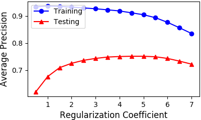
(a) Tweet

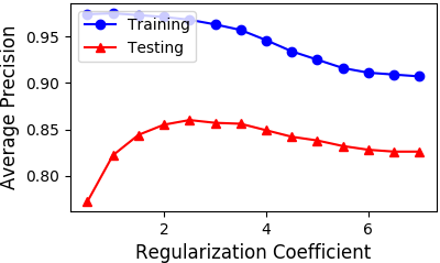
(b) BlogCatalog

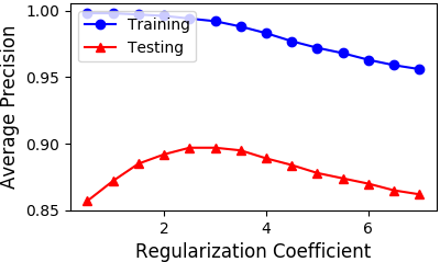
(c) YouTube

Figure 5: Generalization Average Precision with Varying $\lambda_{r}$ ($D=100$)

Impact of Regularization Coefficient: Figure 5 shows the generalization performance of embedding vectors obtained from DCD procedure ($\sim 20$ epochs). As we can see, the quality of embeddings vectors is very bad when $\lambda_{r}\approx 0$, indicating that proper norm regularization is necessary for generalization. The value of $\lambda_{r}$ also affects the gap between training and testing performance, which is consistent with our analysis that $\lambda_{r}$ controls the model capacity of linear graph embedding.

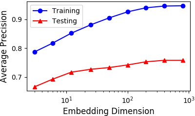
(a) Tweet

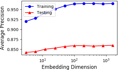
(b) BlogCatalog

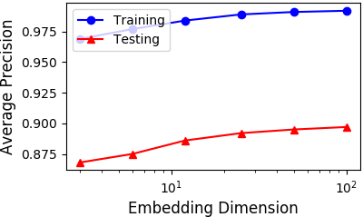
(c) YouTube

Figure 6: Generalization Average Precision with Varying $D$ ($\lambda_{r}=3$)

Impact of Embedding Dimension Choice: The choice of embedding dimension $D$ on the other hand is not very impactful as demonstrated in Figure 6: as long as $D$ is reasonably large ($\geq 30$), the exact choice has very little effect on the generalization performance. Even with extremely large embedding dimension setting $(D=1600)$. These results are consistent with our theory that the generalization of linear graph embedding is primarily determined by the norm constraints.

5 Discussion

So far, we have seen many pieces of evidence supporting our argument, suggesting that the generalization of embedding vectors in linear graph embedding is determined by the vector norm. Intuitively, it means that these embedding methods are trying to embed the vertices onto a small sphere centered around the origin point. The radius of the sphere controls the model capacity, and choosing proper embedding dimension allows us to control the trade-off between the expressive power of the model and the computation efficiency.

Note that the connection between norm regularization and generalization performance is actually very intuitive. To see this, let us consider the semantic meaning of embedding vectors: the probability of any particular edge $(u,v)$ being positive is equal to

$$\mathbf{Pr}(y=1|u,v)=\sigma(\mathbf{x}_{u}^{T}\mathbf{x}_{v})=\sigma(\frac{\mathbf{x}_{u}^{T}\mathbf{x}_{v}}{||\mathbf{x}_{u}||_{2}||\mathbf{x}_{v}||_{2}}||\mathbf{x}_{u}||_{2}||\mathbf{x}_{v}||_{2})$$

As we can see, this probability value is determined by three factors:

• $\mathbf{x}_{u}^{T}\mathbf{x}_{v}/(||\mathbf{x}_{u}||_{2}||\mathbf{x}_{v}||_{2})$, the cosine similarity between $\mathbf{x}_{u}$ and $\mathbf{x}_{v}$, evaluates the degree of agreement between the directions of $\mathbf{x}_{u}$ and $\mathbf{x}_{v}$.

• $||\mathbf{x}_{u}||_{2}$ and $||\mathbf{x}_{v}||_{2}$ on the other hand, reflects the degree of confidence we have regarding the embedding vectors of $u$ and $v$.

Therefore, by restricting the norm of embedding vectors, we are limiting the confidence level that we have regarding the embedding vectors, which is indeed intuitively helpful for preventing overfitting.

It is worth noting that our results in this paper do not invalidate the analysis of Levy & Goldberg (2014), but rather clarifies on some key points: as pointed out by Levy & Goldberg (2014), linear graph embedding methods are indeed approximating the factorization of PMI matrices. However, as we have seen in this paper, the embedding vectors are primarily constrained by their norm instead of embedding dimension, which implies that the resulting factorization is not really a standard low-rank one, but rather a low-norm factorization:

$$\mathbf{x}_{u}^{T}\mathbf{x}_{v}\approx\textit{PMI}(u,v)\quad\textit{s.t.}\quad\sum_{u}||\mathbf{x}_{u}||_{2}^{2}\leq C$$

The low-norm factorization represents an interesting alternative to the standard low-rank factorization, for which our current understanding of such factorization is still very limited. Given the empirical success of linear graph embedding methods, it would be really helpful if we can have a more in-depth analysis of such factorization, to deepen our understanding and potentially inspire new algorithms.

6 Conclusion

We have shown that the generalization of linear graph embedding methods are not determined by the dimensionality constraint but rather the norm of embedding vectors. We proved that limiting the norm of embedding vectors would lead to good generalization, and showed that the generalization of existing linear graph embedding methods is due to the early stopping of SGD and vanishing gradients. We experimentally investigated the impact embedding dimension choice, and demonstrated that such choice only matters when there is no norm regularization. In most cases, the best generalization performance is obtained by choosing the optimal value for the norm regularization coefficient, and in such case the impact of embedding dimension case is negligible. Our findings combined with the analysis of Levy & Goldberg (2014) suggest that linear graph embedding methods are probably computing a low-norm factorization of the PMI matrix, which is an interesting alternative to the standard low-rank factorization and calls for further study.

Appendix

Datasets and Experimental Protocols

We use the following three datasets in our experiments:

• Tweet is an undirected graph that encodes keyword co-occurrence relationships using Twitter data: we collected $\sim$1.1 million English tweets using Twitter’s Streaming API during 2014 August, and then extracted the most frequent 10,000 keywords as graph nodes and their co-occurrences as edges. All nodes with more than 2,000 neighbors are removed as stop words. There are 9,913 nodes and 681,188 edges in total.

• BlogCatalog (Zafarani & Liu, 2009) is an undirected graph that contains the social relationships between BlogCatalog users. It consists of 10,312 nodes and 333,983 undirected edges, and each node belongs to one of the 39 groups.

• YouTube (Mislove et al., 2007) is a social network among YouTube users. It includes 500,000 nodes and 3,319,221 undirected edges.

For each positive edge in training and testing datasets, we randomly sampled $4$ negative edges, which are used for learning the embedding vectors (in training dataset) and evaluating average precision (in testing dataset). In all experiments, $\lambda_{+}=1,\lambda_{-}=0.03$, which achieves the optimal generalization performance according to cross-validation. All initial coordinates of embedding vectors are uniformly sampled form $[-0.1,0.1]$.

Other Related Works

In the early days of graph embedding research, graphs are only used as the intermediate data model for visualization (Kruskal & Wish, 1978) or non-linear dimension reduction (Tenenbaum et al., 2000; Belkin & Niyogi, 2001). Typically, the first step is to construct an affinity graph from the features of the data points, and then the low-dimensional embedding of graph vertices are computed by finding the eigenvectors of the affinity matrix.

For more recent graph embedding techniques, apart from the linear graph embedding methods discussed in this paper, there are also methods (Wang et al., 2016; Kipf & Welling, 2016; Hamilton et al., 2017) that explore the option of using deep neural network structures to compute the embedding vectors. These methods typically try to learn a deep neural network model that takes the raw features of graph vertices to compute their low-dimensional embedding vectors: SDNE (Wang et al., 2016) uses the adjacency list of vertices as input to predict their Laplacian Eigenmaps; GCN (Kipf & Welling, 2016) aggregates the output of neighboring vertices in previous layer to serve as input to the current layer (hence the name “graph convolutional network”); GraphSage (Hamilton et al., 2017) extends GCN by allowing other forms of aggregator (i.e., in addition to the mean aggregator in GCN). Interestingly though, all these methods use only $2$ or $3$ neural network layers in their experiments, and there is also evidence suggesting that using higher number of layer would result in worse generalization performance (Kipf & Welling, 2016). Therefore, it still feels unclear to us whether the deep neural network structure is really helpful in the task of graph embedding.

Prior to our work, there are some existing research works suggesting that norm constrained graph embedding could generalize well. Srebro et al. (2005) studied the problem of computing norm constrained matrix factorization, and reported superior performance compared to the standard low-rank matrix factorization on several tasks. Given the connection between matrix factorization and linear graph embedding (Levy & Goldberg, 2014), the results in our paper is not really that surprising.

Proof of Theorem 1

Since $E_{\pm}$ consists of i.i.d. samples from $\mathcal{P}$, by the uniform convergence theorem (Bartlett & Mendelson, 2002; Shalev-Shwartz & Ben-David, 2014), with probability $1-\delta$:

$$\forall\mathbf{x},\quad\textit{s.t.}\quad\sum_{u\in U}\mathopen{\|}\mathbf{x}_{u}\mathclose{\|}^{2}\leq C_{U},\sum_{v\in V}\mathopen{\|}\mathbf{x}_{v}\mathclose{\|}^{2}\leq C_{V},$$

$$\mathbb{E}_{(a,b,y)\sim\mathcal{P}}l(y\mathbf{x}_{a}^{T}\mathbf{x}_{b})\leq\frac{1}{m+m^{\prime}}\sum_{i=1}^{m+m^{\prime}}l(y_{i}\mathbf{x}_{a_{i}}^{T}\mathbf{x}_{b_{i}})+2\mathcal{R}(\mathcal{H}_{C_{U},C_{V}})+4B\sqrt{\frac{2\ln(4/\delta)}{m+m^{\prime}}}$$

where $\mathcal{H}_{C_{U},C_{V}}=\{\mathbf{x}:\sum_{u\in U}\mathopen{\|}\mathbf{x}_{u}\mathclose{\|}^{2}\leq C_{U},\sum_{v\in V}\mathopen{\|}\mathbf{x}_{v}\mathclose{\|}^{2}\leq C_{V}\}$ is the hypothesis set, and $\mathcal{R}(\mathcal{H}_{C_{U},C_{V}})$ is the empirical Rademacher Complexity of $\mathcal{H}_{C_{U},C_{V}}$, which has the following explicit form:

$$\mathcal{R}(\mathcal{H}_{C_{U},C_{V}})=\frac{1}{m+m^{\prime}}\mathbb{E}_{\sigma_{a,b}\sim\{-1,1\}}\sup_{\mathbf{x}\in\mathcal{H}_{C_{U},C_{V}}}\sum_{i}\sigma_{a_{i},b_{i}}l(y_{i}\mathbf{x}_{a_{i}}^{T}\mathbf{x}_{b_{i}})$$

Here $\sigma_{a,b}$ are i.i.d. Rademacher random variables: $\mathbf{Pr}(\sigma_{a,b}=1)=\mathbf{Pr}(\sigma_{a,b}=-1)=0.5$. Since $l$ is $1$-Lipschitz, based on the Contraction Lemma (Shalev-Shwartz & Ben-David, 2014), we have:

$$\mathcal{R}(\mathcal{H}_{C_{U},C_{V}})\leq \frac{1}{m+m^{\prime}}\mathbb{E}_{\sigma_{a,b}\sim\{-1,1\}}\sup_{\mathbf{x}\in\mathcal{H}_{C_{U},C_{V}}}\sum_{i}\sigma_{a_{i},b_{i}}y_{i}\mathbf{x}_{a_{i}}^{T}\mathbf{x}_{b_{i}}$$

$$= \frac{1}{m+m^{\prime}}\mathbb{E}_{\sigma_{a,b}\sim\{-1,1\}}\sup_{\mathbf{x}\in\mathcal{H}_{C_{U},C_{V}}}\sum_{i}\sigma_{a_{i},b_{i}}\mathbf{x}_{a_{i}}^{T}\mathbf{x}_{b_{i}}$$

Let us denote $X_{U}$ as the $|U|d$ dimensional vector obtained by concatenating all vectors $\mathbf{x}_{u}$, and $X_{V}$ as the $|V|d$ dimensional vector obtained by concatenating all vectors $\mathbf{x}_{v}$:

$$X_{U}=(\mathbf{x}_{u_{1}},\mathbf{x}_{u_{2}},\ldots,\mathbf{x}_{u_{|U|}})\quad X_{V}=(\mathbf{x}_{v_{1}},\mathbf{x}_{v_{2}},\ldots,\mathbf{x}_{v_{|V|}})$$

Then we have:

$$||X_{U}||_{2}\leq\sqrt{C_{U}}\quad||X_{V}||_{2}\leq\sqrt{C_{V}}$$

The next step is to rewrite the term $\sum_{i}\sigma_{a_{i},b_{i}}\mathbf{x}_{a_{i}}^{T}\mathbf{x}_{b_{i}}$ in matrix form:

$$\sup_{\mathbf{x}\in\mathcal{H}_{C_{U},C_{V}}}\sum_{i}\sigma_{a_{i},b_{i}}\mathbf{x}_{a_{i}}^{T}\mathbf{x}_{b_{i}}$$

$$= \sup_{||X_{U}||_{2}\leq\sqrt{C_{U}},||X_{V}||_{2}\leq\sqrt{C_{V}}}X_{U}^{T}[A_{\sigma}\otimes I_{d}]X_{V}$$

$$= \sqrt{C_{U}}\mathopen{\|}A_{\sigma}\otimes I_{d}\mathclose{\|}_{2}\sqrt{C_{V}}$$

where $A\otimes B$ represents the Kronecker product of $A$ and $B$, and $||A||_{2}$ represents the spectral norm of $A$ (i.e., the largest singular value of $A$).

Finally, since $||A\otimes I||_{2}=||A||_{2}$, we get the desired result in Theorem 1.

Proof Sketch of Claim 1

We provide the sketch of a constructive proof here.

Firstly, we randomly initialize all embedding vectors. Then for each $v\in V$, consider all the relevant constraints to $\mathbf{x}_{v}$:

$$\mathbf{C}_{v}=\{(a,b,y)\in E:a=v\text{ or }b=v\}$$

Since $G$ is $d$-regular, $|\mathbf{C}_{v}|\leq d$. Therefore, there always exists vector $b\in\mathbb{R}^{d}$ satisfying the following $|C_{v}|$ constraints:

$$\forall(a,b,y)\in C_{v},y\mathbf{x}_{a}\mathbf{x}_{b}=1+\epsilon$$

as long as all the referenced embedding vectors are linearly independent.

Choose any vector $b^{\prime}$ in a small neighborhood of $b$ that is not the linear combination of any other $d-1$ embedding vectors (this is always possible since the viable set is a $d$-dimensional sphere minus a finite number of $d-1$ dimensional subspaces), and set $\mathbf{x}_{v}\leftarrow b^{\prime}$.

Once we have repeated the above procedure for every node in $V$, it is easy to see that all the constraints $y\mathbf{x}_{a}^{T}\mathbf{x}_{b}:(a,b,y)\in E$ are now satisfied.

Rough Estimation of $||A_{\sigma}||_{2}$ on Erdos–Renyi Graph

By the definition of spectral norm, $||A_{\sigma}||_{2}$ is equal to:

$$||A_{\sigma}||_{2}=\sup_{||\mathbf{x}||_{2}=||\mathbf{y}||_{2}=1,\mathbf{x},\mathbf{y}\in\mathbb{R}^{n}}\mathbf{y}^{T}A_{\sigma}\mathbf{x}$$

Note that,

$$\mathbf{y}^{T}A_{\sigma}\mathbf{x}=\sum_{(i,j)\in E}\sigma_{ij}y_{i}x_{j}$$

Now let us assume that the graph $G$ is generated from a Erdos-Renyi model (i.e., the probability of any pair $u,v$ being directed connected is independent), then we have:

$$\mathbf{y}^{T}A_{\sigma}\mathbf{x}=\sum_{i}\sum_{j}\sigma_{ij}e_{ij}y_{i}x_{j}$$

where $e_{ij}$ is the boolean random variable indicating whether $(i,j)\in E$.

By Central Limit Theorem,

$$\sum_{i}\sum_{j}\sigma_{ij}e_{ij}y_{i}x_{j}\sim\mathcal{N}(0,\frac{m}{n^{2}})$$

where $m$ is the expected number of edges, and $n$ is the total number of vertices. Then we have,

$$\mathbf{Pr}(\mathbf{y}^{T}A_{\sigma}\mathbf{x}\geq t)\approx O(e^{-\frac{t^{2}n^{2}}{2m}})$$

for all $||\mathbf{x}||_{2}=||\mathbf{y}||_{2}=1$.

Now let $S$ be an $\epsilon$-net of the unit sphere in $n$ dimensional Euclidean space, which has roughly $O(\epsilon^{-n})$ total number of points. Consider any unit vector $\mathbf{x},\mathbf{y}\in\mathbb{R}^{n}$, and let $\mathbf{x}_{S},\mathbf{y}_{S}$ be the closest point of $\mathbf{x},\mathbf{y}$ in $S$, then:

$$\mathbf{y}^{T}A_{\sigma}\mathbf{x}= (\mathbf{y}_{S}+\mathbf{y}-\mathbf{y}_{S})^{T}A_{\sigma}(\mathbf{x}_{S}+\mathbf{x}-\mathbf{x}_{S})$$

$$= \mathbf{y}_{S}^{T}A_{\sigma}\mathbf{x}_{S}+(\mathbf{y}-\mathbf{y}_{S})^{T}A_{\sigma}\mathbf{x}_{S}+\mathbf{y}_{S}^{T}A_{\sigma}(\mathbf{x}-\mathbf{x}_{S})+(\mathbf{y}-\mathbf{y}_{S})^{T}A_{\sigma}(\mathbf{x}-\mathbf{x}_{S})$$

$$\leq \mathbf{y}_{S}^{T}A_{\sigma}\mathbf{x}_{S}+2\epsilon n+\epsilon^{2}n$$

since $||A_{\sigma}||\leq n$ is always true.

By union bound, the probability that at least one pair of $\mathbf{x}_{S},\mathbf{y}_{S}\in S$ satisfying $\mathbf{y}_{S}^{T}A_{\sigma}\mathbf{x}_{S}\geq t$ is at most:

$$\mathbf{Pr}(\exists\mathbf{x}_{S},\mathbf{y}_{S}\in S:\mathbf{y}_{S}^{T}A_{\sigma}\mathbf{x}_{S}\geq t)\approx O(\epsilon^{-2n}e^{-\frac{t^{2}n^{2}}{2m}})$$

Let $\epsilon=1/n,t=\sqrt{8m\ln n/n}$, then the above inequality becomes:

$$\mathbf{Pr}(\exists\mathbf{x}_{S},\mathbf{y}_{S}\in S:\mathbf{y}_{S}^{T}A_{\sigma}\mathbf{x}_{S}\geq t)\approx O(e^{-n\ln n})$$

Since $\forall\mathbf{x}_{S},\mathbf{y}_{S}\in S,\mathbf{y}_{S}^{T}A_{\sigma}\mathbf{x}_{S}<t$ implies that

$$\sup_{||\mathbf{x}||_{2}=||\mathbf{y}||_{2}=1,\mathbf{x},\mathbf{y}\in\mathbb{R}^{n}}\mathbf{y}^{T}A_{\sigma}\mathbf{x}<t+2\epsilon n+\epsilon^{2}n$$

Therefore, we estimate $||A_{\sigma}||_{2}$ to be of order $O(\sqrt{m\ln n/n})$.

Pseudocode of Dual Coordinate Descent Algorithm

Algorithm 1 shows the full pseudo-code of the DCD method for optimizing the hinge-loss variant of linear graph embedding learning.

Algorithm 1 DCD Method for Hinge-Loss Linear Graph Embedding

function DcdUpdate($u,N_{+}(u),N_{-}(u)$)

     $D=\{(v,+1):v\in N_{+}(u)\}\cup\{(v,-1):v\in N_{-}(u)\}$

     $w\leftarrow\sum_{(v,s)\in D}\alpha_{uv}s\mathbf{x}_{v}$

     for $(v,s)\in D$ do

5:         $G\leftarrow sw^{T}\mathbf{x}_{v}-1$

         $U\leftarrow\lambda_{s}/\lambda_{r}$

         $PG\leftarrow\left\{\begin{array}[]{lr}\min(G,0)&\text{if }\alpha_{uv}=0\\ \max(G,0)&\text{if }\alpha_{uv}=U\\ G&\text{Otherwise}\end{array}\right.$

         if $PG\not=0$ then

              $Q=\mathbf{x}_{v}^{T}\mathbf{x}_{v}$

10:              $\bar{\alpha}_{uv}\leftarrow\alpha_{uv}$

              $\alpha_{uv}\leftarrow\min(\max(\alpha_{uv}-G/Q),0,U)$

              $w\leftarrow w+(\alpha_{uv}-\bar{\alpha}_{uv})sx_{v}$

         end if

     end for

15:     $\mathbf{x}_{u}\leftarrow w$

end function

function Main($V,E_{+},E_{-},\lambda_{+},\lambda_{-},\lambda_{r}$)

     Randomly initialize $\mathbf{x}_{v}$ for all $v\in V$

     Initialize $\alpha_{uv}\leftarrow 0$ for all $(u,v)\in E_{+}\cup E_{-}$

20:     for $t\in 1,\ldots,T$ do

         for $u\in V$ do

              $N_{+}(u)\leftarrow\{v\in V:(u,v)\in E_{+}\}$

              $N_{-}(u)\leftarrow\{v\in V:(u,v)\in E_{-}\}$

              DCDUpdate($u,N_{+}(u),N_{-}(u)$)

25:         end for

     end for

end function

References

- Bartlett & Mendelson (2002) Peter L Bartlett and Shahar Mendelson. Rademacher and gaussian complexities: Risk bounds and structural results. Journal of Machine Learning Research, 3(Nov):463–482, 2002.
- Belkin & Niyogi (2001) Mikhail Belkin and Partha Niyogi. Laplacian eigenmaps and spectral techniques for embedding and clustering. In NIPS, volume 14, pp. 585–591, 2001.
- Grover & Leskovec (2016) Aditya Grover and Jure Leskovec. node2vec: Scalable feature learning for networks. In KDD, pp. 855–864, 2016.
- Hamilton et al. (2017) Will Hamilton, Zhitao Ying, and Jure Leskovec. Inductive representation learning on large graphs. In Advances in Neural Information Processing Systems, pp. 1024–1034, 2017.
- Hsieh et al. (2008) Cho-Jui Hsieh, Kai-Wei Chang, Chih-Jen Lin, S. Sathiya Keerthi, and S. Sundararajan. A dual coordinate descent method for large-scale linear SVM. In ICML, pp. 408–415, 2008.
- Kipf & Welling (2016) Thomas N Kipf and Max Welling. Semi-supervised classification with graph convolutional networks. arXiv preprint arXiv:1609.02907, 2016.
- Kruskal & Wish (1978) Joseph B Kruskal and Myron Wish. Multidimensional scaling, volume 11. Sage, 1978.
- Levy & Goldberg (2014) Omer Levy and Yoav Goldberg. Neural word embedding as implicit matrix factorization. In Advances in neural information processing systems, pp. 2177–2185, 2014.
- Mikolov et al. (2013) Tomas Mikolov, Ilya Sutskever, Kai Chen, Gregory S. Corrado, and Jeffrey Dean. Distributed representations of words and phrases and their compositionality. In NIPS, pp. 3111–3119, 2013.
- Mislove et al. (2007) Alan Mislove, Massimiliano Marcon, Krishna P. Gummadi, Peter Druschel, and Bobby Bhattacharjee. Measurement and Analysis of Online Social Networks. In Proceedings of the 5th ACM/Usenix Internet Measurement Conference (IMC’07), San Diego, CA, October 2007.
- Perozzi et al. (2014) Bryan Perozzi, Rami Al-Rfou, and Steven Skiena. Deepwalk: Online learning of social representations. In KDD, pp. 701–710, 2014.
- Qiu et al. (2018) Jiezhong Qiu, Yuxiao Dong, Hao Ma, Jian Li, Kuansan Wang, and Jie Tang. Network embedding as matrix factorization: Unifying deepwalk, line, pte, and node2vec. In Proceedings of the Eleventh ACM International Conference on Web Search and Data Mining, pp. 459–467. ACM, 2018.
- Shalev-Shwartz & Ben-David (2014) Shai Shalev-Shwartz and Shai Ben-David. Understanding machine learning: From theory to algorithms. Cambridge university press, 2014.
- Srebro et al. (2005) Nathan Srebro, Jason Rennie, and Tommi S Jaakkola. Maximum-margin matrix factorization. In Advances in neural information processing systems, pp. 1329–1336, 2005.
- Tang et al. (2015a) Jian Tang, Meng Qu, and Qiaozhu Mei. Pte: Predictive text embedding through large-scale heterogeneous text networks. In KDD, pp. 1165–1174, 2015a.
- Tang et al. (2015b) Jian Tang, Meng Qu, Mingzhe Wang, Ming Zhang, Jun Yan, and Qiaozhu Mei. Line: Large-scale information network embedding. In WWW, pp. 1067–1077, 2015b.
- Tenenbaum et al. (2000) Joshua B Tenenbaum, Vin De Silva, and John C Langford. A global geometric framework for nonlinear dimensionality reduction. science, 290(5500):2319–2323, 2000.
- Wang et al. (2016) Daixin Wang, Peng Cui, and Wenwu Zhu. Structural deep network embedding. In KDD, pp. 1225–1234. ACM, 2016.
- Wang et al. (2015) Sheng Wang, Hyunghoon Cho, ChengXiang Zhai, Bonnie Berger, and Jian Peng. Exploiting ontology graph for predicting sparsely annotated gene function. Bioinformatics, 31(12):i357–i364, 2015.
- Zafarani & Liu (2009) R. Zafarani and H. Liu. Social computing data repository at ASU, 2009. URL http://socialcomputing.asu.edu.