A generalized matrix Krylov subspace method for TV regularization

Abstract

This paper presents an efficient algorithm to solve total variation (TV) regularizations of images contaminated by a both blur and noise. The unconstrained structure of the problem suggests that one can solve a constrained optimization problem by transforming the original unconstrained minimization problem to an equivalent constrained minimization one. An augmented Lagrangian method is developed to handle the constraints when the model is given with matrix variables, and an alternating direction method (ADM) is used to iteratively find solutions. The solutions of some sub-problems are belonging to subspaces generated by application of successive orthogonal projections onto a class of generalized matrix Krylov subspaces of increasing dimension.

1 Introduction

In this paper we consider the solution of the following matrix equation

$$B=H_{2}XH_{1}^{T},$$ (1)

where $B$ is generally contaminated by noise. $H_{1}$ and $H_{2}$ are matrices of ill-determined rank, which makes the solution $X$ very sensitive to perturbations in $B$. Discrete ill-posed problems of the form (1) arise, for instance, from the discretization of Fredholm integral equations of the first kind in two space-dimensions,

$$\int\int_{\Omega}K(x,y,s,t)f(s,t)dsdt=g(x,y),\qquad(x,y)\in\Omega^{\prime},$$ (2)

where $\Omega$ and $\Omega^{\prime}$ are rectangles in $\mathbb{R}^{2}$ and the kernel is separable

$$K(x,y,s,t)=k_{1}(x,s)k_{2}(y,t),\quad(x,y)\in\Omega^{\prime},\quad(s,t)\in\Omega,$$

The aim of this work is to solve this problem with application to one single channel and multichannel images.

1.1 Single channel images

For single channel images we seek to recover an unknown vector from limited information. This problem is mathematically formulated as the following model

$$b=Hx,$$ (3)

where $x\in\mathbb{R}^{mn}$ is a vector denoting the unknown solution, $b\in\mathbb{R}^{mn}$ is a vector denoting the observed data contaminated by noise and $H\in\mathbb{R}^{mn\times mn}$ is a linear map. The problem arises, for instance in image restoration [1, 2, 6, 15, 16]. In this paper we focus on the application to image restoration in which $x$ represents the unknown sharp image that is to be estimated from its blurry and noisy observation $b$. The matrix $H$ is the blurring operator characterized by a PSF describing this blur. Due to the ill-conditioning of the matrix $H$ and the presence of the noise, the problem (3) cannot be easily solved which means that the minimization of only the fidelity term typically yields a meaningless computed solution. Therefore, to stabilise the recovered image, regularization is needed. There are several techniques to regularize the linear inverse problem given by equation (3) ; see for example, [9, 27, 23, 26]. All of these techniques stabilize the restoration process by adding a regularization term, depending on some a priori knowledge of the unknown image, resulting in the model

$$\underset{x}{\text{min}}\{\|Hx-b\|^{p}_{p}+\mu\|\Phi(x)\|^{q}_{q}\},$$ (4)

where $\Phi(x)$ is the regularizer that enforces the a priori knowledge and the parameter $\mu$ is used to balance the two terms. This problem is referred to as $\ell_{p}-\ell_{q}$ minimization problem. Different choices of $\Phi(x)$, $p$ and $q$ lead to a wide variety of regularizers. Among them we find the well known Tikhonov regularization, where $\Phi$ is the identity matrix, $p=2$ and $q=2$, see for example [27]. If the goal is to enforce sparsity on the solution, one can also consider $\Phi=I$, $p=2$ and $q=1$. Another well-known class of regularizers are based on total variation (TV), which is a better choice if the goal is to preserve sharp edges. In this case one let $\Phi$ to be the discrete gradient operator, see [23]. The problem (4) has been studied in many papers to propose nonlinear optimization algorithms that can deal with the nonlinear properties of this problem; see for example [25, 28]. These techniques are computationally demanding if the main cost of computation is the matrix-vector multiplication (MVM). It is our main goal to recover a good approximation of the unknown sharp image at low computational cost. Because of some unique features in images, we seek an image restoration algorithm that utilizes blur information, exploits the spatially invariant properties. For this reason we suppose that the PSF is identical in all parts of the image and separates into horizontal and vertical components. Then the matrix $H$ is the Kronecker product of two matrices $H_{1}$ and $H_{2}$,

$$H=H_{1}\otimes H_{2}=\begin{bmatrix}h_{1,1}^{(1)}H_{2}&h_{1,2}^{(1)}H_{2}&\cdots&h_{1,n}^{(1)}H_{2}\\ h_{2,1}^{(1)}H_{2}&h_{2,2}^{(1)}H_{2}&\cdots&h_{2,n}^{(1)}H_{2}\\ \vdots&\vdots&&\vdots\\ h_{n,1}^{(1)}H_{2}&h_{n,2}^{(1)}H_{2}&\cdots&h_{n,n}^{(1)}H_{2}\end{bmatrix}.$$ (5)

In what follows we will need the vec and mat notations, which are a useful tools in transforming the expression of matrix-vector product into a matrix-matrix product. Let the operator vec transform a matrix $A=[a_{i,j}]\in\mathbb{R}^{m\times n}$ to a vector $a\in\mathbb{R}^{mn}$ by stacking the columns of $A$ from left to right, i.e,

$$a=[a_{1,1},a_{2,1},\ldots,a_{m,1},a_{1,2},a_{2,2},\ldots,a_{m,2},\ldots,a_{m,n}]^{T},$$ (6)

and let mat be the inverse operator, which transforms a vector (6) to an associated matrix $A=[a_{i,j}]\in\mathbb{R}^{m\times n}$. Thus,

$$\textsf{vec}(A)=a,\qquad\textsf{mat}(a)=A.$$

The Kronecker product satisfies the following relations for matrices $A,B,C,D,X$ of suitable sizes:

$$\left.\begin{array}[]{rcl}(A\otimes B)\textsf{vec}(X)&=&\textsf{vec}(BXA^{T}),\\ (A\otimes B)^{T}&=&A^{T}\otimes B^{T},\\ (AB)\otimes(CD)&=&(A\otimes C)(B\otimes D).\end{array}\right\}$$ (7)

For $A,B\in\mathbb{R}^{m\times n}$, we define the inner product

$$\langle A,B\rangle_{F}:=\textsf{tr}(A^{T}B),$$ (8)

where $\textsf{tr}(\cdot)$ denotes the trace. Notice that

$$\langle A,B\rangle_{F}=(\textsf{vec}(A))^{T}\textsf{vec}(B).$$ (9)

The Frobenius norm is associated with this inner product,

$$\|A\|_{F}:=\langle A,A\rangle_{F}^{1/2},$$

and it satisfies

$$\|A\|_{F}=\|\textsf{vec}(A)\|_{2}.$$ (10)

By using the properties (7), the equation (3) can be rewritten as

$$B=H_{2}XH_{1}^{T},$$ (11)

where $X=\textsf{mat}(x)$ and $B=\textsf{mat}(b)$, which yields the model (1).

1.2 Multichannel Images

Recovering multichannel images from their blurry and noisy observations can be seen as a linear system of equations with multiple right-hand sides. The most commonly multichannel images is the RGB representation, which uses three channels; see [11, 15]. It should be pointed out that the algorithms proposed in this paper can be applied to the solution of Fredholm integral equations of the first kind in two or more space dimensions and to the restoration of hyper-spectral images. The latter kind of images generalize color images in that they allow more than three “colors”; see, e.g., [20]. If the channels are represented by $m\times n$ pixels, the full blurring model is described by the following form

$$b=Hx,$$ (12)

where $b$ and $x$ in $\mathbb{R}^{kmn}$, represent the blurred and noisy multichannel image and the original image respectively. For an image with $k$ channels, they are given by

$$b=[b^{(1)};b^{(2)};...;b^{(k)}],\quad x=[x^{(1)};x^{(2)};...;x^{(k)}],$$

where $b^{(i)}$ and $x^{(i)}$ in $\mathbb{R}^{mn}$ are obtained by stacking the columns of each channel on top of each other. The $kmn\times kmn$ multichannel blurring matrix $H$ is given by

$$H=H_{1}\otimes H_{2},$$ (13)

The matrix $H_{2}\in\mathbb{R}^{mn\times mn}$ represents the same within-channel blurring in all the $k$ channels. The matrix $H_{1}$ of dimension $k\times k$ models the cross-channel blurring, which is the same for all pixels in the case of a spatially invariant blur. If $H_{1}=I$, the blurring is said to be within-channel. If no colour blurring arises (i.e., $H_{1}=I$), then $k$ independent deblurring problems are solved; hence the spatially invariant blurring model is given by

$$b_{i}=H_{2}x_{i},\quad i=1,...,k.$$ (14)

In this case, the goal is to model the blurring of $k$ channels image as a linear system of equations with $k$ right-hand sides. For this reason we let $B$ and $X$ in $\mathbb{R}^{mn\times k}$ to be denoted by $\left[b^{(1)},b^{(2)},...,b^{(k)}\right]$ and $\left[x^{(1)},x^{(2)},...,x^{(k)}\right]$, respectively. The optical blurring is then modeled by

$$B=H_{2}X,$$ (15)

which yields the model (1) with $H_{1}=I$. When the spatially invariant cross-channel is present (i.e., $H_{1}\neq I$) and by using the Kronecker product properties, the following blurring model is to be solved

$$B=H_{2}XH_{1}^{T},$$ (16)

which also yields the model (1). Introduce the linear operator

$$\mathcal{H}:\mathbb{R}^{p\times q} \rightarrow \mathbb{R}^{p\times q}$$

$$\mathcal{H}(X) = H_{2}XH_{1}^{T}.$$

Its transpose is given by $\mathcal{H}^{T}(X)=H_{2}^{T}XH_{1}$. The problem (1) can be then expressed as

$$B=\mathcal{H}(X).$$

The total variation regularization is known to be the most popular and effective techniques for the images restoration. Given an image defined as a function $u:\Omega\longrightarrow\mathbb{R}$, where $\Omega$ is a bounded open subset of $\mathbb{R}^{2}$, the total variation (TV) of $u$ can be defined as

$$\text{TV}_{k}(u)=\int_{\Omega}\|\nabla u(x)\|_{k}dx,$$ (17)

where $\nabla$ denotes the gradient of $u$ and $\|.\|_{k}$ is a norm in $\mathbb{R}^{2}$. When $u$ is represented by $m\times n$ image $X$, a discrete form of (17) is always used, given by

$$\text{TV}_{1}(X)=\sum_{i=1}^{m}\sum_{j=1}^{n}\left(|\left(D_{1,n}X\right)_{ij}|+|\left(D_{1,m}X\right)_{ij}|\right)$$ (18)

in the anisotropic total variation case, or

$$\text{TV}_{2}(X)=\sum_{i=1}^{m}\sum_{j=1}^{n}\sqrt{\left(\left(D_{1,n}X\right)^{2}_{ij}+\left(D_{1,m}X\right)^{2}_{ij}\right)}$$ (19)

in the isotropic total variation case. $D_{1,m}$ and $D_{1,n}$ denote the finite difference approximations of the horizontal and vertical first derivative operators, respectively, and they are defined as follows

$$\begin{pmatrix}D_{1,n}\\ D_{1,m}\end{pmatrix}X=\begin{pmatrix}CX\\ XC^{T}\end{pmatrix},$$ (20)

where

$$C:=\begin{bmatrix}-1&1&&\\ &\ddots&\ddots&\\ &&-1&1\end{bmatrix}\in\mathbb{R}^{d-1\times d},$$

where $d$ is the number of pixels in each row and column of the image considered. For the ill-posed image restoration problem (1), the resulting matrices $H_{1}$ and $H_{2}$ are ill-conditioned. By regularization of the problem (1), we solve as a special case one of the following matrix problems:

$$\underset{X}{\text{min}}\left(\|\mathcal{H}(X)-B\|_{F}^{2}+\mu\text{TV}_{k}(X)\right),\quad k=1,2$$ (21)

or

$$\underset{X}{\text{min}}\left(\|\mathcal{H}(X)-B\|_{1,1}+\mu\text{TV}_{k}(X)\right)\quad k=1,2.$$ (22)

where $\|.\|_{1,1}$ is the $\ell_{1}$ norm and $\mu$ is a regularization parameter. Problems (21) and (22) are refereed to as TV/L2 and TV/L1 minimization, respectively.

2 TV/L2 minimization problem

In this section we consider the solution of the following TV/L2 minimization problem

$$\underset{X}{\text{min}}\left(\|\mathcal{H}(X)-B\|_{F}^{2}+\mu\text{TV}_{2}(X)\right).$$ (23)

The model (23) is very difficult to solve directly due to the non-differentiability and non-linearity of the TV term. It is our goal to develop an efficient TV minimization scheme to handle this problem. The core idea is based on augmented Lagrangian method (ALM) [13, 22] and alternating direction method (ADM) [8]. The idea of ALM is to transform the unconstrained minimization task (23) into an equivalent constrained optimization problem, and then add a quadratic penalty term instead of the constraint violation with the multipliers. The idea of ADM is to decompose the transformed minimization problem into three easier and smaller sub-problems such that some involved variables can be minimized separately and alternatively. Let us begin by considering the equivalent equality-constrained problem of (23). We first notice that the minimization problem (23) can be rewritten as

$$\underset{X,M^{(n)},M^{(m)}}{\text{min}}\left(\|\mathcal{H}(X)-B\|_{F}^{2}+\mu\sum_{i=1}^{m}\sum_{j=1}^{n}\|M_{i,j}\|_{2}\right),$$ (24)

$$\text{subject to}\quad D_{1,n}X=M^{(n)},\quad D_{1,m}X=M^{(m)}.$$

where $M_{i,j}=\left[\left(D_{1,n}X\right)_{ij},\left(D_{1,m}X\right)_{ij}\right]$. If we set $M_{i,j}^{(n)}=\left(D_{1,n}X\right)_{ij}$ and $M_{i,j}^{(m)}=\left(D_{1,m}X\right)_{ij}$ This constrained problem can be also formulated as

$$\underset{}{\text{min}}\quad F(X)+G(Y),$$ (25)

$$\text{subject to}\quad DX=Y,$$

where,

$$F(X)=\|\mathcal{H}(X)-B\|_{F}^{2},\quad G(Y)=\mu\sum_{i=1}^{m}\sum_{j=1}^{n}\|M_{i,j}\|_{2},\quad D=\begin{pmatrix}D_{1,n}\\ D_{1,m}\end{pmatrix},\quad Y=\begin{pmatrix}M^{(n)}\\ M^{(m)}\end{pmatrix}$$

The augmented Lagrangian function of (25) is defined as

$$\mathcal{L}_{\beta}\left(X,Y,Z\right)=F(X)+G(Y)+\left<DX-Y,Z\right>+\frac{\beta}{2}\|DX-Y\|_{F}^{2},$$ (26)

where $Z\in\mathbb{R}^{2m\times n}$ is the Lagrange multiplier of the linear constraint and $\beta>0$ is the penalty parameter for the violation of this linear constraint.
To solve the nonlinear problem (23), we find the saddle point of the Lagrangian (26) by using the ADM method. The idea of this method is to apply an alternating minimization iterative procedure, namely, for $k=0,1,...,$ we solve

$$(X_{k+1},Y_{k+1})=\underset{X}{\text{arg min }}\mathcal{L}_{\beta}(X,Y,Z_{k}).$$ (27)

The Lagrange multiplier is updated by

$$Z_{k+1} = Z_{k}+\beta\left(DX_{k+1}-Y_{k+1}\right).$$ (28)

2.1 Solving the Y-problem

Given $X$, $Y_{k+1}$ can be obtained by solving

$$\underset{Y}{\text{ min }}\mu\sum_{i=1}^{m}\sum_{j=1}^{n}\|M_{i,j}\|_{2}+\frac{\beta}{2}\|DX-Y\|_{F}^{2}+\left<DX-Y,Z_{k}\right>_{F}$$ (29)

which is equivalent to solve

$$\underset{Y}{\text{ min }}\mu\sum_{i=1}^{m}\sum_{j=1}^{n}\|M_{i,j}\|_{2}+\frac{\beta}{2}\left\|\begin{pmatrix}M^{(n)}\\ M^{(m)}\end{pmatrix}-\begin{pmatrix}D_{1,n}X\\ D_{1,m}X\end{pmatrix}-\frac{1}{\beta}\begin{pmatrix}Z^{(1)}_{k}\\ Z^{(2)}_{k}\end{pmatrix}\right\|_{F}^{2}$$ (30)

which is also equivalent to solve the so-called M-subproblem

$$\underset{M_{i,j}}{\text{ min }}\sum_{i=1}^{m}\sum_{j=1}^{n}\mu\|M_{i,j}\|_{2}+\frac{\beta}{2}\left|M^{(n)}_{ij}-K_{ij}\right|_{F}^{2}+\frac{\beta}{2}\left|M^{(m)}_{ij}-L_{ij}\right|_{F}^{2}$$ (31)

where $K_{ij}=\left(D_{1,n}X\right)_{ij}+\frac{1}{\beta}\left(Z^{(1)}_{k}\right)_{ij}$ and $L_{ij}=\left(D_{1,m}X\right)_{ij}+\frac{1}{\beta}\left(Z^{(2)}_{k}\right)_{ij}$. To solve (31) we use following well-known two dimensional shrinkage formula [18]

$$\textbf{Shrink}(y,\gamma,\delta)=\text{max}\left\{\left\|y+\frac{\gamma}{\delta}\right\|_{2}-\frac{1}{\delta},0\right\}\frac{y+\gamma/\delta}{\|y+\gamma/\delta\|_{2}},$$ (32)

where the convention 0·(0/0) = 0 is followed. The solution of (31) is then given by

$$M_{i,j}=\text{max}\left\{\|T_{i,j}\|_{2}-\frac{\mu}{\beta},0\right\}\frac{T_{i,j}}{\|T_{i,j}\|_{2}},$$ (33)

where $T_{i,j}=\left[\left(D_{1,n}X_{k}\right)_{i,j}+\frac{1}{\beta}\left(Z^{(1)}_{k}\right)_{i,j},\left(D_{1,m}X_{k}\right)_{i,j}+\frac{1}{\beta}\left(Z^{(2)}_{k}\right)_{i,j}\right].$
For the anisotropic case we solve the following problem

$$\underset{M_{i,j}}{\text{ min }}\sum_{i=1}^{m}\sum_{j=1}^{n}\mu\|M_{i,j}\|_{1}+\frac{\beta}{2}\left|M^{(n)}_{ij}-K_{ij}\right|_{F}^{2}+\frac{\beta}{2}\left|M^{(m)}_{ij}-L_{ij}\right|_{F}^{2}$$ (34)

which can be also solved by the one dimensional shrinkage formula. This gives

$$M^{(n)}_{ij} = \text{max}\left\{K_{ij}-\frac{\mu}{\beta},0\right\}.\text{sign}\left(K_{ij}\right),$$ (35)

$$M^{(m)}_{ij} = \text{max}\left\{L_{ij}-\frac{\mu}{\beta},0\right\}.\text{sign}\left(L_{ij}\right),$$ (36)

2.2 Solving the X-problem

Given $Y$, $X_{k+1}$ can be obtained by solving

$$\underset{X}{\text{min }}\frac{\beta}{2}\|DX-Y\|_{F}^{2}+\left<DX-Y,Z_{k}\right>_{F}+\|\mathcal{H}(X)-B\|_{F}^{2}.$$ (37)

This problem can be also solved by considering the following normal equation

$$H_{1}^{T}H_{1}XH_{2}^{T}H_{2}+\beta D^{T}DX=H_{1}^{T}BH_{2}+D^{T}\left(\beta Y-Z_{k}\right).$$ (38)

The linear matrix equation can be rewritten in the following form

$$A_{1}XA_{2}+A_{3}XA_{4}=E_{k},\quad k=1,...,$$ (39)

where $A_{1}=H_{1}^{T}H_{1}$, $A_{2}=H_{2}^{T}H_{2}$, $A_{3}=\beta D^{T}D$, $A_{4}=I$ and $E_{k}=H_{1}^{T}BH_{2}+D^{T}\left(\beta Y-Z_{k}\right)$. The equation (39) is refereed to as the generalized Sylvester matrix equation. We will see in section 4 how to compute approximate solutions to those matrix equations

2.3 Convergence analysis of TV/L2 problem

For the vector case, many convergence results have been proposed in the literature ; see for instance [10, 14]. For completeness, we give a proof here for the matrix case. A function $\Psi$ is said to be proper if the domain of $\Psi$ denoted by $\textbf{dom}\Psi:=\left\{U\in\mathbb{R}^{p\times q},\Psi(U)<\infty\right\}$ is not empty. For the problem (25), $F$ and $G$ are closed proper convex functions. According to [7, 24], the problem (25) is solvable, i.e., there exist $X_{*}$ and $Y_{*}$, not necessarily unique that minimize (25). Let $\mathcal{W}=\Omega\times\mathcal{Y}\times\mathbb{R}^{p\times q}$, where $\Omega$ and $\mathcal{Y}$ are given closed and convex nonempty sets. The saddle-point problem is equivalent to finding $(X_{*},Y_{*},Z_{*})\in\mathcal{W}$ such that

$$\mathcal{L}_{\beta}(X_{*},Y_{*},Z)\leq\mathcal{L}_{\beta}(X_{*},Y_{*},Z_{*})\leq\mathcal{L}_{\beta}(X,Y,Z_{*}),\qquad\forall\left(X,Y,Z\right)\in\mathcal{W}.$$ (40)

The properties of the relation between the saddle-points of $\mathcal{L}_{\beta}$ and $\mathcal{L}_{0}$ and the solution of (25) are stated by the following theorem from [10]

Theorem 1.

$(X_{*},Y_{*},Z_{*})$ is a saddle-point of $\mathcal{L}_{0}$ if and only if $(X_{*},Y_{*},Z_{*})$ is a saddle-point of $\mathcal{L}_{\beta}$ $\forall\beta>0$. Moreover $(X_{*},Y_{*})$ is a solution of (25).

We will see in what follows how this theorem can be used to give the convergence of $\left(X_{k+1},Y_{k+1}\right)$. It should be pointed out that the idea of our proof follows the convergence results in [5].

Theorem 2.

Assume that $(X_{*},Y_{*},Z_{*})$ is a saddle-point of $\mathcal{L}_{\beta}$ $\forall\beta>0$. The sequence $(X_{k+1},Y_{k+1},Z_{k+1})$ generated by Algorithm 1 satisfies

1. $\lim\limits_{k\rightarrow+\infty}F(X_{k+1})+G(Y_{k+1})=F(X_{*})+G(Y_{*})$,

2. $\lim\limits_{k\rightarrow+\infty}\|DX_{k+1}-Y_{k+1}\|_{F}=0,$

Proof  In order to show the convergence of this theorem, it suffice to show that the non-negative function

$$F^{k}=\frac{1}{\beta}\|Z_{k}-Z_{*}\|_{F}^{2}+\beta\|X_{k}-X_{*}\|_{F}^{2}$$ (41)

decreases at each iteration. Let us define $S_{k}$, $M_{k}$ and $M_{*}$ as

$$S_{k}=DX_{k}-Y_{k},\quad M_{k}=F(X_{k})+G(Y_{k}),\quad M_{*}=F(X_{*})+G(Y_{*}).$$

In the following we show

$$F^{k+1}\leq F^{k}-\beta\|S_{k+1}\|_{F}^{2}-\beta\|Y_{k+1}-Y_{k}\|_{F}^{2}.$$ (42)

Since $(X_{*},Y_{*},Z_{*})$ is a saddle-point of $\mathcal{L}_{\beta}$ $\forall\beta>0$, it follows from Theorem 1 that $(X_{*},Y_{*},Z_{*})$ is also a saddle-point of $\mathcal{L}_{0}$. This is characterized by

$$\mathcal{L}_{0}(X_{*},Y_{*},Z)\leq\mathcal{L}_{0}(X_{*},Y_{*},Z_{*})\leq\mathcal{L}_{0}(X,Y,Z_{*}),\qquad\forall\left(X,Y,Z\right)\in\mathcal{W}.$$ (43)

From the second inequality of (43), we have

$$M_{*}-M_{k+1}\leq\left<S_{k+1},Z_{*}\right>_{F}.$$ (44)

In the oder hand, $X_{k+1}$ is a minimizer of $\mathcal{L}_{\beta}$ $\forall\beta>0$, this implies that the optimality conditions reads

$$2\mathcal{H}^{T}\left(\mathcal{H}(X_{k+1})-B\right)+D^{T}(Z_{k}+\beta(DX_{k+1}-Y_{k}))=0.$$ (45)

By plugging $Z_{k}=Z_{k+1}-\beta(DX_{k+1}-Y_{k+1})$ and rearranging we obtain

$$2\mathcal{H}^{T}\left(\mathcal{H}(X_{k+1})-B\right)+D^{T}(Z_{k+1}-\beta(Y_{k+1}-Y_{k}))=0,$$ (46)

which means that $X_{k+1}$ minimizes

$$F(X)+\left<Z_{k+1}+\beta(Y_{k+1}-Y_{k}),DX\right>_{F}.$$ (47)

It follows that

$$F(X_{k+1})-F(X_{*})\leq\left<Z_{k+1}+\beta(Y_{k+1}-Y_{k}),DX_{*}\right>_{F}-\left<Z_{k+1}+\beta(Y_{k+1}-Y_{k}),DX_{k+1}\right>_{F}.$$ (48)

A similar argument shows that

$$G(Y_{k+1})-G(Y_{*})\leq\left<Z_{k+1},Y_{k+1}\right>-\left<Z_{k+1},Y_{*}\right>_{F}.$$ (49)

Adding (48) and (49) and using $DX_{*}=Y_{*}$ implies

$$M_{k+1}-M_{*}\leq-\left<S_{k+1},Y_{k+1}\right>_{F}-\left<\beta(Y_{k+1}-Y_{k}),S_{k+1}+(Y_{k+1}-Y_{*})\right>_{F}.$$ (50)

Adding (44) and (50) and multiplying through by 2 gives

$$2\left<S_{k+1},Z_{k+1}-Z_{*}\right>_{F}+2\left<\beta(Y_{k+1}-Y_{k}),S_{k+1}\right>_{F}+2\left<\beta(Y_{k+1}-Y_{k}),(Y_{k+1}-Y_{*})\right>_{F}\leq 0$$ (51)

The inequality (42) will hold by rewriting each term of the inequality (51). Let us begin with its first term. Substituting $Z_{k+1}=Z_{k}+\beta S_{k+1}$ gives

$$2\left<S_{k+1},Z_{k+1}-Z_{k}\right>_{F}=2\left<S_{k+1},Z_{k}-Z_{*}\right>_{F}+\beta\|S_{k+1}\|_{F}^{2}+\beta\|S_{k+1}\|_{F}^{2}.$$ (52)

Since $S_{k+1}=\frac{1}{\beta}\left(Z_{k+1}-Z_{k}\right)$, it follows that the first two terms of the right hand side of (52) can be written as

$$\frac{2}{\beta}\left<Z_{k+1}-Z_{k},Z_{k}-Z_{*}\right>_{F}+\frac{1}{\beta}\|Z_{k+1}-Z_{k}\|_{F}^{2}.$$ (53)

Substituting $Z_{k+1}-Z_{k}=(Z_{k+1}-Z_{*})-(Z_{k}-Z_{*})$, shows that (53) can be written as

$$\frac{1}{\beta}\left(\|Z_{k+1}-Z_{*}\|_{F}^{2}-\|Z_{k}-Z_{*}\|_{F}^{2}\right).$$ (54)

We turn now to the remaining terms, i.e.,

$$\beta\|S_{k+1}\|_{F}^{2}+2\left<\beta(Y_{k+1}-Y_{k}),S_{k+1}\right>_{F}+2\left<\beta(Y_{k+1}-Y_{k}),(Y_{k+1}-Y_{*})\right>_{F}$$ (55)

Substituting $Y_{k+1}-Y_{*}=(Y_{k+1}-Y_{k})+(Y_{k+1}-Y_{*})$ shows that (55) can be expressed as

$$\beta\|S_{k+1}+(Y_{k+1}-Y_{k})\|_{F}^{2}+\beta\|Y_{k+1}-Y_{k}\|_{F}^{2}+2\beta\left<Y_{k+1}-Y_{k},Y_{k}-Y_{*}\right>_{F}.$$ (56)

Substituting $Y_{k+1}-Y_{k}=(Y_{k+1}-Y_{*})-(Y_{k}-Y_{*})$ in the last two terms shows that (56) can be expressed as

$$\beta\|S_{k+1}+(Y_{k+1}-Y_{k})\|_{F}^{2}+\beta\left(\|Y_{k+1}-Y_{*}\|_{F}^{2}-\|Y_{k}-Y_{*}\|_{F}^{2}\right)$$ (57)

Using (54) and (57) shows that (51) can be expressed as

$$F^{k}-F^{k+1}\geq\beta\|S_{k+1}+(Y_{k+1}-Y_{k})\|_{F}^{2}.$$ (58)

To show (42), it is now suffice to show that $2\beta\left<S_{k+1},Y_{k+1}-Y_{k}\right>_{F}\geq 0$. Since $(X_{k},Y_{k},Z_{k})$ and $(X_{k+1},Y_{k+1},Z_{k+1})$ are also minimizers of $\mathcal{L}_{\beta}$, we have as in (49)

$$G(Y_{k+1})-G(Y_{k})\leq\left<Z_{k+1},Y_{k+1}\right>_{F}-\left<Z_{k+1},Y_{k}\right>_{F},$$ (59)

and

$$G(Y_{k})-G(Y_{k+1})\leq\left<Z_{k},Y_{k}\right>_{F}-\left<Z_{k},Y_{k+1}\right>_{F}.$$ (60)

It follows by addition of (59) and (60) that,

$$\left<Y_{k+1}-Y_{k},Z_{k+1}-Z_{k}\right>\geq 0.$$ (61)

Substituting $Z_{k+1}-Z_{k}=\beta S_{k+1}$ shows that $2\beta\left<S_{k+1},Y_{k+1}-Y_{k}\right>\geq 0$. From (42) it follows that

$$\beta\sum_{k=0}^{\infty}\left(\|S_{k+1}\|_{F}^{2}-\beta\|Y_{k+1}-Y_{k}\|_{F}^{2}\right)\leq F^{0},$$ (62)

which implies that $S_{k+1}\longrightarrow 0$ and $Y_{k+1}-Y_{k}\longrightarrow 0$ as $k\longrightarrow\infty$. It follows then from (44) and (50) that $\lim\limits_{k\rightarrow+\infty}F(X_{k+1})+G(X_{k+1})=F(X_{*})+G(X_{*})$,

3 TV/L1 minimization problem

In this section we consider the following regularized minimization problem

$$\underset{X}{\text{min}}{\|\mathcal{H}(X)-B\|_{1,1}+\mu\text{TV}_{2}(X)}$$ (63)

We first notice that the minimization problem (63) can be rewritten as

$$\underset{X}{\text{min}}\left(\|\mathcal{H}(X)-B\|_{1,1}+\mu\sum_{i=1}^{m}\sum_{j=1}^{n}\|M_{i,j}\|_{2}\right),$$ (64)

then, the constraint violation of the problem (63) can be written as follows

$$\underset{X,R,M^{(n)},M^{(m)}}{\text{min}}\left(\|R-B\|_{1,1}+\mu\sum_{i=1}^{m}\sum_{j=1}^{n}\|M_{i,j}\|_{2}\right),$$ (65)

$$\text{subject to}\quad D_{1,n}X=M^{(n)},\quad D_{1,m}X=M^{(m)},\quad R=\mathcal{H}(X).$$

This constrained problem can be also reformulated as

$$\underset{}{\text{min}}\quad F(R)+G(Y),$$ (66)

$$\text{subject to}\quad DX=Y,\quad\mathcal{H}(X)=R$$

where,

$$F(R)=\|R-B\|_{1,1},\quad G(Y)=\mu\sum_{i=1}^{m}\sum_{j=1}^{n}\|M_{i,j}\|_{2},\quad D=\begin{pmatrix}D_{1,n}\\ D_{1,m}\end{pmatrix},\quad Y=\begin{pmatrix}M^{(n)}\\ M^{(m)}\end{pmatrix},$$

The problem now fits the framework of the augmented Lagrangian method [13, 22] which puts a quadratic penalty term instead of the constraint in the objective function and introducing explicit Lagrangian multipliers at each iteration into the objective function. The augmented Lagrangian function of (66) is defined as follows

$$\mathcal{L}\left(X,R,Y,Z,W\right)=$$ (67)

$$F(R)+G(Y)+\frac{\beta}{2}\|DX-Y\|_{F}^{2}+\left<DX-Y,Z\right>_{F}+\frac{\rho}{2}\|\mathcal{H}(X)-R\|_{F}^{2}+\left<\mathcal{H}(X)-R,W\right>_{F}$$

$Z\in\mathbb{R}^{2m\times n}$ and $W\in\mathbb{R}^{m\times n}$ are the Lagrange multipliers of the linear constraint $DX=Y$ and $R=\mathcal{H}(X)$ , respectively. The parameters $\beta>0$ and $\rho>0$ are the penalty parameters for the violation of the linear constraint.
Again, we use the ADM method to solve the nonlinear problem (63), by finding the saddle point of the Lagrangian (67). Therefore, for $k=0,1,...$ we solve

$$\left(X_{k},R_{k},Y_{k}\right)=\underset{X,R,Y}{\text{arg min }}\mathcal{L}_{\beta,\rho}(X,R,Y,Z_{k},W_{k}).$$ (68)

The Lagrange multipliers are updated by

$$Z_{k+1} = Z_{k}+\beta\left(DX_{k}-Y_{k}\right).$$

$$W_{k+1} = W_{k}+\rho\left(\mathcal{H}(X_{k})-R_{k}\right).$$ (69)

Next, we will see how to solve the problems (68), to determine the iterates $X_{k}$, $Y_{k}$ and $R_{k}$

3.1 Solving the X-problem

Given $Y$ and $R$, $X_{k}$ can be obtained by solving the minimization problem

$$\underset{X}{\text{min }}\frac{\beta}{2}\|DX-Y\|_{F}^{2}+\left<DX-Y,Z_{k}\right>_{F}+\frac{\rho}{2}\|\mathcal{H}(X)-R\|_{F}^{2}+\left<\mathcal{H}(X)-R,W_{k}\right>_{F}$$ (70)

The problem (70) is now continuously differentiable at $X$. Therefore, it can be solved by considering the following normal equation

$$\rho H_{1}^{T}H_{1}XH_{2}^{T}H_{2}+\beta D^{T}DX=H_{1}^{T}\left(\rho R-W_{k}\right)H_{2}+D^{T}\left(\beta Y-Z_{k}\right).$$ (71)

The linear matrix equation (71) can be rewritten in the following form

$$A_{1}XA_{2}+A_{3}XA_{4}=E_{k},$$ (72)

where $A_{1}=\rho H_{1}^{T}H_{1}$, $A_{2}=H_{2}^{T}H_{2}$, $A_{3}=\beta D^{T}D$, $A_{4}=I$ and $E_{k}=H_{1}^{T}\left(\rho R-W_{k}\right)H_{2}$
$+D^{T}\left(\beta Y-Z_{k}\right)$.
The equation (72) is refereed to as the generalized Sylvester matrix equation.

3.2 Solving the R-problem

Given $X$, the iterate $R_{k}$ can be obtained by solving the minimization problem

$$\underset{R}{\text{ min }}\|R-B\|_{1,1}+\frac{\rho}{2}\left\|\mathcal{H}(X)-R\right\|_{F}^{2}+\left<\mathcal{H}(X)-R,W_{k}\right>_{F}.$$ (73)

Therefore, by using the following well-known one-dimensional Shrinkage formula [18]

$$\textbf{Shrink}(y,\gamma,\delta)=\text{max}\left\{\left|y+\frac{\gamma}{\delta}\right|-\frac{1}{\delta},0\right\}.\text{sign}\left(y+\frac{\gamma}{\delta}\right),$$ (74)

the minimizer of (73) is then given by

$$\text{max}\left\{\left|\mathcal{H}(X)-B+\frac{1}{\rho}W\right|-\frac{1}{\rho},0\right\}.\text{sign}\left(\mathcal{H}(X)-B+\frac{1}{\rho}W\right)$$ (75)

3.3 Solving the Y-problem

Given $X$ and $R$, we compute the iterates $Y_{k}$ by solving the problem

$$\underset{Y}{\text{ min }}\mu\sum_{i=1}^{m}\sum_{j=1}^{n}\|M_{i,j}\|_{2}+\frac{\beta}{2}\|DX-Y\|_{F}^{2}+\left<DX-Y,Z_{k}\right>_{F}$$ (76)

This solution can be obtained by equation (33), since the minimization problem (76) is the same as that of TV/L2.

3.4 Convergence analysis of TV/L1 problem

In this subsection we study the convergence of Algorithm 2 used to solve the TV/L1 problem. Note that the convergence study for TV/L2 does not hold for TV/L1 problem since in general $\beta\neq\rho$ in (67). For the problem (66), $F$ and $G$ are closed proper convex functions. According to [7, 24], the problem (66) is solvable, i.e., there exist $R^{*}$ and $Y^{*}$, not necessarily unique that minimize (66). Let $\mathcal{W}=\Omega\times\mathcal{Y}\times\mathcal{X}\times\mathbb{R}^{2m\times n}\times\mathbb{R}^{m\times n}$, where $\Omega$, $\mathcal{X}$ and $\mathcal{Y}$ are given closed and convex nonempty sets. The saddle-point problem is equivalent to finding $(X_{*},R_{*},Y_{*},Z_{*},W_{*})\in\mathcal{W}$ such that

$$\mathcal{L}_{\beta,\rho} (X_{*},R_{*},Y_{*},Z,W)\leq\mathcal{L}_{\beta,\rho}(X_{*},R_{*},Y_{*},Z_{*},W_{*})\leq\mathcal{L}_{\beta,\rho}(X,R,Y,Z_{*},W_{*}),$$ (77)

$$\forall\left(X,R,Y,Z,W\right)\in\mathcal{W}.$$

The properties of the relation between the saddle-points of $\mathcal{L}_{\beta,\rho}$ and the solution of (66) are stated by the following theorem from [29]

Theorem 3.

$X_{*}$ is a solution of (63) if and only if there exist $(R_{*},Y_{*})\in\mathcal{Y}\times\mathcal{X}$ and $(Y_{*},Z_{*})\in\mathbb{R}^{2m\times n}\times\mathbb{R}^{m\times n}$ such that $(X_{*},R_{*},Y_{*},Z_{*},W_{*})$ is a saddle-point of (77)

The convergence of ADM for TV/L1 has been well studied in the literature in the context of vectors; see, e.g., [29]. Our TV/L1 problem is a model with matrix variables, it is our aim to give a similar convergence results for the matrix case

Theorem 4.

Assume that $(X_{*},R_{*},Y_{*},Z_{*},W_{*})$ is a saddle-point of $\mathcal{L}_{\beta,\rho}$. The sequence $(X_{k},R_{k},Y_{k},Z_{k},W_{k})$ generated by Algorithm 2 satisfies

1. $\lim\limits_{k\rightarrow+\infty}F(R_{k})+G(Y_{k})=F(R_{*})+G(Y_{*})$,

2. $\lim\limits_{k\rightarrow+\infty}\|DX_{k}-Y_{k}\|_{F}=0,$

3. $\lim\limits_{k\rightarrow+\infty}\|\mathcal{H}(X_{k})-R_{k}\|_{F}=0.$

Proof  From the first inequality of (77) it follows that $\forall(Z,W)\in\mathbb{R}^{2m\times n}\times\mathbb{R}^{m\times n}$

$$\left<DX_{*}-Y_{*},Z_{*}\right>_{F}+\left<\mathcal{H}(X_{*})-R_{*},W_{*}\right>_{F}\leq\left<DX_{*}-Y_{*},Z\right>_{F}+\left<\mathcal{H}(X_{*})-R_{*},W\right>_{F},$$ (78)

which obviously implies that

$$DX_{*}=Y_{*},$$

$$\mathcal{H}(X_{*})=R_{*}.$$ (79)

Let us define the following quantities

$$\overline{Z}_{k}=Z_{k}-Z_{*},\quad\overline{W}_{k}=W_{k}-W_{*},\quad\overline{X}_{k}=X_{k}-X_{*},\quad\overline{R}_{k}=R_{k}-R_{*},\quad\overline{Y}_{k}=Y_{k}-Y_{*}.$$

With the relationship (3.4) together with (3), we can define

$$\overline{Z}_{k+1} = \overline{Z}_{k}+\beta\left(D\overline{X}_{k}-\overline{Y}_{k}\right)$$ (80)

$$\overline{W}_{k+1} = \overline{W}_{k}+\rho\left(\mathcal{H}(\overline{X}_{k})-\overline{R}_{k}\right)$$ (81)

In order to show the convergence, it suffice to show that $\left(\beta\|\overline{Z}_{k}\|_{F}^{2}+\rho\|\overline{W}_{k}\|_{F}^{2}\right)$ decreases at each iteration. In the following we show that

$$\left(\beta\|\overline{Z}_{k}\|_{F}^{2}+\rho\|\overline{W}_{k}\|_{F}^{2}\right) - \left(\beta\|\overline{Z}_{k+1}\|_{F}^{2}+\rho\|\overline{W}_{k+1}\|_{F}^{2}\right)$$ (82)

$$\geq \beta^{2}\rho\|D\overline{X}_{k}-\overline{Y}_{k}\|_{F}^{2}+\beta\rho^{2}\|\mathcal{H}(\overline{X}_{k})-\overline{R}_{k}\|_{F}^{2}.$$ (83)

For $\left(X,R,Y\right)=\left(X_{k},R_{k},Y_{k}\right)$ in (77) , the second equality implies

$$\left<D^{T}Z_{*},X_{k}-X_{*}\right>_{F}+\beta\left<D^{T}(Y_{*}-DX_{*}),X_{k}-X_{*}\right>_{F}$$

$$+ \left<W_{*},-\mathcal{H}(X_{k}-X_{*})\right>_{F}+\rho\left<Z_{*}-\mathcal{H}(X_{*}),-\mathcal{H}(X_{k}-X_{*})\right>_{F}\geq 0,$$

$$F(R_{k})-F(R_{*})+\left<W_{*},R_{k}-R_{*}\right>_{F}+\rho\left<R_{*}-\mathcal{H}(X_{*}),R_{k}-R_{*})\right>_{F}\geq 0,$$ (85)

$$G(Y_{k})-G(Y_{*})+\left<Z_{*},Y_{k}-Y_{*}\right>_{F}+\beta\left<Y_{*}-DX_{*},Y_{k}-Y_{*})\right>_{F}\geq 0.$$ (86)

Since $\left(X_{k},R_{k},Y_{k}\right)$ is also a saddle-point of $\mathcal{L}_{\beta,\rho}$, for $\left(X,R,Y\right)=\left(X_{*},R_{*},Y_{*}\right)$ the second equality of (77) implies

$$\left<D^{T}Z_{k},X_{*}-X_{k}\right>_{F}+\beta\left<D^{T}(Y_{k}-DX_{k}),X_{*}-X_{k}\right>_{F}$$

$$+ \left<W_{k},-\mathcal{H}(X_{*}-X_{k})\right>_{F}+\rho\left<Z_{k}-\mathcal{H}(X_{k}),-\mathcal{H}(X_{*}-X_{k})\right>_{F}\geq 0,$$

$$F(R_{*})-F(R_{k})+\left<W_{k},R_{*}-R_{k}\right>_{F}+\rho\left<R_{k}-\mathcal{H}(X_{k}),R_{*}-R_{k})\right>\geq 0,$$ (88)

$$G(Y_{*})-G(Y_{k})+\left<Z_{k},Y_{*}-Y_{k}\right>_{F}+\beta\left<Y_{k}-DX_{k},Y_{*}-Y_{k})\right>\geq 0.$$ (89)

By addition , regrouping terms, and multiplying through by $\beta\rho$ gives

$$-\beta\rho\left<\overline{Z}_{k},D\overline{X}_{k}-\overline{Y}_{k}\right>-\beta\rho\left<\overline{W}_{k},\mathcal{H}(\overline{X}_{k})-\overline{Z}_{k}\right>\geq\beta^{2}\rho\|D\overline{X}_{k}-\overline{Y}_{k}\|_{F}^{2}+\beta\rho^{2}\|\mathcal{H}(\overline{X}_{k})-\overline{R}_{k}\|_{F}^{2}.$$ (90)

In the other hand, we see that (80) is equivalent to

$$\sqrt{\rho}\overline{Z}_{k+1} = \sqrt{\rho}\overline{Z}_{k}+\beta\sqrt{\rho}\left(D\overline{X}_{k}-\overline{Y}_{k}\right),$$ (91)

$$\sqrt{\beta}\overline{W}_{k+1} = \sqrt{\beta}\overline{W}_{k}+\rho\sqrt{\beta}\left(\mathcal{H}(\overline{X}_{k})-\overline{R}_{k}\right).$$

Using these two equalities gives

$$\left(\beta\|\overline{Z}_{k}\|_{F}^{2}+\rho\|\overline{W}_{k}\|_{F}^{2}\right)-\left(\beta\|\overline{Z}_{k+1}\|_{F}^{2}+\rho\|\overline{W}_{k+1}\|_{F}^{2}\right)$$

$$= -2\beta\rho\left<\overline{Z}_{k},D\overline{X}_{k}-\overline{Y}_{k}\right>-2\beta\rho\left<\overline{W}_{k},\mathcal{H}(\overline{X}_{k})-\overline{Z}_{k}\right>-\beta^{2}\rho\|D\overline{X}_{k}-\overline{Y}_{k}\|_{F}^{2}-\beta\rho^{2}\|\mathcal{H}(\overline{X}_{k})-\overline{R}_{k}\|_{F}^{2}.$$

Using (90) shows

$$\left(\beta\|\overline{Z}_{k}\|_{F}^{2}+\rho\|\overline{W}_{k}\|_{F}^{2}\right) - \left(\beta\|\overline{Z}_{k+1}\|_{F}^{2}+\rho\|\overline{W}_{k+1}\|_{F}^{2}\right)$$

$$\geq -\beta\rho\left<\overline{Z}_{k},D\overline{X}_{k}-\overline{Y}_{k}\right>-\beta\rho\left<\overline{W}_{k},\mathcal{H}(\overline{X}_{k})-\overline{Z}_{k}\right>$$

It follows from (90) that

$$\sum_{k=0}^{\infty}\left(\beta^{2}\rho\|D\overline{X}_{k}-\overline{Y}_{k}\|_{F}^{2}+\beta\rho^{2}\|\mathcal{H}(\overline{X}_{k})-\overline{R}_{k}\|_{F}^{2}\right)\leq\left(\beta\|\overline{Z}_{0}\|_{F}^{2}+\rho\|\overline{W}_{0}\|_{F}^{2}\right),$$ (94)

which implies that $D\overline{X}_{k}-\overline{Y}_{k}\longrightarrow 0$ and $\mathcal{H}(\overline{X}_{k})-\overline{R}_{k}\longrightarrow 0$ as $k\longrightarrow\infty.$
To show $\lim\limits_{k\rightarrow+\infty}F(R_{k})+G(Y_{k})=F(R_{*})+G(Y_{*})$, we first see that the second inequality of (77) implies

$$F(R_{*})+G(Y_{*})-F(R_{k})-G(Y_{k}) \leq \left<W_{*},\mathcal{H}(X_{k})-R_{k}\right>_{F}+\left<Z_{*},DX_{k}-Y_{k}\right>_{F}$$ (95)

$$+ \beta\|DX_{k}-Y_{k}\|_{F}^{2}+\|\mathcal{H}(X_{k})-R_{k}\|_{F}^{2}$$ (96)

in the other hand, by addition of (3.4), (88) and (89) we obtain

$$F(R_{k})+G(Y_{k})-F(R_{*})-G(Y_{*}) \leq -\left<W_{k},\mathcal{H}(X_{k})-R_{k}\right>_{F}-\left<Z_{k},DX_{k}-Y_{k}\right>_{F}$$ (97)

$$- \beta\|DX_{k}-Y_{k}\|_{F}^{2}-\|\mathcal{H}(X_{k})-R_{k}\|_{F}^{2},$$ (98)

thus we have $\lim\limits_{k\rightarrow+\infty}F(R_{k})+G(Y_{k})=F(R_{*})+G(Y_{*})$, i.e., objective convergence.

4 Generalized matrix Krylov subspace for TV/L1 and TV/L2 regularizations

In this section we will see how to generalize the generalized Krylov subspace (GKS) method proposed in [21] to solve the generalized Sylvester matrix equation (39). In [21] GKS was introduced to solve Tikhonov regularization problems with a generalized regularization matrix. The method was next generalized in [19] to iteratively solve a sequence of weighted $\ell_{2}-$norms. It is our aim to use the fashion of the GKS method to iteratively solve the sequence of generalized Sylvester matrix equation (39). Let us first introduce the following linear matrix operator

$$\mathcal{A}:\mathbb{R}^{m\times n} \rightarrow \mathbb{R}^{m\times n}$$

$$\mathcal{A}(X) := A_{1}XA_{2}+A_{3}XA_{4}.$$

the problem (39) can be then expressed as follows

$$\mathcal{A}\left(X\right)=E_{k},\quad k=0,1,...$$ (99)

We start with the solution $X_{1}$ of the following linear matrix equation

$$\mathcal{A}\left(X\right)=E_{0}$$ (100)

We search for an approximation of the solution by solving the following minimization problem,

$$\underset{X}{\text{ min }}\left\|\mathcal{A}\left(X\right)-E_{0}\right\|_{F}$$ (101)

Let $X_{0}$ be an initial guess of $X_{1}$ and $P_{0}=\mathcal{A}\left(X\right)-E_{0}$ the corresponding residual. We use the modified global Arnoldi algorithm [17] to construct an F-orthonormal basis $\mathcal{V}_{m}=\left[V_{1},V_{2},...,V_{m}\right]$ of the following matrix Krylov subspace

$$\mathcal{K}_{m}\left(\mathcal{A},P_{0}\right)=\text{span}\left\{P_{0},\mathcal{A}\left(P_{0}\right),...,\mathcal{A}^{m-1}\left(P_{0}\right)\right\}.$$ (102)

This gives the following relation

$$\mathcal{A}\left(\mathcal{V}_{m}\right)=\mathcal{V}_{m+1}\left(H_{m}\otimes I_{n}\right),$$ (103)

where $H_{m}\in\mathbb{R}^{(m+1)\times m}$ is an upper Hessenberg matrix. We search for an approximated solution $X_{1}^{m}$ of $X_{1}$ belonging to $X_{0}+\mathcal{K}_{m}\left(\mathcal{A},P_{0}\right)$. This shows that $X_{1}^{m}$ can be obtained as follows

$$X_{1}^{m}=X_{0}+\mathcal{V}_{m}(y_{m}\otimes I_{n}),$$ (104)

where $y_{m}$ is the solution of the following reduced minimization problem

$$\underset{y\in\mathbb{R}^{m}}{\text{ min }}\left\|H_{m}y-\|P_{0}\|_{F}e_{1}\right\|,$$ (105)

where $e_{1}$ denotes the first unit vector of $R^{m+1}$.
Now we turn to the solutions of

$$\mathcal{A}\left(X\right)=E_{k},\quad k=1,2,...$$ (106)

For example, in the beginning of solving $\mathcal{A}\left(X\right)=E_{1}$, we reuse the F-orthonormal vectors $\mathcal{V}_{m}$ and we expand it to $\mathcal{V}_{m+1}=\left[\mathcal{V}_{m},V_{\text{new}}\right]$, where $V_{\text{new}}$ is obtained normalizing the residual as follows

$$V_{\text{new}}=\frac{P_{1}}{\left\|P_{1}\right\|_{F}},\quad P_{1}=\mathcal{A}\left(X_{1}\right)-E_{1}$$ (107)

We can then continue with $\mathcal{A}\left(X\right)=E_{k}$, $k=2,3,...$ in a similar manner. Thus, at each iteration we generate the following new vector that has to be added to the generalized matrix Krylov subspace already generated to solve all the previous matrix equation,

$$V_{\text{new}}=\frac{P_{k}}{\left\|P_{k}\right\|_{F}},\quad P_{k}=\mathcal{A}\left(X_{k}\right)-E_{k}$$ (108)

The idea of reusing these vectors to solve the next matrix equation, generates matrix subspaces refereed to as generalized matrix Krylov subspaces of increasing dimension [3]. Note that at each iteration, the residual $P_{k}$ is orthogonal to $\mathcal{V}_{k}$, since it is parallel to the gradient of the function (37) evaluated at $X_{k}$. Let $\mathcal{V}_{k}$ be the F-orthonormal basis of the generalized matrix Krylov subspaces at iteration $k$. When solving $\mathcal{A}\left(X\right)=E_{k}$, given $X_{k}$ and the corresponding residual $P_{k}$, in order to minimize the residual in the generalized matrix Krylov subspaces spanned by $\mathcal{V}_{k}$, we need to solve the following minimization problem

$$\underset{X\in\text{span}\left(\mathcal{V}_{k}\right)}{\text{ min }}\left\|P_{k}-\mathcal{A}\left(X\right)\right\|_{F},$$ (109)

The approximate solution of (109) is then given by $X_{k+1}=\mathcal{V}_{k}\left(y\otimes I_{n}\right)$. By means of the Kronecker product, we can recast (109) to a vector least-squares problem. Hence, replacing the expression of $X_{k+1}$ into (109) yields the following minimization problem

$$\underset{y_{k}}{\text{ min }}\left\|P_{k}-\left[\mathcal{A}(V_{1}),...,\mathcal{A}(V_{k}),\mathcal{A}(V_{\text{new}})\right]\left(y\otimes I_{n}\right)\right\|_{F},$$ (110)

The problem (110) can be solved by the updated version of the global QR decomposition [4]. To use the global QR decomposition, we first need to define the $\diamond$ product. Let $A=[A_{1},A_{2},...,A_{p}]$ and $B=[B_{1},B_{2},...,B_{\ell}]$ be matrices of dimension $n\times ps$ and $n\times\ell s$, respectively, where $A_{i}$ and $B_{j}$ $(i=1,...,p;j=1,...,\ell)$ are $n\times s$ matrices. Then the $p\times\ell$ matrix $A^{T}\diamond B$ is defined by

$$A^{T}\diamond B=\begin{bmatrix}\left<A_{1},B_{1}\right>_{F}&\left<A_{1},B_{2}\right>_{F}&\cdots&\left<A_{1},B_{\ell}\right>_{F}\\ \left<A_{2},B_{1}\right>_{F}&\left<A_{2},B_{2}\right>_{F}&\cdots&\left<A_{1},B_{\ell}\right>_{F}\\ \vdots&\vdots&&\vdots\\ \left<A_{p},B_{1}\right>_{F}&\left<A_{p},B_{2}\right>_{F}&\cdots&\left<A_{p},B_{\ell}\right>_{F}\end{bmatrix}.$$ (111)

Let $Q_{\mathcal{A}}\left(R_{\mathcal{A}}\otimes I_{n}\right)$ be the global QR of $\left[\mathcal{A}(V_{1}),\mathcal{A}(V_{2}),...,\mathcal{A}(V_{k})\right]$, where $Q_{\mathcal{A}}=[Q_{1},...,Q_{k}]$ is an $m\times kn$ F-orthonormal matrix satisfying $Q_{\mathcal{A}}^{T}\diamond Q_{\mathcal{A}}=I_{k}$ and $R_{\mathcal{A}}$ is an upper triangular $k\times k$ matrix. The global QR decomposition of $\left[\mathcal{A}(V_{1}),...,\mathcal{A}(V_{k}),\mathcal{A}(V_{\text{new}})\right]$ is defined as follows

$$\left[\mathcal{A}(V_{1}),...,\mathcal{A}(V_{k}),\mathcal{A}(V_{\text{new}})\right]=\left[Q_{\mathcal{A}},Q_{\text{new}}\right]\left(\left[{\begin{array}[]{cc}R_{\mathcal{A}}&r_{\mathcal{A}}\\ 0&r_{a}\\ \end{array}}\right]\otimes I_{n}\right),$$ (112)

where $Q_{\text{new}}$, $r_{\mathcal{A}}$ and $r_{a}$ are updated as follows

$$r_{\mathcal{A}} = Q_{\mathcal{A}}^{T}\diamond\mathcal{A}(V_{\text{new}}),\quad Q=\mathcal{A}(V_{\text{new}})-Q_{\mathcal{A}}\left(r_{\mathcal{A}}\otimes I_{n}\right)$$ (113)

$$r_{a} = \|Q\|_{F},\qquad\qquad\qquad Q_{\text{new}}=Q/r_{a}.$$

Algorithm 1 TV/L2 for (21)

Inputs : $H_{1}$, $H_{2}$, $C$, $B$, $\varepsilon$
Initialization : $X_{0}=B$, $Y_{0}=DX_{0}$, $Z_{0}=0$
Parameters : $\mu$, $\beta$

1. Generate matrix Krylov subspace $\mathcal{V}_{m}$ using modified global Arnoldi’s process. Set $X_{1}=X_{1}^{m}$, where $X_{1}^{m}$ is obtained by (104)

2. For $k=1,...$ until convergence, do

3. Update $Y_{k}$ by (33) and $Z_{k}$ by (28)

4. Calculate $P_{k}=\mathcal{A}\left(X_{k}\right)-E_{k}$, where $E_{k}=\mathcal{H}^{T}(B)+D^{T}\left(\beta Y_{k}-Z_{k}\right)$

5. Calculate $V_{\text{new}}=\frac{P_{k}}{\left\|P_{k}\right\|_{F}}$ and save $\mathcal{V}_{k+1}=\left[\mathcal{V}_{k},V_{\text{new}}\right]$

6. Update $X_{k+1}$ by solving $\underset{X\in\text{span}\left(\mathcal{V}_{k+1}\right)}{\text{ min }}\left\|P_{k}-\mathcal{A}\left(X\right)\right\|_{F}$ with the updated global QR decomposition

7. End the iteration if $\left\|X_{k+1}-X_{k}\right\|_{F}/\left\|X_{k}\right\|_{F}<\varepsilon$

Algorithm 2 TV/L1 for (22)

Inputs : $H_{1}$, $H_{2}$, $C$, $B$, $\varepsilon$
Initialization : $R_{0}=\mathcal{A}\left(X_{0}\right)-B$, $Y_{0}=DX_{0}$, $Z_{0}=0$, $W_{0}=0$
Parameters : $\mu$, $\beta$, $\rho$

1. Generate matrix Krylov subspace $\mathcal{V}_{m}$ using modified global Arnoldi’s process. Set $X_{1}=X_{1}^{m}$, where $X_{1}^{m}$ is obtained by (104)

2. For $k=,1,...$ until convergence, do

3. Update $R_{k}$ by (75) and Update $Y_{k}$ by (33)

4. Update $Z_{k}$ and $W_{k}$ by (3)

5. Calculate $P_{k}=\mathcal{A}\left(X_{k}\right)-E_{k}$, where $E_{k}=\mathcal{H}^{T}\left(\rho R_{k}-W_{k}\right)+D^{T}\left(\beta Y_{k}-Z_{k}\right)$

6. Calculate $V_{\text{new}}=\frac{P_{k}}{\left\|P_{k}\right\|_{F}}$ and save $\mathcal{V}_{k+1}=\left[\mathcal{V}_{k},V_{\text{new}}\right]$

7. Update $X_{k+1}$ by solving $\underset{X\in\text{span}\left(\mathcal{V}_{k+1}\right)}{\text{ min }}\left\|P_{k}-\mathcal{A}\left(X\right)\right\|_{F}$ with the updated global QR decomposition

8. End the iteration if $\left\|X_{k+1}-X_{k}\right\|_{F}/\left\|X_{k}\right\|_{F}<\varepsilon$

5 Numerical results

This section provides some numerical results to show the performance of Algorithms TV/L1 and TV/L2 when applied to the restoration of blurred and noisy images. The first example applies TV/L1 to the restoration of blurred image contaminated Gaussian blur salt-and-pepper noise while the second example apply the TV/L1 model when also a color image is contaminated by Gaussian blur salt-and-pepper noise. The third example discusses TV/L2 when applied to the restoration of an image that have been contaminated by Gaussian blur and by additive zero-mean white Gaussian noise. All computations were carried out using the MATLAB environment on an Pentium(R) Dual-Core CPU T4200 computer with 3 GB of RAM. The computations were done with approximately 15 decimal digits of relative accuracy. To determine the effectiveness of our solution methods, we evaluate the Signal-to-Noise Ratio (SNR) defined by

$$\text{SNR}(X_{k})=10\text{log}_{10}\frac{\|\widehat{X}-E(\widehat{X})\|_{F}^{2}}{\|X_{k}-\widehat{X}\|_{F}^{2}}$$

where $E(\widehat{X})$ denotes the mean gray-level of the uncontaminated image $\widehat{X}$. The parameters are chosen empirically to yield the best reconstruction. In all the examples we generate the matrix Krylov subspace $\mathcal{V}_{1}$ using only one step of the modified global Arnoldi’s process.

Example 1

In this example the original image is the gray-scale mrin6.png image of dimension $256\times 256$ from Matlab and it is shown in Figure 1. The blurring matrix $H$ is given by $H=H_{1}\otimes H_{2}\in\mathbb{R}^{256^{2}\times 256^{2}},$ where $H_{1}=H_{2}=[h_{ij}]$ and $[h_{ij}]$ is the Toeplitz matrix of dimension $256\times 256$ given by

$$h_{ij}=\left\{\begin{array}[]{rcr}\frac{1}{\sigma\sqrt{2\pi}}\text{exp}\left(-\frac{(i-j)^{2}}{2\sigma^{2}}\right),|i-j|\leq r,\\ 0\qquad\qquad\qquad\qquad\qquad\text{otherwise}\\ \end{array}\right.$$

The blurring matrix $H$ models a blur arising in connection with the degradation of digital images by atmospheric turbulence blur. We let $\sigma=1$ and $r=4$. The blurred and noisy image of Figure 2 has been built by the product $H_{2}\hat{X}H_{1}^{T}$ and by adding salt-and-pepper noise of different intensity. The recovery of the image via $TV_{1}/L1$ and $TV_{2}/L1$ models is terminated as soon as $\left\|X_{k+1}-X_{k}\right\|_{F}/\left\|X_{k}\right\|_{F}<10^{-3}.$ Table 1 report results of the performances of the $TV$ models for different percentages of pixels corrupted by salt-and-pepper noise. In Figures 3-4 we show the resorted images obtained applying TV/L1 algorithm for $30\%$ noise level.

	Parameters			$\text{TV}_{1}$			$\text{TV}_{2}$
Noise %	$\mu$	$\beta$	$\rho$	Iter	SNR	time	Iter	SNR	time
10	0.05	50	5	56	23.55	10.23	141	22.64	42.55
20	0.1	50	5	51	21.38	8.69	106	20.16	27.16
30	0.2	50	5	48	19.21	7.68	87	17.66	19.73

Table 1: Comparison of $TV_{1}/L1$ and $TV_{2}/L1$

models for the restoration of mrin6.png test image corrupted by Gaussian blur and different salt-and-pepper noise.

Fig. 1: Original image

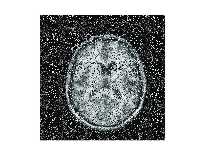
Fig. 2: Corrupted

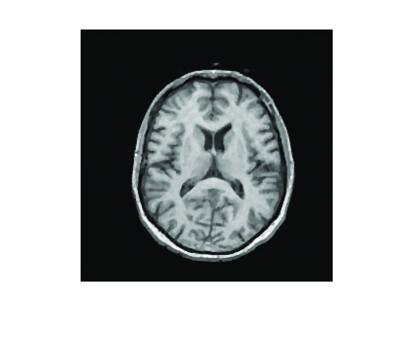
Fig. 3: $TV_{1}$ (SNR=19.21)

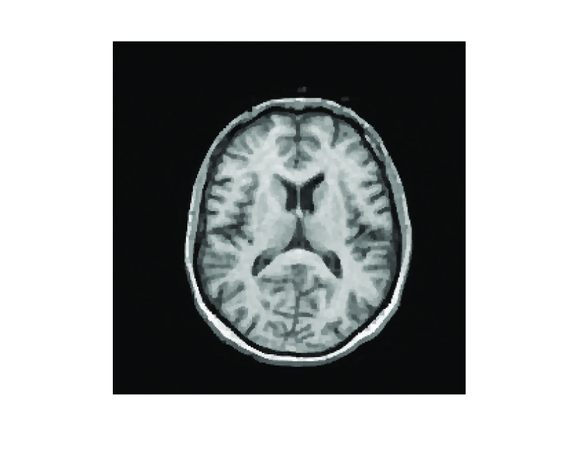
Fig. 4: $TV_{2}$ (SNR=17.66)

5.1 Example 2

This example illustrates the performance of TV/L1 algorithm when applied to the restoration of 3-channel RGB color images that have been contaminated by blur and salt and peppers noise. The corrupted image is stored in a block vector $B$ with three columns. The desired (and assumed unavailable) image is stored in the block vector $\widehat{X}$ with three columns. The blur-contaminated, and noisy image associated with $\widehat{X}$, is stored in the block vector $B$.

We consider the within-channel blurring only. Hence the blurring matrix $H_{1}$ in (1) is the $3\times 3$ identity matrix. The blurring matrix $H_{2}$ in (1), which describes the blurring within each channel, models Gaussian blur and is determined with the MATLAB function blur from [12]. This function has two parameters, the half-bandwidth of the Toeplitz blocks $r$ and the variance $\sigma$ of the Gaussian PSF. For this example we let $\sigma=1$ and $r=4$. The original (unknown) RGB image $\widehat{X}\in 256\times 256\times 3$ is the $\tt papav256$ image from MATLAB. It is shown in Figure 5. The associated blurred and noisy image $B$ with $30\%$ noise level is shown in Figure 6. Given the contaminated image $B$, we would like to recover an approximation of the original image $\widehat{X}$. The recovery of the image via $TV_{1}/L1$ and $TV_{2}/L1$ models is terminated as soon as $\left\|X_{k+1}-X_{k}\right\|_{F}/\left\|X_{k}\right\|_{F}<10^{-2}.$ Table 2 compares the results obtained by $TV_{1}/L1$ and $TV_{2}/L1$ models.

The restorations obtained with $TV_{1}/L1$ and $TV_{2}/L1$ for noise level $30\%$ are shown in Figure 7 and the Figure 8, respectively.

	Parameters			$\text{TV}_{1}$			$\text{TV}_{2}$
Noise %	$\mu$	$\beta$	$\rho$	Iter	SNR	time	Iter	SNR	time
10	0.1	80	5	13	24.66	9.01	14	24.32	9.73
20	0.125	80	5	17	23.00	12.64	17	22.71	12.36
30	0.125	80	5	19	20.90	13.35	19	21.13	13.89

Table 2: Comparison of $TV_{1}/L1$ and $TV_{2}/L1$

models for the restoration of papav256.png test colour image corrupted by Gaussian blur and different salt-and-pepper noise.

Fig. 5: Original image

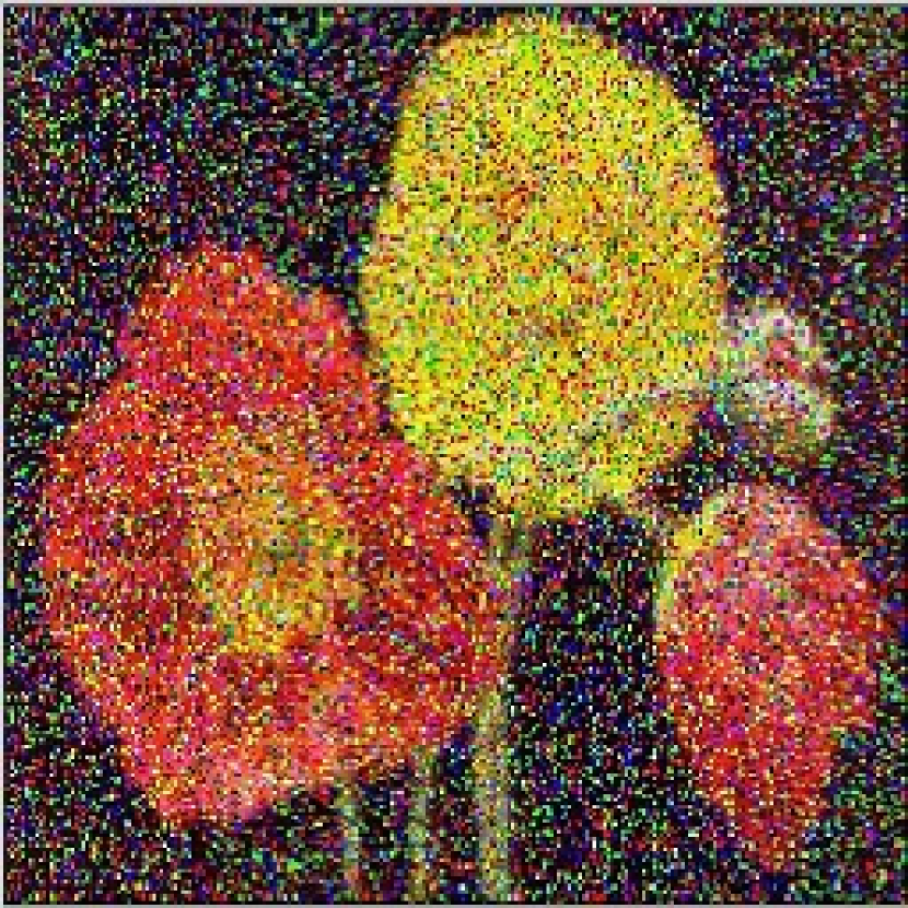
Fig. 6: Corrupted

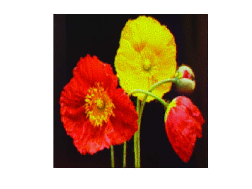
Fig. 7: $TV_{1}$ (SNR=20.90)

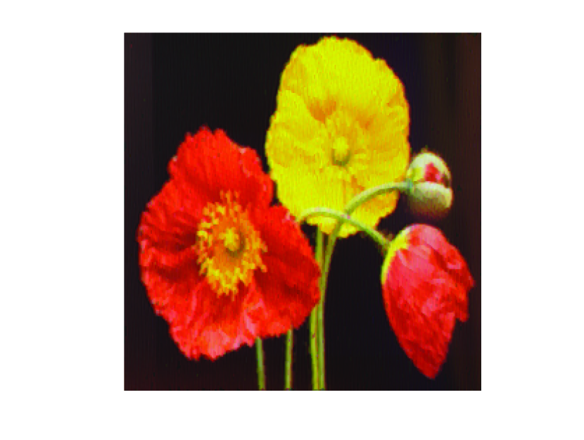
Fig. 8: $TV_{2}$ (SNR=21.13)

5.2 Example 3

In this example we present the experimental results recovered by Algorithm 1 for the reconstruction of a cross-channel blurred image. We consider the same original RGB image and the same within-channel blurring matrix $H_{1}$, as in Example 2, with the same parameters. The cross-channel blurring is determined by a matrix $H_{2}$. In our example we let $H_{2}$ to be

$$H_{2}=\begin{bmatrix}0.7&0.2&0.1\\ 0.25&0.5&0.25\\ 0.15&0.1&0.75\end{bmatrix}.$$

This matrix is obtained from [15]. The cross-channel blurred image without noise is represented by $H_{1}\widehat{X}H_{2}^{T}$ and it is shown in Figure (9) . The associated blurred and noisy image $B$ with $30\%$ noise level is shown in Figure (10). The cross-channel blurred and noisy image has been reconstructed using Algorithm 1 as soon as $\left\|X_{k+1}-X_{k}\right\|_{F}/\left\|X_{k}\right\|_{F}<10^{-2}.$ The restored images obtained with TV/L1 models are shown in Figures (12)-(11).

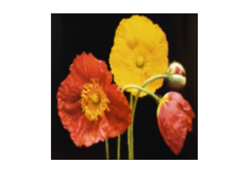
Fig. 9: Blurred image

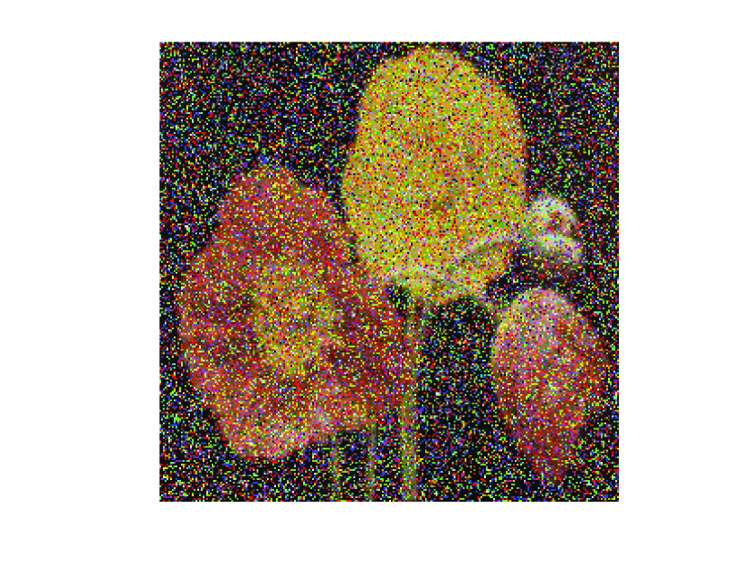
Fig. 10: Blurred and noisy image

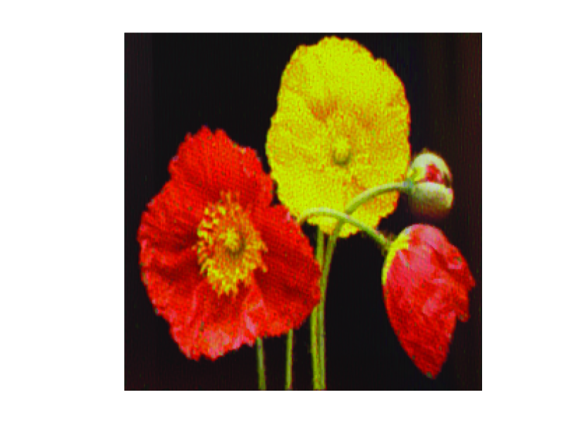
Fig. 11: $TV_{1}$ (SNR=19.50)

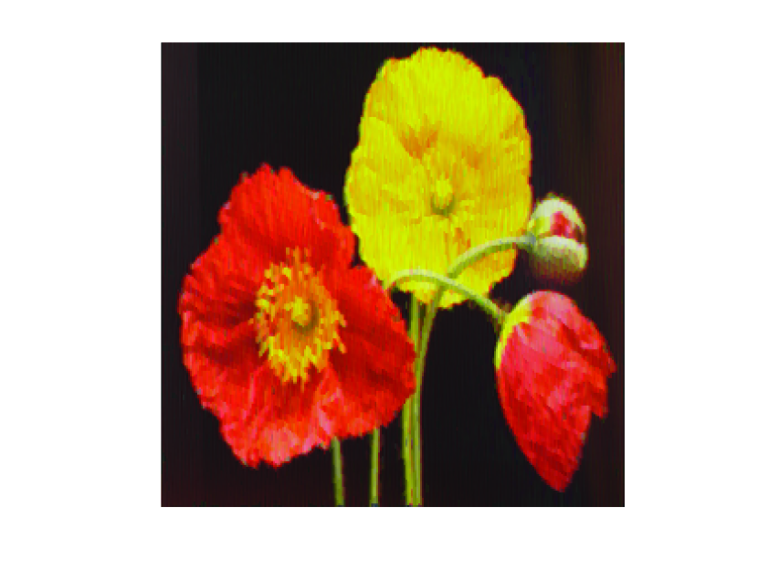
Fig. 12: $TV_{2}$ (SNR=19.90)

5.3 Example 4

In this example we consider the restoration of the gray-scale mrin6.png image degraded by the same blurring matrices $H_{1}$ and $H_{2}$ defined in Example 1 with $\sigma=2$ and $r=4$, and by additive zero-mean white Gaussian noise with different different noise levels. This noise level is defined as follows $\nu=\frac{||E||_{F}}{||\widehat{B}||_{F}}$, where $E$ denotes the block vector that represents the noise in $B$, i.e., $B:=\widehat{B}+E$, and $\widehat{B}$ is the noise-free image associated with original image $\widehat{X}$. For this kind of noise, we consider the $TV_{1}/L2$ and $TV_{2}/L2$ models. The recovery of the image via $TV_{1}/L1$ and $TV_{2}/L1$ models is terminated as soon as $\left\|X_{k+1}-X_{k}\right\|_{F}/\left\|X_{k}\right\|_{F}<10^{-3}.$ In Table 3, we compare the results obtained by $TV_{1}/L2$ and $TV_{2}/L2$ for different noise levels. Figure 14 shows the image degraded by $0.01$ noise level. Figure 15 and Figure 16 show the restored images obtained by $TV_{1}/L2$ and $TV_{2}/L2$, respectively.

	Parameters		$\text{TV}_{1}$			$\text{TV}_{2}$
Noise %	$\mu$	$\beta$	Iter	SNR	time	Iter	SNR	time
0.001	0.0001	0.1	53	18.32	9.30	52	18.32	10.10
0.01	0.001	30	20	15.70	2.65	21	15.60	2.60

Table 3: Comparison of $TV_{1}/L2$ and $TV_{2}/L2$

models for the restoration of imrin6.png test image corrupted by Gaussian blur and different white Gaussian noise level.

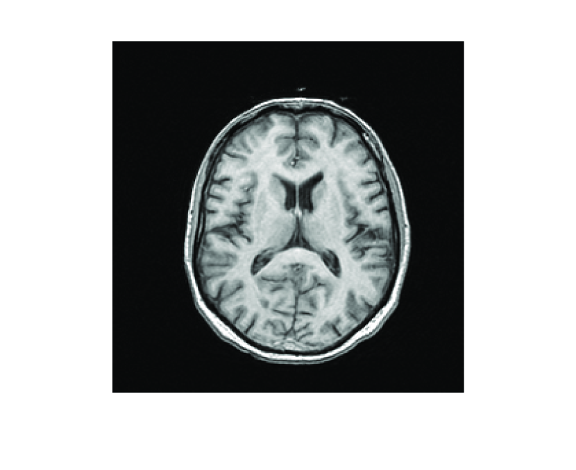
Fig. 13: Original image

Fig. 14: Corrupted

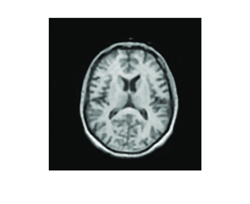
Fig. 15: $TV_{1}$ (SNR=15.70)

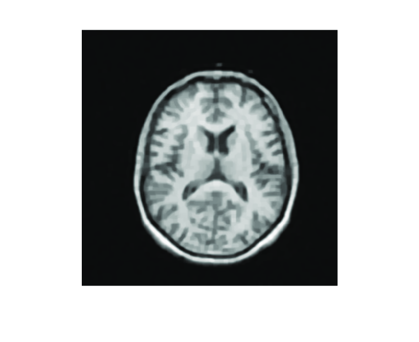
Fig. 16: $TV_{2}$ (SNR=15.60)

5.4 Example 5

In this example, we consider the Fredholm integral equation

$$\int\int_{\Omega}K(x,y,s,t)f(s,t)dsdt=g(x,y),\qquad(x,y)\in\Omega,$$ (114)

where $\Omega=[-6,6]\times[-6,6]$. Its kernel, solution, and right-hand side are given by

$$K(x,y,s,t)=k_{1}(x,s)k_{1}(y,t),\quad(x,y)\in\Omega,\quad(s,t)\in\Omega,$$

$$f(x,y)=f_{1}(x)f_{1}(y),$$

$$g(x,y)=g_{1}(x)g_{1}(y),$$

where

$$f_{1}(s):=\left\{\begin{array}[]{cl}1+\cos(\frac{\pi}{3}s),&\quad|s|\leq\frac{\pi}{3},\\ 0,&\quad\text{otherwise}.\end{array}\right.$$

$$k_{1}(s,x):=f_{1}(s-x)$$

$$g_{1}(s):=(6-|s|)\left(1+\frac{1}{2}\cos\left(\frac{\pi}{3}s\right)\right)+\frac{9}{2\pi}\sin\left(\frac{\pi}{3}|s|\right).$$

We use the code phillips from Regularization Tools [12] to discretize (114) by a Galerkin method with orthonormal box functions as test and trial functions to obtain $H_{1}$ and $H_{2}$ of size $500$. From the output of the code phillips we determine a scaled approximation $\widehat{X}\in\mathbb{R}^{500\times 500}$ of the exact solution $f(x,y)$. Figure 17 displays this exact solution. To determine the effectiveness of our approach, we evaluate the relative error

$$\text{Re}=\frac{||\widehat{X}-X_{k}||_{F}}{||\widehat{X}||_{F}}$$

of the computed approximate solution $X_{k}$ obtained with Algorithm 1. Table 4 shows the relative error in approximate solutions determined by Algorithm 1 for different noise levels, as well as the number of iterations required to satisfy $\left\|X_{k+1}-X_{k}\right\|_{F}/\left\|X_{k}\right\|_{F}<10^{-3}.$ Figure 18 displays the computed approximate solution obtained when the noise level is $0.1$.

	Parameters		$\text{TV}_{1}$			$\text{TV}_{2}$
Noise %	$\mu$	$\beta$	Iter	Re	time	Iter	Re	time
0.001	0.0001	0.1	12	$4.01\times 10^{-2}$	9.05	9	$4.71\times 10^{-2}$	6.52
0.01	0.001	30	13	$3.99\times 10^{-2}$	9.63	13	$3.98\times 10^{-2}$	9.66
0.1	0.1	40	15	$4.07\times 10^{-2}$	10.94	15	$4.07\times 10^{-2}$	11.38

Table 4: Comparison of $TV_{1}/L2$ and $TV_{2}/L2$

models for the solution of (114) with different white Gaussian noise level.

Fig. 17: True object

Fig. 18: Approximate solution

References

- [1] H. Andrews and B. Hunt, Digital Image Restoration, Prentice-Hall, Engelwood Cliffs, 1977.
- [2] M. Bertero and P. Boccacci, Introduction to Inverse Problems in Imaging, IOP Publishing, London, 1998.
- [3] A. Bouhamidi and K. Jbilou, A note on the numerical approximate solution for generalized Sylvester Matrix equations, Appl. Math. Comput., 206(2)(2008) 687–694.
- [4] R. Bouyouli, K. Jbilou, R. Sadaka and H. Sadok, Convergence properties of some block Krylov subspace methods for multiple linear systems. J. Comput. Appl. Math., 196 (2006) 498–511.
- [5] S. Boyd, N. Parikh, E. Chu, B. Peleato, and J. Eckstein. Distributed optimization and statistical learning via the alternating direction method of multipliers. Foundations and Trends in Machine Learning, 3(1):1–122, 2011.
- [6] B. Chalmond, Modeling and Inverse Problems in Image Analysis, Springer, New York, 2003.
- [7] F. Facchinei and J.S. Pang, Finite-dimensional variational inequalities and complementarity problems, Springer Series in Operations Research, Springer-Verlag, Berlin, 2003.
- [8] D. Gabay and B. Mercier,A dual algorithm for the solution of nonlinear variational problems via finite-element approximations, Comput. Math. Appl., 2 (1976) 17–40.
- [9] T. Goldstein and S. Osher, The split Bregman L1 regularized problems,” SIAM J. Imaging Sci., 2, pp. 323-343, 2009.
- [10] R. Glowinski, Numerical Methods for Nonlinear Variational Problems. Springer Verlag, 2008
- [11] N. P. Galatsanos, A. K. Katsaggelos, R. T. Chin, AND A. D. Hillary, Least squares restoration of multichannel images, IEEE Trans. Signal Proc., 39 (1991) 2222–2236.
- [12] P. C. Hansen, Regularization tools version 4.0 for MATLAB 7.3, Numer. Algorithms, 46 (2007), pp. 189–194.
- [13] M. R. Hestenes, Multiplier and gradient methods, Journal of Optimization Theory and Applications, 4 303–320, and in Computing Methods in Optimization Problems, 2 (Eds L.A. Zadeh, L.W. Neustadt, and A.V. Balakrishnan), Academic Press, New York, 1969.
- [14] B. He, L. Liao, D. Han and H. Yang, A new inexact alternating directions method for monotone variational inequalities, Math. Program., 92(1) (2002), pp. 103–118.
- [15] P. C. Hansen, J. G. Nagy, and D. P. O’Leary, Deblurring Images: Matrices, Spectra, and Filtering, SIAM, Philadelphi, 2006.
- [16] A. K. Jain, Fundamentals of Digital Image Processing, Prentice-Hall, Engelwood Cliffs, 1989.
- [17] K. Jbilou, A. Messaoudi and H. Sadok, Global FOM and GMRES algorithms for matrix equations, Appl. Numer. Math, 31(1999) 49–63.
- [18] C. Li, An Efficient Algorithm For Total Variation Regularization with Applications to the Single Pixel Camera and Compressive Sensing, Ph.D. thesis, Rice University, 2009, available at http://www.caam.rice.edu/ ∼optimization/L1/TVAL3/tval3 thesis.pdf
- [19] A. Lanza, S. Morigi, L. Reichel, and F. Sgallari, A generalized Krylov subspace method for minimization. SIAM J. Sci. Comput. 37(5), S30–S50 (2015)
- [20] F. Li, M. K. Ng, AND R. J. Plemmons, Coupled segmentation and denoising/deblurring for hyperspectral material identification, Numer. Linear Algebra Appl., 19 (2012) 15–17
- [21] J. Lampe, L. Reichel, and H. Voss , Large-scale Tikhonov regularization via reduction by orthogonal projection, Linear Algebra Appl., 436 (2012) 2845–2865.
- [22] M. J. D. Powell, A method for nonlinear constraints in minimization problems, Optimization (Ed. R. Fletcher), Academic Press, London, New York, (1969) 283– 298.
- [23] L. Rudin, S. Osher, and E. Fatemi, Nonlinear total variation based noise removal algorithms, Physica D. 60 1992 259-2680
- [24] R.T. Rockafellar, Convex Analysis, Princeton University Press, Princeton, NJ, 1970
- [25] C. R. Vogel, Computational Methods for Inverse Problems, SIAM, Philadelphia, PA, 2002.
- [26] C. R. Vogel and M. E. Oman, Fast, robust total variation-based reconstruction of noisy blurred images, IEEE Trans. Image Proc., 7, pp. 813-824, 1998.
- [27] A. Tikhonov, and V. Arsenin, Solution of ill-posed problems, Winston, Washington, DC, 1977.
- [28] S. J. Wright, M. A. T. Figueiredo, and R. D. Nowak, Sparse Reconstruction by Separable Approximation, IEEE Trans. Signal Processing, 57(7):2479–2493, 2009.
- [29] C. L. Wu, J. Y. Zhang, and X. C. Tai, Augmented Lagrangian method for total variation restoration with non-quadratic fidelity, Inverse Problems and Imaging, 5, pp. 237-261, 2010.