Real-time evolution method and its application to 3 cluster system
Abstract
A new theoretical method is proposed to describe the ground and excited cluster states of atomic nuclei. The method utilizes the equation-of-motion of the Gaussian wave packets to generate the basis wave functions having various cluster configurations. The generated basis wave functions are superposed to diagonalize the Hamiltonian. In other words, this method uses the real time as the generator coordinate. The application to the system as a benchmark shows that the new method works efficiently and yields the result consistent with or better than the other cluster models. Brief discussion on the structure of the excited and states is also made.
pacs:
Valid PACS appear hereI Introduction
It has long been known that the Hoyle state (the state of ) is a dilute gas-like cluster state dominated by the -wave Uegaki et al. (1978); Fujiwara et al. (1980); Kamimura (1981); Descouvemont and Baye (1987); Kanada-En’yo (1998); Descouvemont et al. (2003); Chernykh et al. (2007); Kanada-En’yo (2007a). Later, it was pointed out that the Hoyle state can be regarded as a Bose-Einstein condensate of particles Tohsaki et al. (2001); Yamada et al. (2012); Schuck et al. (2016). This findings motivated many studies on and the related topics. For example, the idea of the particle condensate has been extended to other excited states above the Hoyle state. Namely, the state at 10.03 MeV Freer et al. (2009); Itoh et al. (2011); Zimmerman et al. (2011, 2013) and the state at 13.3 MeV Freer et al. (2011) are considered as the members of the ”Hoyle band” Freer and Fynbo (2014); Funaki (2015); Schuck et al. (2016). More recently, the state at 10.3 MeV Itoh et al. (2011, 2013) is suggested as the ”breathing mode” of the Hoyle state Kurokawa and Kato (2005, 2007); Ohtsubo et al. (2013); Funaki (2015, 2016); Zhou et al. (2016). The possible formation of the 3 linear-chain ( state) has also been discussed Funaki (2015, 2016).
The discussion has been naturally extended to the condensate of many particles. The candidates of the 4 condensate in are under the intensive discussions Wakasa et al. (2007); Funaki et al. (2008); Curtis et al. (2013); Rodrigues et al. (2014); Bijker and Iachello (2014); Ogloblin et al. (2016); Bijker and Iachello (2017); Li et al. (2017a). However, the theoretical and experimental information for the 5 and more particle condensate Yamada and Schuck (2004); Kokalova et al. (2006); Itagaki et al. (2007); Schuck et al. (2016) is rather scarce. The clustering of non- nuclei is another direction of the extension. For example, the Hoyle-analog states with a nucleon hole or particle are discussed for Descouvemont (1995); Kanada-En’yo (2007b); Kawabata et al. (2007); Yamada and Funaki (2010) and Yamada et al. (2006); Yamada and Funaki (2015). The 3 linear-chains accompanied by the valence neutrons are expected in neutron-rich C isotopes Itagaki et al. (2001); Suhara and Kanada-En’yo (2010); Freer et al. (2014); Baba et al. (2014); Ebran et al. (2014); Dell’Aquila et al. (2016); Fritsch et al. (2016); Tian et al. (2016); Baba and Kimura (2016); Li et al. (2017b); Yamaguchi et al. (2017); Baba and Kimura (2017). Thus, nowadays the researches are extending to the highly excited cluster states composed of many clusters and nucleons.
However, when the number of the constituent clusters or nucleons increases, the description of the cluster states becomes difficult. For example, suppose that one employs the generator coordinate method (GCM) Hill and Wheeler (1953); Griffin and Wheeler (1957) which superposes many basis wave functions. Then, it is easy to imagine that the number of basis wave functions required for the description of the cluster states increases very quickly as the number of constituent particles increases or the system becomes dilute. As a result, much computational power is demanded and the practical calculation becomes difficult. This may be one of the reason why the 5 and more particle condensate are rarely studied based on the microscopic models. Therefore, new method which efficiently generates the basis wave functions is highly desirable and indispensable. For this purpose, several methods have been developed such as the stochastic sampling of the basis wave functions Suzuki and Varga (1998); Itagaki et al. (2003); Mitroy et al. (2013) and the imaginary-time development method Fukuoka et al. (2013).
In this study, we propose an alternative method which utilizes the equation-of-motion (EOM) of the Gaussian wave packets. The basis wave functions are generated by the real-time evolution of the system governed by the EOM, and they are superposed to diagonalize the Hamiltonian. In other words, this method employs the real time as the generator coordinate. As a benchmark of the methodology, we applied it to the system (). It is shown that the new method works efficiently and yields the result consistent with or better than the other cluster models. Furthermore, based on the isoscalar (IS) monopole and dipole transition strengths, we briefly discuss the structure of the excited and states.
This paper is organized as follows. In the next section, we explain the framework of the new method named real-time evolution method (REM). In the section III, we present the result of the numerical benchmark. We also discuss the structure of the excited and states briefly. The final section summarizes this work.
II Theoretical framework
Here, we explain the framework of the real-time evolution method. For simplicity, we assume its application to the cluster wave functions ( nuclei). However, it is noted that the method is also applicable to more general cases such as non- cluster wave functions, antisymmetrized molecular dynamics (AMD) and fermionic molecular dynamics (FMD) wave functions.
II.1 Hamiltonian and GCM wave function
The Hamiltonian for the systems composed of 4 nucleons is given as,
| (1) |
where and respectively denote the kinetic energies of the nucleons and the center-of-mass. The and denote the effective nucleon-nucleon interaction and Coulomb interactions, respectively. The parameter set of is explained later.
As for the intrinsic wave function of system, we employ the Brink-Bloch wave function Brink (1966) which is composed of clusters having configurations,
| (2) | |||
| (3) | |||
| (4) |
Here denotes the wave packet describing the cluster located at . The three-dimensional vectors are complex numbered and describe the cluster positions in the phase space.
Similarly to other cluster models, we superpose the intrinsic wave function having different configurations (different sets of the complex vectors ) after the parity and angular momentum projection (GCM). The most general form of the GCM wave function may be written as,
| (5) |
where is the parity and angular momentum projector. The amplitude of the superposition must be determined in some ways. For example, the original THSR wave function () Tohsaki et al. (2001) asserts that the amplitude can be written as
| (6) |
where the vectors are reduced to the real valued vectors , and the parameter controls the size of the particle condensate. It is known that this THSR ansatz works surprisingly well for the ground and excited states of Tohsaki et al. (2001); Funaki et al. (2003); Yamada et al. (2012); Schuck et al. (2016).
In other ordinary cluster models, Eq. (5) is often discretized and approximated by a sum of the finite number of the basis wave functions,
| (7) |
and the amplitude is calculated by the Griffin-Hill-Wheeler equation Hill and Wheeler (1953); Griffin and Wheeler (1957). Here, denotes the th set of the vectors and the number of the superposed basis wave function is equal to . If is sufficiently large and the set of the vectors covers various configurations of clusters, Eq. (7) will be a good approximation, but the increase of requires much computational cost. It is easy to imagine that the number of basis wave function required for a reasonable description of systems will be greatly increased, when the number of particle is increased. This is one of the reason, for example, why the condensation of 5 and more particles are rarely studied by the microscopic models.
Therefore, if one employs the approximation given by Eq. (7), it is essentially important to find a method which efficiently generates the set of the vectors to reduce the computational cost. For this purpose, several methods such as the stochastic method Suzuki and Varga (1998); Itagaki et al. (2003); Mitroy et al. (2013) and the imaginary time evolution methods Fukuoka et al. (2013) have been proposed, and in this study, we introduce a new method which uses the real-time evolution of the particle wave packets.
II.2 Real-time evolution method
In the present study, the EOM of the particle wave packets is used to generate the sets of the vectors . By applying the time-dependent variational principle to the intrinsic wave function given by Eq. (2),
| (8) |
one obtains the EOM for the particle centroids ,
| (9) | |||
| (10) | |||
| (11) |
Starting from an arbitrary initial wave function at , we solve the time evolution of . As a result, the EOS yields the set of the vectors as function of the time , which defines the wave function at each time. Despite of its classical form, this EOM still holds the information of the quantum system. For example, it was shown that the nuclear phase shift of the - scattering can be obtained from the classical trajectory of the wave packet centroids Saraceno et al. (1983). In addition to this, it was shown that the ensemble of the wave functions possesses following good properties Schnack and Feldmeier (1996); Ono and Horiuchi (1996a, b).
-
1.
The ensemble of the time-dependent wave functions has ergodic nature
-
2.
And it follows the quantum statistics
if the nucleon-nucleon collisions and nucleon emission processes are properly treated. Indeed, on the basis of this EOM properties, the nuclear liquid-gas phase transition during the heavy-ion collisions and the caloric curve for the finite nuclei have been studied Schnack and Feldmeier (1997); Sugawa and Horiuchi (1999); Furuta and Ono (2006); Kanada-En’yo et al. (2012). Therefore, we expect that, if time is evolved long enough, the ensemble of the wave functions spans a good model space for systems. In other words, we expect that the bound and resonant states of systems are reasonably described by the superposition of the basis wave functions as follows,
| (12) |
Here, the complex conjugated basis wave functions are also superposed to properly describe time-even states. The coefficients and should be determined by the diagonalization of the Hamiltonian. Eq. (12) can be regarded as the GCM wave function which employs the real-time as the generator coordinate.
II.3 Numerical calculation
In this study, REM calculation is performed for cluster system (). For the sake of the comparison, we used the Volkov No. 2 effective nucleon-nucleon interaction Volkov (1965) with a slight modification Fujiwara et al. (1980); Kamimura (1981), which is common to the other studies using resonating group method (RGM) Fujiwara et al. (1980); Kamimura (1981) and Tohsaki-Horiuchi-Schuck-Röpke (THSR) wave function Funaki et al. (2003); Funaki (2015, 2016). The numerical calculation was performed in the following steps.
(1) In the first step, we randomly generate cluster wave function and calculate the imaginary-time evolution of the system,
| (13) |
where is an arbitrary negative number. Eq. (13) decreases the intrinsic energy , as the imaginary time is evolved. The imaginary-time evolution is continued until the intrinsic excitation energy,
| (14) |
equals to a certain value. Here, is the minimum intrinsic energy obtained by the very long imaginary-time evolution, which is -74.5 MeV in the present Hamiltonian. In the practical calculation, we tested several values of (10, 20, 25 and 30 MeV) and found that MeV results in the best convergence.
(2) In the second step, we calculate the real-time evolution (Eq. (9)) starting from the initial wave function obtained in the first step. For the numerical calculation, the time is discretized with an interval of fm/c,
| (15) |
and the maximal propagation time is fm/c. It is noted that the intrinsic energy , and hence , is conserved by the EOM. As a result, the time evolution calculation yields a set of the Brink-Bloch wave functions having the same . And it is used as the basis wave function of the GCM calculation in the next step.
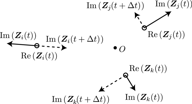
If is large, clusters occasionally escape out to infinite distance during the time evolution. This yields basis wave functions having unphysically large radius, which are useless for the description of the bound or resonant states. To avoid this problem, we impose additional condition to the calculation. When the condition,
| (16) |
is satisfied, i.e. if any of clusters is distant more than , we interchange their momentum by hand as follows,
| (17) | ||||
| (18) | ||||
| (19) |
where we assume that . It is noted that the real part of corresponds the coordinate of cluster, while the imaginary part corresponds to the momentum. As a result, clusters rebound as illustrated in Fig. 1. In the present calculation, the maximum distance is chosen as fm.
(3) Thus-obtained basis wave functions are superposed by using the real-time as a generator coordinate. In the following we call this step GCM calculation. Since the time is discretized, Eq. (12) should read,
| (20) |
Here, the basis wave function is abbreviated as . The set of the coefficient , and the eigen-energy are determined by solving the Griffin-Hill-Wheeler equation to diagonalize the Hamiltonian.
In the practical calculation, a set of basis wave functions obtained by the time evolution is severely redundant. This makes it difficult to solve the Griffin-Hill-Wheeler equation accurately. To avoid this problem, we remove the basis wave functions which have large overlap with others. When a basis wave function satisfies the following condition,
| (21) |
it is removed from the ensemble. Namely, we do not use the basis wave functions which have the overlap with the past wave functions larger than . In the present calculation is chosen as 0.75.
(4) As discussed later, above-explained GCM calculation has problem to describe highly excited broad resonances, because of contamination of the non-resonant wave functions. To overcome this problem, we apply the -constraint method proposed by Funaki et al. Funaki et al. (2006). Following this method, we first diagonalize the radius operator,
| (22) | |||
| (23) |
which defines a new set of the basis wave functions,
| (24) |
corresponding to the eigenvalue . Superposing these new basis, we construct the -constrained GCM wave function,
| (25) |
Here denotes the conditional summation running over all which satisfy the condition . Namely, the basis wave functions which have too large eigenvalue of the radius operator are excluded. The coefficients , and the eigen-energies are determined by solving the Griffin-Hill-Wheeler equation. It has been shown that this method effectively separates the resonant states from the non-resonant states. In the present calculation, the cut-off radius is varied ranging from to to check the convergence.
III Numerical Results
In this section, we explain how our method works, and compare the obtained result with those of other models to check the validity and efficiency of the REM. The detailed discussion on the structures of cluster states in will be made in our forthcoming work.
III.1 Real-time evolution
As explained in the previous section, the REM relies on the ergotic nature of the EOM. Therefore, if the time is propagated long enough, the results should be converged and should not depend on the initial wave functions. To check these points, we tested two different initial wave functions with MeV to yield ensembles of the wave functions, which we denote set 1 and 2.
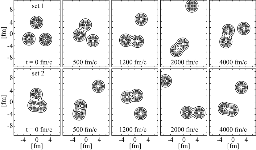
To illustrate how the 3 system is evolved by the EOM, Fig. 2 shows the several wave functions of set 1 and 2 at particular times. In both ensembles, disregard to the initial condition, clusters distribute in various ways; they are close to each other in some time and far distant in another time. Actually, the system repeats spatial expansion and contraction as time being evolved, which can be confirmed from the radius of the system as function of time shown in Fig. 3 (a). It is noted that the unphysical change of the expansion velocity at the maximum radius around 9 fm is because of the artificial rebound of the clusters described by Eqs. (17)-(19).
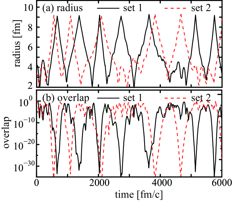
Figure 3 (b) shows the squared overlap between the wave function and initial wave function after the projection to state, that is defined as,
| (26) |
We see that the overlap is rather small, and hence, the wave function is almost orthogonal to the initial wave function in most of the time. Thus, the EOM generates various cluster configurations automatically.
III.2 Convergence without and with -constraint
We first discuss the GCM results obtained without -constraint. Figure 4 shows the energies the states as functions of the maximum propagation time .
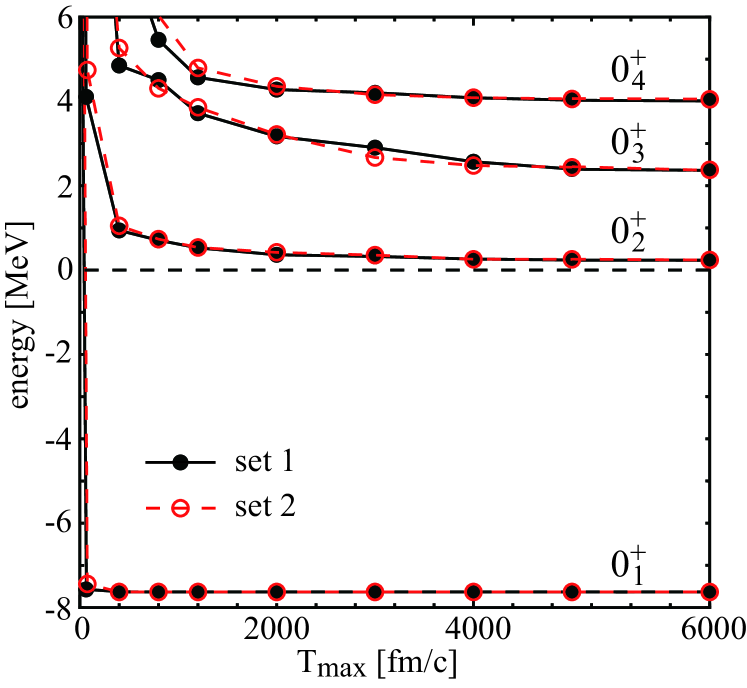
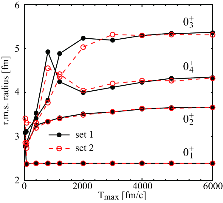
We see that the energies of the states converge and are independent of the initial wave functions, if the propagation time is long enough. In particular, the energy of the ground state converges very quickly, despite of the rather high intrinsic excitation energy ( MeV) of the basis wave functions generated by the EOM. We also found that the quick convergence is common to another bound state ( state).
On the other hand, the energy convergence of the excited states is not as fast as that of the ground state. In particular, it is interesting to note that the convergence of the state looks much slower than others. This is related to the fact that the state is a very broad resonance Itoh et al. (2011, 2013). Furthermore, if we observe the figure carefully, we find that the energies of these unbound states still go down even at large . This is because of the contamination of the non-resonant wave functions to these excited states, which can be seen more clearly in the dependence of the radius shown in Fig. 5. Again we see that the convergence of the ground state is surprisingly fast, but the unbound states are not. In this figure, we clearly observe that the radii of the unbound states continuously increases showing the contamination of non-resonant wave functions with huge radii.
To avoid the contamination of the non-resonant wave functions, we applied the -constraint Funaki et al. (2006). This prescription excludes the basis wave function with huge radius and makes it possible to obtain approximate energies and wave functions of the resonant states. Since the -constraint was already applied to THSR wave function Funaki (2015, 2015); Zhou et al. (2016), it is worthwhile to compare the results between THSR and REM with -constraint.
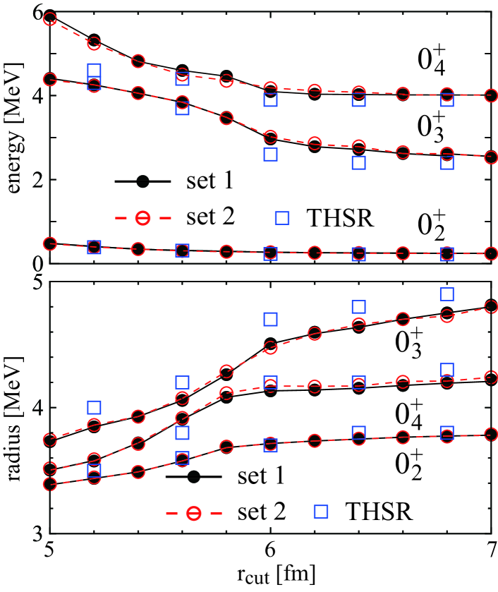
Figure 6 shows the energies and radii of the excited states obtained by the -constraint. The energies of the and states are approximately constant in the region of the fm, and the radii are very slowly increases as function of . This implies that the most of the resonant wave functions in the interaction region is already described by the basis wave functions with fm, and the choice of the fm will give reasonable approximation for the and states. We also note the results for the and look almost consistent with the THSR results. On the other hand, we have not obtained the reasonable convergence for the state. In particular, the radius continues to increase as function of not only in the REM calculation but also in the THSR calculation, which implies the contamination non-resonant wave functions. This requires more sophisticated method such as the complex scaling for more precise discussion of this state Kurokawa and Kato (2005, 2007); Ohtsubo et al. (2013).
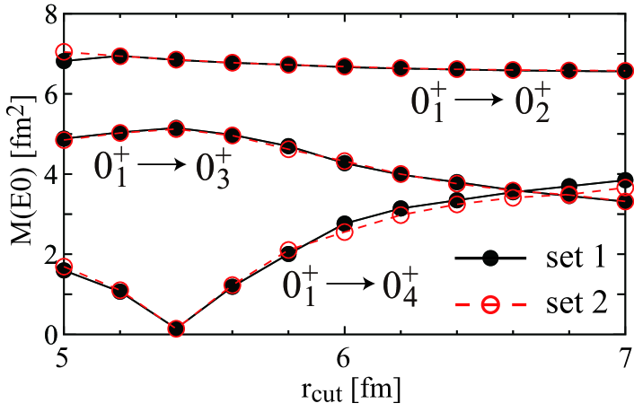
Finally, Fig. 7 shows the electric monopole transition matrix between the ground and excited states. Again we see that the Hoyle state is quite stable, while the and are dependent on . Since the monopole matrix element is very sensitive to the outer side of the wave functions, this behavior also indicates the non-negligible contamination of the continuum states with large radii.
III.3 Excitation spectrum of
Here, we discuss the excitation spectrum of and make brief comments on the structure of several states. Figure 8 shows the excitation spectrum of calculated by the REM with the ensemble set 1 and fm together with t hose by the RGM Fujiwara et al. (1980); Kamimura (1981) and THSR Funaki (2015, 2016). Their energies and radii are also listed in Tab. 1
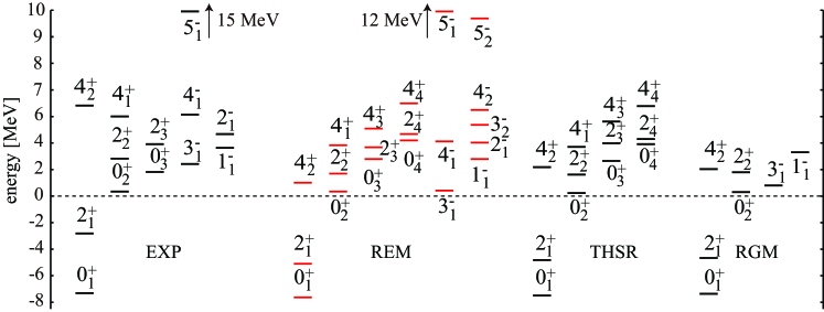
Note that all of these calculations use the same Hamiltonian, and hence, they should be consistent to each other and the deeper binding energy means a better wave function for the bound states. We see that all of the theoretical results are qualitatively consistent to each other. In particular, REM and THSR results are reasonably agree for all positive-parity states which include the compact shell-model-like ground band and highly-excited cluster states. As for the negative-parity states, REM and RGM reasonably agree for the and states, and REM additionally produces the , and states, which are also described by AMD Kanada-En’yo (1998, 2007a) and FMD Chernykh et al. (2007). In short, REM can describe all of the states reported by THSR and RGM reasonably. It must be emphasized that not only the states but all of the state shown in Fig. 8 were obtained from a single ensemble set 1, which means that the EOM really effectively generates the basis wave functions.
| REM | THSR Funaki (2015, 2016); Schuck et al. (2016) | RGM Fujiwara et al. (1980); Kamimura (1981) | EXP | |||||
|---|---|---|---|---|---|---|---|---|
| -7.6 | 2.4 | -7.5 | 2.4 | -7.4 | 2.4 | -7.3 | 2.4 | |
| -5.1 | 2.4 | -4.8 | 2.4 | -4.6 | 2.4 | -2.8 | ||
| 1.0 | 2.3 | 2.2 | 2.3 | 2.0 | 2.3 | 6.8 | ||
| 0.3 | 3.7 | 0.2 | 3.7 | 0.4 | 3.5 | 0.4 | ||
| 1.7 | 3.9 | 1.6 | 3.9 | 2.1 | 4.0 | 2.8 | ||
| 3.8 | 4.5 | 3.7 | 4.5 | 6.0 | ||||
| 2.8 | 4.6 | 2.7 | 4.7 | 1.8 | ||||
| 3.9 | 4.6 | 4.0 | 4.5 | 3.9 | ||||
| 5.4 | 4.8 | 5.6 | 4.7 | |||||
| 4.0 | 4.2 | 3.9 | 4.2 | |||||
| 4.6 | 3.7 | 4.3 | 4.1 | |||||
| 6.6 | 5.0 | 6.8 | 4.7 | |||||
| 0.4 | 2.8 | 0.8 | 2.8 | 2.4 | ||||
| 4.1 | 2.9 | 6.1 | ||||||
| 12 | 3.6 | 15 | ||||||
| 2.8 | 4.3 | 3.4 | 3.4 | 3.6 | ||||
| 4.0 | 3.5 | 4.6 | ||||||
| 5.4 | 4.5 | |||||||
| 6.4 | 4.7 | |||||||
| 9.3 | 4.5 | |||||||
Now, we discuss the details of the energies and radii listed in Tab. 1. Firstly, for many of the and states, we see that REM yields deeper binding energy than THSR and RGM. This may be due to the limitation of the model space of the THSR and RGM calculations. Namely, the THSR calculation assumes the axially symmetric intrinsic state and RGM calculation limits the relative angular momentum between clusters up to 2, while REM has no such assumptions. Secondly, THSR often yields smaller excitation energies and larger radii for highly excited states such as , and states. Although the variational principle cannot be applied to these highly excited broad resonances, the difference may be attributed to the difference in the long range part of the wave functions. THSR uses central Gaussians with large size parameters, while REM uses localized Gaussians with relatively smaller size parameters. Therefore, THSR should have better description for the long-range part of the dilute states.
We also comment the difference between the models. In the THSR calculation, the positive-parity condensate was assumed, hence the negative-parity is missing in the figure. However, if an extended version of THSR is applied, we expect that it yields the negative-parity states consistent with REM and RGM. In the RGM calculation, neither -constraint nor other techniques to eliminate the non-resonant state were applied. As a result, it cannot describe many highly excited states with large widths.
Finally, we discuss the characteristics of the excited and states referring their electric monopole and dipole transition strengths. The transition matrix are defined as,
| (27) | ||||
| (28) |
where denotes the single-particle coordinate measured from the center-of-mass. The results are summarized in Tab. 2.
| transition | REM | THSR Funaki (2015, 2016); Schuck et al. (2016) | RGM Fujiwara et al. (1980); Kamimura (1981) | EXP Strehl (1970) |
|---|---|---|---|---|
| 6.4 | 6.3 | 6.7 | ||
| 3.8 | 3.9 | |||
| 3.3 | 3.5 | |||
| 28 | 34 | |||
| 0.7 | 0.5 | |||
| 3.7 | ||||
| 45 |
Since the monopole transition operator is nothing but the radius operator, the matrix element should be large for the dilute gas-like states Yamada et al. (2008). Indeed, it is well known that the Hoyle state has the enhanced monopole transition strength from the ground state because of its dilute gas-like nature. The present calculation yields 6.4 (1.5 WU) which is consistent with the other cluster models, but slightly overestimates the observation. The monopole transition from the ground state to the more dilute state is also large and comparable with the Weisskopf unit (WU), but not as large as that of the Hoyle state. The reason of the reduction is that the state is dominantly composed of the configurations which cannot be excited by the monopole operator ( excitation). However, it must be noted that the transition from the Hoyle state to the state is greatly enhanced (6.2 WU). From this result and from the analysis of the wave function, it was concluded that the state is a excited state built on the Hoyle state Funaki (2015, 2016). In other words, it is the breathing mode of the Hoyle state Zhou et al. (2016). This relationship between the ground, Hoyle and states are schematically illustrated in Fig. 9. On the contrary, the monopole transition between the Hoyle state and the state is rather weak. This is due to the structural mismatch between these states. In Ref. Funaki (2016), it was concluded that the clusters are linearly aligned in the state (linear-chain state), which naturally reduces the overlap with the Hoyle state.
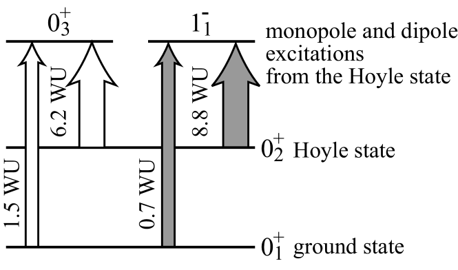
A new finding in the present study is that not only the state but also the state may be an excited state of the Hoyle state. As discussed in Ref. Chiba et al. (2016), the states with pronounced clustering should have the strong IS dipole transition strength from the ground state. The present calculation yields which is comparable with the Weisskopf unit (0.7 WU). A similar strength was also obtained by the AMD calculation Kanada-En’yo (2016). Furthermore, it must be noted that the IS dipole transition between the Hoyle state and the state is extraordinary strong (8.8 WU). From this result, we are tempted to conclude that the state is the (or ) excitation of the Hoyle state. Indeed the state has huge radius comparable with the state. It is also interesting to note that the state is energetically very close to the state. This conjecture is also illustrated in Fig. 9.
To discuss the similarity between the and states in a different way, we optimized a single Brink-Bloch wave function (optimized the position of 3 clusters) so that the overlap with the REM wave functions is maximized. Here the overlap is defined as,
| (29) |
where denotes the REM wave function for the and states and is a Brink-Bloch wave function to be optimized. Thus-obtained optimized Brink-Bloch wave functions shown in Fig. 10 tell us the most likelihood cluster configuration for each state.
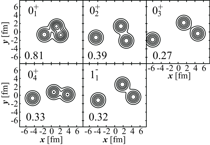
It can be seen that the ground state is represented by a Brink-Bloch wave function with short inter-cluster distances whose overlap amounts to 0.81. This is due to the dominance of the configuration which can be described by a single Brink-Bloch wave function. On the contrary, the most liklihood cluster configuration of the Hoyle state has large inter-cluster distance and it only explains about 39% of the Hoyle state. Indeed, not only the configuration shown in Fig. 10, but many other configurations also have the overlaps of the same magnitude. This indicates that the Hoyle state is not a single cluster configuration but a superposition of many different configurations, which is consistent with the dilute nature of the Hoyle state. The dilute character can be more strongly seen in the and states. The likelihood configurations of these states have the inter-cluster distances larger than the Hoyle state, and the overlaps are rather small. Thus, we expect that the state can be also regarded as the family of the Hoyle state. We also comment that the state does not look a perfect linear-chain configuration, but has a bent-armed configuration. The smallness of the overlap may mean that this state is not stable against the bending motion. This interpretation is consistent with the discussion made in Refs. Itagaki et al. (2001); Kanada-En’yo (2007a); Funaki (2016). We also note that this cluster configuration is more or less similar to the bent-armed cluster configuration of the Hoyle state suggested by the Lattice calculation Epelbaum et al. (2012).
IV Summary
In summary, we have developed a new theoretical model which utilizes the classical EOM of the Gaussian centroids to generate the ergodic ensemble of the basis wave functions. The generated basis wave functions are superposed to diagonalize the Hamiltonian. Thus, the method named REM can be regarded a generator coordinate method which employs the real time as the generator coordinate.
As a benchmark of REM, we applied it to the 3 system () and found that the result is consistent with or even better than the other cluster models. It was shown that when the propagation time is long enough the energies and radii of the ground and many excited states are converged and independent of the initial condition. As a result, REM successfully described all of the states reported by THSR and RGM. It must be emphasized that all the states are obtained from a single ensemble of the basis wave function, which indicates that the EOM effectively generates the basis wave functions. However, even if we apply the -constraint, several excited states were not converged well because of the contamination of the non-resonant wave function. Particular case is the state which has broad width and is regarded as the breathing mode of the Hoyle state. More accurate description of these states requires further development of the method.
Based on the isoscalar monopole and dipole transition strengths, the characteristics of the excited and states are discussed. We confirmed that the properties of the Hoyle state and the states are consistent with those discussed in the preceding studies. They have dilute structure and the enhanced monopole transition strengths from the ground state. The huge monopole transition strength between the Hoyle state and the state was also confirmed. In addition to this, we found that the state has the analogous properties to the state. Namely, the state has dilute structure and the enhanced dipole transition strengths from the ground state. It also has the extraordinary large IS dipole strength from the Hoyle state. From these results, we conjecture that the state can be also regarded as an excitation mode of the Hoyle state. Although this conjecture is based on only the transition strengths and the overlaps, more detailed quantitative discussion based on the reduced width amplitudes, transition form factors and occupation probabilities will be made in our forthcoming papers.
Acknowledgements.
The authors acknowledge that this work was initiated by the discussion with Dr. Kanada-En’yo and Dr. Yabana. They also acknowledge the fruitful discussions with Dr. Zhou, Dr. Funaki, Dr. Horiuchi and Dr. Kawabata. This work was supported by JSPS KAKENHI Grant No. 16K05339.References
- Uegaki et al. (1978) E. Uegaki, Y. Abe, S. Okabe, and H. Tanaka, Prog. Theor. Phys. 59, 1031 (1978).
- Fujiwara et al. (1980) Y. Fujiwara, H. Horiuchi, K. Ikeda, M. Kamimura, K. Kato, Y. Suzuki, and E. Uegaki, Prog. Theor. Phys. Suppl. 68, 29 (1980).
- Kamimura (1981) M. Kamimura, Nucl. Phys. A 351, 456 (1981).
- Descouvemont and Baye (1987) P. Descouvemont and D. Baye, Phys. Rev. C 36, 54 (1987).
- Kanada-En’yo (1998) Y. Kanada-En’yo, Phys. Rev. Lett. 81, 5291 (1998).
- Descouvemont et al. (2003) P. Descouvemont, C. Daniel, and D. Baye, Phys. Rev. C 67, 044309 (2003).
- Chernykh et al. (2007) M. Chernykh, H. Feldmeier, T. Neff, P. von Neumann-Cosel, and A. Richter, Phys. Rev. Lett. 98, 032501 (2007).
- Kanada-En’yo (2007a) Y. Kanada-En’yo, Prog. Theor. Phys. 117, 655 (2007a).
- Tohsaki et al. (2001) A. Tohsaki, H. Horiuchi, P. Schuck, and G. Röpke, Phys. Rev. Lett. 87, 192501 (2001).
- Yamada et al. (2012) T. Yamada, Y. Funaki, H. Horiuchi, G. Röpke, P. Schuck, and A. Tohsaki, in Lect. Notes Phys. Clust. Nuclei, Vol.2, edited by C. Beck (Springer, Berlin, Heidelberg, 2012) Chap. 5, pp. 229–298.
- Schuck et al. (2016) P. Schuck, Y. Funaki, H. Horiuchi, G. Röpke, A. Tohsaki, and T. Yamada, Phys. Scr. 91, 123001 (2016).
- Freer et al. (2009) M. Freer, H. Fujita, Z. Buthelezi, J. Carter, R. W. Fearick, S. V. Förtsch, R. Neveling, S. M. Perez, P. Papka, F. D. Smit, J. A. Swartz, and I. Usman, Phys. Rev. C 80, 041303 (2009).
- Itoh et al. (2011) M. Itoh, H. Akimune, M. Fujiwara, U. Garg, N. Hashimoto, T. Kawabata, K. Kawase, S. Kishi, T. Murakami, K. Nakanishi, Y. Nakatsugawa, B. K. Nayak, S. Okumura, H. Sakaguchi, H. Takeda, S. Terashima, M. Uchida, Y. Yasuda, M. Yosoi, and J. Zenihiro, Phys. Rev. C 84, 054308 (2011).
- Zimmerman et al. (2011) W. R. Zimmerman, N. E. Destefano, M. Freer, M. Gai, and F. D. Smit, Phys. Rev. C 84, 027304 (2011).
- Zimmerman et al. (2013) W. R. Zimmerman, M. W. Ahmed, B. Bromberger, S. C. Stave, A. Breskin, V. Dangendorf, T. Delbar, M. Gai, S. S. Henshaw, J. M. Mueller, C. Sun, K. Tittelmeier, H. R. Weller, and Y. K. Wu, Phys. Rev. Lett. 110, 152502 (2013).
- Freer et al. (2011) M. Freer, S. Almaraz-Calderon, A. Aprahamian, N. I. Ashwood, M. Barr, B. Bucher, P. Copp, M. Couder, N. Curtis, X. Fang, F. Jung, S. Lesher, W. Lu, J. D. Malcolm, A. Roberts, W. P. Tan, C. Wheldon, and V. A. Ziman, Phys. Rev. C 83, 034314 (2011).
- Freer and Fynbo (2014) M. Freer and H. Fynbo, Prog. Part. Nucl. Phys. 78, 1 (2014).
- Funaki (2015) Y. Funaki, Phys. Rev. C 92, 021302 (2015).
- Itoh et al. (2013) M. Itoh, H. Akimune, M. Fujiwara, U. Garg, T. Kawabata, K. Kawase, T. Murakami, K. Nakanishi, Y. Nakatsugawa, H. Sakaguchi, S. Terashima, M. Uchida, Y. Yasuda, M. Yosoi, and J. Zenihiro, J. Phys. Conf. Ser. 436, 012006 (2013).
- Kurokawa and Kato (2005) C. Kurokawa and K. Kato, Phys. Rev. C 71, 021301 (2005).
- Kurokawa and Kato (2007) C. Kurokawa and K. Kato, Nucl. Phys. A 792, 87 (2007).
- Ohtsubo et al. (2013) S.-I. Ohtsubo, Y. Fukushima, M. Kamimura, and E. Hiyama, Prog. Theor. Exp. Phys. 2013 (2013).
- Funaki (2016) Y. Funaki, Phys. Rev. C 94, 024344 (2016).
- Zhou et al. (2016) B. Zhou, A. Tohsaki, H. Horiuchi, and Z. Ren, Phys. Rev. C 94, 044319 (2016).
- Wakasa et al. (2007) T. Wakasa, E. Ihara, K. Fujita, Y. Funaki, K. Hatanaka, H. Horiuchi, M. Itoh, J. Kamiya, G. Röpke, H. Sakaguchi, N. Sakamoto, Y. Sakemi, P. Schuck, Y. Shimizu, M. Takashina, S. Terashima, A. Tohsaki, M. Uchida, H. Yoshida, and M. Yosoi, Phys. Lett. B 653, 173 (2007).
- Funaki et al. (2008) Y. Funaki, T. Yamada, H. Horiuchi, G. Röpke, P. Schuck, and A. Tohsaki, Phys. Rev. Lett. 101, 082502 (2008).
- Curtis et al. (2013) N. Curtis, S. Almaraz-Calderon, A. Aprahamian, N. I. Ashwood, M. Barr, B. Bucher, P. Copp, M. Couder, X. Fang, M. Freer, G. Goldring, F. Jung, S. R. Lesher, W. Lu, J. D. Malcolm, A. Roberts, W. P. Tan, C. Wheldon, and V. A. Ziman, Phys. Rev. C 88, 064309 (2013).
- Rodrigues et al. (2014) M. R. D. Rodrigues, T. Borello-Lewin, H. Miyake, J. L. M. Duarte, C. L. Rodrigues, M. A. Souza, L. B. Horodynski-Matsushigue, G. M. Ukita, F. Cappuzzello, A. Cunsolo, M. Cavallaro, C. Agodi, and A. Foti, Phys. Rev. C 89, 024306 (2014).
- Bijker and Iachello (2014) R. Bijker and F. Iachello, Phys. Rev. Lett. 112, 152501 (2014).
- Ogloblin et al. (2016) A. A. Ogloblin, A. N. Danilov, A. S. Demyanova, S. A. Goncharov, and T. L. Belyaeva, Phys. Rev. C 94, 051602 (2016).
- Bijker and Iachello (2017) R. Bijker and F. Iachello, Nucl. Phys. A 957, 154 (2017).
- Li et al. (2017a) K. C. W. Li, R. Neveling, P. Adsley, P. Papka, F. D. Smit, J. W. Brümmer, C. A. Diget, M. Freer, M. N. Harakeh, T. Kokalova, F. Nemulodi, L. Pellegri, B. Rebeiro, J. A. Swartz, S. Triambak, J. J. van Zyl, and C. Wheldon, Phys. Rev. C 95, 031302 (2017a).
- Yamada and Schuck (2004) T. Yamada and P. Schuck, Phys. Rev. C 69, 024309 (2004).
- Kokalova et al. (2006) T. Kokalova, N. Itagaki, W. von Oertzen, and C. Wheldon, Phys. Rev. Lett. 96, 192502 (2006).
- Itagaki et al. (2007) N. Itagaki, M. Kimura, C. Kurokawa, M. Ito, and W. von Oertzen, Phys. Rev. C 75, 037303 (2007).
- Descouvemont (1995) P. Descouvemont, Nucl. Phys. A 584, 532 (1995).
- Kanada-En’yo (2007b) Y. Kanada-En’yo, Phys. Rev. C 75, 024302 (2007b).
- Kawabata et al. (2007) T. Kawabata, H. Akimune, H. Fujita, Y. Fujita, M. Fujiwara, K. Hara, K. Hatanaka, M. Itoh, Y. Kanada-En’yo, S. Kishi, K. Nakanishi, H. Sakaguchi, Y. Shimbara, A. Tamii, S. Terashima, M. Uchida, T. Wakasa, Y. Yasuda, H. Yoshida, and M. Yosoi, Phys. Lett. B 646, 6 (2007).
- Yamada and Funaki (2010) T. Yamada and Y. Funaki, Phys. Rev. C 82, 064315 (2010).
- Yamada et al. (2006) T. Yamada, H. Horiuchi, and P. Schuck, Mod. Phys. Lett. A 21, 2373 (2006).
- Yamada and Funaki (2015) T. Yamada and Y. Funaki, Phys. Rev. C 92, 034326 (2015).
- Itagaki et al. (2001) N. Itagaki, S. Okabe, K. Ikeda, and I. Tanihata, Phys. Rev. C 64, 014301 (2001).
- Suhara and Kanada-En’yo (2010) T. Suhara and Y. Kanada-En’yo, Phys. Rev. C 82, 044301 (2010).
- Freer et al. (2014) M. Freer, J. D. Malcolm, N. L. Achouri, N. I. Ashwood, D. W. Bardayan, S. M. Brown, W. N. Catford, K. A. Chipps, J. Cizewski, N. Curtis, K. L. Jones, T. Munoz-Britton, S. D. Pain, N. Soić, C. Wheldon, G. L. Wilson, and V. A. Ziman, Phys. Rev. C 90, 054324 (2014).
- Baba et al. (2014) T. Baba, Y. Chiba, and M. Kimura, Phys. Rev. C 90, 064319 (2014).
- Ebran et al. (2014) J.-P. Ebran, E. Khan, T. Nikšić, and D. Vretenar, Phys. Rev. C 90, 054329 (2014).
- Dell’Aquila et al. (2016) D. Dell’Aquila, I. Lombardo, L. Acosta, R. Andolina, L. Auditore, G. Cardella, M. B. Chatterjiee, E. De Filippo, L. Francalanza, B. Gnoffo, G. Lanzalone, A. Pagano, E. V. Pagano, M. Papa, S. Pirrone, G. Politi, F. Porto, L. Quattrocchi, F. Rizzo, E. Rosato, P. Russotto, A. Trifirò, M. Trimarchi, G. Verde, and M. Vigilante, Phys. Rev. C 93, 024611 (2016).
- Fritsch et al. (2016) A. Fritsch, S. Beceiro-Novo, D. Suzuki, W. Mittig, J. J. Kolata, T. Ahn, D. Bazin, F. D. Becchetti, B. Bucher, Z. Chajecki, X. Fang, M. Febbraro, A. M. Howard, Y. Kanada-En’yo, W. G. Lynch, A. J. Mitchell, M. Ojaruega, A. M. Rogers, A. Shore, T. Suhara, X. D. Tang, R. Torres-Isea, and H. Wang, Phys. Rev. C 93, 014321 (2016).
- Tian et al. (2016) Z. Y. Tian, Y. L. Ye, Z. H. Li, C. J. Lin, Q. T. Li, Y. C. Ge, J. L. Lou, W. Jiang, J. Li, Z. H. Yang, J. Feng, P. J. Li, J. Chen, Q. Liu, H. L. Zang, B. Yang, Y. Zhang, Z. Q. Chen, Y. Liu, X. H. Sun, J. Ma, H. M. Jia, X. X. Xu, L. Yang, N. R. Ma, and L. J. Sun, Chinese Phys. C 40, 111001 (2016).
- Baba and Kimura (2016) T. Baba and M. Kimura, Phys. Rev. C 94, 044303 (2016).
- Li et al. (2017b) J. Li, Y. L. Ye, Z. H. Li, C. J. Lin, Q. T. Li, Y. C. Ge, J. L. Lou, Z. Y. Tian, W. Jiang, Z. H. Yang, J. Feng, P. J. Li, J. Chen, Q. Liu, H. L. Zang, B. Yang, Y. Zhang, Z. Q. Chen, Y. Liu, X. H. Sun, J. Ma, H. M. Jia, X. X. Xu, L. Yang, N. R. Ma, and L. J. Sun, Phys. Rev. C 95, 021303 (2017b).
- Yamaguchi et al. (2017) H. Yamaguchi, D. Kahl, S. Hayakawa, Y. Sakaguchi, K. Abe, T. Nakao, T. Suhara, N. Iwasa, A. Kim, D. Kim, S. Cha, M. Kwag, J. Lee, E. Lee, K. Chae, Y. Wakabayashi, N. Imai, N. Kitamura, P. Lee, J. Moon, K. Lee, C. Akers, H. Jung, N. Duy, L. Khiem, and C. Lee, Phys. Lett. B 766, 11 (2017).
- Baba and Kimura (2017) T. Baba and M. Kimura, (2017), arXiv:1702.04874 .
- Hill and Wheeler (1953) D. L. Hill and J. A. Wheeler, Phys. Rev. 89, 1102 (1953).
- Griffin and Wheeler (1957) J. J. Griffin and J. A. Wheeler, Phys. Rev. 108, 311 (1957).
- Suzuki and Varga (1998) Y. Suzuki and K. Varga, in Stoch. Var. Approach to Quantum-Mechanical Few-Body Probl. (Springer Berlin Heidelberg, Berlin, Heidelberg, 1998).
- Itagaki et al. (2003) N. Itagaki, A. Kobayakawa, and S. Aoyama, Phys. Rev. C 68, 054302 (2003).
- Mitroy et al. (2013) J. Mitroy, S. Bubin, W. Horiuchi, Y. Suzuki, L. Adamowicz, W. Cencek, K. Szalewicz, J. Komasa, D. Blume, and K. Varga, Rev. Mod. Phys. 85, 693 (2013).
- Fukuoka et al. (2013) Y. Fukuoka, S. Shinohara, Y. Funaki, T. Nakatsukasa, and K. Yabana, Phys. Rev. C 88, 014321 (2013).
- Brink (1966) D. M. Brink, Proc. Int. School of Physics Enrico Fermi, Course 36, Varenna,, edited by C. Bloch (Academic Press, New York, 1966).
- Funaki et al. (2003) Y. Funaki, A. Tohsaki, H. Horiuchi, P. Schuck, and G. Röpke, Phys. Rev. C 67, 051306 (2003).
- Saraceno et al. (1983) M. Saraceno, P. Kramer, and F. Fernandez, Nucl. Phys. A 405, 88 (1983).
- Schnack and Feldmeier (1996) J. Schnack and H. Feldmeier, Nucl. Phys. A 601, 181 (1996).
- Ono and Horiuchi (1996a) A. Ono and H. Horiuchi, Phys. Rev. C 53, 2341 (1996a).
- Ono and Horiuchi (1996b) A. Ono and H. Horiuchi, Phys. Rev. C 53, 845 (1996b).
- Schnack and Feldmeier (1997) J. Schnack and H. Feldmeier, Phys. Lett. B 409, 6 (1997).
- Sugawa and Horiuchi (1999) Y. Sugawa and H. Horiuchi, Phys. Rev. C 60, 064607 (1999).
- Furuta and Ono (2006) T. Furuta and A. Ono, Phys. Rev. C 74, 014612 (2006).
- Kanada-En’yo et al. (2012) Y. Kanada-En’yo, M. Kimura, and A. Ono, Prog. Theor. Exp. Phys. 2012, 1A202 (2012).
- Volkov (1965) A. Volkov, Nucl. Phys. 74, 33 (1965).
- Funaki et al. (2006) Y. Funaki, H. Horiuchi, and A. Tohsaki, Prog. Theor. Phys. 115, 115 (2006).
- Ajzenberg-Selove (1990) F. Ajzenberg-Selove, Nucl. Phys. A 506, 1 (1990).
- Freer et al. (2007) M. Freer, I. Boztosun, C. A. Bremner, S. P. G. Chappell, R. L. Cowin, G. K. Dillon, B. R. Fulton, B. J. Greenhalgh, T. Munoz-Britton, M. P. Nicoli, W. D. M. Rae, S. M. Singer, N. Sparks, D. L. Watson, and D. C. Weisser, Phys. Rev. C 76, 034320 (2007).
- Kirsebom et al. (2010) O. S. Kirsebom, M. Alcorta, M. J. G. Borge, M. Cubero, C. A. Diget, R. Dominguez-Reyes, L. M. Fraile, B. R. Fulton, H. O. U. Fynbo, S. Hyldegaard, B. Jonson, M. Madurga, A. Muñoz Martin, T. Nilsson, G. Nyman, A. Perea, K. Riisager, and O. Tengblad, Phys. Rev. C 81, 064313 (2010).
- Freer et al. (2012) M. Freer, M. Itoh, T. Kawabata, H. Fujita, H. Akimune, Z. Buthelezi, J. Carter, R. W. Fearick, S. V. Förtsch, M. Fujiwara, U. Garg, N. Hashimoto, K. Kawase, S. Kishi, T. Murakami, K. Nakanishi, Y. Nakatsugawa, B. K. Nayak, R. Neveling, S. Okumura, S. M. Perez, P. Papka, H. Sakaguchi, Y. Sasamoto, F. D. Smit, J. A. Swartz, H. Takeda, S. Terashima, M. Uchida, I. Usman, Y. Yasuda, M. Yosoi, and J. Zenihiro, Phys. Rev. C 86, 034320 (2012).
- Marín-Lámbarri et al. (2014) D. J. Marín-Lámbarri, R. Bijker, M. Freer, M. Gai, T. Kokalova, D. J. Parker, and C. Wheldon, Phys. Rev. Lett. 113, 012502 (2014).
- Strehl (1970) P. Strehl, Zeitschrift für Phys. A Hadron. Nucl. 234, 416 (1970).
- Yamada et al. (2008) T. Yamada, Y. Funaki, H. Horiuchi, K. Ikeda, and A. Tohsaki, Prog. Theor. Phys. 120, 1139 (2008).
- Chiba et al. (2016) Y. Chiba, M. Kimura, and Y. Taniguchi, Phys. Rev. C 93, 034319 (2016).
- Kanada-En’yo (2016) Y. Kanada-En’yo, Phys. Rev. C 93, 054307 (2016).
- Epelbaum et al. (2012) E. Epelbaum, H. Krebs, T. A. Lähde, D. Lee, and U.-G. Meißner, Phys. Rev. Lett. 109, 252501 (2012).