Coulomb Autoencoders

Abstract

Learning the true density in high-dimensional feature spaces is a well-known problem in machine learning. In this work, we consider generative autoencoders based on maximum-mean discrepancy (MMD) and provide theoretical insights. In particular, (i) we prove that MMD coupled with Coulomb kernels has optimal convergence properties, which are similar to convex functionals, thus improving the training of autoencoders, and (ii) we provide a probabilistic bound on the generalization performance, highlighting some fundamental conditions to achieve better generalization. We validate the theory on synthetic examples and on the popular dataset of celebrities’ faces, showing that our model, called Coulomb autoencoders, outperform the state-of-the-art.

1 Introduction

Deep generative models, like generative adversarial networks (GANs) and autoencoder-based models, represent the most promising research directions to learn the underlying density of data. Each of these families have their own limitations. On one hand, generative adversarial networks are difficult to train due to the mini-max nature of the optimization problem. On the other hand, autoencoder-based models, while more stable to train, often produce samples of lower quality compared to GANs. In this work, we attempt to address the issues of generative autoencoders.

Learning the unkwnown density in autoencoders requires to minimize two terms, namely the error between the input data and their reconstructed version, together with a distance between a prior density and the density induced by the encoder function. Note that by choosing different distances, we obtain different families of autoencoders. For example, when using the Kullback-Leibler divergence (KL), the corresponding models are variational autoencoders (VAEs) [6, 26], while when choosing the maximum-mean discrepancy (MMD), we obtain Wasserstein autoencoders (WAEs) [30]. The main advantage of WAEs over VAEs is that MMD allows using encoders with deterministic outputs, while, by definition, KL requires only encoders with stochastic outputs. In fact, the stochastic encoder in VAEs is driven to produce latent representations that can be similar among different input samples, thus generating conflicts during reconstruction [30], while the deterministic encoder in WAEs is driven to learn latent representations that are different for different input samples. Therefore, MMD should be preferred over KL, when using deterministic encoders. This work focuses on MMD-based autoencoders and provides two theoretical insights. Regarding the first contribution, we study the critical points of MMD coupled with Coulomb kernels and show that all local extrema are global and that the set of saddle points has zero Lebesgue measure. This result is particularly interesting from the optimization perspective, as MMD coupled with Coulomb kernels can be maximized/minimized through local-search algorithms (like gradient descent), without being trapped into local minima or saddle points. In the context of autoencoders, using MMD with Coulomb kernels allows to mitigate the problem of local minima and achieve better generalization performance, as validated through experiments on synthetic and real-world datasets. Regarding the second contribution, we provide a probabilistic bound on the generalization performance for MMD-autoencoders, highlighting the fact that the reconstruction error is crucial to achieve better generalization and that architecture design is the most important aspect to control it.

The rest of the paper is organized as follows. In Section 2, we provide the two theoretical results. In Section 3, we review the literature of recent generative models. Finally we discuss the experiments in Section 4.

2 Formulation and Theoretical Analysis

This section deals with the problem of density estimation. The goal is to estimate the unknown density function $p_{\mathbf{X}}(\mathbf{x})$, whose support is defined by $\Omega_{\mathbf{x}}\subset\mathbb{R}^{d}$.

We consider two continuous functions $f:\Omega_{\mathbf{x}}\rightarrow\Omega_{\mathbf{z}}$ and $g:\Omega_{\mathbf{z}}\rightarrow\Omega_{\mathbf{x}}$, where $\Omega_{\mathbf{z}}\subseteq\mathbb{R}^{h}$ with $h$ equal to the intrinsic dimensionality of $\Omega_{\mathbf{x}}$. Furthermore, we consider that $g(f(\mathbf{x}))=\mathbf{x}$ for every $\mathbf{x}\in\Omega_{\mathbf{x}}$, namely that $g$ is the left inverse for $f$ on domain $\Omega_{\mathbf{x}}$. In this work, $f$ and $g$ are neural networks parameterized by vectors $\boldsymbol{\theta}$ and $\boldsymbol{\gamma}$, respectively. $f$ is called the encoding function, taking a random input $\mathbf{x}$ with density $p_{\mathbf{X}}(\mathbf{x})$ and producing a random vector $\mathbf{z}$ with density $q_{\mathbf{Z}}(\mathbf{z})$, while $g$ is the decoding function taking $\mathbf{z}$ as input and producing the random vector $\mathbf{y}$ distributed according to $q_{\mathbf{Y}}(\mathbf{y})$. Note that, $p_{\mathbf{X}}(\mathbf{x})=q_{\mathbf{Y}}(\mathbf{y})$, since $\mathbf{y}=g(\mathbf{z})=g(f(\mathbf{x}))=\mathbf{x}$ for every $\mathbf{x}\in\Omega_{\mathbf{x}}$. This is already a density estimator, but it has the drawback that in general $q_{\mathbf{Z}}(\mathbf{z})$ cannot be written in closed form. Now, define $p_{\mathbf{Z}}(\mathbf{z})$ an arbitrary density with support $\Omega_{\mathbf{z}}$, that has a closed form. Our goal is to guarantee that $q_{\mathbf{Z}}(\mathbf{z})=p_{\mathbf{Z}}(\mathbf{z})$ on the whole support, while maintaining $g(f(\mathbf{x}))=\mathbf{x}$ for every $\mathbf{x}\in\Omega_{\mathbf{x}}$. This allows us to use the decoding function as a generator and produce samples distributed according to $p_{\mathbf{X}}(\mathbf{x})$. Therefore, the problem of density estimation in a high-dimensional feature space is converted into a problem of estimation in a lower dimensional vector space, thus overcoming the curse of dimensionality.

The objective of our minimization problem is defined as follows:

$$\mathcal{L}(f,g)= \int_{\Omega_{\mathbf{x}}}\|\mathbf{x}-g(f(\mathbf{x}))\|^{2}p_{\mathbf{X}}(\mathbf{x})d\mathbf{x}$$

$$+\lambda\int_{\Omega_{\mathbf{z}}}\int_{\Omega_{\mathbf{z}}}\phi(\mathbf{z})\phi(\mathbf{z}^{\prime})k(\mathbf{z},\mathbf{z}^{\prime})d\mathbf{z}d\mathbf{z}^{\prime}$$ (1)

where $\phi(\mathbf{z}){=}p_{\mathbf{Z}}(\mathbf{z}){-}q_{\mathbf{Z}}(\mathbf{z})$, $k(\cdot,\cdot)$ is a kernel function and $\lambda$ is a positive scalar hyperparameter weighting the two addends. Note that the first term in (1) reaches its global minimum when the encoding and the decoding functions are invertible on support $\Omega_{\mathbf{x}}$, while the second term in (1) is globally optimal when $q_{\mathbf{Z}}(\mathbf{z})$ equals $p_{\mathbf{Z}}(\mathbf{z})$ (see the supplementary material for a recall of its properties). Therefore, the global minimum of (1) satisfies our initial requirements and the optimal solution corresponds to the case where $q_{\mathbf{Y}}(\mathbf{y})=p_{\mathbf{X}}(\mathbf{x})$.

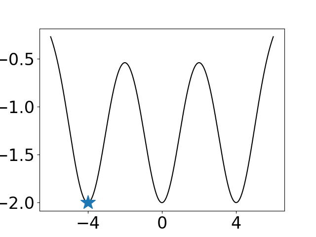
(a) Gaussian

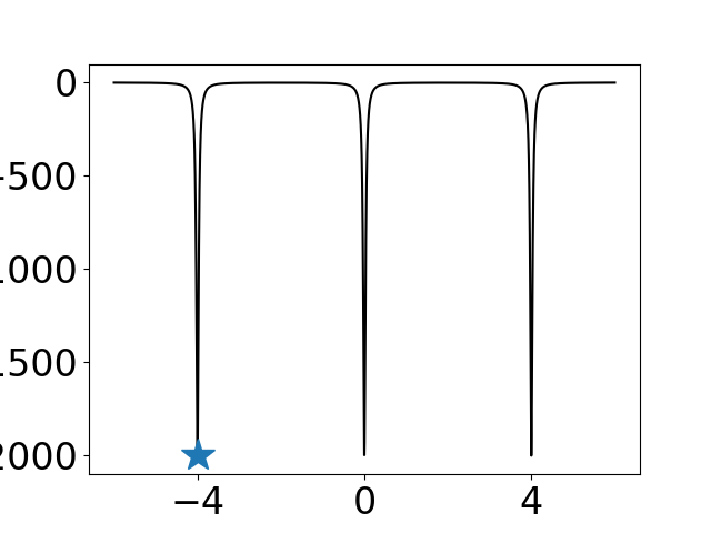
(b) IMQ

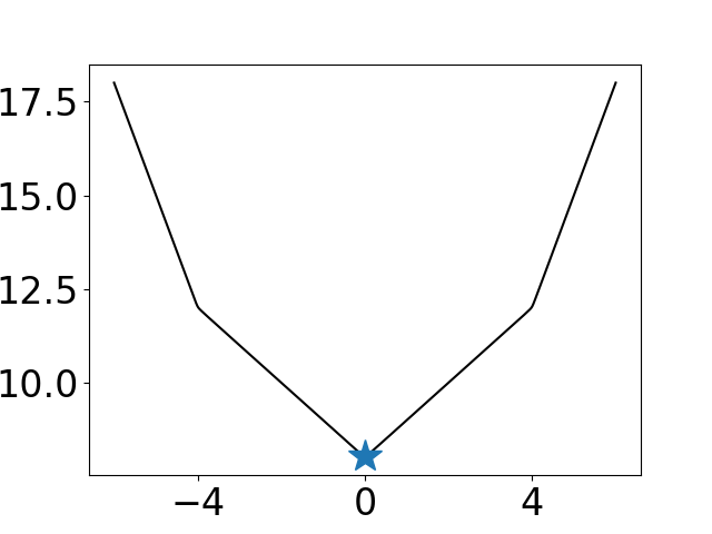
(c) Coulomb

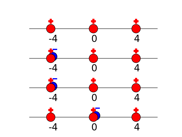
(d) Solution

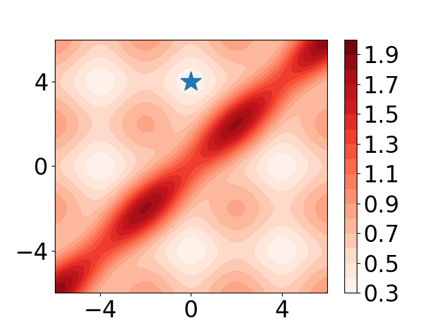
(e) Gaussian

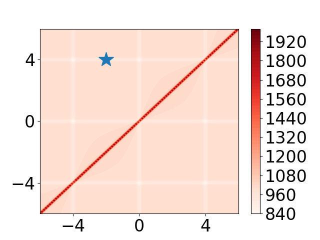
(f) IMQ

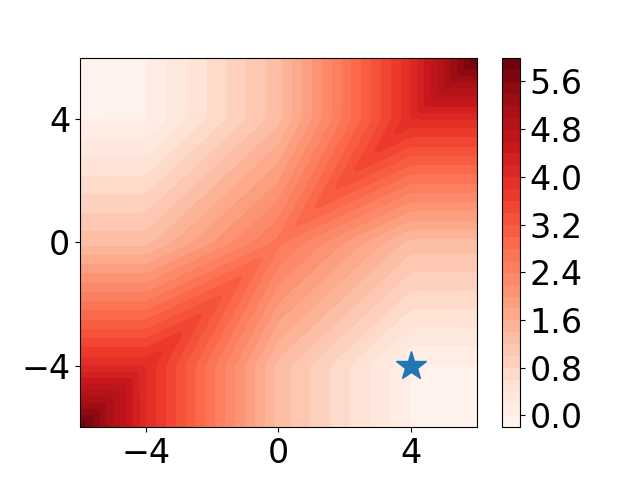
(g) Coulomb

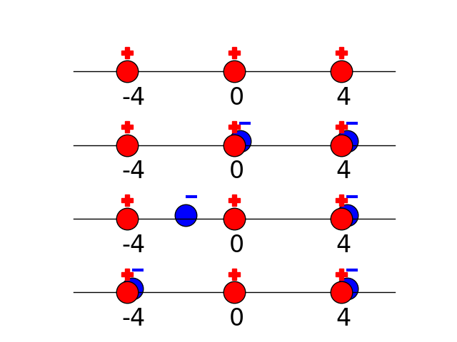
(h) Solution

Figure 1: Monodimensional cases with single ((a)-(d)) and pair of negative charged particles ((e)-(h))). (a-c) and (e-g) are the plots of the regularizer in (1) over different locations of the negative particles for the Gaussian, the inverse quadratic and the Coulomb kernels, respectively. (d) and (h) show possible minimizers (for the respective kernels).

2.1 Convergence properties

The integrals in (1) cannot be computed exactly since $p_{\mathbf{X}}(\mathbf{x})$ is unknown and $q_{\mathbf{Z}}(\mathbf{z})$ is not defined explicitly. As a consequence, we use the unbiased estimate of (1) as a surrogate for optimization, namely:

$$\hat{\mathcal{L}}(f,g){=} \sum_{\mathbf{x}_{i}{\in}\mathcal{D}_{\mathbf{x}}}\frac{\|\mathbf{x}_{i}{-}g(f(\mathbf{x}_{i}))\|^{2}}{N}+\lambda\Bigg{\{}\frac{1}{N(N{-}1)}\sum_{\begin{subarray}{c}\mathbf{z}_{i},\mathbf{z}_{j}{\in}\mathcal{D}_{\mathbf{z}}\\ j\neq i\end{subarray}}k_{i,j}$$

$$-\frac{2}{N^{2}}\sum_{\mathbf{z}_{i}{\in}\mathcal{D}_{\mathbf{z}}}\sum_{\begin{subarray}{c}\mathbf{z}_{j}{\in}\mathcal{D}_{\mathbf{z}}^{f}\end{subarray}}k_{i,j}+\frac{1}{N(N{-}1)}\sum_{\begin{subarray}{c}\mathbf{z}_{i},\mathbf{z}_{j}{\in}\mathcal{D}_{\mathbf{z}}^{f}\\ j\neq i\end{subarray}}k_{i,j}\Bigg{\}}$$ (2)

where $k_{i,j}\doteq k(\mathbf{z}_{i},\mathbf{z}_{j})$ and $\mathcal{D}_{\mathbf{x}}{=}\{\mathbf{x}_{i}\}_{i=1}^{N}$, $\mathcal{D}_{\mathbf{z}}{=}\{\mathbf{z}_{i}\}_{i=1}^{N}$ and $\mathcal{D}_{\mathbf{z}}^{f}{=}\{f(\mathbf{x}_{i})\}_{i=1}^{N}$ are three finite set of samples drawn from $p_{\mathbf{X}}(\mathbf{x})$, $p_{\mathbf{Z}}(\mathbf{z})$ and $q_{\mathbf{Z}}(\mathbf{z})$, respectively.

Note that the MMD term, corresponding to the last three addends in (2), is not convex in the set of unknowns $\mathcal{D}_{\mathbf{z}}^{f}$. This means that it is not possible in general to ensure convergence to the global minimum. Nevertheless, we can prove that, for a specific family of kernels, called Coulomb kernels [12, 31], this property can be achieved. In fact,

Theorem 1.

Assume that

1. $N>h$.

2. $\forall\mathbf{z}_{i},\mathbf{z}_{j}\in\mathcal{D}_{\mathbf{z}},$ $\mathbf{z}_{i}\neq\mathbf{z}_{j}$

3. The kernel function satisfies the Poisson’s equation, namely $-\nabla_{\mathbf{z}}^{2}k(\mathbf{z},\mathbf{z}^{\prime})=\lambda\delta(\mathbf{z}-\mathbf{z}^{\prime}),\quad\forall\mathbf{z},\mathbf{z}^{\prime}\in\mathbb{R}^{h}$. And the solution can be written in the following form

   $$k(\mathbf{z},\mathbf{z}^{\prime})=\left\{\begin{array}[]{ll}-\frac{\lambda}{2\pi}\ln\|\mathbf{z}-\mathbf{z}^{\prime}\|&h=2\\ \frac{\lambda}{\beta\mathcal{S}_{h}\|\mathbf{z}-\mathbf{z}^{\prime}\|^{\beta}}&\beta=h-2,h>2\end{array}\right.$$ (3)

   where $\mathcal{S}_{h}$ is the surface area of a $h$-dimensional unit ball.

Then, the MMD term in (2) satisfies the following general properties:

1. all local extrema are global.

2. the set of saddle points have zero Lebesgue measure.

Furthermore, the set of all global minima is finite and consists of all possible permutations of the elements in $\mathcal{D}_{\mathbf{z}}$. In other words, $\mathcal{D}_{\mathbf{z}}^{f}=\mathcal{D}_{\mathbf{z}}$.

Proof.

Define the MMD term as:

$$\hat{\mathcal{G}}(\{\mathbf{x}_{i}\}_{i=1}^{N},\{\mathbf{z}_{i}\}_{i=1}^{N})$$ (4)

$$=\frac{1}{N(N-1)}\sum_{i=1}^{N}\sum_{j\neq i}k(\mathbf{x}_{i},\mathbf{x}_{j})+\frac{1}{N(N-1)}\sum_{i=1}^{N}\sum_{j\neq i}k(\mathbf{z}_{i},\mathbf{z}_{j})$$

$$-\frac{2}{N^{2}}\sum_{i=1}^{N}\sum_{j=1}^{N}k(\mathbf{x}_{i},\mathbf{z}_{j})$$

By the definition of Poisson kernel, we get the Laplacian of $\hat{\mathcal{G}}$ as

$$\nabla_{\mathbf{x}_{i}}^{2}\hat{\mathcal{G}}=-\frac{2}{N(N-1)}\sum_{j\neq i}\delta(\mathbf{x}_{i}-\mathbf{x}_{j})+\frac{2}{N^{2}}\sum_{j=1}^{N}\delta(\mathbf{x}_{i}-\mathbf{z}_{j})$$ (5)

Thus, $\hat{\mathcal{G}}$ is harmonic except on the set $H=\{\mathbf{x}:\mathbf{x}_{i}\neq\mathbf{x}_{j},\mathbf{x}_{i}\neq\mathbf{z}_{j},\forall i,j=1,...,N\}$. By the Maximal Principle of harmonic functions, $\hat{\mathcal{G}}$ has no local extrema and all the extrema are global.
On the other hand, the saddle points of $\hat{\mathcal{G}}$ satisfy

$$\nabla_{\mathbf{x}_{i}}\hat{\mathcal{G}}= -\frac{1}{N(N-1)}\sum_{j\neq i}\frac{\mathbf{x}_{i}-\mathbf{x}_{j}}{\|\mathbf{x}_{i}-\mathbf{x}_{j}\|^{h}}+$$

$$\frac{1}{N^{2}}\sum_{j=1}^{N}\frac{\mathbf{x}_{i}-\mathbf{z}_{j}}{\|\mathbf{x}_{i}-\mathbf{z}_{j}\|^{h}}=0$$ (6)

This implies that

$$F(\mathbf{x_{i}})\triangleq\sum_{j=1}^{N}\frac{\mathbf{x}_{i}-\mathbf{z}_{j}}{\|\mathbf{x}_{i}-\mathbf{z}_{j}\|^{h}}=\frac{N}{N-1}\sum_{j\neq i}\frac{\mathbf{x}_{i}-\mathbf{x}_{j}}{\|\mathbf{x}_{i}-\mathbf{x}_{j}\|^{h}}$$ (7)

As $\hat{\mathcal{G}}$ is harmonic except on the set $H$, $F$ is analytic except on $H$. By the symmetry of the right hand side, we have $\sum_{i=1}^{N}F(\mathbf{x}_{i})=0$. Define

$$A=\{(\mathbf{x}_{1},...,\mathbf{x}_{N}):\mathbf{x}_{i}\in\mathbb{R}^{h}\backslash\{\mathbf{z}_{i}\}_{i=1}^{N},\sum_{i=1}^{N}F(\mathbf{x}_{i})=0\}$$

If $(\mathbf{x}_{1},...,\mathbf{x}_{N})\in A$, then $\mathbf{x}_{N}\in F^{-1}(-\sum_{i=1}^{N-1}F(\mathbf{x}_{i}))$. By considering that $F$ is analytic and nonconstant and by using the Fubini Theorem we get that the measure of $A$ is

$$|A| =\int_{(\mathbb{R}^{h})^{N}}\chi_{A}d\mathbf{x}_{1}...d\mathbf{x}_{N}$$

$$=\int_{(\mathbb{R}^{h})^{N-1}}(\int_{\mathbb{R}^{h}}\chi_{A}d\mathbf{x}_{N})d\mathbf{x}_{1}...d\mathbf{x}_{N-1}$$

$$=\int_{(\mathbb{R}^{h})^{N-1}}|F^{-1}(-\sum_{i=1}^{N-1}F(\mathbf{x}_{i}))|d\mathbf{x}_{1}...d\mathbf{x}_{N-1}=0$$ (8)

where $\chi_{A}$ is the characteristic function, equals 1 on $A$, otherwise equals 0 and $|\cdot|$ denotes the Lebesgue measure operator. The third equality in (8) holds because we know that for a nonconstant analytic function, its inverse image at a value is of zero measure (w.r.t h-dimensional Lebesgue measure). As the saddle point is a subset of $A$, so the set of saddle points have zero Lebesgue measure. ∎

The assumptions of the theorem are quite general in practice. In fact, the requirement $N>h$ is generally valid in applications involving autoencoders. The second assumption is valid with probability 1, as long as the elements in $\mathcal{D}_{\mathbf{z}}$ are drawn independently from $p_{Z}$.

Note that, since the set of saddle points has zero measure, optimization through local search methods can converge to global minima. This is an important characteristic which is similar to convex functionals. Another important remark is that at optimality, the sets $\mathcal{D}_{\mathbf{z}}^{f}$ and $\mathcal{D}_{\mathbf{z}}$ are equal, independently of the sampling from $p_{Z}$ and of the choice of $N$. Therefore, MMD with Coulomb kernel forces $q_{Z}$ to be equal to $p_{Z}$.

It is important to mention that Coulomb kernels represent a generalization of Coulomb’s law to any $h$-dimensional Euclidean space. Therefore, samples from $p_{\mathbf{Z}}$ and $q_{\mathbf{Z}}$ can be regarded as positive and negative charged particles, respectively, while the Coulomb kernels induce some global attraction and repulsion forces between them. As a consequence, the minimization of the regularizer in (2), with respect to the location of the negative charged particles, allows to find a configuration where the two sets of particles balance each other. Based on this interpretation, we can highlight the differences between Coulomb and other kernels from previous work [30] using two simple mono-dimensional cases ($h=1$). The first example consists of three positive particles, located at $-4,0$ and $4$, and a single negative particle, that is allowed to move freely. In this case, $p_{Z}(z)=\delta(z+4)+\delta(z)+\delta(z-4)$ and $q_{Z}(z)=\delta(z-z_{1})$, where $z_{1}$ represents the variable location of the negative particle. Figure 1(a) and Figure 1(b) represent the plots of the regularizer in (1) evaluated at different $z_{1}$ for the Gaussian, the inverse multiquadratic and the Coulomb kernels, respectively. The Gaussian and the inverse multiquadratic kernels introduce new local optima and the negative particle is attracted locally to one of the positive charges without being affected by the remaining ones. On the contrary, the Coulomb kernel has only a single minimum. This minimal configuration is the best one, if one considers that all positive particles exert an attraction force on the negative one. As a result the Coulomb kernel induces global attraction forces. The second example consists of the same three positive particles and a pair of free negative charges. In this case, $q_{Z}(z)=\delta(z-z_{1})+\delta(z-z_{2})$, where $z_{1},z_{2}$ are the locations of the two negative particles. Figure 1(d) and Figure 1(e) represent the plots of the regularizer in (1) evaluated at different $z_{1},z_{2}$ for the Gaussian, the inverse multiquadratic and the Coulomb kernels, respectively. Following the same reasoning of the previous example, we conclude that the Coulomb kernel induces global repulsion forces.

It is worth mentioning that these theoretical results are valid when the optimization is performed on the function space, namely when minimizing with respect to $f$ and $g$. In reality, the training is performed on the parameter space of neural networks, which may introduce local optima due to their non-convex nature. Solving the problem of local minima in the parameter space of neural networks is a very general problem common to deep learning approaches, which is out of the scope of this work. Our aim is to provide a principled objective function with better convergence properties with respect to existing works.

2.2 Generalization bound

The following theorem provides a probabilistic bound on the estimation error between $\hat{\mathcal{L}}(f,g)$ and $\mathcal{L}(f,g)$ in (2).

Theorem 2.

Given the objective in (2), $h>2$, $\Omega_{\mathbf{z}}$ a compact set, $\Omega_{\mathbf{x}}=[-M,M]^{d}$ for positive scalar $M$, and a symmetric, continuous and positive definite kernel $k:\Omega_{\mathbf{z}}\times\Omega_{\mathbf{z}}\rightarrow\mathbb{R}$, where $0\leq k(\mathbf{z},\mathbf{z}^{\prime})\leq K$ for all $\mathbf{z},\mathbf{z}^{\prime}\in\Omega_{\mathbf{z}}$ with $K=k(\mathbf{z},\mathbf{z})$. If the reconstruction error $\|\mathbf{x}{-}g(f(\mathbf{x}))\|^{2}$ can be made small $\forall\mathbf{x}\in\Omega_{\mathbf{x}}$, such that it can be bounded by a small value $\xi$.

Then, for any $s,u,v,t>0$

$$\text{Pr}\bigg{\{}|\hat{\mathcal{L}}-\mathcal{L}|{>}t+\lambda(s+u+v)\bigg{\}}\leq 2\exp\bigg{\{}{-}\frac{2Nt^{2}}{\xi^{2}}\bigg{\}}$$

$$\quad+2\exp\bigg{\{}{-}\frac{2\lfloor N/2\rfloor s^{2}}{K^{2}}\bigg{\}}+2\exp\bigg{\{}{-}\frac{2\lfloor N/2\rfloor u^{2}}{K^{2}}\bigg{\}}$$

$$\quad+2\exp\bigg{\{}{-}\frac{2Nv^{2}}{K^{2}}\bigg{\}}$$

Proof.

In order to prove the theorem, we first derive the statistical bounds for the reconstruction and the MMD terms separately, and then combine them to obtain the final bound.

Consider the reconstruction error term and define $\xi_{\mathbf{x}}\doteq\|\mathbf{x}{-}g(f(\mathbf{x}))\|^{2}$. Note that $\Omega_{\mathbf{x}}=[-M,M]^{d}$ and therefore $\xi_{\mathbf{x}}$ is bounded in the interval $[0,4M^{2}d]$. By considering $\xi_{\mathbf{x}}$ a random variable, we can apply the Hoeffding’s inequality (see Theorem 2 in [33]) to obtain the following statistical bound:

$$\text{P}_{0}\doteq \text{Pr}\bigg{\{}\bigg{|}\frac{1}{N}{\sum_{\mathbf{x}{\in}\mathcal{D}_{\mathbf{x}}}}\xi_{\mathbf{x}}{-}{\int_{\Omega_{\mathbf{x}}}}\xi_{\mathbf{x}}p_{\mathbf{X}}(\mathbf{x})d\mathbf{x}\bigg{|}\geq 2\exp\bigg{\{}{-}\frac{2Nt^{2}}{\xi^{2}}\bigg{\}}$$ (9)

where $t$ is an arbitrary small positive constant.

We can then proceed to find the bound for the other terms in (2). In particular, using the one-sample and two sample U statistics in [33] (see pag. 25), we obtain the following bounds:

$$\text{P}_{1}\doteq \text{Pr}\bigg{\{}\bigg{|}\frac{1}{N(N{-}1)}\sum_{\begin{subarray}{c}\mathbf{z}_{i},\mathbf{z}_{j}{\in}\mathcal{D}_{\mathbf{z}}\\ j\neq i\end{subarray}}k_{i,j}{-}D(p_{\mathbf{Z}},p_{\mathbf{Z}})\bigg{|}$$

$$\geq s\bigg{\}}\leq 2\exp\bigg{\{}\frac{{-}2\lfloor N/2\rfloor s^{2}}{K^{2}}\bigg{\}}$$

$$\text{P}_{2}\doteq \text{Pr}\bigg{\{}\bigg{|}\frac{1}{N(N{-}1)}\sum_{\begin{subarray}{c}\mathbf{z}_{i},\mathbf{z}_{j}{\in}\mathcal{D}_{\mathbf{z}}^{f}\\ j\neq i\end{subarray}}k_{i,j}{-}D(q_{\mathbf{Z}},q_{\mathbf{Z}})\bigg{|}$$

$$\geq u\bigg{\}}\leq 2\exp\bigg{\{}\frac{{-}2\lfloor N/2\rfloor u^{2}}{K^{2}}\bigg{\}}$$

$$\text{P}_{3}\doteq \text{Pr}\bigg{\{}\bigg{|}-\frac{2}{N^{2}}\sum_{\mathbf{z}_{i}{\in}\mathcal{D}_{\mathbf{z}}}\sum_{\mathbf{z}_{j}{\in}\mathcal{D}_{\mathbf{z}}^{f}}k_{i,j}+2D(p_{\mathbf{Z}},q_{\mathbf{Z}})\bigg{|}$$

$$\geq v\bigg{\}}\leq 2\exp\bigg{\{}\frac{{-}2Nv^{2}}{K^{2}}\bigg{\}}$$ (10)

where $D(p_{\mathbf{Z}},q_{\mathbf{Z}})\doteq\int_{\Omega_{\mathbf{z}}}\int_{\Omega_{\mathbf{z}}}p_{\mathbf{Z}}(\mathbf{z})q_{\mathbf{Z}}(\mathbf{z}^{\prime})k(\mathbf{z},\mathbf{z}^{\prime})d\mathbf{z}d\mathbf{z}^{\prime}$. Then, we can get the following lower bound:

$$\sum_{i=0}^{3}\text{P}_{i} \geq\text{Pr}\bigg{\{}\bigg{|}\frac{1}{N}{\sum_{\mathbf{x}{\in}\mathcal{D}_{\mathbf{x}}}}\xi_{\mathbf{x}}{-}{\int_{\Omega_{\mathbf{x}}}}\xi_{\mathbf{x}}p_{\mathbf{X}}(\mathbf{x})d\mathbf{x}\bigg{|}\geq t\quad\cup$$

$$\quad\quad\bigg{|}\frac{1}{N(N{-}1)}\sum_{\begin{subarray}{c}\mathbf{z}_{i},\mathbf{z}_{j}{\in}\mathcal{D}_{\mathbf{z}}\\ j\neq i\end{subarray}}k_{i,j}-D(p_{\mathbf{Z}},p_{\mathbf{Z}})\bigg{|}\geq s\quad\cup$$

$$\quad\quad\bigg{|}\frac{1}{N(N{-}1)}\sum_{\begin{subarray}{c}\mathbf{z}_{i},\mathbf{z}_{j}{\in}\mathcal{D}_{\mathbf{z}}^{f}\\ j\neq i\end{subarray}}k_{i,j}-D(q_{\mathbf{Z}},q_{\mathbf{Z}})\bigg{|}\geq u\quad\cup$$

$$\quad\quad\bigg{|}-\frac{2}{N^{2}}\sum_{\mathbf{z}_{i}{\in}\mathcal{D}_{\mathbf{z}}}\sum_{\mathbf{z}_{j}{\in}\mathcal{D}_{\mathbf{z}}^{f}}k_{i,j}+2D(p_{\mathbf{Z}},q_{\mathbf{Z}})\bigg{|}\geq v\bigg{\}}$$

$$=\text{Pr}\bigg{\{}\bigg{|}\frac{1}{N}{\sum_{\mathbf{x}{\in}\mathcal{D}_{\mathbf{x}}}}\xi_{\mathbf{x}}{-}{\int_{\Omega_{\mathbf{x}}}}\xi_{\mathbf{x}}p_{\mathbf{X}}(\mathbf{x})d\mathbf{x}\bigg{|}\geq t\quad\cup$$

$$\quad\quad\lambda\bigg{|}\frac{1}{N(N{-}1)}\sum_{\begin{subarray}{c}\mathbf{z}_{i},\mathbf{z}_{j}{\in}\mathcal{D}_{\mathbf{z}}\\ j\neq i\end{subarray}}k_{i,j}-D(p_{\mathbf{Z}},p_{\mathbf{Z}})\bigg{|}\geq\lambda s\quad\cup$$

$$\quad\quad\lambda\bigg{|}\frac{1}{N(N{-}1)}\sum_{\begin{subarray}{c}\mathbf{z}_{i},\mathbf{z}_{j}{\in}\mathcal{D}_{\mathbf{z}}^{f}\\ j\neq i\end{subarray}}k_{i,j}-D(q_{\mathbf{Z}},q_{\mathbf{Z}})\bigg{|}\geq\lambda u\quad\cup$$

$$\quad\quad\lambda\bigg{|}-\frac{2}{N^{2}}\sum_{\mathbf{z}_{i}{\in}\mathcal{D}_{\mathbf{z}}}\sum_{\mathbf{z}_{j}{\in}\mathcal{D}_{\mathbf{z}}^{f}}k_{i,j}+2D(p_{\mathbf{Z}},q_{\mathbf{Z}})\bigg{|}\geq\lambda v\bigg{\}}$$

$$\geq\text{Pr}\bigg{\{}\bigg{|}\frac{1}{N}{\sum_{\mathbf{x}{\in}\mathcal{D}_{\mathbf{x}}}}\xi_{\mathbf{x}}{-}{\int_{\Omega_{\mathbf{x}}}}\xi_{\mathbf{x}}p_{\mathbf{X}}(\mathbf{x})d\mathbf{x}+\lambda\frac{1}{N(N{-}1)}\sum_{\begin{subarray}{c}\mathbf{z}_{i},\mathbf{z}_{j}{\in}\mathcal{D}_{\mathbf{z}}\\ j\neq i\end{subarray}}k_{i,j}$$

$$\quad\quad-\lambda D(p_{\mathbf{Z}},p_{\mathbf{Z}})+\frac{1}{N(N{-}1)}\lambda\sum_{\begin{subarray}{c}\mathbf{z}_{i},\mathbf{z}_{j}{\in}\mathcal{D}_{\mathbf{z}}^{f}\\ j\neq i\end{subarray}}k_{i,j}$$

$$\quad\quad-\lambda D(q_{\mathbf{Z}},q_{\mathbf{Z}})-\frac{2}{N^{2}}\lambda\sum_{\mathbf{z}_{i}{\in}\mathcal{D}_{\mathbf{z}}}\sum_{\mathbf{z}_{j}{\in}\mathcal{D}_{\mathbf{z}}^{f}}k_{i,j}$$

$$\quad\quad+2\lambda D(p_{\mathbf{Z}},q_{\mathbf{Z}})\bigg{|}\geq t+\lambda(s+u+v)\bigg{\}}$$

$$\geq\text{Pr}\bigg{\{}\bigg{|}\frac{1}{N}{\sum_{\mathbf{x}{\in}\mathcal{D}_{\mathbf{x}}}}\xi_{\mathbf{x}}+\lambda\bigg{[}\frac{1}{N(N{-}1)}\sum_{\begin{subarray}{c}\mathbf{z}_{i},\mathbf{z}_{j}{\in}\mathcal{D}_{\mathbf{z}}\\ j\neq i\end{subarray}}k_{i,j}$$

$$\quad\quad\frac{1}{N(N{-}1)}\sum_{\begin{subarray}{c}\mathbf{z}_{i},\mathbf{z}_{j}{\in}\mathcal{D}_{\mathbf{z}}^{f}\\ j\neq i\end{subarray}}k_{i,j}-\frac{2}{N^{2}}\sum_{\mathbf{z}_{i}{\in}\mathcal{D}_{\mathbf{z}}}\sum_{\mathbf{z}_{j}{\in}\mathcal{D}_{\mathbf{z}}^{f}}k_{i,j}\bigg{]}$$

$$\quad\quad{-}{\int_{\Omega_{\mathbf{x}}}}\xi_{\mathbf{x}}p_{\mathbf{X}}(\mathbf{x})d\mathbf{x}-\lambda\bigg{[}D(p_{\mathbf{Z}},p_{\mathbf{Z}})+D(q_{\mathbf{Z}},q_{\mathbf{Z}})+$$

$$\quad\quad-2D(p_{\mathbf{Z}},q_{\mathbf{Z}})\bigg{]}\bigg{|}\geq t+\lambda(s+u+v)\bigg{\}}$$

$$=\text{Pr}\bigg{\{}\bigg{|}\hat{\mathcal{L}}{-}{\int_{\Omega_{\mathbf{x}}}}\xi_{\mathbf{x}}p_{\mathbf{X}}(\mathbf{x})d\mathbf{x}$$

$$\quad\quad-\lambda\bigg{[}\int_{\Omega_{\mathbf{z}}}\int_{\Omega_{\mathbf{z}}}(p_{\mathbf{Z}}(\mathbf{z})-q_{\mathbf{Z}}(\mathbf{z}))(p_{\mathbf{Z}}(\mathbf{z}^{\prime})$$

$$\quad\quad-q_{\mathbf{Z}}(\mathbf{z}^{\prime}))k(\mathbf{z},\mathbf{z}^{\prime})d\mathbf{z}d\mathbf{z}^{\prime}\bigg{]}\bigg{|}\geq t+\lambda(s+u+v)\bigg{\}}$$

$$=\text{Pr}\bigg{\{}\bigg{|}\hat{\mathcal{L}}{-}\mathcal{L}\bigg{|}\geq t+\lambda(s+u+v)\bigg{\}}$$

where the first inequality is obtained by applying the union bound. Finally, by exploiting also the results in (9), (10) we get the desired bound. ∎

Theorem 2 provides a probabilistic bound on the estimation error between $\hat{\mathcal{L}}(f,g)$ and $\mathcal{L}(f,g)$. The bound consists of four terms which vanish when $N$ is large. It is important to mention that, while the last three terms can be made arbitrarily small, by choosing appropriate values for $s,u,v$ and $\lambda$, the first term depends mainly on on the value of $\xi$, which can be controlled by modifying the capacity of the encoding and the decoding networks. Therefore, we can improve the generalization performance of the model by controlling the capacity of the networks as long as $\xi$ can be made small. This is confirmed also in practice, as shown in the experimental section.

3 Related Work

The most promising research directions for implicit generative models are generative adversarial networks (GANs) and autoencoder-based models.

GANs [9] cast the problem of density estimation as a mini-max game between two neural networks, namely a discriminator, that tries to distinguish between true and generated samples, and a generator, that tries to produce samples similar to the true ones, to fool the discriminator. GANs are notoriously difficult to train, usually requiring careful design strategies for network architectures in [4]. Some of the most known issues are (i) the problem of vanishing gradients in [21], which happens when the output of the discriminator is saturated, because true and generated data are perfectly classified, and no more gradient information is provided to the generator, (ii) the problem of mode collapse in [16], which happens when the samples from the generator collapse to a single point corresponding to the maximum output value of the discriminator, and (iii) the problem of instability associated with the failure of convergence, which is due to the intrinsic nature of the mini-max problem. Different line of works [9] [27] [13] [23] [16] [29], have proposed effective solutions to overcome the aforementioned issues with GANs. However, all these strategies have either poor theoretical motivation or they are guaranteed to converge only locally.

Another research direction for GANs consists on using integral probability metrics [2] as optimization objective. In particular, the maximum mean discrepancy [10] can be used to measure the distance between $p_{\mathbf{X}}$ and $q_{\mathbf{Y}}$ and train the generator network. The general problem is formulated in the following way:

$$\inf_{g\in\mathcal{G}}\sup_{f\in\mathcal{F}}\big{\{}E_{\mathbf{x}\sim p_{\mathbf{X}}}[f(\mathbf{x})]-E_{\mathbf{y}\sim q_{\mathbf{Y}}}[f(\mathbf{y})]\big{\}}\\$$

In generative moment matching networks [19, 8] $\mathcal{F}$ is a RKHS, which is induced by the Gaussian kernel. Note that a major limitation of these models is the curse of dimensionality, since the similarity scores associated with the kernel function are directly computed in the sample space, as explained in [25]. The work of [17] introduces an encoding function to represent data in a more compact way and distances are computed in the latent representation, thus solving the problem of dimensionality. [24] propose to extend the maximum mean discrepancy and include also covariance statistics to ensure better stability. The work of [30] generalizes the computation of the distance between the encoded distribution and the prior to other divergences, thus proposing two different solutions: the first one consists of using the Jensen-Shannon divergence, showing also the equivalence to adversarial autoencoders, and the second one consists of using the maximum-mean discrepancy. The choice of the kernel function in this second case is of fundamental importance to ensure the global convergence of gradient-descent algorithms. As we have already shown in previous section, suboptimal choices of the kernel function, like the ones used by the authors, introduce local optima in the function space and therefore do not have the same convergence property of our model. The work by [31] use Coulomb kernels under the GANs’ framework. Nevertheless, the computation of distances is performed directly in the sample space, thus being negatively affected by the curse of dimensionality.

There exists other autoencoder-based models that are inspired by the adversarial game of GANs. [5] add an autoencoder network to the original GANs for reconstructing part of the latent code. The identical works of [14] and [32] propose to add an encoding function together with the generator and perform an adversarial game to ensure that the joint density on the input/output of the generator agrees with the joint density of the input/output of the encoder. They prove that the optimal solution is achieved when the generator and the encoder are invertible. In practice, they fail to guarantee the convergence to that solution due to the adversarial nature of the game. [28] extend the previous works by explicitly imposing the invertibility condition. They achieve this by adding a term to the generator objective that computes the reconstruction error on the latent space. Adversarial autoencoders by [1] are similar to these approaches with the only differences that the estimation of the reconstruction error is performed in the sample space, while the adversarial game is performed only in the latent space. It is important to mention that all of these works are based on a mini-max problem, while our method solves a simple minimization problem, which behaves better in terms of training convergence.

Variational autoencoders (VAEs) by [6, 26] represent another family of autoencoder-based models. The framework is based on minimizing the Kullback-Leibler (KL) divergence between the approximate posterior distribution defined by the encoder and the true prior $p_{\mathbf{Z}}$ (which consists of a surrogate for the negative log-likelihood of training data). Practically speaking, the stochastic encoder used in variational autoencoders is driven to produce latent representations that can be similar among different input samples, thus generating conflicts during reconstruction. A deterministic encoder could ideally solve this problem, but unfortunately the KL divergence is not defined for such case. There are several variations for VAEs. For example, the work in [22] proposes to use the adversarial game of GANs to learn better approximate posterior distributions in VAEs. Nevertheless, the method is still based on a mini-max problem. Recently, [7] propose a training strategy based on a cascade of two VAEs to deal with the limitations implied by the KL divergence. In particular, the authors train a first VAE on the training data and then train a second VAE on the learnt latent representations. This second step is fundamental to improve the matching between the posterior density and the prior with respect to what is done in the first stage. Therefore, this solution implicitly considers the mitigation of local minima from the level of architecture design. However, the 2-stage procedure does not prevent local minima induced by the combination of the two addends in the two objectives. To the best of our knowledge, only [20] are aware of the problem of local minima in generative autoencoders. The authors analyze theoretically the behaviour of simple linear VAEs and show that the phenomenon known as posterior collapse is due to the problem of local minima (or equivalently local maxima, when considering to maximize the ELBO).

4 Experiments

We evaluate the performance of our model (CouAE) against the baseline of Variational Autoencoders (VAE) [6, 26] and Wasserstein Autoencoders (WAE) [30]. All experiments are performed on two synthetic datasets, to simulate scenarios with low and high dimensional feature spaces and on a real-world faces’ dataset, namely CelebA 64x64.

We distinguish between two sets of experiments. The first set confirms the usefulness of using the MMD coupled with the Coulomb kernel, while the second one aims at validating the generalization error bound in Theorem 2.

4.1 Comparison with other autoencoders

Table 1: Comparison among different autoencoders on different datasets.

Eval. Metric	Data/Method	VAE	WAE	CouAE
Test Log-likel.	Grid	-4.4$\pm$0.2	-6.4$\pm$1.1	-4.3$\pm$0.1
FID	CelebA	63	55	47

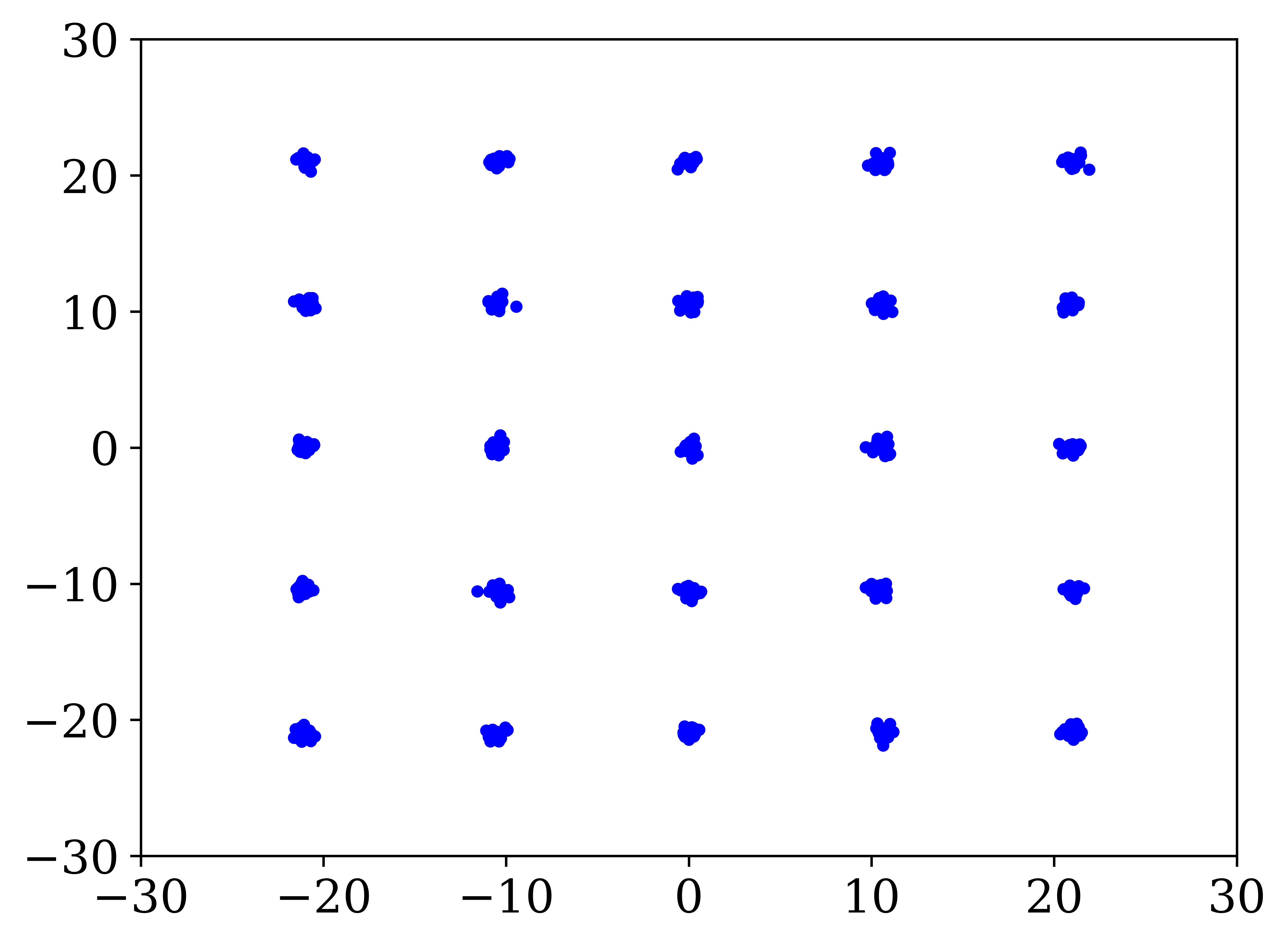
(a) True Data

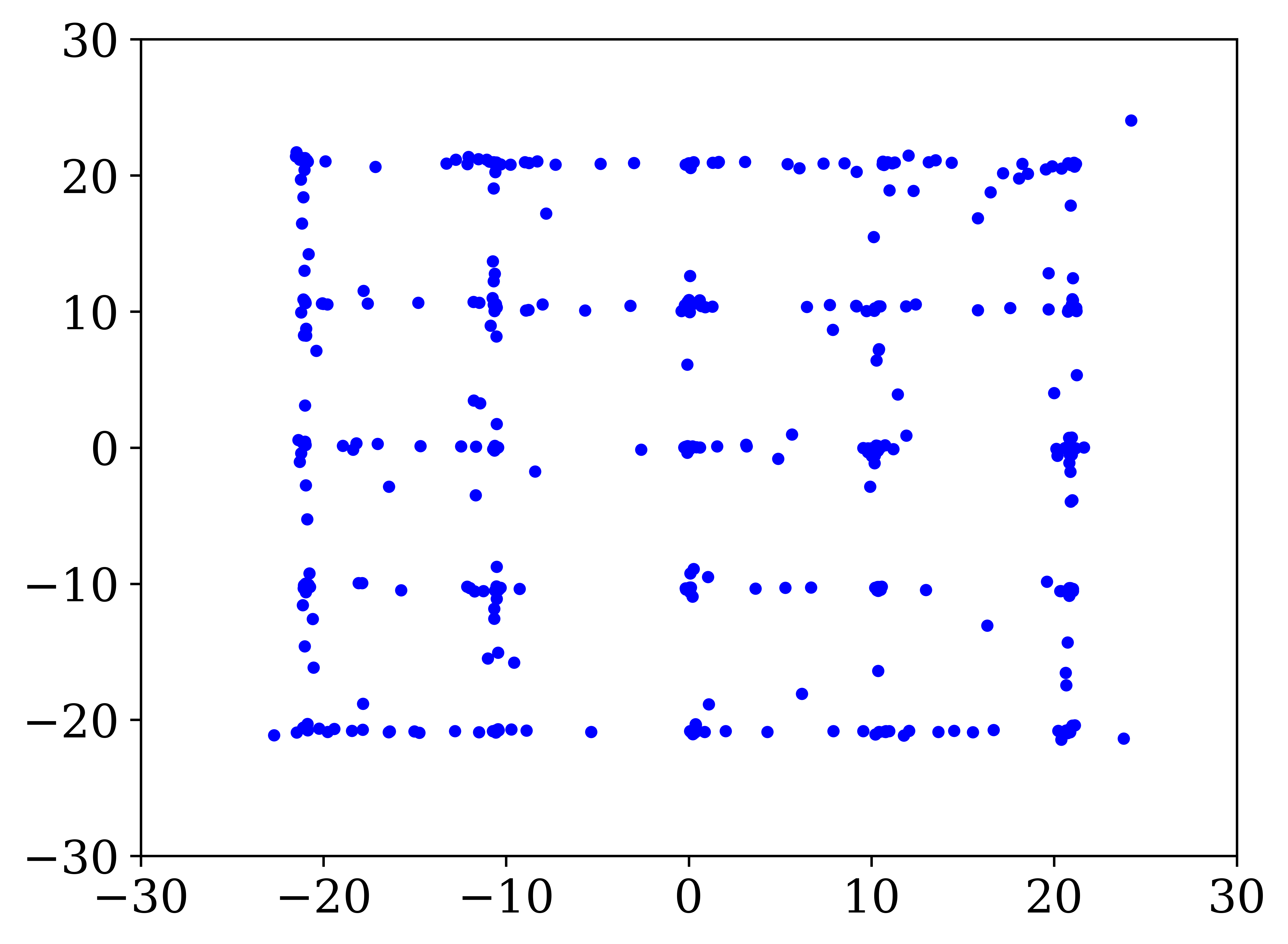
(b) VAE

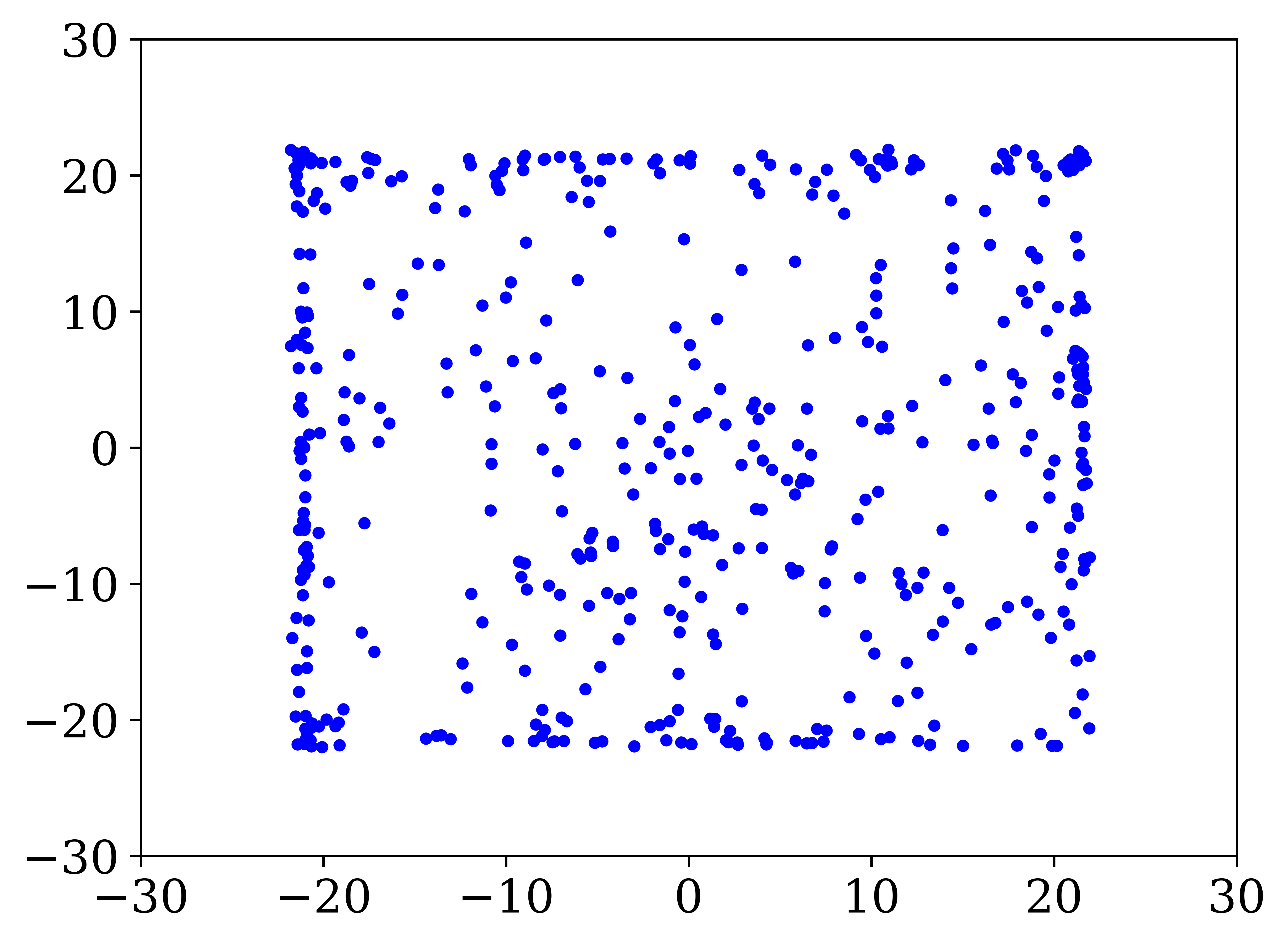
(c) WAE

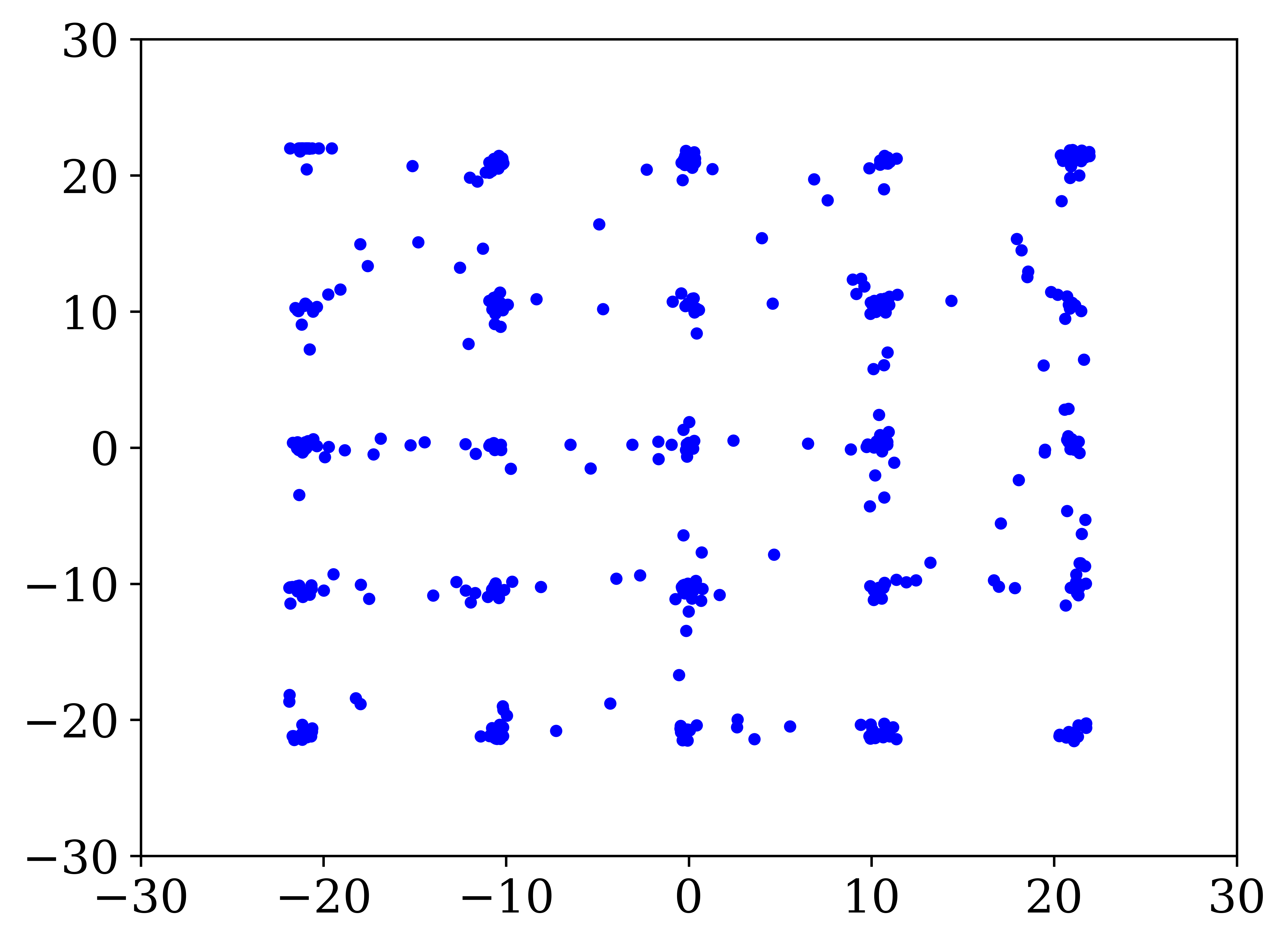
(d) CouAE

Figure 2: Generated data from different models on grid dataset.

(a) VAE

(b) WAE

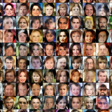
(c) CouAE

Figure 3: Generated samples on CelebA.

We start by comparing the approaches on a two-dimensional dataset consisting of 25 isotropic Gaussians placed according to a grid (see Figure 2(a)), hereafter called the grid dataset [15]. The training dataset contains $500$ samples generated from the true density.

Following the methodology of other works (see for example [15, 31], we choose fully connected Multilayer Perceptrons with two hidden layers (128 neurons each) at both the encoder and the decoder and set $h=2$. All models are trained for $3.10^{6}$ iterations using Adam optimizer with learning rate $10^{-3}$. Models are evaluated qualitatively by visually inspecting generated samples and quantitatively by computing the log-likelihood on test data. To compute the log-likelihood, we first apply kernel density estimation using a Gaussian kernel on $10^{4}$ generated samples and then evaluate the log-likelihood on $10^{4}$ test samples from the true distribution. Results are averaged over $10$ repetitions.

Figure 2 shows samples generated by all models, while Table 1 provides quantitative results in terms of test log-likelihood. These experiments highlight the fact that an improper choice of the kernel function may lead to worse performance. In fact, note that WAE does not perform as good as our proposed solution.

For the experiments on CelebA, we follow the settings used in [30]. In particular, we choose a DCGAN architecture [4] and train all models for $10^{5}$ iterations with a learning rate of $0.0005$. For the competitors, we run the simulations using the implementation of [4]. Figure 3 shows samples generated by all models, while Table 1 provides quantitative results in terms of test FID [11]. These experiments confirm the findings observed on the grid and the low-dimensional embedding datasets, namely that the choice of using the MMD coupled with the Coulomb kernel provides significant improvements over VAEs and WAEs.

4.2 Validation of generalization bound

Table 2: Experimental validation of generalization bound for CouAE. A scaling factor is applied to the number of neurons in each hidden layer to control the capacity of the encoder and the decoder.

Eval. Metric	Data/Width factor	$\times 0.25$	$\times 0.5$	$\times 1$
Test Log-likel.	Grid	-5.8$\pm$0.4	-4.8$\pm$0.4	-4.3$\pm$0.1
Eval. Metric	Data/Width factor	$\times 0.25$	$\times 0.5$	$\times 1$
FID	CelebA	53	51	47

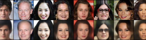
(a) $\times 0.25$

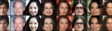
(b) $\times 0.5$

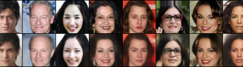
(c) $\times 1$

Figure 4: Reconstruction of test images for different width factors. The top and the bottom row of each case contains the original and reconstructed test images.

To validate the properties of the generalization bound in Theorem 2, we perform experiments on the same datasets used in the previous set of experiments and analyze the performance of CouAE as the capacity of the encoder and the decoder networks changes. In particular, we use the total number of hidden neurons as a proxy to measure the capacity of the model and vary this number according to different scaling factors. Table 2 provides a quantitative analysis of the generalization performance of CouAE. In all cases, we see that an increase of capacity translates into an improvement of the performance. Nevertheless, it is important to mention that there is a limit on the growth of the networks’ capacity. As suggested by Theorem 2, the growth is mainly limited by $\xi$, which could be estimated averaging the reconstruction error on the train and the validation data. In fact, there is no additional benefit to consider larger networks, once $\xi$ is at its minimum, as the bound in Theorem 2 is dominated by the MMD term, which can be improved only by increasing the number of samples. Figure 4 provides a more qualitative analysis on the relation between generalization and reconstruction error. In particular, we visualize some reconstructed test images from the model and see that an increase of the network capacity allows to capture more details about the original images.

It is important to mention that there are also other architectural factors, which may affect the estimation of $\xi$, and which is worth considering in future research. Some examples are the depth of the networks and the use of residual connections (to mitigate the problem of local minima [18]).

5 Conclusions

In this work, we have proposed new theoretical insights on MMD-based autoencoders. In particular, (i) we have proved that MMD coupled with Coulomb kernels has convergence properties similar to convex functionals and shown that these properties have also an impact on the performance of autoencoders, and (ii) we have provided a probabilistic bound on the generalization performance and given principled insights on it.

Appendix A Properties of regularizer in (1)

Lemma 1.

Given $k:\Omega_{\mathbf{z}}\times\Omega_{\mathbf{z}}\rightarrow\mathbb{R}$ a symmetric positive definite kernel, then:

• [3] there exists a unique Hilbert space $\mathcal{H}$ of real-valued functions over $\Omega_{\mathbf{z}}$, for which $k$ is a reproducing kernel. $\mathcal{H}$ is therefore a Reproducing kernel Hilbert Space (RKHS).

• For all $\ell\in\mathcal{H}$

  $$\int_{\Omega_{\mathbf{z}}}\int_{\Omega_{\mathbf{z}}}\phi_{t}(\mathbf{z})\phi_{t}(\mathbf{z}^{\prime})k(\mathbf{z}{,}\mathbf{z}^{\prime})d\mathbf{z}d\mathbf{z}^{\prime}=\text{MMD}^{2}(p_{\mathbf{Z}},q_{\mathbf{Z}})$$

  where

  $$\text{MMD}(p_{\mathbf{Z}},q_{\mathbf{Z}})\doteq\sup_{\|\ell\|_{\mathcal{H}}\leq 1}\big{\{}E_{\mathbf{z}\sim p_{\mathbf{Z}}}[\ell(\mathbf{z})]-E_{\mathbf{z}\sim q_{\mathbf{Z}}}[\ell(\mathbf{z})]\big{\}}$$

  is the maximum mean discrepancy between $p_{\mathbf{Z}}(\mathbf{z})$ and $q_{\mathbf{Z}}(\mathbf{z})$.

• [10] Let $\mathcal{H}$ be defined as in (b), then $\text{MMD}(p_{\mathbf{Z}},q_{\mathbf{Z}})=0$ if and only if $p_{\mathbf{Z}}(\mathbf{z})=q_{\mathbf{Z}}(\mathbf{z})$.

Proof.

(a) follows directly from the Moore-Aronszajn theorem [3].

Now we prove statement (b). For the sake of notation compactness, define $J\doteq\int_{\Omega_{\mathbf{z}}}\int_{\Omega_{\mathbf{z}}}\phi_{t}(\mathbf{z})\phi_{t}(\mathbf{z}^{\prime})k(\mathbf{z}{,}\mathbf{z}^{\prime})d\mathbf{z}d\mathbf{z}^{\prime}$. Therefore,

$$J =\int_{\Omega_{\mathbf{z}}}\int_{\Omega_{\mathbf{z}}}p_{\mathbf{Z}}(\mathbf{z})p_{\mathbf{Z}}(\mathbf{z}^{\prime})k(\mathbf{z}{,}\mathbf{z}^{\prime})d\mathbf{z}d\mathbf{z}^{\prime}-$$

$$\quad-\int_{\Omega_{\mathbf{z}}}\int_{\Omega_{\mathbf{z}}}p_{\mathbf{Z}}(\mathbf{z})q(\mathbf{z}^{\prime})k(\mathbf{z}{,}\mathbf{z}^{\prime})d\mathbf{z}d\mathbf{z}^{\prime}-$$

$$\quad-\int_{\Omega_{\mathbf{z}}}\int_{\Omega_{\mathbf{z}}}p_{\mathbf{Z}}(\mathbf{z}^{\prime})q_{\mathbf{Z}}(\mathbf{z})k(\mathbf{z}{,}\mathbf{z}^{\prime})d\mathbf{z}d\mathbf{z}^{\prime}+$$

$$\quad+\int_{\Omega_{\mathbf{z}}}\int_{\Omega_{\mathbf{z}}}q(\mathbf{z}^{\prime})q_{\mathbf{Z}}(\mathbf{z})k(\mathbf{z}{,}\mathbf{z}^{\prime})d\mathbf{z}d\mathbf{z}^{\prime}$$

$$=\int_{\Omega_{\mathbf{z}}}\int_{\Omega_{\mathbf{z}}}p_{\mathbf{Z}}(\mathbf{z})p_{\mathbf{Z}}(\mathbf{z}^{\prime})\langle r(\mathbf{z}),r(\mathbf{z}^{\prime})\rangle_{\mathcal{H}}d\mathbf{z}d\mathbf{z}^{\prime}-$$

$$\quad-\int_{\Omega_{\mathbf{z}}}\int_{\Omega_{\mathbf{z}}}p_{\mathbf{Z}}(\mathbf{z})q(\mathbf{z}^{\prime})\langle r(\mathbf{z}),r(\mathbf{z}^{\prime})\rangle_{\mathcal{H}}d\mathbf{z}d\mathbf{z}^{\prime}-$$

$$\quad-\int_{\Omega_{\mathbf{z}}}\int_{\Omega_{\mathbf{z}}}p_{\mathbf{Z}}(\mathbf{z}^{\prime})q_{\mathbf{Z}}(\mathbf{z})\langle r(\mathbf{z}),r(\mathbf{z}^{\prime})\rangle_{\mathcal{H}}d\mathbf{z}d\mathbf{z}^{\prime}+$$

$$\quad+\int_{\Omega_{\mathbf{z}}}\int_{\Omega_{\mathbf{z}}}q(\mathbf{z}^{\prime})q_{\mathbf{Z}}(\mathbf{z})\langle r(\mathbf{z}),r(\mathbf{z}^{\prime})\rangle_{\mathcal{H}}d\mathbf{z}d\mathbf{z}^{\prime}$$

$$=\langle E_{\mathbf{z}\sim p_{\mathbf{Z}}}[r(\mathbf{z})],E_{\mathbf{z}^{\prime}\sim p_{\mathbf{Z}}}[r(\mathbf{z}^{\prime})])\rangle_{\mathcal{H}}-$$

$$\quad-\langle E_{\mathbf{z}\sim p_{\mathbf{Z}}}[r(\mathbf{z})],E_{\mathbf{z}^{\prime}\sim q}[r(\mathbf{z}^{\prime})])\rangle_{\mathcal{H}}-$$

$$\quad-\langle E_{\mathbf{z}^{\prime}\sim p_{\mathbf{Z}}}[r(\mathbf{z}^{\prime})],E_{\mathbf{z}\sim q}[r(\mathbf{z})])\rangle_{\mathcal{H}}+$$

$$\quad+\langle E_{\mathbf{z}^{\prime}\sim q}[r(\mathbf{z}^{\prime})],E_{\mathbf{z}\sim q}[r(\mathbf{z})])\rangle_{\mathcal{H}}$$ (11)

Note that the second equality in (11) follows from the fact that $k(\mathbf{z}{,}\mathbf{z}^{\prime})=\langle r(\mathbf{z}),r(\mathbf{z}^{\prime})\rangle_{\mathcal{H}}$ for a unique $r\in\mathcal{H}$, where $\langle\cdot{,}\cdot\rangle_{\mathcal{H}}$ is the inner product of $\mathcal{H}$. If we define $\mu_{p_{\mathbf{Z}}}\doteq E_{\mathbf{z}\sim p_{\mathbf{Z}}}[r(\mathbf{z})]$ and $\mu_{q}\doteq E_{\mathbf{z}\sim q}[r(\mathbf{z})]$, then (11) can be rewritten in the following way:

$$J =\langle\mu_{p_{\mathbf{Z}}}{,}\mu_{p_{\mathbf{Z}}}\rangle_{\mathcal{H}}-\langle\mu_{p_{\mathbf{Z}}}{,}\mu_{q}\rangle_{\mathcal{H}}-\langle\mu_{p_{\mathbf{Z}}}{,}\mu_{q}\rangle_{\mathcal{H}}+\langle\mu_{q}{,}\mu_{q}\rangle_{\mathcal{H}}$$

$$=\langle\mu_{p_{\mathbf{Z}}}-\mu_{q}{,}\mu_{p_{\mathbf{Z}}}-\mu_{q}\rangle_{\mathcal{H}}$$

$$=\|\mu_{p_{\mathbf{Z}}}-\mu_{q}\|_{\mathcal{H}}^{2}$$ (12)

Notice that

$$\|\mu_{p_{\mathbf{Z}}}{-}\mu_{q}\|_{\mathcal{H}} =\Big{\langle}\mu_{p_{\mathbf{Z}}}-\mu_{q}{,}\frac{\mu_{p_{\mathbf{Z}}}-\mu_{q}}{\|\mu_{p_{\mathbf{Z}}}-\mu_{q}\|_{\mathcal{H}}}\Big{\rangle}_{\mathcal{H}}$$

$$=\sup_{\|\ell\|_{\mathcal{H}}\leq 1}\Big{\{}\langle\mu_{p_{\mathbf{Z}}}-\mu_{q},\ell\rangle_{\mathcal{H}}\Big{\}}$$

$$=\sup_{\|\ell\|_{\mathcal{H}}\leq 1}\Big{\{}E_{\mathbf{z}\sim p_{\mathbf{Z}}}[\langle r(\mathbf{z}),\ell\rangle_{\mathcal{H}}]-E_{\mathbf{z}\sim q}[\langle r(\mathbf{z}),\ell\rangle_{\mathcal{H}}]\Big{\}}$$

$$=\sup_{\|\ell\|_{\mathcal{H}}\leq 1}\big{\{}E_{\mathbf{z}\sim p_{\mathbf{Z}}}[\ell(\mathbf{z})]-E_{\mathbf{z}\sim q}[\ell(\mathbf{z})]\big{\}}$$

$$=\text{MMD}(p_{\mathbf{Z}},q_{\mathbf{Z}})$$

Substituting this result into (12) concludes the proof of the statement.

Statement (c) is equivalent to Theorem 3 in [10]. ∎

Appendix B Sufficient conditions for global convergence

This section aims at clarifying the theory proposed in [12]. Note that the authors have focused on proving that the Poisson’s equation is necessary for achieving global convergence. Here, we prove that this equation represents a sufficient condition to guarantee the global convergence on the regularizer in (1), thus motivating the use of Coulomb kernels. The result of the following proposition implies that the loss function associated with the second addend in (1) is free from saddle points and all local minima are global.

Proposition 1.

Assume that the encoder network has enough capacity to achieve the global minimum of the second addend in (1). Furthermore, assume that the kernel function satisfies the Poisson’s equation, viz. $\nabla_{\mathbf{z}}^{2}k(\mathbf{z},\mathbf{z}^{\prime})=-\delta(\mathbf{z}-\mathbf{z}^{\prime})$. Then,

$$|\phi_{t}(\mathbf{z}_{max})|=\frac{1}{\sqrt{2t+(\phi_{0}(\mathbf{z}_{max}))^{-2}}}$$ (13)

where $\phi_{t}(\cdot)$ represents $\phi(\cdot)$ at iteration $t$, while $\mathbf{z}_{max}=\text{arg}\max_{\mathbf{z}}\|\phi_{t}(\mathbf{z})\|$. Therefore, gradient descent-based training converges to the global minimum of the second addend in (1) and at the global minimum $\phi(\mathbf{z})=0$ for all $\mathbf{z}\in\Omega_{\mathbf{z}}$.

Proof.

By defining the potential function at location $\mathbf{z}$, namely $\Psi(\mathbf{z})\doteq\int_{\Omega_{\mathbf{z}}}\phi_{t}(\mathbf{z}^{\prime})k(\mathbf{z},\mathbf{z}^{\prime})d\mathbf{z}^{\prime}$, the second addend in (1) can be rewritten in the following way:

$$\int_{\Omega_{\mathbf{z}}}\int_{\Omega_{\mathbf{z}}}\phi(\mathbf{z})\phi(\mathbf{z}^{\prime})k(\mathbf{z},\mathbf{z}^{\prime})d\mathbf{z}d\mathbf{z}^{\prime} =\int_{\Omega_{\mathbf{z}}}\phi_{t}(\mathbf{z})\Psi(\mathbf{z})d\mathbf{z}$$

$$\doteq\int_{\Omega_{\mathbf{z}}}J(\mathbf{z})d\mathbf{z}$$ (14)

The overall objective (14) is computed by summing the term $J(\mathbf{z})$ for all $\mathbf{z}\in\Omega_{\mathbf{z}}$. Each contribution term consists of the potential function $\Psi(\mathbf{z})$ weighted by $\phi_{t}(\mathbf{z})$. By considering a single term at specific location $\mathbf{z}$, viz. $J(\mathbf{z})$, we can describe the training dynamics through the continuity equation, namely:

$$\frac{\partial\phi_{t}(\mathbf{z})}{\partial t}=-\nabla_{\mathbf{z}}\cdot\phi_{t}(\mathbf{z})v(\mathbf{z})$$ (15)

where $v(\mathbf{z})=-\nabla_{\mathbf{z}}J(\mathbf{z})$. The equation (15) puts in relation the motion of particle $\mathbf{z}$, moving with speed $v(\mathbf{z})$, with the change in $\phi_{t}(\mathbf{z})$. Therefore,

$$\frac{\partial\phi_{t}(\mathbf{z})}{\partial t} =-\nabla_{\mathbf{z}}{\cdot}\phi_{t}(\mathbf{z})v(\mathbf{z})$$

$$=\nabla_{\mathbf{z}}{\cdot}\phi_{t}(\mathbf{z})\nabla_{\mathbf{z}}J(\mathbf{z})$$

$$=\nabla_{\mathbf{z}}\phi_{t}(\mathbf{z}){\cdot}\nabla_{\mathbf{z}}J(\mathbf{z})+\phi_{t}(\mathbf{z})\nabla_{\mathbf{z}}{\cdot}\nabla_{\mathbf{z}}J(\mathbf{z})$$

$$=\nabla_{\mathbf{z}}\phi_{t}(\mathbf{z}){\cdot}\nabla_{\mathbf{z}}J(\mathbf{z})+\phi_{t}(\mathbf{z})\nabla_{\mathbf{z}}{\cdot}\nabla_{\mathbf{z}}\phi_{t}(\mathbf{z})\Psi(\mathbf{z})$$

$$=\nabla_{\mathbf{z}}\phi_{t}(\mathbf{z}){\cdot}\nabla_{\mathbf{z}}J(\mathbf{z})+\phi_{t}(\mathbf{z})\nabla_{\mathbf{z}}{\cdot}\Big{(}\nabla_{\mathbf{z}}\phi_{t}(\mathbf{z})\Big{)}\Psi(\mathbf{z})+$$

$$\qquad\phi_{t}(\mathbf{z})\nabla_{\mathbf{z}}{\cdot}\phi_{t}(\mathbf{z})\nabla_{\mathbf{z}}\Psi(\mathbf{z})$$

$$=\nabla_{\mathbf{z}}\phi_{t}(\mathbf{z}){\cdot}\nabla_{\mathbf{z}}J(\mathbf{z})+\phi_{t}(\mathbf{z})\nabla_{\mathbf{z}}{\cdot}\Big{(}\nabla_{\mathbf{z}}\phi_{t}(\mathbf{z})\Big{)}\Psi(\mathbf{z})+$$

$$\qquad\phi_{t}(\mathbf{z})\nabla_{\mathbf{z}}\phi_{t}(\mathbf{z}){\cdot}\nabla_{\mathbf{z}}\Psi(\mathbf{z}){+}\Big{(}\phi_{t}(\mathbf{z})\Big{)}^{2}\nabla_{\mathbf{z}}{\cdot}\nabla_{\mathbf{z}}\Psi(\mathbf{z})$$

We can limit our analysis only to maximal points $\mathbf{z}_{max}=\text{arg}\max_{\mathbf{z}}\|\phi_{t}(\mathbf{z})\|$, for which $\nabla_{\mathbf{z}}\phi_{t}(\mathbf{z}_{max})=0$, in order to prove that $\phi_{t}(\mathbf{z})\rightarrow 0$ for all $\mathbf{z}\in\Omega_{\mathbf{z}}$ as $t\rightarrow\infty$. Consequently, previous equation is simplified as follows:

$$\frac{\partial\phi_{t}(\mathbf{z}_{max})}{\partial t} =\Big{(}\phi_{t}(\mathbf{z}_{max})\Big{)}^{2}\nabla_{\mathbf{z}}{\cdot}\nabla_{\mathbf{z}}\Psi(\mathbf{z}_{max})$$

$$=\Big{(}\phi_{t}(\mathbf{z}_{max})\Big{)}^{2}\nabla_{\mathbf{z}}^{2}\Psi(\mathbf{z}_{max})$$

$$=\Big{(}\phi_{t}(\mathbf{z}_{max})\Big{)}^{2}\nabla_{\mathbf{z}}^{2}\int_{\Omega_{\mathbf{z}}}\phi_{t}(\mathbf{z}^{\prime})k(\mathbf{z}_{max},\mathbf{z}^{\prime})d\mathbf{z}^{\prime}$$

$$=\Big{(}\phi_{t}(\mathbf{z}_{max})\Big{)}^{2}\int_{\Omega_{\mathbf{z}}}\phi_{t}(\mathbf{z}^{\prime})\nabla_{\mathbf{z}}^{2}k(\mathbf{z}_{max},\mathbf{z}^{\prime})d\mathbf{z}^{\prime}$$

$$=-\Big{(}\phi_{t}(\mathbf{z}_{max})\Big{)}^{2}\int_{\Omega_{\mathbf{z}}}\phi_{t}(\mathbf{z}^{\prime})\delta(\mathbf{z}_{max}-\mathbf{z}^{\prime})d\mathbf{z}^{\prime}$$

$$=-\Big{(}\phi_{t}(\mathbf{z}_{max})\Big{)}^{2}\int_{\Omega_{\mathbf{z}}}\phi_{t}(\mathbf{z}^{\prime})\delta(\mathbf{z}^{\prime}-\mathbf{z}_{max})d\mathbf{z}^{\prime}$$

$$=-\Big{(}\phi_{t}(\mathbf{z}_{max})\Big{)}^{2}\phi_{t}(\mathbf{z}_{max})$$

$$=-\Big{(}\phi_{t}(\mathbf{z}_{max})\Big{)}^{3}$$

The solution of this differential equation is given by:

$$\phi_{t}(\mathbf{z}_{max})=\pm\frac{1}{\sqrt{2t+c}}$$ (16)

for a given $c\in\mathbb{R}^{+}$. Note that $\phi_{0}(\mathbf{z}_{max})=\pm\frac{1}{\sqrt{c}}$. Therefore, $c=(\phi_{0}(\mathbf{z}_{max}))^{-2}$. At the end of training, namely $t\rightarrow\infty$, $\phi(\mathbf{z})=0$ for all $\mathbf{z}\in\Omega_{\mathbf{z}}$, consequently, $p_{\mathbf{Z}}(\mathbf{z})=q_{\mathbf{Z}}(\mathbf{z})$ and the objective is at its global minimum. This concludes the proof. ∎

Appendix C Solution of the Poisson’s equation

Proof.

It is important to mention that the solution of the Poisson equation is an already known mathematical result. Nonetheless, we provide here its derivation, since we believe that this can provide useful support for the reading of the article. Recall that for a given $\mathbf{z}^{\prime}\in\mathbb{R}^{h}$

$$-\nabla_{\mathbf{z}}k(\mathbf{z},\mathbf{z}^{\prime})=\delta(\mathbf{z}-\mathbf{z}^{\prime}),\quad\forall\mathbf{z}\in\mathbb{R}^{h}$$ (17)

is the Poisson equation. Note that we are looking for kernel functions that are translation invariant, namely satisfying the property $k(\mathbf{z},\mathbf{z}^{\prime})=\bar{k}(\mathbf{z}-\mathbf{z}^{\prime})$. Therefore, the solution of (17) can be obtained (i) by considering the simplified case where $\mathbf{z}^{\prime}=\mathbf{0}$ and then (ii) by replacing $\mathbf{z}$ with $\mathbf{z}-\mathbf{z}^{\prime}$ to get the general solution.

Therefore, our aim is to derive the solution for the following case:

$$\nabla_{\mathbf{z}}\Gamma(\mathbf{z})=\delta(\mathbf{z}),\quad\forall\mathbf{z}\in\mathbb{R}^{h}$$ (18)

where $\Gamma(\mathbf{z})\doteq-\bar{k}(\mathbf{z})$.

Consider that $\forall\mathbf{z}\neq\mathbf{0}$ (18) is equivalent to

$$\nabla_{\mathbf{z}}\Gamma(\mathbf{z})=0$$ (19)

Now assume that $\Gamma(\mathbf{z})=v(r)$ for some function $v:\mathbb{R}\rightarrow\mathbb{R}$ and $r\doteq\|\mathbf{z}\|$. Then, we have that $\forall i=1,\dots,h$

$$\frac{\partial\Gamma(\mathbf{z})}{\partial z_{i}} =\frac{dv(r)}{dr}\frac{\partial r}{\partial z_{i}}=v^{\prime}(r)\frac{z_{i}}{r}$$

$$\frac{\partial^{2}\Gamma(\mathbf{z})}{\partial z_{i}^{2}} =v^{{}^{\prime\prime}}(r)\frac{z_{i}^{2}}{r^{2}}+v^{\prime}(r)\frac{1}{r}-v^{\prime}(r)\frac{z_{i}^{2}}{r^{3}}$$ (20)

By using (19) and (20), we get the following equation:

$$\nabla_{\mathbf{z}}\Gamma(\mathbf{z})=\sum_{i=1}^{h}\frac{\partial^{2}\Gamma(\mathbf{z})}{\partial z_{i}^{2}}=v^{{}^{\prime\prime}}(r)+\frac{h-1}{r}v^{\prime}(r)=0$$

whose solution is given by $v^{\prime}(r)=b/r^{h-1}$ for any scalar $b\neq 0$. By integrating this solution, we obtain that:

$$v(r)=\left\{\begin{array}[]{ll}br+c&h=1\\ b\ln(r)+c&h=2\\ -\frac{b}{(h-2)r^{h-2}}+c&h>2\end{array}\right.$$ (21)

and by choosing $c=0$ (without loosing in generality), we get that

$$\Gamma(\mathbf{z})=\left\{\begin{array}[]{ll}b\|\mathbf{z}\|&h=1\\ b\ln(\|\mathbf{z}\|)&h=2\\ -\frac{b}{(h-2)\|\mathbf{z}\|^{h-2}}&h>2\end{array}\right.$$ (22)

Note that this is the solution of the homogeneous equation in (19). The solution for the nonhomogeneous case in (18) can be obtained by applying the fundamental theorem of calculus for $h=1$, the Green’s theorem for $h=2$ and the Stokes’ theorem for general $h$ (we skip here the tedious derivation, but this result can be easily checked by consulting any book of vector calculus for the Green’s function). Therefore,

$$\Gamma(\mathbf{z})=\left\{\begin{array}[]{ll}\frac{1}{2}\|\mathbf{z}\|&h=1\\ \frac{1}{2\pi}\ln(\|\mathbf{z}\|)&h=2\\ -\frac{1}{(h-2)\mathcal{S}_{h}\|\mathbf{z}\|^{h-2}}&h>2\end{array}\right.$$ (23)

In other words,

$$\bar{k}(\mathbf{z})=\left\{\begin{array}[]{ll}-\frac{1}{2}\|\mathbf{z}\|&h=1\\ -\frac{1}{2\pi}\ln(\|\mathbf{z}\|)&h=2\\ \frac{1}{(h-2)\mathcal{S}_{h}\|\mathbf{z}\|^{h-2}}&h>2\end{array}\right.$$ (24)

and after replacing $\mathbf{z}$ with $\mathbf{z}-\mathbf{z}^{\prime}$, we obtain our final result. ∎

References

- [1] A. Makhzani and J. Shlens and N. Jaitly and I. Goodfellow and B. Frey, ‘Adversarial Autoencoders’, in International Conference on Learning Representations (ICLR), (2013).
- [2] A. Müller, ‘Integral Probability Metrics and Their Generating Classes of Functions’, in Advances in Applied Probability, volume 29, pp. 429–443, (1997).
- [3] A. Nachman, ‘Theory of Reproducing Kernels’, in Transactions of the American Mathematical Society, volume 68, pp. 337–404, (1950).
- [4] A. Radford and L. Metz and S. Chintala, ‘Unsupervised Representation Learning with Deep Convolutional Generative Adversarial Networks’, in arXiv preprint arXiv:1511.06434, (2015).
- [5] X. Chen, X.Chen, Y. Duan, R. Houthooft, J. Schulman, I. Sutskever, and P. Abbeel, ‘InfoGAN: Interpretable Representation Learning by Information Maximizing Generative Adversarial Nets’, in Advances in Neural Information Processing Systems (NIPS), pp. 2172–2180, (2016).
- [6] D. P. Kingma and M. Welling, ‘Auto-Encoding Variational Bayes’, in International Conference on Learning Representations (ICLR), (2014).
- [7] B. Dai and D. Wipf, ‘Diagnosing and Enhancing VAE Models’, in International Conference on Learning Representations (ICLR), (2019).
- [8] G. K. Dziugaite, D. M. Roy, and Z. Ghahramani, ‘Training Generative Neural Networks via Maximum Mean Discrepancy Optimization’, in Uncertainty in Artificial Intelligence (UAI), pp. 258–267, (2015).
- [9] I. Goodfellow, J. Pouget-Abadie, M. Mirza, B. Xu, D. Warde-Farley, S. Ozair, A. Courville, and Y. Bengio, ‘Generative Adversarial Nets’, in Advances in Neural Information Processing Systems (NIPS), pp. 2672–2680, (2014).
- [10] A. Gretton, K. Borgwardt, M. Rasch, B. Schölkopf, and A. Smola, ‘A Kernel Method for the Two Sample Problem’, in Max Planck Institute for Biological Cybernetics, pp. 513–520, (2008).
- [11] M. Heusel, H. Ramsauer, T. Unterthiner, B. Nessler, and S. Hochreiter, ‘GANs Trained by a Two Time-Scale Update Rule Converge to a Local Nash Equilibrium’, in Advances in Neural Information Processing Systems (NIPS), pp. 6629–6640, (2017).
- [12] S. Hochreiter and K. Obermayer, ‘Optimal Kernels for Unsupervised Learning’, in IEEE International Joint Conference on Neural Networks (IJCNN 2005), pp. 1895–1899, (2005).
- [13] I. Durugkar and I. Gemp and S. Mahadevan, ‘Generative Multi-Adversarial Networks’, in International Conference on Learning Representations (ICLR), (2017).
- [14] J. Donahue and P. Krähenbühl and T. Darrell, ‘Adversarial Feature Learning’, in International Conference on Learning Representations (ICLR), (2017).
- [15] J. H. Lim and J. C. Ye, ‘Geometric Gan’, in arXiv preprint arXiv:1705.02894, (2017).
- [16] L. Metz and B. Poole and D. Pfau and J. Sohl-Dickstein, ‘Unrolled Generative Adversarial Networks’, in International Conference on Learning Representations (ICLR), (2017).
- [17] C. L. Li, W. C. Chang, Y. Cheng, Y. Yang, and B. Póczos, ‘MMD GAN: Towards Deeper Understanding of Moment Matching Network’, in Advances in Neural Information Processing Systems (NIPS), pp. 2200–2210, (2017).
- [18] H. Li, Z. Xu, G. Taylor, C. Studer, and T. Goldstein, ‘Visualizing the loss landscape of neural nets’, in Advances in Neural Information Processing Systems (NIPS), pp. 6389–6399, (2018).
- [19] Y. Li, K. Swersky, and R. Zemel, ‘Generative Moment Matching Networks’, in International Conference on Machine Learning (ICML), pp. 1718–1727, (2015).
- [20] J. Lucas, G. Tucker, R. Grosse, and M. Norouzi, ‘Understanding Posterior Collapse in Generative Latent Variable Models’, in International Conference on Learning Representations (ICLR), (2019).
- [21] M. Arjovsky and L. Bottou, ‘Towards Principled Methods for Training Generative Adversarial Networks’, in International Conference on Learning Representations (ICLR), (2017).
- [22] L. Mescheder, S. Nowozin, and A. Geiger, ‘Adversarial Variational Bayes: Unifying Variational Autoencoders and Generative Adversarial Networks’, in International Conference on Machine Learning (ICML), pp. 2391–2400, (2017).
- [23] L. Mescheder, S. Nowozin, and A. Geiger, ‘The Numerics of GANs’, in Advances in Neural Information Processing Systems (NIPS), pp. 1823–1833, (2017).
- [24] Y. Mroueh, T. Sercu, and V. Goel, ‘McGan: Mean and Covariance Feature Matching GAN’, in International Conference on Machine Learning (ICML), pp. 2527–2535, (2017).
- [25] A. Ramdas, S. J. Reddi, B. Poczos, A. Singh, and L. Wasserman, ‘On the Decreasing Power of Kernel and Distance Based Nonparametric Hypothesis Tests in High Dimensions’, in AAAI Conference on Artificial Intelligence, pp. 3571–3577, (2015).
- [26] D. J. Rezende, S. Mohamed, and D. Wierstra, ‘Stochastic Backpropagation and Approximate Inference in Deep Generative Models’, in International Conference on Machine Learning (ICML), pp. 1278–1286, (2014).
- [27] T. Salimans, I. Goodfellow, W. Zaremba, V. Cheung, A. Radford, X. Chen, and X. Chen, ‘Improved Techniques for Training GANs’, in Advances in Neural Information Processing Systems (NIPS), pp. 2234–2242, (2016).
- [28] A. Srivastava, L. Valkoz, C. Russell, M. U. Gutmann, and C. Sutton, ‘VEEGAN: Reducing Mode Collapse in GANs Using Implicit Variational Learning’, in Advances in Neural Information Processing Systems (NIPS), pp. 3310–3320, (2017).
- [29] T. Karras and T. Aila and S. Laine and J. Lehtinen, ‘Progressive Growing of GANs for Improved Quality, Stability, and Variation’, in International Conference on Learning Representations (ICLR), (2018).
- [30] I. Tolstikhin, O. Bousquet, S. Gelly, and B. Schoelkopf, ‘Wasserstein Auto-Encoders’, in International Conference on Learning Representations (ICLR), (2018).
- [31] T. Unterthiner, B. Nessler, G. Klambauer, M. Heusel, H. Ramsauer, and S. Hochreiter, ‘Coulomb GANs: Provably Optimal Nash Equilibria via Potential Fields’, in International Conference on Learning Representations (ICLR), (2018).
- [32] V. Dumoulin and I. Belghazi and B. Poole and A. Lamb and M. Arjovsky and O. Mastropietro and A. Courville, ‘Adversarially Learned Inference’, in International Conference on Learning Representations (ICLR), (2017).
- [33] W. Hoeffding, ‘Probability Inequalities for Sums of Bounded Random Variables’, in Journal of the American Statistical Association, pp. 13–30, (1963).