A New Approach of Exploiting Self-Adjoint Matrix Polynomials of Large Random Matrices for Anomaly Detection and Fault Location

Abstract

Synchronized measurements of a large power grid enable an unprecedented opportunity to study the spatial-temporal correlations. Statistical analytics for those massive datasets start with high-dimensional data matrices. Uncertainty is ubiquitous in a future’s power grid. These data matrices are recognized as random matrices. This new point of view is fundamental in our theoretical analysis since true covariance matrices cannot be estimated accurately in a high-dimensional regime. As an alternative, we consider large-dimensional sample covariance matrices in the asymptotic regime to replace the true covariance matrices. The self-adjoint polynomials of large-dimensional random matrices are studied as statistics for big data analytics. The calculation of the asymptotic spectrum distribution (ASD) for such a matrix polynomial is understandably challenging. This task is made possible by a recent breakthrough in free probability, an active research branch in random matrix theory. This is the very reason why the work of this paper is inspired initially. The new approach is interesting in many aspects. The mathematical reason may be most critical. The real-world problems can be solved using this approach, however.

I Introduction

Among challenges for big data analytics towards grid modernization, data-driven approach and data utilization are of great significance in power system operation in smart grids [1]. Current power systems are huge in size and complex in topology. Model-based methods can not always meet the real-life needs when assumptions and simplifications are prerequisites for these mechanism models. Massive datasets are accessible, however, when the operation of the power system is monitored by a large number of sensors such as phase measuurment units (PMUs). For instance, China has deployed 1717 PMUs as of 2013  [2] and there are about 500 PMUs installed by July 2012 in America [3].

The synchronized measurements of a large power grid enable the joint modeling of temporal statistical properties across the spatial nodes. The spatial-temporal couplings pose opportunities and challenges. Towards this goal, random matrix theory (RMT) is used for data analysis first in [4]. RMT starts in the early 20th century. Due to the increase in the dimensionality of collected datasets, RMT has been commonly used for considering problems regarding the behavior of eigenvalues of large dimensional random matrices in physics, finance, wireless communication, etc [5, 6].

Due to the large size of datasets, randomness or uncertainty is at the heart of data modeling and analysis in a complex, large power gird when rapid fluctuations in voltages and currents are ubiquitous. Often, these fluctuations exhibit some certain (or deterministic) distribution properties [7]. Our approach exploits the massive datasets across the large grid that are distributed in both spatially and temporally. Random matrix theory (RMT) appears very natural for the problem at hand. In a random matrix of size ${\mathbb{C}^{N\times T}},$ we use $N$ variables to represent the spatial nodes. For the $i$-th node where $i=1,...,N$, there are $T$ observations to represent the temporal samples $t=1,...,T.$ When the number of nodes $N$ and data samples $T$ are large, very unique mathematical phenomenon occurs such that power mathematical tools such as free probability [5] can be exploited to develop big data analytics for joint spatial-temporal datasets. This is the central purpose of this paper.

Free probability is a powerful tool for solving random matrix problems, such as additive and multiplicative free convolution. Based on free probability theory, asymptotic limits of the testing functions (free self-adjoint matrix polynomials), can be obtained numerically through certain algorithms. Closed form expressions exist only for some simple matrix polynomials. The obtained asymptotic limits provide the rigorous bounds in mathematics which can help distinguish signals and noise in grid data. The anomaly detection is conducted through hypothesis testing and an indicator for fault location is designed using some mathematical tricks.

I-A Contributions of Our Paper

This paper is built upon our previous work [4, 8, 9, 10] in the last several years. Motivated for machine learning from massive datasets, our line of research is based on the modern high-dimensional statistics where RMT is central to this paradigm. The contributions of this paper can be summarized as follows:

1. The aim of this paper is to exploit the polynomials of large random matrices in the context of big data analytics for a large power grid. To our best knowledge, this attempt is for the first time. This analysis is made possible by a recent breakthrough [11, 12] in the literature of mathematics. Our result represents one of the first applications of these algorithms in engineering.

2. Using the new analytic tool [11, 12] from free probability theory, we are able to distinguish the noise and signals from grid data with provable mathematics guarantees. It is natural to conduct anomaly detection by hypothesis testing.

3. Both linear and nonlinear polynomials of large random matrices can be handled in this new framework [11, 12]. Simulations demonstrate that compared with the linear cases, nonlinear cases perform better in reducing the false alarm probability.

4. Based on certain new algorithms developed in this paper, an indicator for fault location is proposed and validated to be valid by simulations and real-world cases.

I-B Related Work

There are numerous researches on data driven methods for modeling and analysing large power systems. Le, Chen and Kumar [13] propose a linearized analysis method for early event detection using partial least squares estimation. Lim and DeMarco [7, 14] propose a singular value decomposition (SVD)-based voltage stability assessment from principal component analysis (PCA). Both methods in the above are PCA related and the selection of the eigenvalues has a crucial influence. Lim et al select the largest eigenvalue and Xie et al [15] adopt the method of the threshold of cumulative variance proportion. Their common disadvantage is that the pre-defined threshold depends on the experience without the consideration of the statistical characteristic of the grid data, so the redundancy or loss of information is unavoidable.

Also, along with the new wave of deep learning, some Neural Network based methods are proposed. With powerful modeling ability of neural networks, Eltigani [16] realize assessing the transient stability. Zhou [17] present a method for long-term voltage stability monitoring based on Artificial Neural Network which requires training before online deployment. However, the training speed of networks slows down with the scale-up of the system and increase of training samples. Moreover, the high quality of the sampling data is crucial for the neural network’s generalization ability which is not practical in current power system.

This paper is organized as follows. Section II establishes the random matrix model for the power grid as the basis of this paper. Section III proposes the anomaly detection method from the way of hypothesis testing and an indicator for fault location. Section IV provides a brief introduction of the algorithm for obtaining the asymptotic spectral distribution of free self-adjoint polynomial which is essential for our analytical framework. In Section V, numerical case studies validate our methods with simulation data and real-world data. In Section VI, the estimation of signal strength is discussed under the linear assumption. Conclusion and further direction of this research are given in Section VII. For the sake of simplicity, some details and the supplementary materials are deferred to the Appendix.

II Random Matrix Model and Data processing for power grid

II-A Random Matrix Model for Power Grid

Following [4, 9], the power flow equations, which define the equilibrium operating condition of a power system, can be written as:

$$\left[{\begin{array}[]{*{20}{c}}{\Delta P}\\ {\Delta Q}\end{array}}\right]=J\left[{\begin{array}[]{*{20}{c}}{\Delta\theta}\\ {\Delta V}\end{array}}\right]=\left[{\begin{array}[]{*{20}{c}}{\frac{{\partial P(\theta,V)}}{{\partial\theta}}}&{\frac{{\partial P(\theta,V)}}{{\partial V}}}\\ {\frac{{\partial Q(\theta,V)}}{{\partial\theta}}}&{\frac{{\partial Q(\theta,V)}}{{\partial V}}}\end{array}}\right]\left[{\begin{array}[]{*{20}{c}}{\Delta\theta}\\ {\Delta V}\end{array}}\right]$$ (1)

where $P,Q,V,\theta$ denotes the active power, the reactive power, the voltage phase angle and the voltage amplitude respectively.

To characterize the role of each block of the Jacobian matrix, denote:

$$\begin{array}[]{l}H=\frac{{\partial P(\theta,V)}}{{\partial\theta}},N=\frac{{\partial P(\theta,V)}}{{\partial V}}\\ K=\frac{{\partial Q(\theta,V)}}{{\partial\theta}},L=\frac{{\partial Q(\theta,V)}}{{\partial V}}\end{array}$$ (2)

Then, taking the inverse of the Jacobian matrix $J$ in  (1) leads to (3), providing the desired input-output relationship,

$$\left[{\begin{array}[]{*{20}{c}}{\Delta\theta}\\ {\Delta V}\end{array}}\right]=\left[{\begin{array}[]{*{20}{c}}M&{-MN{L^{-1}}}\\ {-{L^{-1}}KM}&{{L^{-1}}+{L^{-1}}KMN{L^{-1}}}\end{array}}\right]\left[{\begin{array}[]{*{20}{c}}{\Delta P}\\ {\Delta Q}\end{array}}\right]$$ (3)

where $M={(H-N{L^{-1}}K)^{-1}}$.

Therefore, under the situation that $Q$ is relatively constant, the model between $V$ and $P$ is obtained as:

$$\Delta V=\Xi\Delta P$$ (4)

with $\Xi=-{L^{-1}}KM$.

Considering $T$ random vectors observed at time $i=1,...,T,$ a random matrix is formed as follows:

$$\left[{\Delta{{{{V}}_{1}}},\cdots,\Delta{{{{V}}_{T}}}}\right]=\left[{{{{\Xi}}_{1}\Delta{{P}}_{1}},\cdots,{{{{\Xi}}_{T}\Delta{P}}_{T}}}\right].$$ (5)

It is worth noting that only voltage magnitude of PMU data is used. The voltage magnitude are more sensitive to topology change than phase angle and they remain relatively stable in normal operating condition [14]. Without dramatic topology changes, rich statistical empirical evidence indicates that the Jacobian matrix ${J}$ keeps nearly constant, so does $\Xi$. Thus (5) is rewritten as:

$$\mathbb{V}={\Xi}{\mathbb{P}}_{N\times T}$$ (6)

where $\mathbb{V}=\left[{\Delta{{{{V}}_{1}}},\cdots,\Delta{{{{V}}_{T}}}}\right]$, ${{\Xi}}={\Xi}_{1}=\cdots={\Xi}_{T},$ and $\mathbb{P}=\left[{\Delta{{{{P}}_{1}}},\cdots,\Delta{{{{P}}_{T}}}}\right]$ . Here $\mathbb{V}$ and $\mathbb{P}$ are random matrices. To model the fast time scale stochastic variation in a load, we assume that $\mathbb{P}$ is a random matrix with Gaussian random variables as its entries, following [4, 9].

II-B Data Processing Method

The sampling data matrix $\mathbb{V}$ of real power grid is always non-Gaussian, so a normalization procedure in [4] is adopted to conduct data preprocessing. Meanwhile, a Monte Carlo method is employed to estimate the empirical spectral distribution (ESD) of raw grid data according to the asymptotic property theory.

The data processing procedure above is organized as following steps in Algorithm 1. The parameter $N$ denotes the number of buses and $T$ denotes the sampling period. Note that $\eta$ is extremely small, e.g. $\eta=10^{-5}$ and $M$ is set to 10 in our simulation cases.

Algorithm 1

0:    The sample data matrices: ${\mathbb{V}}$;The number of repetition times: $M$ (10 is enough);The size of ${\mathbb{V}}$: $N,T$;The variance of the small white noise ${\varepsilon}_{N\times T}$: $\eta$;

1:  for $i\leq M$ do

2:     Add small white noises ${\varepsilon}_{N\times T}$ to the sample data matrix$\widetilde{\mathbb{V}}=\mathbb{V}+{\varepsilon}_{N\times T}$ ;

3:     Standardize $\widetilde{\mathbb{V}}$ , i.e. mean=0, variance=1;

4:     Calculate the sample covariance matrices: ${\Sigma}=\widetilde{\mathbb{V}}\widetilde{\mathbb{V}}^{{}^{\prime}}/T$;

5:     Calculate the eigenvalues of $\Sigma$;

6:  end for

7:  Calculate the empirical spectral distribution of $\Sigma$;

7:    The histogram of the ESD of $\Sigma$ .

II-C Validation of Proposed Model

Marchenko-Pastur Law (M-P Law) [18], a basic theorem in random matrix theory, is introduced to verify the random matrix model for power grid.

Theorem II.1 (M-P Law [18]).

Let $X=\{{x_{i,j}}\}$ be a $N\times T$ random matrix whose entries with the mean $\mu=0$ and the variance ${\sigma^{2}}<\infty$, are independent identically distributed (i.i.d). As $N,T\longrightarrow\infty$ with the ratio $c=N/T\in(0,1]$.

$$\Sigma=\frac{1}{T}X{X^{H}}\in{{\mathbb{C}}^{N\times N}}$$ (7)

is the corresponding sample covariance matrix. Then, the asymptotic spectral distribution of $\Sigma$ is given by:

$${\mu{{}^{\prime}}}(x)=\begin{cases}\frac{1}{{2\pi x{\sigma^{2}}}}\sqrt{(b-x)(x-a)}&\mbox{if $a\leq x\leq b$}\\ 0&\mbox{otherwise}\end{cases}$$ (8)

where $a={\sigma^{2}}{(1-\sqrt{c})^{2}}$, $b={\sigma^{2}}{(1+\sqrt{c})^{2}}$. Here, $\Sigma$ is called Wishart matrix.

According to Algorithm 1, we obtain the ESD of the sample covariance matrix $\Sigma$ of real-world datasets for 34 PMUs. The $\mathbb{V}$ is collected in normal operation.

As illustrated in Fig 1, the histogram of the ESD of $\Sigma$ coincides with the M-P Law. Although the asymptotic convergence is considered under infinite dimensions, i.e., $N\to\infty,T\to\infty{\text{ but }}N/T\to c\in\left({0,1}\right),$ the asymptotic results are fairly accurate for moderate matrix sizes such as $N=10$s. It effectively explains why RMT is practical for the real-world datasets in a power grid.

\begin{overpic}[scale={0.3}]{realdata.jpg} \par\end{overpic}

Figure 1: Histogram of the empirical spectral distribution of the covariance of 34-PMU data collected in normal operation. The red curve represents the M-P Law.

III Anomaly Detection and Fault Location

III-A Hypothesis Testing For Anomaly Detection

Based on the random matrix model for power gird in  II-A, the problem of anomaly detection is formulated in terms of the hypothesis testing :

$$\left|\begin{array}[]{*{20}{c}}{{{\cal H}_{0}}:{\Sigma_{1}}={\Sigma_{0}}}\\ {{{\cal H}_{1}}:{\Sigma_{1}}\neq{\Sigma_{0}}}\end{array}\right.$$ (9)

where ${\Sigma_{0}}$ is the sample covariance matrix of the grid data collected in normal operation and ${\Sigma_{1}}$ is the sample covariance matrix of the grid data for abnormal operation. This problem is a matrix hypothesis testing [5, 6]. Test statistics are central to hypothesis testing.

In this paper $P(\Sigma_{1},\Sigma_{0})$ is adopted as test statistics. Here, $P$ is a self-adjoint polynomial of large random matrices, i.e. $P=P^{H}.$ The $P(\Sigma_{1},\Sigma_{0})$ measures the difference between two sample covariance matrices.

Theorem III.1 (The self-adjoint matrix polynomial of large Hermitian random matrices [12]).

Let ${\bf\Sigma}_{N}=(\Sigma_{1}^{(N)},...,\Sigma_{p}^{(N)})$ be a family of independent, normalized $N\times N$ Wishart matrices. Assume that for every Hermitian matrix $P_{N}$ of the form

$$P_{N}=P({\bf\Sigma}_{N})$$ (10)

where P is a free self-adjoint matrix polynomial, we have with probability one that: 1. The empirical spectral distribution of a free self-adjoint matrix polynomial $P_{N}$ converges weakly to a compactly supported $\mu$ on the real line as $N$ goes to infinity.

2. For any $\varepsilon>0$, almost surely there exits $N_{0}$ such that for all $N>N_{0}$, $Sp(P_{N})\subset Supp(\mu)+(-\varepsilon,\varepsilon)$, where ’Sp’ means the spectrum and ’Supp’ means the support.

Theorem III.1 implies that if ${\cal H}_{0}$ is true, the ESD of $P(\Sigma_{1},\Sigma_{0})$ will coincide with a theoretical curve, i.e. the asymptotic spectral distribution (ASD) of $P$. Besides, no eigenvalue exits outside of the support of the theoretical curve.

In this paper, the eigenvalues outside of the support are called outliers.

According to Theorem III.1, the proposed detection method is summarized as follows:

1. Calculate ${\Sigma_{0}}$ and ${\Sigma_{1}}$ from the sample data with the preprocessing method stated in Algorithm 1.

2. Compare the theoretical curves corresponding with the ESDs of different matrix polynomials $P(\Sigma_{1},\Sigma_{0})$.

3. Anomaly detection is conducted: if outlier exists, ${\cal H}_{0}$ will be rejected, i.e. signals exist in the system.

Based on the hypothesis testing (9), we propose a statistic indicator denoted by

$$s=\frac{{\sum\limits_{{\lambda_{k}}\in{\rm{outliers}}}{{\lambda_{k}}}}}{{\sum\limits_{{\lambda_{k}}\notin{\rm{outliers}}}{{\lambda_{k}}}}}.$$ (11)

The function of $s$ is similar to the signal-to-noise ratio.

Notice that our proposed detection method is quite sensitive to the signal even if the signal is extremely weak [19]. In order to reduce the false alarm probability, it is necessary for the values of $s$ of the normal and the abnormal load variation to be different. So the choice of the polynomial functions is crucial.

In this paper, we study two typical self-adjoint matrix polynomials. The first one is the multivariate linear polynomial:

$${P_{1}}({\Sigma_{0}},{\Sigma_{1}})={\Sigma_{1}}-{\Sigma_{0}}.$$ (12)

The second one is the multivariate nonlinear polynomial:

$${P_{2}}({\Sigma_{0}},{\Sigma_{1}})=({\Sigma_{1}}-{\Sigma_{0}})^{2}.$$ (13)

Here, both ${\Sigma_{0}}$ and ${\Sigma_{1}}$ are the sample covariance matrices. The simulation results in Section V will show that the performance of the nonlinear polynomial is much better than the linear one.

It is difficult to obtain the ASD of free self-adjoint polynomials $P_{1}$ and $P_{2}$. Fortunately, the recent breakthrough [11, 12] in free probability in random matrix theory has made this possible. To make the paper self-contained, the algorithm for calculating the ASD of $P$ is introduced briefly in Section III.

III-B Fault Location

In this subsection, we investigate the fault location based on the proposed anomaly detection method in III-A. Since the selected polynomials $P(\Sigma_{0},\Sigma_{1})$ are real and symmetric, the following equations

$$P=v\left[{\begin{array}[]{*{20}{c}}{{\lambda_{1}}}&{}\hfil&{}\hfil\\ {}\hfil&\ddots&{}\hfil\\ {}\hfil&{}\hfil&{{\lambda_{N}}}\end{array}}\right]u,$$ (14)

$$P{v_{k}}={\lambda_{k}}{v_{k}}$$ (15)

hold. Here, $v$,$u$ denote the left and right eigenvector matrix; $\lambda_{k}$ is an eigenvalue of $P(\Sigma_{0},\Sigma_{1})$ and it indicates the energy of the corresponding eigenvector ${v_{k}}$.

For the element $P_{ij}$ in $P$, the derivative of (15) leads to the following:

$$\frac{{dP}}{{d{P_{ij}}}}{v_{k}}+P\frac{{d{v_{k}}}}{{d{P_{ij}}}}=\frac{{d{\lambda_{k}}}}{{d{P_{ij}}}}{v_{k}}+{\lambda_{k}}\frac{{d{v_{k}}}}{{d{P_{ij}}}}.$$ (16)

Left multiply (16) by $u_{k}^{T}$. Note that ${u_{k}}^{T}{v_{k}}=1$ and $u^{T}=v$ and we have

$$\frac{{d{\lambda_{k}}}}{{d{P_{ij}}}}={u_{k}}^{T}\frac{{dP}}{{d{P_{ij}}}}{v_{k}}.$$ (17)

Let $\psi=\frac{{dP}}{{d{P_{ij}}}}$. Obviously, only $\psi_{ij}=1$ and other elements of $\psi$ equal to zero. So (17) is simplified as:

$$\frac{{d{\lambda_{k}}}}{{d{P_{ij}}}}={u_{kj}}{v_{ik}}.$$ (18)

Finally, the contribution of the $i$-th row to the eigenvalue $\lambda_{k}$ is obtained by:

$$\sum\limits_{j=1}^{T}{{{(\frac{{d{\lambda_{k}}}}{{d{P_{ij}}}})}^{2}}}=\sum\limits_{j=1}^{T}{{{({u_{kj}}{v_{ik}})}^{2}}=}{\rm{}}{v_{ik}}^{2}\sum\limits_{j=1}^{T}{{{({u_{kj}})}^{2}}=}{v_{ik}}^{2}.$$ (19)

In the work of Lim et al [14], the singular vector correspondingto the largest singular value is used to conduct fault location. The simulation results in [14] show that the singular vector tells which buses are contributing to the corresponding singular value.

For the hypothesis testing in  III-A, not only the largest eigenvalue of the covairance matrix but also the outliers are viewed as the “signals”. This observation inspires us to improve Lim’s method by studying those eigenvectors corresponding to outliers. In particular, we design a new location indicator denoted by

$${L_{i}}=\frac{{\sum\limits_{{\lambda_{k}}\in{\rm{outliers}}}{{\lambda_{k}}v_{ik}^{2}}}}{{\sum\limits_{{\lambda_{k}}\in{\rm{outliers}}}{{\lambda_{k}}}}},$$ (20)

to quantify each bus’s contribution to the anomaly. Since that $v_{{}_{ik}}^{2}\in[0,1]$ and $\sum\limits_{i}{v_{ik}^{2}}=1$, obviously,

$$\sum\limits_{i}{\sum\limits_{{\lambda_{k}}\in{\rm{outliers}}}{{\lambda_{k}}v_{ik}^{2}}}=\sum\limits_{{\lambda_{k}}\in{\rm{outliers}}}{{\lambda_{k}}}$$ (21)

Thus, $L_{i}\in(0,1]$ and $\sum\limits_{i}{L_{i}}=1$. From the above, $L_{i}$ is a reasonable indicator that measures the correlation between the $i$-th bus and the load variation. The location (denoted as $loc$) of the most sensitive bus can be expressed as

$$loc=\underbrace{\arg\max}_{i\in\left({1,...,N}\right)}{L_{i}}.$$ (22)

The simulation results in V-C show that our method performs better than Lim’s work [14] in the fault location task.

All the eigenvalues outside the support of the theoretical curve are considered. The functions of $P(\Sigma_{0},\Sigma_{1})$ play a role of machine learning that classify between the noise and signals. Outliers are remained as the useful signals for anomaly detection and fault location.

IV The asymptotic spectral distribution of free selfadjiont polynomial

In this section, we study the asymptotic spectral distribution (ASD) of $P_{1}$ and $P_{2}$, on the premise that both ${\Sigma_{0}}$ and ${\Sigma_{1}}$ are Wishart matrices.

IV-A The ASD of ${P_{1}}$

For obtaining the ASD of ${P_{1}}$, we introduce the operator-valued setting [12] briefly. Let $\mathcal{A}$ be a unital algebra and $\mathcal{B}\subset\mathcal{A}$ be a subalgebra containing the unit. A linear map $E:\mathcal{A}\to\mathcal{B}$ is a conditional expectation. For a random variable $x\in\mathcal{A}$, we define the operator-valued Cauchy transform: $G(b):=E[{{(b-x)}^{-1}}](b\in\mathcal{B})$ for which $(b-x)$ is invertible in $\mathcal{B}$. Let ${{\mathbb{H}}^{+}}(\mathcal{B}):=\{b\in\mathcal{B}|\Im b>0\}$. In the following theorem [11], we will use the notation $h(b):=\frac{1}{G(b)}-b$.

Theorem IV.1 ([11]).

Let $x$ and $y$ be self-adjoint operator-valued random variables free over $\mathcal{B}$. Then there exists a Frechet analytic map $\omega:{{\mathbb{H}}^{+}}(\mathcal{B})\to{{\mathbb{H}}^{+}}(\mathcal{B})$ so that

$\bullet\Im{{\omega}_{j}}(b)\geq\Im b$ for all $b\in{{\mathbb{H}}^{+}}(\mathcal{B})$, $j\in\left\{1,2\right\}$

$\bullet{{G}_{x}}({{\omega}_{1}}(b))={{G}_{y}}({{\omega}_{2}}(b))={{G}_{x+y}}(b)$

Moreover, if $b\in{{\mathbb{H}}^{+}}(\mathcal{B})$ , then ${{\omega}_{1}}(b)$ is the unique fixed point of the map. ${{f}_{b}}:{{\mathbb{H}}^{+}}(\mathcal{B})\to{{\mathbb{H}}^{+}}(\mathcal{B}),{{f}_{b}}(\omega)={{h}_{y}}({{h}_{x}}(\omega)+b)+b,$ and ${{\omega}_{1}}(b)\text{=}\underset{n\to\infty}{\mathop{\lim}}\,{{f}_{b}}^{on}(\omega)$ for any $\omega\in{{\mathbb{H}}^{+}}(\mathcal{B})$, where $f_{b}^{on}$ means the n-fold composition of ${{f}_{b}}$ with itself. Same statements hold for ${{\omega}_{\text{2}}}(b)$, with replaced by $\omega\to{{h}_{x}}({{h}_{y}}(\omega)+b)+b.$

Theorem IV.2 (Stieltjes inversion formula [20]).

For any open interval $I=(a,b)$ , such that neither a nor b are atoms for the probability measure $\mu$, the inversion formula

$$\mu(I)=-\frac{1}{\pi}\int\limits_{I}{\Im({{G}_{u}}(x+iy))dx}$$

holds.

Theorem IV.1 provides an iterative algorithm to compute the operator-valued Cauchy transform of ${P_{1}}$. Then, the ASD of ${P_{1}}$ is easily obtained through the Stieltjes inversion formula.

IV-B The ASD of ${P_{2}}$

The ASD of ${P_{2}}$ is obtained by linearizing the nonlinear polynomial. Through Anderson’s linearation trick [21], we have a procedure that leads finally to an operator:

$${{L}_{p}}={c}\otimes 1+{{b}_{0}}\otimes{{\Sigma}_{0}}+\cdots{{b}_{n}}\otimes{{\Sigma}_{n}}.$$

In the case of ${P_{2}}$,

$${L_{{P_{2}}}}=\left({\begin{array}[]{*{20}{c}}0&{{\Sigma_{1}-\Sigma_{0}}}&{{\frac{{{\Sigma_{1}}-{\Sigma_{0}}}}{2}}}\\ {{\Sigma_{1}-\Sigma_{0}}}&0&{-1}\\ {{\frac{{{\Sigma_{1}}-{\Sigma_{0}}}}{2}}}&{-1}&0\end{array}}\right)$$

Therefore, ${L_{{P_{2}}}}$ can be easily written in the form of ${L_{{P_{2}}}}={c}\otimes 1+{{b}_{0}}\otimes{{\Sigma}_{0}}+{{b}_{1}}\otimes{{\Sigma}_{1}}$, where ${c}=\left({\begin{array}[]{*{20}{c}}0&0&0\\ 0&0&{-1}\\ 0&{-1}&0\end{array}}\right),$ ${b_{0}}=\left({\begin{array}[]{*{20}{c}}0&-1&-\frac{1}{2}\\ -1&0&0\\ -\frac{1}{2}&0&0\end{array}}\right),$ ${b_{1}}=\left({\begin{array}[]{*{20}{c}}0&1&\frac{1}{2}\\ 1&0&0\\ \frac{1}{2}&0&0\end{array}}\right).$

Theorem IV.3 ([11]).

Consider that $p\in\mathbb{C}<{{X}_{1}},\ldots,{{X}_{n}}>$ that has a self-adjoint linearization

$${{L}_{p}}={{b}_{0}}\otimes 1+{{b}_{1}}\otimes{{X}_{1}}+\cdots{{b}_{n}}\otimes{{X}_{n}}.$$

Let

$$\Lambda(z):=\left[\begin{matrix}z&0&\cdots&0\\ 0&0&\cdots&0\\ \vdots&\vdots&\ddots&\vdots\\ 0&0&\cdots&0\\ \end{matrix}\right]\quad for\;all\;{z}\in{\mathbb{C}}.$$

Then, for each $z\in{{\mathbb{C}}^{+}}$ and all small enough $\varepsilon>0$ , the operators $z-P\in\mathcal{A}$ and ${{\Lambda}_{\varepsilon}}(z)-{{L}_{P}}\in{{M}_{N}}(\mathbb{C})\otimes\mathcal{A}$ are both invertible and

$${{G}_{P}}(z)\text{=}\underset{\varepsilon\to\text{0}}{\mathop{\lim}}\,{{\left[G{}_{{{L}_{P}}}({{\Lambda}_{\varepsilon}}(z))\right]}_{1,1}}\quad for\;all\;z\in{{\mathbb{C}}^{+}}$$

holds.

Theorem IV-B illustrates the relationship between the Cauchy transform of $P_{2}$ and $L_{P_{2}}$. Thus, the nonlinear problem is turned into the linear problem which is solved in  IV-A.

Finally, the ASD of ${P_{2}}$ is obtained through the application of Theorem IV.1 and the Stieltjes inversion formula. See specific procedures of the algorithm in Appendix A.

V CASE STUDIES

The proposed method is tested with the simulated data generated from IEEE 118-bus and a Polish 2383-bus system, respectively. Detailed information of the system is referred to the case118.m and case118.m in Matpower package and Matpower 4.1 User’s Manual [22].

In subsection V-A, V-B and V-C, the proposed method is tested with simulated data in the standard IEEE 118-bus system, as shown in Fig. 10 in Appendix B. The results generated form the Polish 2383-bus system are deferred to the Appendix C.

In subsection V-D, the fault location method is validated by real-world 34-PMU data.

For Cases 1-3, set the sample dimension, i.e. the number of buses, as $N=118$. The spectral density distribution of free adjoint polynomial can be obtained through the algorithm in Section III as long as $N\leq T$. Meanwhile, the sample dimension $N$ is required to be large enough to guarantee the accuracy of results in the proposed asymptotic theory of eigenvalue distributions. Therefore, in Cases 1-3 , we set the sample length to be equal to $N$, i.e. $T=118$, $c=T/N=1$ and select six sample voltage matrices presented in Tab. I. The load variation is shown in Fig. 11 in Appendix B.

TABLE I: System status and sampling data

Cross Section (s)	Sampling (s)	Descripiton
$\textbf{C}_{0}:118-900$	$V_{0}:100\sim 217$	Reference, no signal
$\textbf{C}_{1}:901-1017$	$V_{1}:850\sim 967$	Existence of a step signal for Bus 22
$\textbf{C}_{2}:1918-2600$	$V_{2}:2200\sim 2317$	Steady load growth for Bus 22
$\textbf{C}_{3}:3118-3790$	$V_{3}:3300\sim 3417$	Steady load growth for Bus 52
$\textbf{C}_{4}:3908-4100$	$V_{4}:3900\sim 4017$	Chaos due to voltage collapse
$\textbf{C}_{5}:4118-5500$	$V_{5}:4400\sim 4517$	No signal

*We choose the temporal end edge of the sampling matrix as the marked time for the cross section. E.g., for $V_{0}:100\sim 217$, the temporal label is 217 which belong to $\textbf{C}_{0}:118-800$.

Power grid operates with only white noises during 0 s to 900 s; we choose sampling matrix $V_{0}$ as the reference. Similarly, we mark other kinds of system operation status as $\textbf{C}_{1}$–$\textbf{C}_{5}$, and choose their relevant sampling matrix $V_{1}$–$V_{5}$ for the test.

V-A Case 1: Anomaly Detection with the Multivariate Linear Polynomial $P_{1}$

We conduct anomaly detection using ${V_{i}}$ $(i\geq 1)$ and the reference matrix $V_{0}$ through the proposed hypothesis testing (9). Note that covariance matrix $\Sigma_{i}$ is generated from ${V_{i}}$ by the preprocessing in  II-B. Then, we choose the multivariate linear polynomial

$${P_{1}}({\Sigma_{0}},{\Sigma_{i}})={\Sigma_{i}}-{\Sigma_{0}},~{}i=1,2,3,4,5$$

to conduct this detection. Simulation results are shown in Fig. 2. The red curve represents the ASD of ${P_{1}}$ obtained by Theorem IV.1. The ESD histogram of ${P_{1}}({\Sigma_{0}},{\Sigma_{i}})$ is plotted by using Algorithm 1. Outliers are highlighted by ellipses. The values of $s$ defined in  (11) in $\textbf{C}_{1}$–$\textbf{C}_{5}$ are presented in Tab. II.

1) For Fig. 2(a)-(d), the actual histograms agree with the theoretical curve very well except a few spikes (called outliers); (e): for the white noise case, there are no outliers, as expected by the theory.

2) Sort by the values of $s$: $\textbf{C}_{5}<\textbf{C}_{2}<\textbf{C}_{3}<\textbf{C}_{1}<\textbf{C}_{4}$.

From result 1), we observe that this method distinguishes the signals from the white noise successfully. Result 2) implies that the size of outliers indicates the strength of the signals.

However, the discrimination between the ramp signals and the step signals are not very obvious. See Table II for details. To deal with this disadvantage, a direct approach is to increase the sensitivity for a given signal-to-noise ratio. In particular, a nonlinear polynomial $P_{2}$ is adopted.

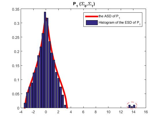
(a) Step signal $V_{1}$

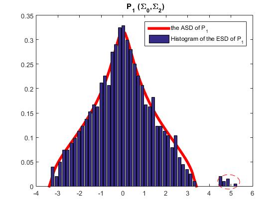
(b) Stable growth A $V_{2}$

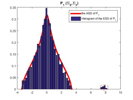
(c) Stable growth B $V_{3}$

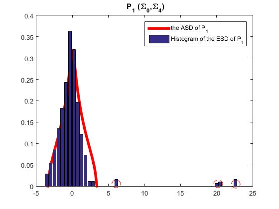
(d) Voltage collapse $V_{4}$

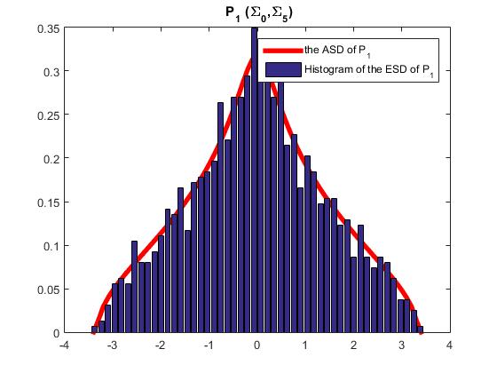
(e) White noises $V_{5}$

Figure 2: Detection results with the multivariate linear polynomial $P_{1}$

TABLE II: The values of $s$ in $\textbf{C}_{1}$–$\textbf{C}_{5}$

Cross Section	Description	$s$
$\textbf{C}_{1}$	Existence of a step signal	0.1096
$\textbf{C}_{2}$	Steady load growth	0.0357
$\textbf{C}_{3}$	Steady load growth	0.0609
$\textbf{C}_{4}$	Chaos due to voltage collapse	0.4219
$\textbf{C}_{5}$	No signa	0.000

V-B Case 2: Anomaly Detection with the Multivariate Nonlinear Polynomial $P_{2}$

In Case 2, the process is similar to V-A except that the test statistic function is replaced with

$${P_{2}}({\Sigma_{0}},{\Sigma_{i}})=({\Sigma_{i}}-{\Sigma_{0}})^{2},~{}i=1,2,3,4,5$$

which is a multivariate nonlinear polynomial in two matrices. This is the simplest second-order polynomial. Of course, we can study higher orders that will be left for the work in a next paper.

Fig. 3 shows the results. The red curve represents the ASD of ${P_{2}}$ obtained through the method in IV-B. The values of $s$ in $\textbf{C}_{1}$–$\textbf{C}_{5}$ are presented in Tab. III.

1) For Fig. 3e, the histogram agrees perfectly with the theoretical curve when in the absence of spikes; for other figures (a)-(d), there exist outliers.

2) Sort by the values of $s$: $0=\textbf{C}_{5}<\textbf{C}_{2}<\textbf{C}_{3}\ll\textbf{C}_{1}\ll\textbf{C}_{4}$.

Result 2) show that the step signals and the ramp signals are remarkably distinguished by the size of outliers. This implies that the nonlinear polynomial ${P_{2}}$ is more sensitive to outliers for the same signal-to-noise ratio, compared with its linear case. Furthermore, these results indicate that the anomaly’s influence on the grid can be estimated quantitatively by the sizes of outliers.

Compared with linearity, nonlinearity is more flexible in problem modeling and closer to the reality. Some other multivariate nonlinear polynomials may be more effective for the power grid with special load characteristics. The search for such an optimal nonlinear polynomial is beyond the scope of this paper.

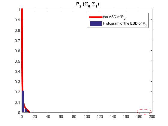
(a) Step signal $V_{1}$

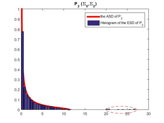
(b) Stable growth A $V_{2}$

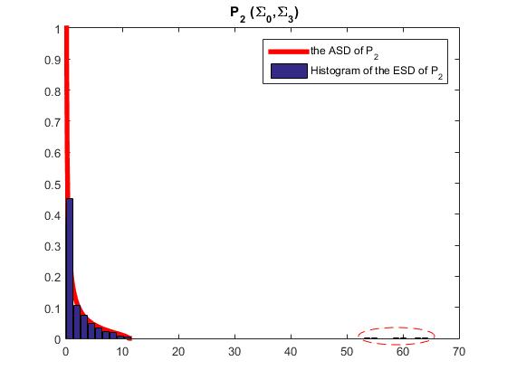
(c) Stable growth B $V_{3}$

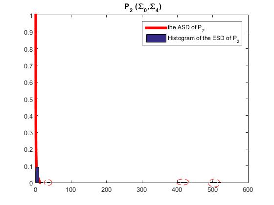
(d) Voltage collapse $V_{4}$

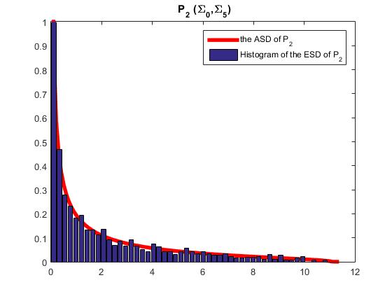
(e) White noises $V_{5}$

Figure 3: Detection results with the multivariate nonlinear polynomial $P_{2}$

TABLE III: The values of $s$ in $\textbf{C}_{1}$–$\textbf{C}_{5}$

Cross Section	Description	$s$
$\textbf{C}_{1}$	Existence of a step signal	0.9027
$\textbf{C}_{2}$	Steady load growth	0.1152
$\textbf{C}_{3}$	Steady load growth	0.2783
$\textbf{C}_{4}$	Chaos due to voltage collapse	5.2332
$\textbf{C}_{5}$	No signa	0.000

V-C Case 3: Fault Location with Simulation Data

In Case 3, the indicator $L_{i}$ defined in (20) is used to conduct fault locations. As introduced in III-B, the proposed fault location method defined in (22) is based on the hypothesis testing. Case 1 and Case 2 validate our proposed detection method and show that the nonlinear polynomial $P_{2}$ is more effective than the linear one $P_{1}.$ Thus, $P_{2}$ is selected as the test statistics in this case.

Fig. 4 is the 3D Plot for the time series of the indicator $L_{i}.$ Figures 4a, 4c and 4c show that the proposed indicator $L_{i}$ captures the bus information that is most affected by the topology change, and the location results are consistent with the the event description in Table I. The fault location fails in Fig. 4d due to voltage collapse. This result is close to the real fact.

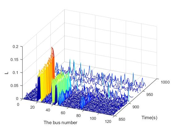
(a) Existence of a step signal for Bus 22

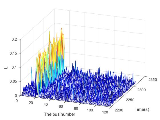
(b) Steady load growth for Bus 22

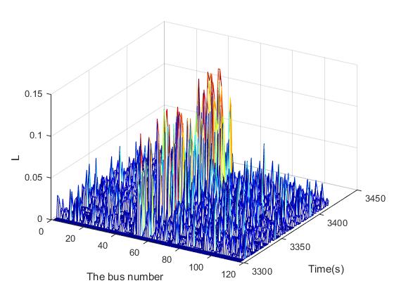
(c) Steady load growth for Bus 52

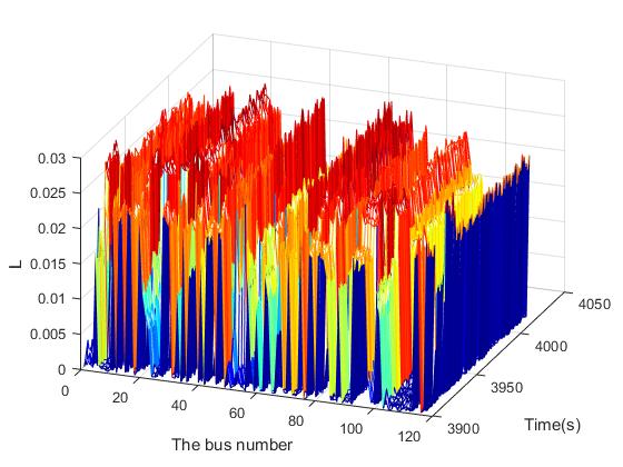
(d) Voltage collapse

Figure 4: Fault location results using the proposed method in III-B.

Fig. 5 is the result obtained by Lim’s method in [14]. The location results are close to our method at most time points. However, in some points, it is not easy to determine which bus is the most vulnerable to the load variation, especially in Fig. 5a and 5c. The reason is that the peaks in other buses are not independent of the statistic information corresponding to the largest singular value.

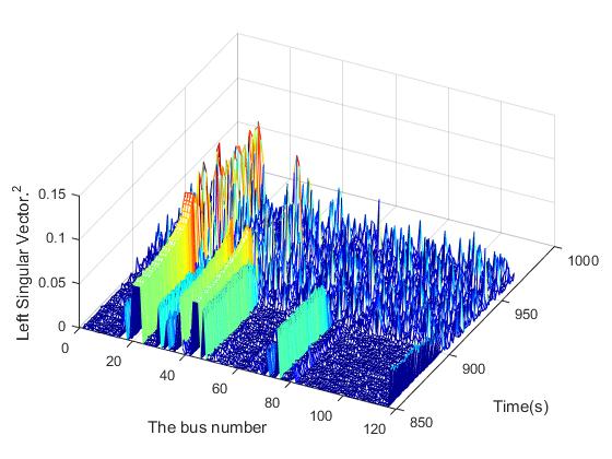
(a) Existence of a step signal for Bus 22

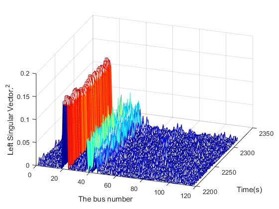
(b) Steady load growth for Bus 22

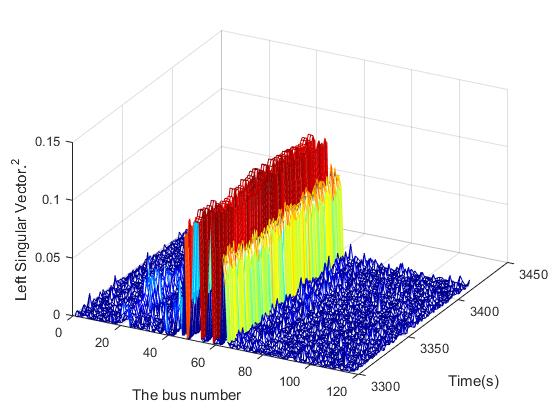
(c) Steady load growth for Bus 52

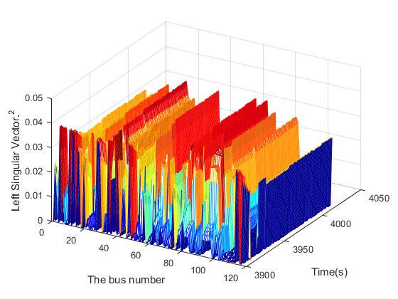
(d) Voltage collapse

Figure 5: Fault location results only using the largest singular value’s corresponding left singular vector

The reason why our method performs better is given by studying the distribution of the corresponding eigenvectors. We select the cross section $\textbf{C}_{1}$ as an example. Let $v_{ik}$ denote the $i$-th component of the eigenvector corresponding to the eigenvalue $\lambda_{k}$. Then, we normalize it such that $\sum\limits_{i=1}^{N}{v_{ik}^{2}}=N$. For a fixed $k$, the distribution of $\mu=v_{ik}$ is denoted by $p(\mu)$. The distribution of $\mu$ is plotted in Fig. 6 by dashed lines. The red solid line represents the standard normal distribution. As shown in Fig. 6a, the $p(\mu)$ for four randomly selected eigenvalues well inside the support fits extremely well with the standard normal distribution. In some sense, there is no signal contained in these eigenvectors. On the contrary, the $p(\mu)$ for outliers is markedly different from the standard normal distribution in Fig. 6b. This means that not only the largest eigenvalue but also all other outliers contain the most statistical information about the signal. In other words, all outliers matter!

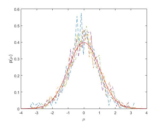
(a) Distribution of the eigenvector components of four different eigenvalues well inside the support

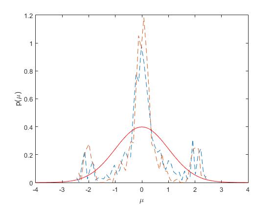
(b) Distribution of the eigenvector components of outliers

Figure 6: Distribution of the eigenvector components; the red solid line represents the standard normal distribution

V-D Case 4: Fault Location with Real 34-PMU Data

In this subsection, we evaluate the fault location indicator $L_{i}$ with real-world 34-PMU data. The real power data is a chain-reaction fault that happened in 2013 in one large power grid in China. The sample rate is 50 Hz and the total sample time is $284$ seconds (s). Fig. LABEL:34-PMU_powerflow and Fig. LABEL:34-PMU_chain-reaction illustrate the three-dimensional power flow at the whole time and the fault time respectively. The chain-reaction fault starts at $t=65.4$s.

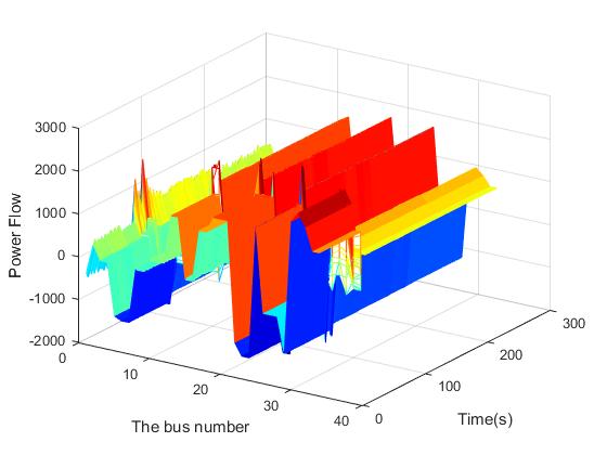
(a) The realistic 34-PMU power flow.

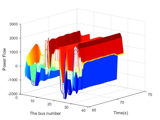
(b) The realistic 34-PMU power flow around the chain-reaction fault occurrence.

Figure 7: 3D Plot for time series of the 34-PMU power flow

Similarly to the data processing in simulation Case 3, set the sample dimension $N=34$ and the sample length $T=N$. The location of the most sensitive bus can be determined using $L_{i}$ defined in (20), using the method of (22). The result shown in Fig. 8 illustrates that the 18-th PMU ($X=18$) is the most sensitive one which is in agreement with the actual accident situation. This case validates the proposed method in real-life grid.

\begin{overpic}[scale={0.35}]{34PMU_location.jpg} \end{overpic}

Figure 8: Fault location result with the 34-PMU data

VI The estimation of the signal strength

Here we estimate the signal strength under the linear assumption:

$$V=A+N$$ (23)

where $V$ is the grid data matrix, $N$ is the noise matrix and $A$ represents the signal. Let $V_{(n,i)}$ denotes the $i$-th $n\times n$ sampling matrix and $V_{i}=N_{n,i}+A_{n,i}$. Define the matrix product as

$${M_{i}}:=V_{0}V_{i}=N_{0}(N_{i}+A_{i})$$ (24)

where $i\geq 1$.

It is natural to wonder how close the eigenvalues of $M_{i}$ are to those of $A_{i}$.

Theorem VI.1 ([23]).

Let $m\geq 1$ be an integer, and assume $\xi_{1},...,\xi_{m}$ are complex-valued random variables. For each $n\geq 1$, let $N_{n,1},...,N_{n,m}$ be an $n\times n$ i.i.d random matrix with atom variable $\xi_{1},...,\xi_{m}$, respectively. In addition, for each $1\leq k\leq m$, let $A_{n,k}$ be a deterministic $n\times n$ matrix with rank $\rm O(1)$ and operator norm $\rm O(1)$. Define the products

$${M_{n}}:=\prod\limits_{k=1}^{m}{(\frac{1}{{\sqrt{n}}}{N_{n,k}}+{A_{n,k}})},A_{n}:=\prod\limits_{k=1}^{m}{{A_{n,k}}}$$ (25)

and $\sigma:=\sigma_{1}\cdot\cdot\cdot\sigma_{m}$. Let $\varepsilon>0$, and suppose that for all sufficiently large $n$, there are no eigenvalues of $A_{n}$ in the band $\{z\in\mathbb{C}:\sigma+\varepsilon<|z|<\sigma+3\varepsilon\}$, and there are $j$ eigenvalues $\lambda_{1}(M_{n}),...,\lambda_{1}(M_{n})$ of the product $P_{n}$ in the region $\{z\in\mathbb{C}:|z|\geq\sigma+2\varepsilon\}$, and after labeling these eigenvalues properly,

$$\lambda{}_{i}({M_{n}})=\lambda{}_{i}({A_{n}})+o(1)$$ (26)

as $n\longrightarrow\infty$ for each $1\leq i\leq j$.

Theorem VI.1 reveals two main points:

1. when the sizes of matrices are large, the cross terms in (25) can be negligible outliers exit if signals exist in the system.

2. the combined strength of the signals can be bounded according to (26).

The outliers of $M_{n}$ are asymptotically close to the outliers of the product $A_{n}$ defined in (25). This implies that the combined signal strength can be estimated by calculating the eigenvalues of $M_{i}$ directly. In practice, the $M_{i}$ can be obtained by measurements but the $A_{n}$ is difficult to know.

We illustrate our approach using the simulated data used in Section V. The eigenvalues of $V_{0}V_{i},i=1,2,3,4,5$ are plotted in Fig 9, respectively.

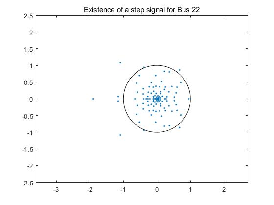
(a) Step signal $V_{1}$

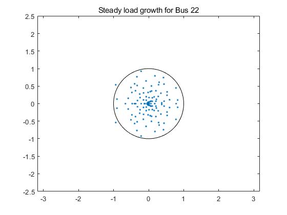
(b) Stable growth A $V_{2}$

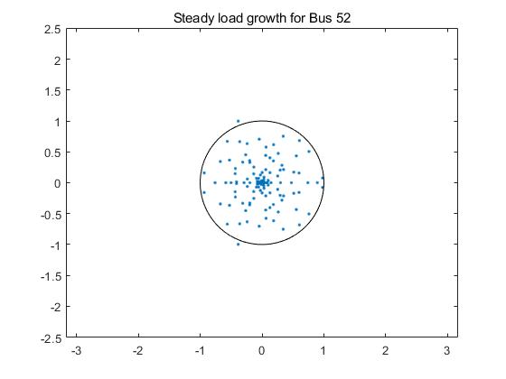
(c) Stable growth B $V_{3}$

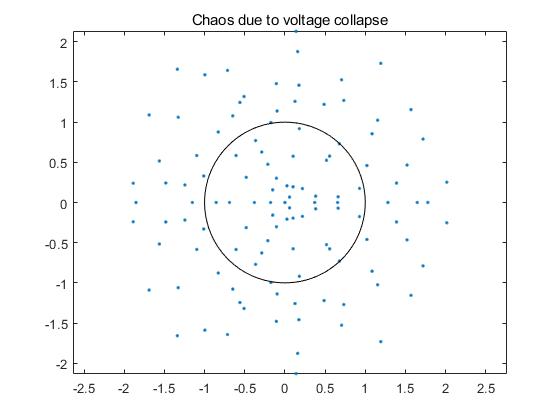
(d) Voltage collapse $V_{4}$

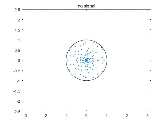
(e) White noises $V_{5}$

Figure 9: The eigenvalues of $V_{0}V_{i}$

The results in Fig 9 show an interesting phenomenon of products of random matrices: outliers appear only in the presence of the signals.

VII CONCLUSION

Built upon random matrix theory (RMT), we obtain new statistical models using massive datasets across the power grid. In this paper, we take advantage of a breakthrough by [12, 11] in free probability to calculate the asymptotic spectrum distribution of the self-adjoint matrix polynomials. Our problem of anomaly detection is formulated in terms of hypothesis testing. Fault location is also conducted. The new approach has advantages over previous ones. The results generated from the 2383-bus system agree with the asymptotic theory much better than those the 118-bus system.

As a starting point, this paper considers only two simplest examples of the self-adjoint matrix polynomials: ${P_{1}}({\Sigma_{0}},{\Sigma_{1}})={\Sigma_{1}}-{\Sigma_{0}}$ and ${P_{2}}({\Sigma_{0}},{\Sigma_{1}})={({\Sigma_{1}}-{\Sigma_{0}})^{2}},$ where ${\Sigma_{0}}$ and ${\Sigma_{1}}$ are the large-dimensional sample covariance matrices, respectively, for the null and alternative hypotheses. This problem is related to the difference between two mixed quantum states (e.g., Wishart matrices with fixed trace) [24, 25, 26] where analysis is conducted by free probability. Specifically, if we define the mixed quantum states as ${\rho_{0}}={\Sigma_{0}}/\operatorname{Tr}\left({{\Sigma_{0}}}\right),{\rho_{1}}={\Sigma_{1}}/\operatorname{Tr}\left({{\Sigma_{1}}}\right),$ we can study the difference $p{\rho_{1}}-q{\rho_{0}},{\text{ for }}p,q\in\mathbb{R},$ following [24].

Different trace functions as done in [25] can be considered in the future. Specifically, we consider the linear eigenvalue statistics (LES) of the difference of the two quantum states $\operatorname{Tr}f\left({{\rho_{1}}-{\rho_{0}}}\right)=\sum\limits_{i=1}^{n}{f\left({{\lambda_{i}}}\right)},$ where $f:\mathbb{R}\to\mathbb{R}$ is an arbitrary function of some certain smooth properties and ${{\lambda_{i}}},i=1,...,n$ is the $i-$th eigenvalue of the difference ${{\rho_{1}}-{\rho_{0}}}.$ This is the extension of the LES for one single random matrix in [9]. What is the optimal function $f$?

The algorithm of [12, 11] is very general. The techniques in quantum information theory, e.g., [24, 25, 26], have more explicit expressions to give use more transparent solutions to our problems at hand. All these papers are unified within the paradigm of free probability, a fast growing branch of random matrix theory. Note that the first use of RMT in a large power grid was by the same authors of this paper in [4]. The whole paradigm of using RMT allows one to exploit the theory of asymptotically large random matrices. The whole framework lies in the empirical observation that the asymptotic limits are very close to that finite-size random matrices, even for moderate sizes! The empirical success of using the asymptotic theory of [12, 11] in finite-size cases of our studies in a power grid will pave the way for studies of big data data analytics using other massive datasets collected in such as internet of things (IOT).

In this paper, the simple white noise representations are adopted to model the stochastic variation in load; some recent studies have adopted Ornstein-Uhlenbeck process [27] - Validation of the Ornstein-Uhlenbeck process for load modeling based on PMU measurements. These inspire us to adopt some achievements about Ornstein-Uhlenbeck Process based on RMT in the future work.

Appendix A The Specific Procedures of calculating The ASD of $P_{2}$

The following steps give the precise statement of the algorithm in  IV-B .

1. Compute the linearization of $P_{2}$

   $${{L}_{P_{2}}}={c}\otimes 1+{{b}_{0}}\otimes{{\Sigma}_{0}}+{{b}_{1}}\otimes{{\Sigma}_{1}}$$

   through Anderson’s linearization trick.

2. Compute the Cauchy transform ${{G}_{{{b}_{j}}\otimes{{\Sigma}_{j}}}}(b)$ through the scalar-valued Cauchy transforms :

   $${{G}_{{{b}_{j}}\otimes{{\Sigma}_{j}}}}(b)=\underset{\varepsilon\to 0}{\mathop{\lim}}\,-\frac{1}{\pi}\int_{\mathbb{R}}{(b-t{{b}_{j}}}{{)}^{-1}}\Im({{G}_{{{\Sigma}_{j}}}}(t+i\varepsilon))dt.$$

   for $j=0,1$.

3. Calculate the Cauchy transform of

   $${{L}_{P_{2}}}-{c}\otimes 1={{b}_{0}}\otimes{{\Sigma}_{0}}+{{b}_{1}}\otimes{{\Sigma}_{1}}$$

   by applying Theorem IV.1. The Cauchy transform of ${{L}_{P_{2}}}$ is then given by

   $${{G}_{{{L}_{P_{2}}}}}(b)={{G}_{{{L}_{P_{2}}}-{c}\otimes 1}}(b-{c}).$$

4. According to Corollary IV.3, the scalar-valued Cauchy transform ${{G}_{P_{2}}}(z)$ of $P_{2}$ is obtained by

   $${{G}_{P_{2}}}(z)\text{=}\underset{\varepsilon\to\text{0}}{\mathop{\lim}}\,{{\left[G{}_{{{L}_{P_{2}}}}({{\Lambda}_{\varepsilon}}(z))\right]}_{1,1}}\quad for\;all\;z\in{{\mathbb{C}}^{+}}.$$

5. Compute the distribution of $P_{2}$ via the Stieltjes inversion formula.

Appendix B The standard IEEE 118-bus system and The load variation

\begin{overpic}[scale={0.2}]{IEEE118-eps-converted-to} \end{overpic}

Figure 10: The network structure for the IEEE 118-bus system.

\begin{overpic}[scale={0.2}]{V230_loadhx} \par\end{overpic}

Figure 11: The event assumptions on time series.

Appendix C The 2383-Bus case

For simplicity, the signals for each bus are shown in Tab. IV. The detection results, the values of $s$ location results are shown in Fig.12, Tab.V and Fig. 13 respectively. The results generated from the 2383-bus system are the same as the 118-bus system.

TABLE IV: Descriptions of the 2383-bus system status

Bus	Duration(s)	Descripiton
59	3100 $\sim$ 3200	Steady load growth
	5100	Existence of a step signal
	6000 $\sim$ 6100	Chaos due to voltage collapse
Others	1 $\sim$ 10000	No signal

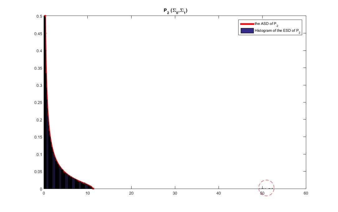
(a) Steady load growth for Bus 59

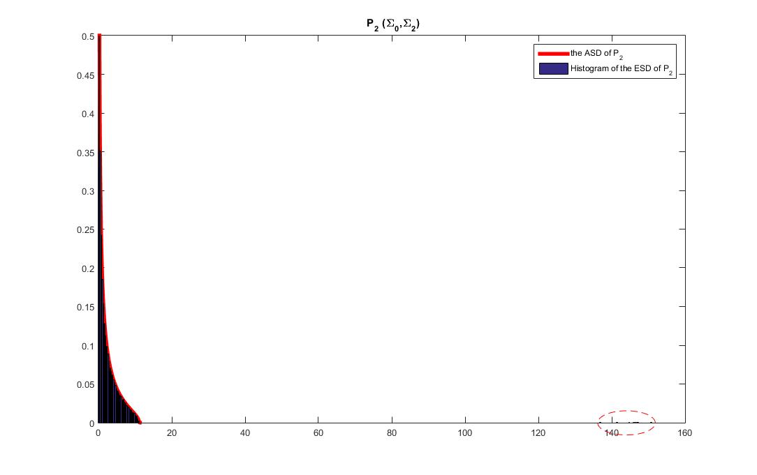
(b) Existence of a step signal for Bus 59

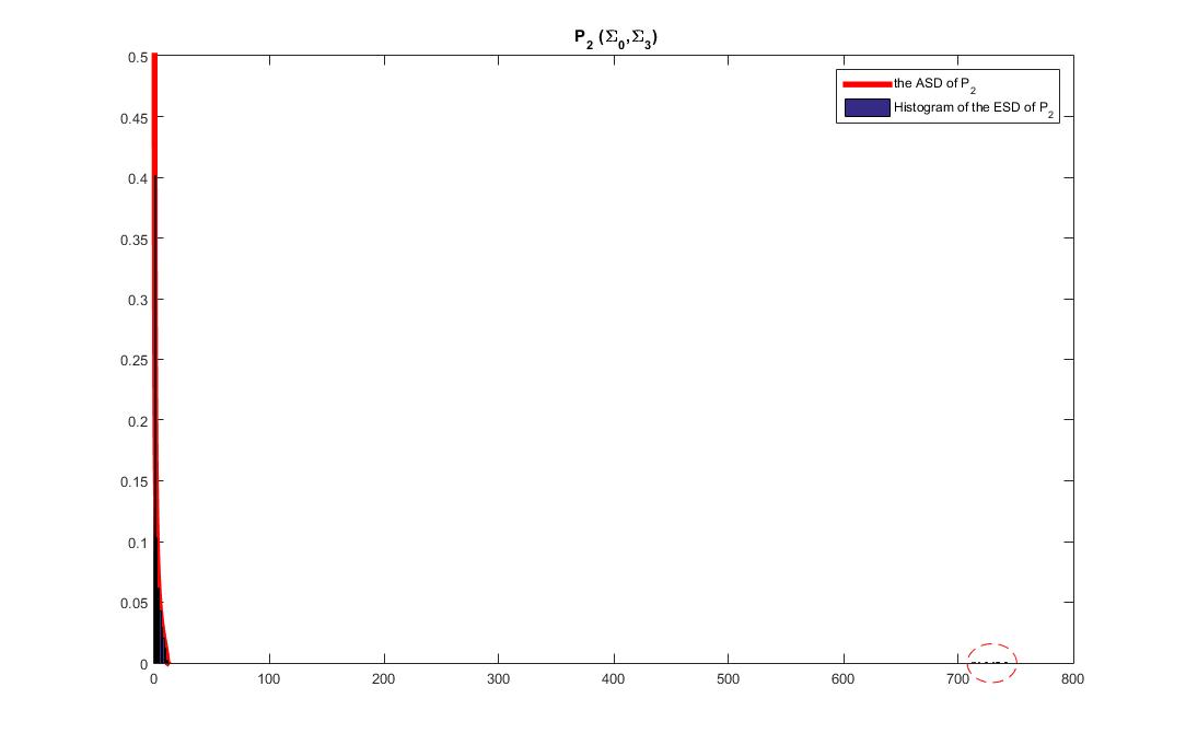
(c) Voltage collapse

Figure 12: Detection results of the 2383-bus case

TABLE V: The values of $s$

Durations	Description	$s$
3100 $\sim$ 3200	Steady load growth	0.2538
5100	Existence of a step signal	2.045
6000 $\sim$ 6100	Chaos due to voltage collapse	9.668

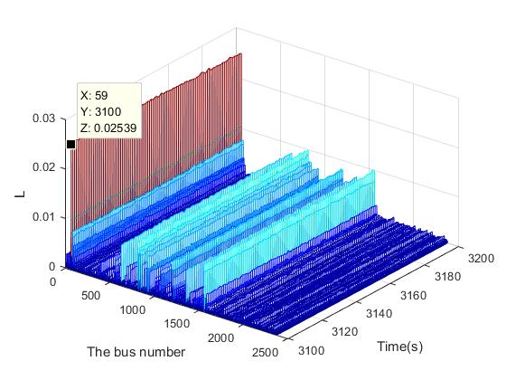
(a) Steady load growth for Bus 59

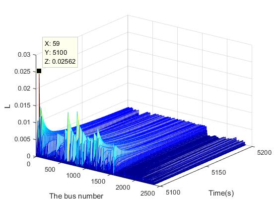
(b) Existence of a step signal for Bus 59

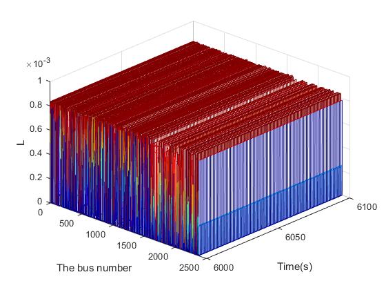
(c) Voltage collapse

Figure 13: Fault location results of the 2383-bus case

References

- [1] T. Hong, C. Chen, J. Huang, N. Lu, L. Xie, and H. Zareipour, “Guest editorial big data analytics for grid modernization,” IEEE Transactions on Smart Grid, vol. 7, no. 5, pp. 2395–2396, Sept 2016.
- [2] C. Lu, B. Shi, X. Wu, and H. Sun, “Advancing china? s smart grid: Phasor measurement units in a wide-area management system,” IEEE Power and Energy Magazine, vol. 13, no. 5, pp. 60–71, 2015.
- [3] S. Nuthalapati and A. G. Phadke, “Managing the grid: Using synchrophasor technology [guest editorial],” IEEE Power and Energy Magazine, vol. 13, no. 5, pp. 10–12, 2015.
- [4] X. He, Q. Ai, R. C. Qiu, W. Huang, L. Piao, and H. Liu, “A big data architecture design for smart grids based on random matrix theory,” IEEE transactions on smart Grid, vol. 32, no. 5, 2015.
- [5] R. Qiu and P. Antonik, Smart Grid Using Big Data Analytics–A Random Matrix Theory Approach. John Wiley and Sons, 2016, 600 pages.
- [6] R. Qiu and M. Wicks, Cognitive Networked Sensing and Big Data. Springer, 2013.
- [7] J. M. Lim and C. L. DeMarco, “Svd-based voltage stability assessment from phasor measurement unit data,” IEEE Transactions on Power Systems, vol. PP, no. 99, pp. 1–9, 2015.
- [8] X. Xu, X. He, Q. Ai, and R. Qiu, “A correlation analysis method for power systems based on random matrix theory,” IEEE Trans. Smart Grid, vol. 8, no. 4, pp. 1811–1820, 2017.
- [9] X. He, R. C. Qiu, Q. Ai, L. Chu, X. Xu, and Z. Ling, “Designing for situation awareness of future power grids: An indicator system based on linear eigenvalue statistics of large random matrices,” IEEE Access, vol. 4, pp. 3557–3568, 2016.
- [10] L. Chu, R. C. Qiu, X. He, Z. Ling, and Y. Liu, “Massive streaming pmu data modeling and analytics in smart grid state evaluation based on multiple high-dimensional covariance tests,” IEEE Transactions on Big Data, vol. PP, no. 99, pp. 1–1, 2016.
- [11] S. Belinschi, T. Mai, and R. Speicher, “Analytic subordination theory of operator-valued free additive convolution and the solution of a general random matrix problem,” Journal F r Die Reine Und Angewandte Mathematik, 2013.
- [12] R. Speicher and R. Speicher, “Polynomials in asymptotically free random matrices,” Acta Physica Polonica, vol. 46, no. 9, 2015.
- [13] Y. Chen, L. Xie, and P. Kumar, “Dimensionality reduction and early event detection using online synchrophasor data,” in Power and Energy Society General Meeting (PES), 2013 IEEE. Vancouver, BC: IEEE, July 2013, pp. 1–5.
- [14] J. M. Lim and C. L. Demarco, “Model-free voltage stability assessments via singular value analysis of pmu data,” 2013, pp. 1–10.
- [15] L. Xie, Y. Chen, and P. Kumar, “Dimensionality reduction of synchrophasor data for early event detection: Linearized analysis,” Power Systems, IEEE Transactions on, vol. 29, no. 6, pp. 2784–2794, 2014.
- [16] D. M. Eltigani, K. Ramadan, and E. Zakaria, “Implementation of transient stability assessment using artificial neural networks,” in International Conference on Computing, Electrical and Electronics Engineering, 2013, pp. 659–662.
- [17] D. Q. Zhou, U. D. Annakkage, and A. D. Rajapakse, “Online monitoring of voltage stability margin using an artificial neural network,” IEEE Transactions on Power Systems, vol. 25, no. 3, pp. 1566–1574, 2010.
- [18] V. A. Marchenko and L. A. Pastur, “Distribution of eigenvalues for some sets of random matrices,” Mathematics of the USSR-Sbornik, vol. 1, no. 1, p. 507–536, 1967.
- [19] Loubaton, Philippe, and Vallet, “Almost sure localization of the eigenvalues in a gaussian information plus noise model. applications to the spiked models,” vol. 16, no. 24, pp. 1934–1959, 2011.
- [20] J. Pielaszkiewicz and M. Singull, “Closed form of the asymptotic spectral distribution of random matrices using free independence,” 2015.
- [21] G. W. Anderson, “Convergence of the largest singular value of a polynomial in independent wigner matrices,” Annals of Probability, vol. 38, no. 1, p. 110 C112, 2011.
- [22] R. D. Zimmerman and C. E. Murillo-S nchez, “Matpower 4.1 user’s manual,” Power Systems Engineering Research Center, 2011.
- [23] N. Coston, S. O’Rourke, and P. M. Wood, “Outliers in the spectrum for products of independent random matrices,” 2017.
- [24] J. Mejía, C. Zapata, and A. Botero, “The difference between two random mixed quantum states: exact and asymptotic spectral analysis,” Journal of Physics A: Mathematical and Theoretical, vol. 50, no. 2, p. 025301, 2016.
- [25] Z. Puchała, Ł. Pawela, and K. Życzkowski, “Distinguishability of generic quantum states,” Physical Review A, vol. 93, no. 6, p. 062112, 2016.
- [26] I. Nechita, Z. Puchała, Ł. Pawela, and K. Życzkowski, “Almost all quantum channels are equidistant,” arXiv preprint arXiv:1612.00401, 2016.
- [27] C. Roberts, E. M. Stewart, and F. Milano, “Validation of the ornstein-uhlenbeck process for load modeling based on pmu measurements,” in Power Systems Computation Conference, 2016.