On the maximum of discretely sampled fractional Brownian motion with small Hurst parameter

Abstract

We show that the distribution of the maximum of the fractional Brownian motion $B^{H}$ with Hurst parameter $H\to 0$ over an $n$-point set $\tau\subset[0,1]$ can be approximated by the normal law with mean $\sqrt{\ln n}$ and variance $1/2$ provided that $n\to\infty$ slowly enough and the points in $\tau$ are not too close to each other.

Key words and phrases: fractional Brownian motion, maxima, discrete sampling, normal approximation.

AMS Subject Classification: 60G22, 60G15, 60E15, 60F05.

1 Introduction

Let $\{B^{H}_{t}\}_{t\geq 0}$ be the fractional Brownian motion (fBM) with Hurst index $H\in(0,1]$. Recall that the fBM is a zero-mean continuous Gaussian process with the covariance function

$${\bf E}B^{H}_{s}B^{H}_{t}=\frac{1}{2}\bigl{(}s^{2H}+t^{2H}-|t-s|^{2H}\bigr{)},\quad s,t\geq 0.$$

Alternatively, $B^{H}$ can be defined as a continuous Gaussian process with stationary increments such that $B_{t}^{H}$ has zero mean and variance $t^{2H}$. In particular, $W:=B^{1/2}$ is the standard Brownian motion (BM) that has independent increments. The increments of $B^{H}$ are positively correlated if $H>1/2$ and negatively correlated if $H<1/2$.

The fBM has found use in many models in applied fields (see, e.g., the survey in the preface to the monograph [7]). In particular, the processes $B^{H}$ with small $H$ (the case we are focussing on in this paper) have recently been used to model stock price volatility [5, 1]. It is interesting and important for a number of applications to know the distribution (or a suitable approximation thereof) of the maximum

$$\overline{B^{H}_{T}}:=\max_{0\leq t\leq T}B^{H}_{t}$$

of the fBM on a fixed time interval $[0,T]$, $T>0.$ Unfortunately, besides the case of the standard BM ($H=1/2$) and the degenerate case $H=1$ (where $B_{t}^{1}=\zeta t,$ $t\geq 0,$ for a standard normal random variable $\zeta$), there is no known closed form expression for the distribution of $\overline{B_{T}^{H}}.$ As in practice one usually deals with discretely sampled data, what would be of real practical interest is actually the behavior of the distribution of the maximum of the fBM sampled on a discrete time grid on $[0,T]$.

In this paper, we consider the case when $H$ vanishes and deal with the maxima of the fBM $B^{H}$ sampled on a (generally speaking, non-uniform) discrete time grid. Recall that in that case the finite-dimensional distributions of $B^{H}$ converge to those of a “translated” continuum of independent normal random variables (see, e.g., [2]):

$$\{B^{H}\}_{t\geq 0}\stackrel{{\scriptstyle\text{f.d.d.}}}{{\longrightarrow}}\{\xi\}_{t\geq 0}\quad\mbox{as}\quad H\to 0,$$ (1)

where $\xi_{t}:=(\zeta_{t}-\zeta_{0})/\sqrt{2},$ $\{\zeta_{t}\}_{t\geq 0}$ is a family of independent standard normal random variables. It is clear from (1) that $\overline{B^{H}_{T}}\stackrel{{\scriptstyle P}}{{\longrightarrow}}\infty$ as $H\to 0$. However, for any fixed finite subset

$$\tau=\{t_{i}\}_{i=1}^{n}\subset[0,T],\quad\mbox{where}\ t_{1}<t_{2}<\cdots<t_{n},$$ (2)

if one considers the random vector

$$B^{H,\tau}:=(B^{H}_{t_{1}},B^{H}_{t_{2}},\ldots,B^{H}_{t_{n}})\in\mathbb{R}^{n},$$

and let $\overline{x}:=\max_{1\leq i\leq n}x_{i}$ for a vector $x\in\mathbb{R}^{n},$ relation (1) implies the convergence in distribution

$$\overline{B^{H,\tau}}\stackrel{{\scriptstyle d}}{{\longrightarrow}}(\overline{\zeta^{n}}-\zeta_{0})/\sqrt{2}\quad\mbox{as}\quad H\to 0,$$ (3)

where $\zeta^{n}:=(\zeta_{1},\ldots,\zeta_{n})$. One can easily see that the distribution function of the random variable on the RHS of (3) is given by the convolution $(\Phi^{n}*\Phi)(\sqrt{2}x)$, where $\Phi$ is the standard normal distribution function.

Now what can be said about the behavior of $\overline{B^{H,\tau}}$ when simultaneously $H\to 0$ and the number $n$ of points in the partition $\tau$ tends to infinity? One can conjecture that, if $n\to\infty$ slowly enough (so that the dependence between the components of the vector $B^{H,\tau}$ decays sufficiently quickly), then the distribution of $\overline{B^{H,\tau}}$ would still be close to that of the RHS of (3). The behavior of the distribution of $\overline{\zeta^{n}}$ as $n\to\infty$ has been known since the work of Fisher and Tippett [3] who demonstrated that, taking $a_{n}:=\sqrt{2\ln n}$ and $b_{n}:=\sqrt{2\ln n}-(\ln\ln n+\ln(4\pi))/(2\sqrt{2\ln n}),$ one has

$$a_{n}(\overline{\zeta^{n}}-b_{n})\stackrel{{\scriptstyle d}}{{\longrightarrow}}G\quad\mbox{as}\quad n\to\infty,$$ (4)

where the limiting random variable $G$ follows the Gumbel distribution $\Lambda(x)=e^{-e^{-x}},$ $x\in\mathbb{R}$. In fact, the uniform distance between the distribution functions of the LHS of (4) and $\Lambda$ was shown to be of the order of $1/\ln n$ [6]. Choosing slightly different sequences

$$b_{n}:=\Phi^{-1}(1-1/n),\quad a_{n}:=b_{n}+1/b_{n},$$ (5)

one can show that that distance admits an asymptotic upper bound of the form $1/(3\ln n)$ (see [4]).

So one can expect a first order approximation of the form $\sqrt{\ln n}+\zeta_{0}/\sqrt{2}$ to hold true for the maximum $\overline{B^{H,\tau}}$ as $n\to\infty$, provided that $H\to 0$ fast enough for the given decay rate of the distance between the points $t_{i}$. Our main result below confirms that conjecture and specifies conditions under which it holds. Without loss of generality, we consider the case $T=1$ only, since the case of arbitrary $T$ can be easily reduced to the former using the self-similarity property of the fBM.

2 The main result

Denote by $\stackrel{{\scriptstyle st}}{{\leq}}$ the stochastic order relation for random variables: we write $\xi\stackrel{{\scriptstyle st}}{{\leq}}\eta$ iff ${\bf P}(\xi\leq x)\geq{\bf P}(\eta\leq x)$, $x\in\mathbb{R}$, and $\xi\stackrel{{\scriptstyle st}}{{\geq}}\eta$ iff $\eta\stackrel{{\scriptstyle st}}{{\leq}}\xi$. By

$$\delta(\tau):=\min_{1\leq i\leq n}(t_{i}-t_{i-1}),\quad\mbox{where $t_{0}:=0$},$$

we denote the minimal distance between the points of the finite subset $\tau$ (cf. (2)). As usual, $o_{P}(1)$ denotes a sequence of random variables converging to zero in probability.

Theorem.

Let $H_{k}\in(0,1]$ be such that $H_{k}\to 0$ as $k\to\infty$, and $\tau_{k}=\{t_{k,i}\}_{i=1}^{n_{k}}$ be a sequence of subsets of $(0,1]$, $t_{k,1}<\cdots<t_{k,n_{k}},$ such that $n_{k}\to\infty$, $\delta_{k}:=\delta(\tau_{k}).$

(i) If $H_{k}(\ln n_{k})^{1/2}\to 0$ and $H_{k}\ln(n_{k}\delta_{k})\to 0$ as $k\to\infty$ then

$$\overline{B^{H_{k},\tau_{k}}}\stackrel{{\scriptstyle st}}{{\leq}}\sqrt{\ln n_{k}}+\zeta_{0}/\sqrt{2}+o_{P}(1).$$ (6)

(ii) If $H_{k}(\ln n_{k})^{2}\to 0$ and $H_{k}\ln\delta_{k}\to 0$ as $k\to\infty$, then

$$\overline{B^{H_{k},\tau_{k}}}\stackrel{{\scriptstyle st}}{{\geq}}\sqrt{\ln n_{k}}+\zeta_{0}/\sqrt{2}+o_{P}(1).$$

Thus, under the assumptions from part (ii), one has

$$\overline{B^{H_{k},\tau_{k}}}-\sqrt{\ln n_{k}}\stackrel{{\scriptstyle d}}{{\longrightarrow}}\zeta_{0}/\sqrt{2}\quad\mbox{as}\quad k\to\infty.$$

Note also that the conditions $H_{k}\ln(n_{k}\delta_{k})\to 0$ and $H_{k}\ln\delta_{k}\to 0$ from parts (i) and (ii), respectively, are automatically met in the case of “uniform grids” $\tau_{k}$ (when $\delta(\tau_{k})=1/n_{k}$).

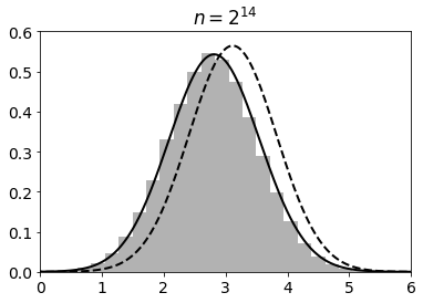
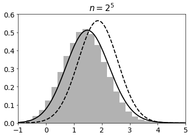
Simulations indicate that in fact, in accordance with (4), a better approximation to the law of $\overline{B^{H_{k},\tau_{k}}}$ is given by the distribution $D_{n}(x):=(\Lambda_{n}*\Phi)(\sqrt{2}x),$ the convolution being that of the scaled version of the Gumbel law $\Lambda_{n}(x)=\Lambda(a_{n}(x-b_{n}))$ with the standard normal distribution. The curves in Fig. 1 are the fitting normal density (dashed lines) and the density of $D_{n}$ (solid lines), where $a_{n},b_{n}$ were chosen according to (5), overlayed upon the histograms constructed from the respective simulations. However, establishing the validity of that second order approximation analytically is much harder than the analysis in the present note and may require more refined techniques.

Figure 1: The histograms show the empirical distributions of $\overline{B^{H,\tau}}$ for $10^{5}$ simulated paths of the fBM $B^{H}$ with the uniform partition $\tau=\{i/n\}_{1\leq i\leq n}$ and $H=(\ln n)^{-2}$. The dashed lines show the approximating normal densities, and the solid lines the approximations by the convolutions of the scaled Gumbel and normal densities.

3 The proof of the theorem

(i) Let $W$ be a standard BM process independent of $\{\zeta_{t}\}$. Set $s_{k,i}:=(t_{k,i})^{2H_{k}}$, $i=1,\ldots,n_{k}$, and introduce random vectors $X^{k},Y^{k}\in\mathbb{R}^{n_{k}}$ with the respective components

$$X^{k}_{i}:=(s_{k,i}^{1/2}\zeta_{i}-W_{s_{k,i}})/\sqrt{2},\qquad Y^{k}_{i}:=(\zeta_{i}-W_{s_{k,i}})/\sqrt{2}.$$

First we show that

$$\overline{B^{H_{k},\tau_{k}}}\stackrel{{\scriptstyle st}}{{\leq}}\overline{X^{k}},$$ (7)

then give an upper bound for $\overline{X^{k}}$ in terms of $\overline{Y^{k}},$ and finally demonstrate that that bound is of the form of the RHS of (6).

Clearly, ${\bf E}X^{k}=0$ and

$$\mbox{\rm Cov}\,(X^{k}_{i},X^{k}_{j}) =2^{-1}\bigl{(}s_{k,i}^{1/2}s_{k,j}^{1/2}\mbox{\rm Cov}\,(\zeta_{i},\zeta_{j})+\mbox{\rm Cov}\,(W_{s_{k,i}},W_{s_{k,j}})\bigr{)}$$

$$=2^{-1}\bigl{(}s_{k,i}\delta_{ij}+s_{k,i}\wedge s_{k,j})\bigr{)},\quad 1\leq i,j\leq n_{k},$$

where $\delta_{ij}$ is Kronecker’s delta. Therefore,

$${\bf E}X^{k}_{i}={\bf E}B^{H_{k},\tau_{k}}_{i},\quad\mbox{\rm Var}\,X^{k}_{i}=\mbox{\rm Var}\,B^{H_{k},\tau_{k}}_{i},\quad 1\leq i\leq n_{k},$$ (8)

and, for $1\leq i<j\leq n_{k},$ one has

$$\begin{split}\mbox{\rm Cov}\,(X^{k}_{i},X^{k}_{j})&=\mbox{$\frac{1}{2}$}s_{k,i}<\mbox{$\frac{1}{2}$}\bigl{(}s_{k.i}+s_{k,j}-s_{k,j}(1-t_{k,i}/t_{k,j})^{2H_{k}}\bigr{)}\\ &=\mbox{\rm Cov}\,(B^{H_{k},\tau_{k}}_{i},B^{H_{k},\tau_{k}}_{j}).\end{split}$$ (9)

Now (7) immediately follows from Slepian’s lemma [8].

Next let $i(k):=\mathrm{argmax}_{1\leq i\leq n_{k}}X^{k}_{i}$, which is clearly well-defined a.s. Since $s_{k,i}\leq 1,$ it is easy to see that

$$\overline{X^{k}}\leq\overline{Y^{k}}{\bf 1}(\zeta_{i(k)}\geq 0)-2^{-1/2}W_{s_{k,i(k)}}{\bf 1}(\zeta_{i(k)}<0).$$ (10)

We will now show that

$$\overline{Y^{k}}\leq\sqrt{\ln n_{k}}-W_{1}/\sqrt{2}+o_{P}(1).$$ (11)

The assumption that $H_{k}(\ln n_{k})^{1/2}\to 0$ ensures that it is possible to choose a sequence $\varepsilon_{k}>0$ such that the following relations hold as $k\to\infty$:

$$\varepsilon_{k}\to 0,\qquad m_{k}:=\varepsilon_{k}n_{k}\in\mathbb{N},$$

$$\frac{|\ln\varepsilon_{k}|}{\ln n_{k}}\to 0,\qquad\frac{|\ln\varepsilon_{k}|}{\sqrt{\ln n_{k}}}\to\infty,$$ (12)

$$m_{k}\to\infty,\qquad H_{k}|\ln\varepsilon_{k}|\to 0.$$ (13)

Indeed, one can set $\varepsilon_{k}:=e^{-N_{k}\sqrt{\ln n_{k}}}$ with a quantity $N_{k}\to\infty$ such that $N_{k}(\ln n_{k})^{1/2}=o\bigl{(}H^{-1}_{k}\wedge\ln n_{k}\bigr{)}$ (for example, $N_{k}:=(H_{k}(\ln n_{k})^{1/2})^{-1/2}\wedge(\ln n_{k})^{1/4}$, adjusted if necessary to ensure that $m_{k}\in\mathbb{N}$).

Now set $C_{k,1}:=\{i:1\leq i\leq m_{k}\}$, $C_{k,2}:=\{i:m_{k}<i\leq n_{k}\}$ and let

$$M_{k,j}:=\max_{i\in C_{k,j}}\bigl{(}\zeta_{i}-W_{s_{k,i}}\bigr{)},\quad j=1,2,$$

so that $\overline{Y^{k}}=(M_{k,1}\vee M_{k,2})/\sqrt{2}$.

To bound $M_{k,1},$ note that

$$x_{k}:=\sqrt{2\ln m_{k}}=\sqrt{2\ln n_{k}\Bigl{(}1+\frac{\ln\varepsilon_{k}}{\ln n_{k}}\Bigr{)}}\leq\sqrt{2\ln n_{k}}\Bigl{(}1+\frac{\ln\varepsilon_{k}}{2\ln n_{k}}\Bigr{)}=\sqrt{2\ln n_{k}}-2h_{k},$$

where in view of (12) one has

$$h_{k}:=|\ln\varepsilon_{k}|/(2\sqrt{2\ln n_{k}})\to\infty.$$ (14)

Using the standard Mills’ ratio bound for the normal distribution, we have

$${\bf P}(\overline{\zeta^{m_{k}}}>x_{k})\leq m_{k}{\bf P}(\zeta_{1}>x_{k})\leq\frac{m_{k}e^{-x^{2}_{k}/2}}{\sqrt{2\pi}x_{k}}=\frac{1}{\sqrt{4\pi\ln m_{k}}}\to 0$$ (15)

in view of (13). Setting $\underline{W_{1}}:=\min_{0\leq t\leq 1}W_{t}$, we obtain that

$${\bf P}(M_{k,1}>\sqrt{2\ln n_{k}}-h_{k}) \leq{\bf P}(\overline{\zeta^{m_{k}}}-\underline{W_{1}}>\sqrt{2\ln n_{k}}-h_{k})$$

$$\leq{\bf P}(\overline{\zeta^{m_{k}}}>\sqrt{2\ln n_{k}}-2h_{k})+{\bf P}(-\underline{W_{1}}>h_{k})\to 0$$ (16)

by (14) and (15).

Now we turn to the term $M_{k,2}$. As $W$ has continuous trajectories, there exist $\theta_{k}\in[s_{k,m_{k}},1]$, which depend on the trajectory of $W$, such that

$$M_{k,2}=\max_{m_{k}<i\leq n_{k}}\zeta_{i}-W_{\theta_{k}}\leq\overline{\zeta^{n_{k}}}-W_{1}+o_{P}(1),$$ (17)

where the last relation holds as $W_{\theta_{k}}\to W_{1}$ because $\theta_{k}\to 1$ since

$$s_{k,m_{k}}\geq(m_{k}\delta_{k})^{2H_{k}}=\varepsilon_{k}^{2H_{k}}(n_{k}\delta_{k})^{2H_{k}}\to 1$$ (18)

due to the assumption that $H_{k}\ln(n_{k}\delta_{k})\to 0$ and (13).

Since $\overline{\zeta^{n_{k}}}=\sqrt{2\ln n_{k}}+o_{P}(1)$ in view of (4), from (16) and (17) we obtain that $M_{k,1}\vee M_{k,2}\leq\sqrt{2\ln n_{k}}-W_{1}+o_{P}(1)$, which proves (11).

Now observe that obviously

$$-W_{s_{k,i(k)}}\leq\sqrt{2\ln n_{k}}-W_{1}+o_{P}(1)$$

and $W_{1}\stackrel{{\scriptstyle d}}{{=}}-\zeta_{0}$. That, together with (7), (10) and (11), completes the proof of part (i) of the theorem.

(ii) Consider the differences

$$d_{k,ij}:=\bigl{(}\mbox{\rm Cov}\,B^{H_{k},\tau_{k}}-\mbox{\rm Cov}\,X^{k}\bigr{)}_{ij}\geq 0,\quad 1\leq i,j\leq n_{k}$$

(cf. (8), (9)). Note that $d_{k,ii}=0,$ $1\leq i\leq n_{k},$ by (8), and that for $i<j$ one has

$$d_{k,ij} =\frac{1}{2}\biggl{[}\Bigl{(}\frac{j}{n_{k}}\Bigr{)}^{2H_{k}}-\Bigl{(}\frac{j-i}{n_{k}}\Bigr{)}^{2H_{k}}\biggr{]}\leq\frac{1}{2}\biggl{[}1-\Bigl{(}\frac{1}{n_{k}}\Bigr{)}^{2H_{k}}\biggr{]}\leq H_{k}\ln n_{k}:=q_{k}$$

since $1-1/x\leq\ln x$ for all $x>0$. Denoting by $I_{k}:=(\delta_{ij})$ and $J_{k}:=(1)$ the unit and all-ones $(n_{k}\times n_{k})$-matrices, respectively, we conclude that

$$(\mbox{\rm Cov}\,B^{H_{k},\tau_{k}}+q_{k}I_{k})_{ij}\leq(\mbox{\rm Cov}\,X^{k}+q_{k}J_{k})_{ij},\quad 1\leq i,j\leq n_{k},$$ (19)

with equalities holding for $i=j$.

On the LHS of (19) we have got the entries of the covariance matrix of the random vector $B^{H_{k},\tau_{k}}+q_{k}^{1/2}\zeta^{n_{k}}$ (assuming that $\{\zeta_{t}\}$ is independent of $B^{H_{k}}$), whereas on the RHS are those for the vector $X^{k}+q_{k}^{1/2}\zeta_{0}$ (addition with a scalar is understood in the component-wise sense). Since the means of those random vectors are zeros, by Slepian’s lemma one has

$$\overline{B^{H_{k},\tau_{k}}+q_{k}^{1/2}\zeta^{n_{k}}}\stackrel{{\scriptstyle st}}{{\geq}}\overline{X^{k}+q_{k}^{1/2}\zeta_{0}}=\overline{X^{k}}+q_{k}^{1/2}\zeta_{0}=\overline{X^{k}}+o_{P}(1).$$

Using (4), we have

$$q_{k}^{1/2}\overline{\zeta^{n_{k}}}=q_{k}^{1/2}\sqrt{2\ln n_{k}}+o_{P}(1)=o_{P}(1)$$

as $q_{k}\ln n_{k}=H_{k}(\ln n_{k})^{2}=o(1)$ by assumption. Hence, by the lemma from the Appendix, one has

$$\overline{B^{H_{k},\tau_{k}}}\geq\overline{B^{H_{k},\tau_{k}}+q_{k}^{1/2}\zeta^{n_{k}}}-q_{k}^{1/2}\overline{\zeta^{n_{k}}}\stackrel{{\scriptstyle st}}{{\geq}}\overline{X^{k}}+o_{P}(1).$$ (20)

On the event $A_{k}=\{\max_{m_{k}<i\leq n_{k}}\zeta_{i}\geq 0\}$ we have

$$2^{1/2}\overline{X^{k}}\geq\max_{m_{k}<i\leq n_{k}}\bigl{(}s_{k,i}^{1/2}\zeta_{i}-W_{s_{k,i}}\bigr{)}\geq s_{k,m_{k}}^{1/2}\max_{m_{k}<i\leq n_{k}}\zeta_{i}+\min_{s_{k,m_{k}}\leq t\leq 1}W_{t}.$$

In view of the first two relations in (18), the second relation in (13) and the assumption of part (ii) of the theorem, we have $s_{k,m_{k}}\to 1$ as $k\to\infty.$ Therefore,

$$\min_{s_{k,m_{k}}\leq t\leq 1}W_{t}\stackrel{{\scriptstyle d}}{{=}}\zeta_{0}+o_{P}(1).$$

Since clearly ${\bf P}(A_{k})\to 1,$ we obtain that

$$2^{1/2}\overline{X^{k}}\stackrel{{\scriptstyle st}}{{\geq}}s_{k,m_{k}}^{1/2}\max_{m_{k}<i\leq n_{k}}\zeta_{i}+\zeta_{0}+o_{P}(1).$$

For the first term on the RHS, using (4), one has

$$\max_{m_{k}<i\leq n_{k}}\zeta_{i}\stackrel{{\scriptstyle d}}{{=}}\overline{\zeta^{(1-\varepsilon_{k})n_{k}}}=\sqrt{2\ln((1-\varepsilon_{k})n_{k})}+o_{P}(1)=\sqrt{2\ln n_{k}}+o_{P}(1)$$

as clearly $\varepsilon_{k}\sqrt{\ln n_{k}}=o(1)$. Thus, $\overline{X^{k}}\stackrel{{\scriptstyle st}}{{\geq}}\sqrt{\ln n_{k}}+\zeta_{0}/\sqrt{2}+o_{P}(1)$. To complete the proof of part (ii) of the theorem, it remains to combine the last bound with (20) and again use the lemma from the Appendix.

Appendix

The following simple lemma was used in the proof of the theorem.

Lemma.

Suppose $X,Y$ are two random variables such that $X$ has a continuous distribution and $X\stackrel{{\scriptstyle st}}{{\geq}}Y$, while $Z$ is a random variable defined on the same probability space as $X$. Then there exist random variables $Y^{\prime},Z^{\prime}$ such that $X+Z\stackrel{{\scriptstyle st}}{{\geq}}Y^{\prime}+Z^{\prime}$ and $Y\stackrel{{\scriptstyle d}}{{=}}Y^{\prime}$, $Z\stackrel{{\scriptstyle d}}{{=}}Z^{\prime}$.

In particular, if $X_{n}\stackrel{{\scriptstyle st}}{{\geq}}Y_{n}$ and $Z_{n}\stackrel{{\scriptstyle P}}{{\longrightarrow}}0$ as $n\to\infty$, then $X_{n}+Z_{n}\stackrel{{\scriptstyle st}}{{\geq}}Y^{\prime}_{n}+o_{P}(1)$, where $Y^{\prime}_{n}\stackrel{{\scriptstyle d}}{{=}}Y_{n}$ for all $n$. In fact, the assumption that $X$ has a continuous distribution can be relaxed, by that is not necessary for us.

Note that if $X,Y,Z$ are defined on the same probability space, then the inequality $X\stackrel{{\scriptstyle st}}{{\geq}}Y$ does not necessarily imply that $X+Z\stackrel{{\scriptstyle st}}{{\geq}}Y+Z$. Here is a counterexample: let $X$ be a uniform random variable on $[0,1]$ and set $Y:=Z:=1-X$.

The proof of the lemma readily follows from the explicit construction $Y^{\prime}:=F^{(-1)}_{Y}(F_{X}(X))$, $Z^{\prime}:=Z$, where $F_{X}$, $F_{Y}$ denote the corresponding distribution functions, $F^{(-1)}_{Y}$ the generalized inverse of $F_{Y}$. Then $X,Y^{\prime},Z$ are defined on the same probability space, and $X+Z\geq Y^{\prime}+Z^{\prime}$ with probability one.

References

• [1] Bayer, C., Friz, P., and Gatheral, J. (2016). Pricing under rough volatility. Quant.Β Finance, 16, 887–904.
• [2] Borovkov, K., Mishura, Yu., Novikov, A. and Zhitlukhin, M. (2017). Bounds for expected maxima of Gaussian processes and their discrete approximations. Stochastics 89, 21–37.
• [3] Fisher, R.A. and Tippett, L.H.C. (1928). Limiting forms of the frequency distribution of the largest or smallest member of a sample. Proc.Β Cambridge Philos.Β Soc. 24, 180–190.
• [4] Gasull, A., Jolis, M. and Utzet, F. (2014). On the norming constants for normal maxima. J.Β Math.Β Anal.Β  Appl. 422, 376–396.
• [5] Gatheral, J., Jaisson, T., and Rosenbaum, M. (2014). Volatility is rough. arXiv:1410.3394.
• [6] Hall, P. (1979). On the rate of convergence of normal extremes. J.Β Appl.Β Probab. 16, 433–439.
• [7] Mishura, Yu. (2007). Stochastic Calculus for Fractional Brownian Motion and Related Processes. Springer.
• [8] Slepian, D. (1962). The one-sided barrier problem for Gaussian noise. Bell System Technical Journal, 41, 463–501.