AMC: AutoML for Model Compression 
and Acceleration on Mobile Devices

Abstract

Model compression is a critical technique to efficiently deploy neural network models on mobile devices which have limited computation resources and tight power budgets. Conventional model compression techniques rely on hand-crafted heuristics and rule-based policies that require domain experts to explore the large design space trading off among model size, speed, and accuracy, which is usually sub-optimal and time-consuming. In this paper, we propose AutoML for Model Compression (AMC) which leverage reinforcement learning to provide the model compression policy. This learning-based compression policy outperforms conventional rule-based compression policy by having higher compression ratio, better preserving the accuracy and freeing human labor. Under 4$\times$ FLOPs reduction, we achieved 2.7% better accuracy than the hand-crafted model compression policy for VGG-16 on ImageNet. We applied this automated, push-the-button compression pipeline to MobileNet and achieved 1.81$\times$ speedup of measured inference latency on an Android phone and 1.43$\times$ speedup on the Titan XP GPU, with only 0.1% loss of ImageNet Top-1 accuracy.

1 Introduction

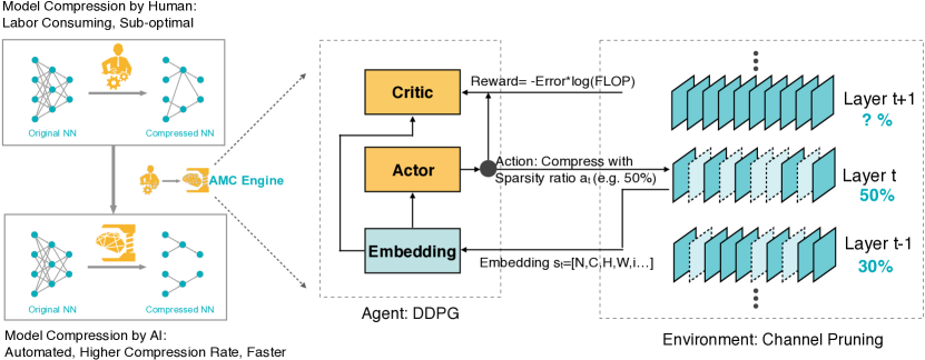
Figure 1: Overview of AutoML for Model Compression (AMC) engine. Left: AMC replaces human and makes model compression fully automated while performing better than human. Right: Form AMC as a reinforcement learning problem. We process a pre-trained network (e.g., MobileNet) in a layer-by-layer manner. Our reinforcement learning agent (DDPG) receives the embedding $s_{t}$ from a layer $t$, and outputs a sparsity ratio $a_{t}$. After the layer is compressed with $a_{t}$, it moves to the next layer $L_{t+1}$. The accuracy of the pruned model with all layers compressed is evaluated. Finally, as a function of accuracy and FLOP, reward $R$ is returned to the reinforcement learning agent.

In many machine learning applications such as robotics, self-driving cars, and advertisement ranking, deep neural networks are constrained by latency, energy and model size budget. Many approaches have been proposed to improve the hardware efficiency of neural networks by model compression [26, 19, 22]. The core of model compression technique is to determine the compression policy for each layer as they have different redundancy, which conventionally requires hand-crafted heuristics and domain expertise to explore the large design space trading off among model size, speed, and accuracy. The design space is so large that human heuristic is usually sub-optimal, and manual model compression is time-consuming. To this end, we aim to automatically find the compression policy for an arbitrary network to achieve even better performance than human designed, rule-based model compression methods.

Previously there were many rule-based model compression heuristics [20, 16]. For example, prune less parameters in the first layer which extracts low level features and have the least amount of parameters; prune more parameters in the FC layer since FC layers have the most parameters; prune less parameters in the layers that are sensitive to pruning, etc. However, as the layers in deep neural networks are not independent, these rule-based pruning policies are non-optimal, and doesn’t transfer from one model to another model. Neural network architectures are evolving fast, and we need an automated way to compress them to improve engineer efficiency. As the neural network becomes deeper, the design space has exponential complexity , which is infeasible to be solved by greedy, rule-based methods. Therefore, we propose AutoML for Model Compression (AMC) which leverages reinforcement learning to automatically sample the design space and improve the model compression quality. Figure 1 illustrates our AMC engine. When compressing a network, our AMC engine automates this process by learning-based policies, rather than relying on rule-based policy and experienced engineers.

We observe that the accuracy of the compressed model is very sensitive to the sparsity of each layer, requiring a fine-grained action space. Therefore, instead of searching over a discrete space, we come up with a continuous compression ratio control strategy with a DDPG [32] agent to learn through trial and error: penalizing accuracy loss while encouraging model shrinking and speedup. The actor-critic structure also helps to reduce variance, facilitating stabler training. Specifically, our DDPG agent processes the network in a layer-wise manner. For each layer $L_{t}$, the agent receives a layer embedding $s_{t}$ which encodes useful characteristics of this layer, and then it outputs a precise compression ratio $a_{t}$. After layer $L_{t}$ is compressed with $a_{t}$, the agent moves to the next layer $L_{t+1}$. The validation accuracy of the pruned model with all layers compressed is evaluated without fine-tuning, which is an efficient delegate of the fine-tuned accuracy. This simple approximation can improve the search time not having to retrain the model, and provide high quality search result. After the policy search is done, the best-explored model is fine-tuned to achieve the best performance.

We proposed two compression policy search protocols for different scenarios. For latency-critical AI applications (e.g., mobile apps, self-driving cars, and advertisement rankings), we propose resource-constrained compression to achieve the best accuracy given the maximum amount of hardware resources (e.g., FLOPs, latency, and model size), For quality-critical AI applications (e.g., Google Photos) where latency is not a hard constraint, we propose accuracy-guaranteed compression to achieve the smallest model with no loss of accuracy.

We achieve resource-constrained compression by constraining the search space, in which the action space (pruning ratio) is constrained such that the model compressed by the agent is always below the resources budget. For accuracy-guaranteed compression, we define a reward that is a function of both accuracy and hardware resource. With this reward function, we are able to explore the limit of compression without harming the accuracy of models.

To demonstrate the wide and general applicability, we evaluate our AMC engine on multiple neural networks, including VGG [45], ResNet [21], and MobileNet [23], and we also test the generalization ability of the compressed model from classification to object detection. Extensive experiments suggest that AMC offers better performance than hand-crafted heuristic policies. For ResNet-50, we push the expert-tuned compression ratio [16] from 3.4$\times$ to 5$\times$ with no loss of accuracy. Furthermore, we reduce the FLOPs of MobileNet [23] by 2$\times$, achieving top one accuracy of 70.2%, which is on a better Pareto curve than 0.75 MobileNet, and we achieve a speedup of 1.53$\times$ on the Titan XP and 1.95$\times$ on an Android phone.

Table 1: Comparisons of reinforcement learning approaches for models searching (NAS: Neural Architecture Search [57], NT: Network Transformation [6], N2N: Network to Network [2], and AMC: AutoML for Model Compression. AMC distinguishes from other works by getting reward without fine-tuning, continuous search space control, and can produce both accuracy-guaranteed and hardware resource-constrained models.

	NAS	NT	N2N	AMC
optimize for accuracy	✓	✓	✓	✓
optimize for latency				✓
simple, non-RNN controller				✓
fast exploration with few GPUs		✓	✓	✓
continuous action space				✓

2 Related Work

CNN Compression and Acceleration. Extensive works [20, 19, 34, 12, 18, 17] have been done on accelerating neural networks by compression. Quantization [55, 10, 41] and special convolution implementations [36, 48, 29, 3] can also speed up the neural networks. Tensor factorization [30, 15, 27, 35] decomposes weights into light-weight pieces, for example [51, 11, 14] proposed to accelerate the fully connected layers with truncated SVD; Jaderberg et al. [26] proposed to factorize layers into 1$\times$3 and 3$\times$1; and Zhang et al. [53] proposed to factorize layers into 3$\times$3 and 1$\times$1. Channel pruning [40, 24, 1, 38] removes the redundant channels from feature maps. A common problem of these methods is how to determine the sparsity ratio for each layer.

Neural Architecture Search and AutoML. Many works on searching models with reinforcement learning and genetic algorithms [46, 42, 5, 37] greatly improve the performance of neural networks. NAS [57] aims to search the transferable network blocks, and its performance surpasses many manually designed architectures [47, 21, 9]. Cai et al. [6] proposed to speed up the exploration via network transformation [8]. Inspired by them, N2N [2] integrated reinforcement learning into channel selection. In Table 1, we demonstrate several merits of our AMC engine. Compared with previous work, AMC engine optimizes for both accuracy and latency, requires a simple non-RNN controller, can do fast exploration with fewer GPU hours, and also support continuous action space.

3 Methodology

We present an overview of our AutoML for Model Compression(AMC) engine in Figure 1. We aim to automatically find the redundancy for each layer, characterized by sparsity. We train an reinforcement learning agent to predict the action and give the sparsity, then perform form the pruning. We quickly evaluate the accuracy after pruning but before fine-tuning as an effective delegate of final accuracy. Then we update the agent by encouraging smaller, faster and more accurate models.

3.1 Problem Definition

Model compression is achieved by reducing the number of parameters and computation of each layer in deep neural networks. There are two categories of pruning: fine-grained pruning and structured pruning. Fine-grained pruning [19] aims to prune individual unimportant elements in weight tensors, which is able to achieve very high compression rate with no loss of accuracy. However, such algorithms result in an irregular pattern of sparsity, and it requires specialized hardware such as EIE [18] for speed up. Coarse-grained / structured pruning [31] aims to prune entire regular regions of weight tensors (e.g., channel, row, column, block, etc.). The pruned weights are regular and can be accelerated directly with off-the-shelf hardware and libraries. Here we study structured pruning that shrink the input channel of each convolutional and fully connected layer.

Our goal is to precisely find out the effective sparsity for each layer, which used to be manually determined in previous studies [38, 31, 22]. Take convolutional layer as an example. The shape of a weight tensor is $n\times c\times k\times k$, where $n,c$ are output and input channels, and $k$ is the kernel size. For fine-grained pruning, the sparsity is defined as the number of zero elements divided by the number of total elements, i.e. $\text{\#zeros}/(n\times c\times k\times h)$. For channel pruning, we shrink the weight tensor to $n\times c^{\prime}\times k\times k$ (where $c^{\prime}<c$), hence the sparsity becomes $c^{\prime}/c$.

3.2 Automated Compression with Reinforcement Learning

AMC leverages reinforcement learning for efficient search over action space. Here we introduce the detailed setting of reinforcement learning framework.

3.2.1 The State Space

For each layer $t$, we have 11 features that characterize the state $s_{t}$:

$$(t,n,c,h,w,stride,k,FLOPs[t],reduced,rest,\textit{a}_{t-1})$$ (1)

where $t$ is the layer index, the dimension of the kernel is $n\times c\times k\times k$, and the input is $c\times h\times w$. $FLOPs[t]$ is the FLOPs of layer $L_{t}$. $Reduced$ is the total number of reduced FLOPs in previous layers. $Rest$ is the number of remaining FLOPs in the following layers. Before being passed to the agent, they are scaled within $[0,1]$. Such features are essential for the agent to distinguish one convolutional layer from another.

3.2.2 The Action Space

Most of the existing works use discrete space as coarse-grained action space (e.g., $\{64,128,256,512\}$ for the number of channels). Coarse-grained action space might not be a problem for a high-accuracy model architecture search. However, we observed that model compression is very sensitive to sparsity ratio and requires fine-grained action space, leading to an explosion of the number of discrete actions (Sec. 4.2.2). Such large action spaces are difficult to explore efficiently [32]. Discretization also throws away the order: for example, 10% sparsity is more aggressive than 20% and far more aggressive than 30%.

As a result, we propose to use continuous action space $\textit{a}\in(0,1]$, which enables more fine-grained and accurate compression.

3.2.3 DDPG Agent

As illustrated in Figure 1, the agent receives an embedding state $s_{t}$ of layer $L_{t}$ from the environment and then outputs a sparsity ratio as action $\textit{a}_{t}$. The underlying layer is compressed with $\textit{a}_{t}$ (rounded to the nearest feasible fraction) using a specified compression algorithm (e.g., channel pruning). Then the agent moves to the next layer $L_{t+1}$, and receives state $s_{t+1}$. After finishing the final layer $L_{T}$, the reward accuracy is evaluated on the validation set and returned to the agent. For fast exploration, we evaluate the reward accuracy without fine-tuning, which is a good approximation for fine-tuned accuracy (Sec. 4.1.3).

We use the deep deterministic policy gradient (DDPG) for continuous control of the compression ratio, which is an off-policy actor-critic algorithm. For the exploration noise process, we use truncated normal distribution:

$$\mu^{\prime}(s_{t})\sim\text{TN}\left(\mu\left(s_{t}\mid\theta_{t}^{\mu}\right),\sigma^{2},0,1\right)$$ (2)

During exploitation, noise $\sigma$ is initialized as $0.5$ and is decayed after each episode exponentially.

Following Block-QNN [54], which applies a variant form of Bellman’s Equation [50], each transition in an episode is $(s_{t},a_{t},R,s_{t+1})$, where $R$ is the reward after the network is compressed. During the update, the baseline reward $b$ is subtracted to reduce the variance of gradient estimation, which is an exponential moving average of the previous rewards [56, 6]:

$$\begin{gathered}Loss=\frac{1}{N}\sum_{i}\left(y_{i}-Q\left(s_{i},a_{i}\mid\theta^{Q}\right)\right)^{2}\\ y_{i}=r_{i}-b+\gamma Q(s_{i+1},\mu(s_{i+1})\mid\theta^{Q})\end{gathered}$$ (3)

The discount factor $\gamma$ is set to 1 to avoid over-prioritizing short-term rewards [4].

3.3 Search Protocols

3.3.1 Resource-Constrained Compression

By limiting the action space (the sparsity ratio for each layer), we can accurately arrive at the target compression ratio. Following [57, 4, 54], we use the following reward:

$$R_{err}=-Error$$ (4)

This reward offers no incentive for model size reduction, so we the achieve target compression ratio by an alternative way: limiting the action space. Take fine-grained pruning for model size reduction as an example: we allow arbitrary action a at the first few layers; we start to limit the action a when we find that the budget is insufficient even after compressing all the following layers with most aggressive strategy. Algorithm 1 illustrates the process. (For channel pruning, the code will be longer but similar, since removing input channels of layer $L_{t}$ will also remove the corresponding output channels of $L_{t-1}$, reducing parameters/FLOPs of both layers). Note again that our algorithm is not limited to constraining model size and it can be replaced by other resources, such as FLOPs or the actual inference time on mobile device. Based on our experiments (Sec. 4.1.1), as the agent receives no incentive for going below the budget, it can precisely arrive at the target compression ratio.

Algorithm 1 Predict the sparsity ratio $\texttt{action}_{t}$ for layer $L_{t}$ with constrained model size (number of parameters) using fine-grained pruning

$\triangleright$ Initialize the reduced model size so far

if $t$ is equal to $0$ then

     $\texttt{W}_{\text{reduced}}\leftarrow 0$

end if

$\triangleright$ Compute the agent’s action and bound it with the maximum sparsity ratio

$\texttt{action}_{t}\leftarrow\mu^{\prime}(s_{t})$

$\texttt{action}_{t}\leftarrow\min(\texttt{action}_{t},\texttt{action}_{\text{max}})$

$\triangleright$ Compute the model size of the whole model and all the later layers

$\texttt{W}_{\text{all}}\leftarrow\sum_{k}\texttt{W}_{k}$

$\texttt{W}_{\text{rest}}\leftarrow\sum_{k=t+1}\texttt{W}_{k}$

$\triangleright$ Compute the number of parameters we have to reduce in the current layer if all the later layers are pruned with the maximum sparsity ratio. $\alpha$ is the target sparsity ratio of the whole model.

$\texttt{W}_{\text{duty}}\leftarrow\alpha\cdot\texttt{W}_{\text{all}}-\texttt{action}_{\text{max}}\cdot\texttt{W}_{\text{rest}}-\texttt{W}_{\text{reduced}}$

$\triangleright$ Bound $\texttt{action}_{t}$ if it is too small to meet the target model size reduction

$\texttt{action}_{t}\leftarrow\max(\texttt{action}_{t},\texttt{W}_{\text{duty}}/\texttt{W}_{t})$

$\triangleright$ Update the accumulation of reduced model size

$\texttt{W}_{\text{reduced}}\leftarrow\texttt{W}_{\text{reduced}}+\texttt{action}_{t}\cdot\texttt{W}_{t}$

return $\texttt{action}_{t}$

3.3.2 Accuracy-Guaranteed Compression

By tweaking the reward function, we can accurately find out the limit of compression that offers no loss of accuracy. We empirically observe that $Error$ is inversely-proportional to $\log(FLOPs)$ or $\log(\#Param)$ [7]. Driven by this, we devise the following reward function:

$$R_{\text{FLOPs}}=-Error\cdot\log(\text{FLOPs})$$ (5)

$$R_{\text{Param}}=-Error\cdot\log(\text{\#Param})$$ (6)

This reward function is sensitive to $Error$; in the meantime, it provides a small incentive for reducing FLOPs or model size. Based on our experiments in Figure 4.1.2, we note that our agent automatically finds the limit of compression.

4 Experimental Results

For fine-grained pruning [19], we prune the weights with least magnitude. The maximum sparsity ratio $a_{max}$ for convolutional layers is set to 0.8, and $a_{max}$ for fully connected layer is set to 0.98. For channel pruning, we use max response selection (pruning the weights according to the magnitude [20]), and preserve Batch Normalization [25] layers during pruning instead of merging them into convolutional layers. The maximum sparsity ratios $a_{max}$ for all layers are set to 0.8. Note that the manual upper bound $a_{max}$ is only intended for faster search, one can simply use $a_{max}=1$ which also produces similar results. Our actor network $\mu$ has two hidden layers, each with 300 units. The final output layer is a sigmoid layer to bound the actions within $(0,1)$. Our critic network $Q$ also had two hidden layers, both with 300 units. Actions arr included in the second hidden layer. We use $\tau=0.01$ for the soft target updates and train the network with 64 as batch size and 2000 as replay buffer size. Our agent first explores 100 episodes with a constant noise $\sigma=0.5$, and then exploits 300 episodes with exponentially decayed noise $\sigma$.

4.1 CIFAR-10 and Analysis

We conduct extensive experiments and fully analyze our AMC on CIFAR-10 [28]to verify the effectiveness of the 2 search protocols. CIFAR dataset consists of 50k training and 10k testing $32\times 32$ tiny images in ten classes. We split the training images into 45k/5k train/validation. The accuracy reward is obtained on validation images. Our approach is computationally efficient: the RL can finish searching within 1 hour on a single GeForce GTX TITAN Xp GPU.

Table 2: Pruning policy comparison of Plain-20, ResNets [21] on CIFAR-10 [28]. $R_{\text{Err}}$ corresponds to FLOPs-constrained compression with channel pruning, while $R_{\text{Param}}$ corresponds to accuracy guaranteed compression with fine-grained pruning. For both shallow network Plain-20 and deeper network ResNets, AMC outperforms hand-crafted policies by a large margin. This enables efficient exploration without fine-tuning. Although AMC makes many trials on model architecture, we have separate validation and test dataset. No over-fitting is observed.

Model	Policy	Ratio	Val Acc.	Test Acc.	Acc. after FT.
Plain-20 (90.5%)	deep (handcraft)	50% FLOPs	79.6	79.2	88.3
	shallow (handcraft)		83.2	82.9	89.2
	uniform (handcraft)		84.0	83.9	89.7
	AMC ($R_{\text{Err}})$		86.4	86.0	90.2
ResNet-56 (92.8%)	uniform (handcraft)	50% FLOPs	87.5	87.4	89.8
	deep (handcraft)		88.4	88.4	91.5
	AMC ($R_{\text{Err}})$		90.2	90.1	91.9
ResNet-50 (93.53%)	AMC ($R_{\text{Param}})$	60% Params	93.64	93.55	-

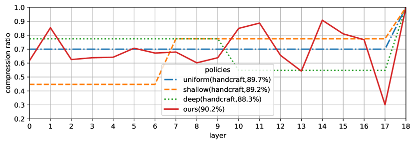
Figure 2: Comparisons of pruning strategies for Plain-20 under $2\times$. Uniform policy sets the same compression ratio for each layer uniformly. Shallow and deep policies aggressively prune shallow and deep layers respectively. Policy given by AMC looks like sawtooth, which resembles the bottleneck architecture [21]. The accuracy given by AMC outperforms hand-crafted policies. (better viewed in color)

4.1.1 FLOPs-Constrained Compression.

We conducted FLOPs-constrained experiments on CIFAR-10 with channel pruning. We compare our approach with three empirical policies [31, 22] illustrated in Figure 2: uniform sets compression ratio uniformly, shallow and deep aggressively prune shallow and deep layers respectively. Based on sparsity distribution of different networks, a different strategy might be chosen.

In Table 2, we show us using reward $R_{err}$ to accurately find the sparsity ratios for pruning 50% for Plain-20 and ResNet-56 [21] and compare it with empirical policies. We outperform empirical policies by a large margin. The best pruning setting found by AMC differs from hand-crafted heuristic (Figure 2). It learns a bottleneck architecture [21].

4.1.2 Accuracy-Guaranteed Compression.

By using the $R_{\text{Param}}$ reward, our agent can automatically find the limit of compression, with smallest model size and little loss of performance. As shown in Table 2, we compress ResNet-50 with fine-grained pruning on CIFAR-10. The result we obtain has up to 60% compression ratio with even a little higher accuracy on both validation set and test set, which might be in light of the regularization effect of pruning.

Since our reward $R_{\text{Param}}$ focuses on $Error$ and offers very little incentive to compression in the meantime, it prefers the high-performance model with harmless compression. To shorten the search time, we obtain the reward using validation accuracy without fine-tuning. We believe if reward were fine-tuned accuracy, the agent should compress more aggressively, because the fine-tuned accuracy is much closer to the original accuracy.

4.1.3 Speedup policy exploration.

Fine-tuning a pruned model usually takes a very long time. We observe a correlation between the pre-fine-tune accuracy and the post fine-tuning accuracy [20, 22]. As shown in Table 2, policies that obtain higher validation accuracy correspondingly have higher fine-tuned accuracy. This enables us to predict final model accuracy without fine-tuning, which results in an efficient and faster policy exploration.

The validation set and test set are separated, and we only use the validation set to generate reward during reinforcement learning. In addition, the compressed models have fewer parameters. As shown in Table 2, the test accuracy and validation accuracy are very close, indicating no over-fitting.

4.2 ImageNet

On ImageNet, we use 3000 images from the training set to evaluate the reward function in order to prevent over-fitting. The latency is measured with $224\times 224$ input throughout the experiments.

4.2.1 Push the Limit of Fine-grained Pruning.

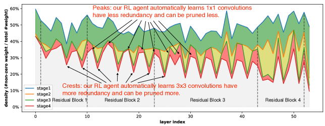
Figure 3: The pruning policy (sparsity ratio) given by our reinforcement learning agent for ResNet-50. With 4 stages of iterative pruning, we find very salient sparsity pattern across layers: peaks are $1\times 1$ convolution, crests are $3\times 3$ convolution. The reinforcement learning agent automatically learns that $3\times 3$ convolution has more redundancy than $1\times 1$ convolution and can be pruned more.

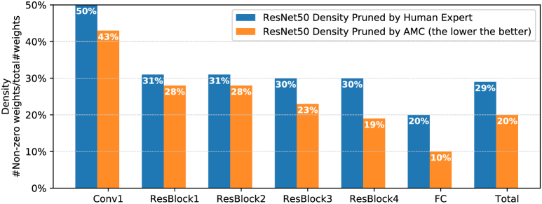
Figure 4: Our reinforcement learning agent (AMC) can prune the model to a lower density compared with human experts without losing accuracy. (Human expert: $3.4\times$ compression on ResNet50. AMC : $5\times$ compression on ResNet50.)

Fine-grained pruning method prunes neural networks based on individual connections to achieve sparsity in both weights and activations, which is able to achieve higher compression ratio and can be accelerated with specialized hardware such as [18, 17, 39]. However, it requires iterative prune & fine-tune procedure to achieve decent performance [20], and single-shot pruning without retraining will greatly hurt the prediction accuracy with large compression rate (say $4\times$), which cannot provide useful supervision for reinforcement learning agent.

To tackle the problem, we follow the settings in [16] to conduct 4-iteration pruning & fine-tuning experiments, where the overall density of the full model is set to [50%, 35%, 25% and 20%] in each iteration. For each stage, we run AMC to determine the sparsity ratio of each layer given the overall sparsity. The model is then pruned and fine-tuned for 30 epochs following common protocol. With that framework, we are able to push the expert-tuned compression ratio of ResNet-50 on ImageNet from $3.4\times$ to $\mathbf{5\times}$ (see Figure 4) without loss of performance on ImageNet (original ResNet50’s [top-1, top-5] accuracy=[76.13%, 92.86%]; AMC pruned model’s accuracy=[76.11%, 92.89%]). The density of each layer during each stage is displayed in Figure 3. The peaks and crests show that the RL agent automatically learns to prune $3\times 3$ convolutional layers with larger sparsity, since they generally have larger redundancy; while prunes more compact $1\times 1$ convolutions with lower sparsity. The density statistics of each block is provided in Figure 4. We can find that the density distribution of AMC is quite different from human expert’s result shown in Table 3.8 of [16], suggesting that AMC can fully explore the design space and allocate sparsity in a better way.

4.2.2 Comparison with Heuristic Channel Reduction.

Table 3: Learning-based model compression (AMC) outperforms rule-based model compression. Rule-based heuristics are suboptimal. (for reference, the baseline top-1 accuracy of VGG-16 is 70.5%, MobileNet is 70.6%, MobileNet-V2 is 71.8%).

	policy	FLOPs	$\Delta Acc~{}\%$
VGG-16	FP (handcraft) [31]	20%	-14.6
	RNP (handcraft) [33]		-3.58
	SPP (handcraft) [49]		-2.3
	CP (handcraft) [22]		-1.7
	AMC (ours)		-1.4
MobileNet	uniform (0.75-224) [23]	56%	-2.5
	AMC (ours)	50%	-0.4
	uniform (0.75-192) [23]	41%	-3.7
	AMC (ours)	40%	-1.7
MobileNet-V2	uniform (0.75-224) [44]	70%	-2.0
	AMC (ours)		-1.0

Here we compare AMC with existing state-of-the-art channel reduction methods: FP [31], RNP [33] and SPP [49]. All the methods proposed a heuristic strategy to design the pruning ratio of each layer. FP [31] proposed a sensitive analysis scheme to estimate the sensitivity of each layer by evaluating the accuracy with single layer pruned. Layers with lower sensitivity are pruned more aggressively. Such method assumes that errors of different pruned layers can be summed up linearly, which does not stand according to our experiments. RNP [33] groups all convolutional channels into 4 sets and trains a RL agent to decide on the 4 sets according to input image. However, the action space is very rough (only 4 actions for each layer), and it cannot reduce the model size. SPP [49] applies PCA analysis to each layer and takes the reconstruction error as the sensitivity measure to determine the pruning ratios. Such analysis is conducted based on one single layer, failing to take the correlations between layers into consideration. We also compare our method to the original channel pruning paper (CP in Table 3), in which the sparsity ratios of pruned VGG-16 [45] are carefully tuned by human experts (conv5 are skipped, sparsity ratio for conv4 and remaining layers is $1:1.5$). The results of pruned VGG-16 are presented in Table 3. Consistent with our CIFAR-10 experiments (Sec. 4.1.1), AMC outperforms all heuristic methods by more than 0.9%, and beats human expert by 0.3% without any human labor.

Apart from VGG-16, we also test AMC on modern efficient neural networks MobileNet [23] and MobileNet-V2 [44]. Since the networks have already been very compact, it is much harder to further compress them. The easiest way to reduce the channels of a model is to use uniform channel shrinkage, i.e. use a width multiplier to uniformly reduce the channels of each layer with a fixed ratio. Both MobileNet and MobileNet-V2 present the performance of different multiplier and input sizes, and we compare our pruned result with models of same computations. The format are denoted as uniform (depth multiplier - input size). We can find that our method consistently outperforms the uniform baselines. Even for the current state-of-the-art efficient model design MobileNet-V2, AMC can still improve its accuracy by $1.0\%$ at the same computation (Table 3). The pareto curve of MobileNet is presented in Figure 5(a).

4.2.3 Speedup Mobile Inference.

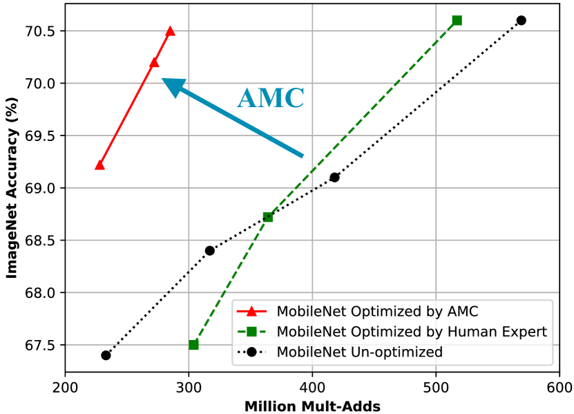
(a) Accuracy v.s. MACs

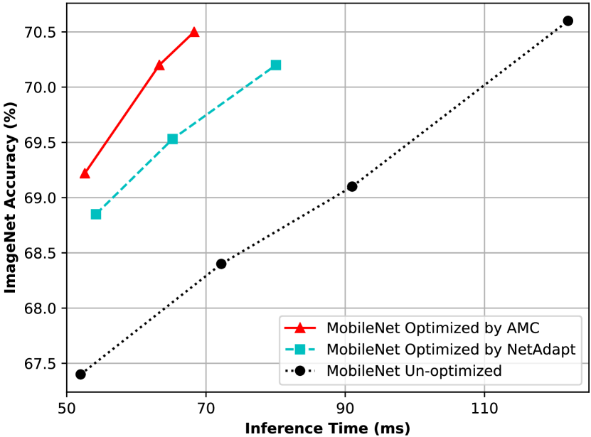
(b) Accuracy v.s. Inference time

Figure 5: (a) Comparing the accuracy and MAC trade-off among AMC, human expert, and unpruned MobileNet. AMC strictly dominates human expert in the pareto optimal curve. (b) Comparing the accuracy and latency trade-off among AMC, NetAdapt, and unpruned MobileNet. AMC significantly improves the pareto curve of MobileNet. Reinforcement-learning based AMC surpasses heuristic-based NetAdapt on the pareto curve (inference time both measured on Google Pixel 1).

Table 4: AMC speeds up MobileNet. Previous attempts using rule-based policy to prune MobileNet lead to significant accuracy degradation [31] while AMC use learning-based pruning which well preserve the accuracy. On Google Pixel-1 CPU, AMC achieves $1.95\times$ measured speedup with batch size one, while saving the memory by 34%. On NVIDIA Titan XP GPU, AMC achieves $1.53\times$ speedup with batch size of 50. The input image size is 224$\times$224 for all experiments and no quantization is applied for apple-to-apple comparison.

	Million MAC	top-1 acc.	top-5 acc.	GPU		Android
				latency	speed	latency	speed	memory
100% MobileNet	569	70.6%	89.5%	0.46ms	2191 fps	123.3ms	8.1 fps	20.1MB
75% MobileNet	325	68.4%	88.2%	0.34ms	2944 fps	72.3ms	13.8 fps	14.8MB
NetAdapt [52]	-	69.8%	-	-	-	70.0ms	14.3 fps	-
AMC ($50\%$ FLOPs)	285	70.5%	89.3%	0.32ms	3127 fps (1.43$\times$)	68.3ms	14.6 fps (1.81$\times$)	14.3MB
AMC ($50\%$ Latency)	272	70.2%	89.2%	0.30ms	3350 fps (1.53$\times$)	63.3ms	16.0 fps (1.95$\times$)	13.2MB

Mobile inference acceleration has drawn people’s attention in recent years. Not only can AMC optimize FLOPs and model size, it can also optimize the inference latency, directly benefiting mobile developers. For all mobile inference experiments, we use TensorFlow Lite framework for timing evaluation.

We prune MobileNet [23], a highly compact network consisting of depth-wise convolution and point-wise convolution layers, and measure how much we can improve its inference speed. Previous attempts using hand-crafted policy to prune MobileNet led to significant accuracy degradation [31]: pruning MobileNet to 75.5% original parameters results in 67.2% top-1 accuracy, which is even worse than the original 0.75 MobileNet (61.9% parameters with 68.4% top-1 accuracy). However, our AMC pruning policy significantly improves pruning quality: on ImageNet, AMC-pruned MobileNet achieved 70.5% Top-1 accuracy with 285 MFLOPs, compared to the original 0.75 MobileNet’s 68.4% Top-1 accuracy with 325 MFLOPs. As illustrated in Figure 5(a), human expert’s hand-crafted policy achieves slightly worse performance than that of the original MobileNet under $2\times$ FLOPs reduction. However, with AMC, we significantly raise the pareto curve, improving the accuracy-MACs trade-off of original MobileNet.

By substituting FLOPs with latency, we can change from FLOPs-constrained search to latency-constrained search and directly optimize the inference time. Our experiment platform is Google Pixel 1 with Qualcomm Snapdragon 821 SoC. As shown in Figure 5(b), we greatly reduce the inference time of MobileNet under the same accuracy. We also compare our learning based policy with a heuristic-based policy [52], and AMC better trades off accuracy and latency. Furthermore, since AMC uses the validation accuracy before fine-tuning as the reward signal while [52] needs local fine-tuning after each step, AMC is more sampling-efficient, requiring fewer GPU hours for policy search.

We show the detailed statistics of our pruned model in Table 4. Model searched with 0.5$\times$ FLOPs and 0.5$\times$ inference time are profiled and displayed. For 0.5$\times$ FLOPs setting, we achieve 1.81$\times$ speed up on a Google Pixel 1 phone, and for 0.5$\times$ FLOPs setting, we accurately achieve 1.95$\times$ speed up, which is very close to actual 2$\times$ target, showing that AMC can directly optimize inference time and achieve accurate speed up ratio. We achieve 2.01$\times$ speed up for 1$\times$1 convolution but less significant speed up for depth-wise convolution due to the small computation to communication ratio. AMC compressed models also consumes less memory. On GPUs, we also achieve up to 1.5$\times$ speedup, less than mobile phone, which is because a GPU has higher degree of parallelism than a mobile phone.

4.2.4 Generalization Ability.

Table 5: Compressing Faster R-CNN with VGG16 on PASCAL VOC 2007. Consistent with classification task, AMC also results in better performance under the same compression ratio on object detection task.

	mAP (%)	mAP [0.5, 0.95] (%)
baseline	68.7	36.7
$2\times$ handcrafted [22]	68.3 (-0.4)	36.7 (-0.0)
$4\times$ handcrafted [22]	66.9 (-1.8)	35.1 (-1.6)
$4\times$ handcrafted [53]	67.8 (-0.9)	36.5 (-0.2)
$4\times$ AMC (ours)	68.8 (+0.1)	37.2 (+0.5)

We evaluate the generalization ability of AMC on PASCAL VOC object detection task [13]. We use the compressed VGG-16 (from Sec 4.2.2) as the backbone for Faster R-CNN [43]. In Table 5, AMC achieves 0.7% better mAP[0.5, 0.95]) than the best hand-crafted pruning methods under the same compression ratio. AMC even surpasses the baseline by 0.5% mAP. We hypothesize this improvement as that the optimal compression policy found by the RL agent also serves as effective regularization.

5 Conclusion

Conventional model compression techniques use hand-crafted features and require domain experts to explore a large design space and trade off between model size, speed, and accuracy, which is usually suboptimal and labor-consuming. In this paper, we propose AutoML for Model Compression (AMC), which leverages reinforcement learning to automatically search the design space, greatly improving the model compression quality. We also design two novel reward schemes to perform both resource-constrained compression and accuracy-guaranteed compression. Compelling results have been demonstrated for MobileNet, MobileNet-V2, ResNet and VGG on Cifar and ImageNet. The compressed model generalizes well from classification to detection tasks. On the Google Pixel 1 mobile phone, we push the inference speed of MobileNet from 8.1 fps to 16.0 fps. AMC facilitates efficient deep neural networks design on mobile devices.

References

- [1] Anwar, S., Sung, W.: Compact deep convolutional neural networks with coarse pruning. arXiv preprint arXiv:1610.09639 (2016)
- [2] Ashok, A., Rhinehart, N., Beainy, F., Kitani, K.M.: N2n learning: Network to network compression via policy gradient reinforcement learning. arXiv preprint arXiv:1709.06030 (2017)
- [3] Bagherinezhad, H., Rastegari, M., Farhadi, A.: Lcnn: Lookup-based convolutional neural network. arXiv preprint arXiv:1611.06473 (2016)
- [4] Baker, B., Gupta, O., Naik, N., Raskar, R.: Designing neural network architectures using reinforcement learning. arXiv preprint arXiv:1611.02167 (2016)
- [5] Brock, A., Lim, T., Ritchie, J.M., Weston, N.: Smash: one-shot model architecture search through hypernetworks. arXiv preprint arXiv:1708.05344 (2017)
- [6] Cai, H., Chen, T., Zhang, W., Yu, Y., Wang, J.: Reinforcement learning for architecture search by network transformation. arXiv preprint arXiv:1707.04873 (2017)
- [7] Canziani, A., Paszke, A., Culurciello, E.: An analysis of deep neural network models for practical applications. arXiv preprint arXiv:1605.07678 (2016)
- [8] Chen, T., Goodfellow, I., Shlens, J.: Net2net: Accelerating learning via knowledge transfer. arXiv preprint arXiv:1511.05641 (2015)
- [9] Chollet, F.: Xception: Deep learning with depthwise separable convolutions. arXiv preprint arXiv:1610.02357 (2016)
- [10] Courbariaux, M., Bengio, Y.: Binarynet: Training deep neural networks with weights and activations constrained to+ 1 or-1. arXiv preprint arXiv:1602.02830 (2016)
- [11] Denton, E.L., Zaremba, W., Bruna, J., LeCun, Y., Fergus, R.: Exploiting linear structure within convolutional networks for efficient evaluation. In: Advances in Neural Information Processing Systems. pp. 1269–1277 (2014)
- [12] Dong, X., Huang, J., Yang, Y., Yan, S.: More is less: A more complicated network with less inference complexity. arXiv preprint arXiv:1703.08651 (2017)
- [13] Everingham, M., Van Gool, L., Williams, C.K.I., Winn, J., Zisserman, A.: The PASCAL Visual Object Classes Challenge 2007 (VOC2007) Results. http://www.pascal-network.org/challenges/VOC/voc2007/workshop/index.html
- [14] Girshick, R.: Fast r-cnn. In: Proceedings of the IEEE International Conference on Computer Vision. pp. 1440–1448 (2015)
- [15] Gong, Y., Liu, L., Yang, M., Bourdev, L.: Compressing deep convolutional networks using vector quantization. arXiv preprint arXiv:1412.6115 (2014)
- [16] Han, S.: Efficient methods and hardware for deep learning, https://stacks.stanford.edu/file/druid:qf934gh3708/EFFICIENT%20METHODS%20AND%20HARDWARE%20FOR%20DEEP%20LEARNING-augmented.pdf
- [17] Han, S., Kang, J., Mao, H., Hu, Y., Li, X., Li, Y., Xie, D., Luo, H., Yao, S., Wang, Y., et al.: Ese: Efficient speech recognition engine with sparse lstm on fpga. In: Proceedings of the 2017 ACM/SIGDA International Symposium on Field-Programmable Gate Arrays. pp. 75–84. ACM (2017)
- [18] Han, S., Liu, X., Mao, H., Pu, J., Pedram, A., Horowitz, M.A., Dally, W.J.: Eie: efficient inference engine on compressed deep neural network. In: Proceedings of the 43rd International Symposium on Computer Architecture. pp. 243–254. IEEE Press (2016)
- [19] Han, S., Mao, H., Dally, W.J.: Deep compression: Compressing deep neural networks with pruning, trained quantization and huffman coding. arXiv preprint arXiv:1510.00149 (2015)
- [20] Han, S., Pool, J., Tran, J., Dally, W.: Learning both weights and connections for efficient neural network. In: Advances in Neural Information Processing Systems. pp. 1135–1143 (2015)
- [21] He, K., Zhang, X., Ren, S., Sun, J.: Deep residual learning for image recognition. In: Proceedings of the IEEE Conference on Computer Vision and Pattern Recognition. pp. 770–778 (2016)
- [22] He, Y., Zhang, X., Sun, J.: Channel pruning for accelerating very deep neural networks. In: Proceedings of the IEEE Conference on Computer Vision and Pattern Recognition. pp. 1389–1397 (2017)
- [23] Howard, A.G., Zhu, M., Chen, B., Kalenichenko, D., Wang, W., Weyand, T., Andreetto, M., Adam, H.: Mobilenets: Efficient convolutional neural networks for mobile vision applications. arXiv preprint arXiv:1704.04861 (2017)
- [24] Hu, H., Peng, R., Tai, Y.W., Tang, C.K.: Network trimming: A data-driven neuron pruning approach towards efficient deep architectures. arXiv preprint arXiv:1607.03250 (2016)
- [25] Ioffe, S., Szegedy, C.: Batch normalization: Accelerating deep network training by reducing internal covariate shift. arXiv preprint arXiv:1502.03167 (2015)
- [26] Jaderberg, M., Vedaldi, A., Zisserman, A.: Speeding up convolutional neural networks with low rank expansions. arXiv preprint arXiv:1405.3866 (2014)
- [27] Kim, Y.D., Park, E., Yoo, S., Choi, T., Yang, L., Shin, D.: Compression of deep convolutional neural networks for fast and low power mobile applications. arXiv preprint arXiv:1511.06530 (2015)
- [28] Krizhevsky, A., Hinton, G.: Learning multiple layers of features from tiny images (2009)
- [29] Lavin, A.: Fast algorithms for convolutional neural networks. arXiv preprint arXiv:1509.09308 (2015)
- [30] Lebedev, V., Ganin, Y., Rakhuba, M., Oseledets, I., Lempitsky, V.: Speeding-up convolutional neural networks using fine-tuned cp-decomposition. arXiv preprint arXiv:1412.6553 (2014)
- [31] Li, H., Kadav, A., Durdanovic, I., Samet, H., Graf, H.P.: Pruning filters for efficient convnets. arXiv preprint arXiv:1608.08710 (2016)
- [32] Lillicrap, T.P., Hunt, J.J., Pritzel, A., Heess, N., Erez, T., Tassa, Y., Silver, D., Wierstra, D.: Continuous control with deep reinforcement learning. arXiv preprint arXiv:1509.02971 (2015)
- [33] Lin, J., Rao, Y., Lu, J.: Runtime neural pruning. In: Advances in Neural Information Processing Systems. pp. 2178–2188 (2017)
- [34] Luo, J.H., Wu, J., Lin, W.: Thinet: A filter level pruning method for deep neural network compression. arXiv preprint arXiv:1707.06342 (2017)
- [35] Masana, M., van de Weijer, J., Herranz, L., Bagdanov, A.D., Alvarez, J.M.: Domain-adaptive deep network compression. In: The IEEE International Conference on Computer Vision (ICCV) (Oct 2017)
- [36] Mathieu, M., Henaff, M., LeCun, Y.: Fast training of convolutional networks through ffts. arXiv preprint arXiv:1312.5851 (2013)
- [37] Miikkulainen, R., Liang, J., Meyerson, E., Rawal, A., Fink, D., Francon, O., Raju, B., Navruzyan, A., Duffy, N., Hodjat, B.: Evolving deep neural networks. arXiv preprint arXiv:1703.00548 (2017)
- [38] Molchanov, P., Tyree, S., Karras, T., Aila, T., Kautz, J.: Pruning convolutional neural networks for resource efficient transfer learning. CoRR, abs/1611.06440 (2016)
- [39] Parashar, A., Rhu, M., Mukkara, A., Puglielli, A., Venkatesan, R., Khailany, B., Emer, J., Keckler, S., Dally, W.J.: Scnn: An accelerator for compressed-sparse convolutional neural networks. In: 44th International Symposium on Computer Architecture (2017)
- [40] Polyak, A., Wolf, L.: Channel-level acceleration of deep face representations. IEEE Access 3, 2163–2175 (2015)
- [41] Rastegari, M., Ordonez, V., Redmon, J., Farhadi, A.: Xnor-net: Imagenet classification using binary convolutional neural networks. In: European Conference on Computer Vision. pp. 525–542. Springer (2016)
- [42] Real, E., Moore, S., Selle, A., Saxena, S., Suematsu, Y.L., Le, Q., Kurakin, A.: Large-scale evolution of image classifiers. arXiv preprint arXiv:1703.01041 (2017)
- [43] Ren, S., He, K., Girshick, R., Sun, J.: Faster r-cnn: Towards real-time object detection with region proposal networks. In: Advances in neural information processing systems. pp. 91–99 (2015)
- [44] Sandler, M., Howard, A., Zhu, M., Zhmoginov, A., Chen, L.C.: Inverted residuals and linear bottlenecks: Mobile networks for classification, detection and segmentation. arXiv preprint arXiv:1801.04381 (2018)
- [45] Simonyan, K., Zisserman, A.: Very deep convolutional networks for large-scale image recognition. arXiv preprint arXiv:1409.1556 (2014)
- [46] Stanley, K.O., Miikkulainen, R.: Evolving neural networks through augmenting topologies. Evolutionary computation 10(2), 99–127 (2002)
- [47] Szegedy, C., Liu, W., Jia, Y., Sermanet, P., Reed, S., Anguelov, D., Erhan, D., Vanhoucke, V., Rabinovich, A.: Going deeper with convolutions. In: Proceedings of the IEEE Conference on Computer Vision and Pattern Recognition. pp. 1–9 (2015)
- [48] Vasilache, N., Johnson, J., Mathieu, M., Chintala, S., Piantino, S., LeCun, Y.: Fast convolutional nets with fbfft: A gpu performance evaluation. arXiv preprint arXiv:1412.7580 (2014)
- [49] Wang, H., Zhang, Q., Wang, Y., Hu, R.: Structured probabilistic pruning for deep convolutional neural network acceleration. arXiv preprint arXiv:1709.06994 (2017)
- [50] Watkins, C.J.C.H.: Learning from delayed rewards. Ph.D. thesis, King’s College, Cambridge (1989)
- [51] Xue, J., Li, J., Gong, Y.: Restructuring of deep neural network acoustic models with singular value decomposition. In: INTERSPEECH. pp. 2365–2369 (2013)
- [52] Yang, T.J., Howard, A., Chen, B., Zhang, X., Go, A., Sze, V., Adam, H.: Netadapt: Platform-aware neural network adaptation for mobile applications. arXiv preprint arXiv:1804.03230 (2018)
- [53] Zhang, X., Zou, J., He, K., Sun, J.: Accelerating very deep convolutional networks for classification and detection. IEEE transactions on pattern analysis and machine intelligence 38(10), 1943–1955 (2016)
- [54] Zhong, Z., Yan, J., Liu, C.L.: Practical network blocks design with q-learning. arXiv preprint arXiv:1708.05552 (2017)
- [55] Zhu, C., Han, S., Mao, H., Dally, W.J.: Trained ternary quantization. arXiv preprint arXiv:1612.01064 (2016)
- [56] Zoph, B., Le, Q.V.: Neural architecture search with reinforcement learning. arXiv preprint arXiv:1611.01578 (2016)
- [57] Zoph, B., Vasudevan, V., Shlens, J., Le, Q.V.: Learning transferable architectures for scalable image recognition. arXiv preprint arXiv:1707.07012 (2017)