Signal-background discrimination with convolutional neural networks in the PandaX-III experiment using MC simulation

Abstract

The PandaX-III experiment will search for neutrinoless double beta decay of ¹³⁶Xe with high pressure gaseous time projection chambers at the China Jin-Ping underground Laboratory. The tracking feature of gaseous detectors helps suppress the background level, resulting in the improvement of the detection sensitivity. We study a method based on the convolutional neural networks to discriminate double beta decay signals against the background from high energy gammas generated by ²¹⁴Bi and ²⁰⁸Tl decays based on detailed Monte Carlo simulation. Using the 2-dimensional projections of recorded tracks on two planes, the method successfully suppresses the background level by a factor larger than 100 with a high signal efficiency. An improvement of $62\%$ on the efficiency ratio of $\epsilon_{s}/\sqrt{\epsilon_{b}}$ is achieved in comparison with the baseline in the PandaX-III conceptual design report.

neutrino, double beta decay, convolutional neural networks, background suppression

PACS number(s): 14.60.Pq, 23.40.-s, 07.05.Mh

1 Introduction

The Dirac or Majorana nature of neutrinos is one of the most fundamental questions in particle physics. The conservation of the lepton number will be violated if neutrinos are Majorana fermions, which is intricately related to the matter-antimatter asymmetry in our universe [1]. The so-called neutrinoless double beta decay (NLDBD) process, in which a nucleus with even atomic number $Z$ and even neutron number $N$ emits two electrons simultaneously without neutrinos, is possible if neutrinos are Majorana. Therefore experimental identification of such rare process would be an important breakthrough of particle physics. ¹³⁶Xe is a widely used isotope in experiments searching for NLDBD due to its high abundance in natural xenon and relatively low cost of enrichment. Experiments using this target include KamLAND-Zen [2], EXO-200 [3], and NEXT [4].

The PandaX-III project plans to construct a ton-scale NLDBD experiment in the China Jin-Ping underground Laboratory (CJPL) using time projection chambers (TPCs) filled with high pressure xenon gas with enriched ¹³⁶Xe [5]. The first detector will have 200 kg xenon gas at 10 bar pressure and read out ionized electrons directly with Micromegas (Micro-MEsh Gaseous Structure) detectors. Trimethylamine (TMA) mixed with xenon converts part of the scintillation in xenon to ionization and improves energy resolution of the TPC. The energy resolution at ¹³⁶Xe NLDBD Q-value (2.458 MeV) is expected to reach 3% (Full-Width-Half-Maximum, FWHM). The admixture also suppresses diffusion of ionized electrons and improves the tracking capability.

The main backgrounds in the Region of Interest (ROI) of PandaX-III are high energy gamma rays from the decay of ²¹⁴Bi (2.447 MeV) and ²⁰⁸Tl (2.614 MeV) in the detector materials. These background events may fall in the same energy window of NLDBD Q-Value and mimic a signal event. The high pressure gaseous TPC is capable of recording the tracks of ionizing particles within it, providing additional information about the events besides the total energy depositions. Electrons with energy of 1 MeV travel in average 10 cm in the PandaX-III detector. At the end of an electron trajectory, the energy loss per unit length ($dE/dx$) increases dramatically, known as Bragg peak. NLDBD will have two simultaneous electron tracks in different directions and thus two distinctive Bragg peaks. This feature can be used to distinguish the NLDBD signal from gamma backgrounds. The topological signatures of ¹³⁶Xe NLDBD events and gamma rays have been studied by the NEXT collaboration [6, 7], and an extra background rejection factor is achieved by reconstructing the tracks and identifying the end point energies. It is expected that similar method could provide a background rejection factor of 35, which serves as a baseline in PandaX-III.

The topological particle identification method, like other traditional event classification methods used in particle physics, requires the reconstruction of designed expert features of the events with sophisticated algorithms for signal classification. The usage of deep neural networks in the particle physics for classification without the aid of designed features has been explored in recent years, and outstanding performance has been obtained[8, 9]. Convolutional neural networks (CNN), an artificial neural network originally developed for image analysis, have gained popularity in particle physics experiments these years [10, 11, 12, 13, 14]. CNN is especially suited for signal-background discrimination of electron tracks in the gaseous TPC. The NEXT collaboration has studied the background rejection power of CNN in the search of NLDBD by using images with all three dimensional projections of the tracks, and obtained an improvement compared with the method based on the same topological information [15]. But such a method cannot be used in the first phase of PandaX-III directly due to its strip readout. An alternative way of data preparation should be considered.

In this work, we apply the CNN technique to the signal and background discrimination in the PandaX-III experiment, based on a detailed Monte Carlo (MC) simulation with detector geometry and realistic drifting of ionized electrons. This article is organized as follows. In Sec. 2, we give a brief introduction to the PandaX-III detector and the properties of NLDBD events in it. In Sec. 3, we describe the simulation of NLDBD events in PandaX-III. Then we introduce the method of classification of NLDBD signals and backgrounds with convolutional neural networks in Sec. 4. We present the results based on Monte Carlo simulation in Sec. 4.3. A short summary is given in the last section.

2 The PandaX-III detector and background suppression

A detailed introduction to the PandaX-III detector can be found in the conceptual design report (CDR) [5]. A high pressure gaseous TPC is adopted due to its higher energy resolution in comparison with liquid detectors, and the capability of imaging the electron tracks. Deposited energy inside the TPC will be released in the form of scintillation light and ionized electrons. The electrons will drift towards the ends of the TPC due to the strong electric field and be finally collected by the readout planes. The first TPC module will be filled with 200 kg $90\%$ enriched ¹³⁶Xe with $1\%$ TMA mixture. In the second phase, the ton-scale experiment will have 5 independent detector modules, each of which will contain 200 kg of xenon gas.

The mixed gas of 10 bar pressure will be enclosed in an Oxygen-Free High Conductivity (OFHC) copper pressure vessel of cylindrical shape with a length about 2 m and diameter about 1.5 m. The total volume of the vessel is about 3.5 m³. A cylindrical TPC, with two drift regions separated by a cathode plane in the middle, will be placed inside the vessel. Each drift region will have a drift length of about 1 m and a design drift field of 1000 V/cm, shaped by the field cage. Two options to build the cylindrical field cage have been considered. The classical design with copper rings has been used widely in other experiments, including the PandaX-I [16] and PandaX-II [17] dark matter experiments. This option will be the baseline design of PandaX-III and it has been used in all our MC simulations. Another design using Diamond-Like-Carbon (DLC) coated on Kapton films may reduce difficulties during the construction and overall background rate. This approach is currently under active R&D within PandaX-III collaboration.

A special realization of Micromegas, called Microbulk, will be used in the first phase of PandaX-III to detect the ionization electrons. An excellent energy resolution of $3\%$ Full-Width-Half-Maximum (FWHM) at the NLDBD Q-value is expected based on R&D results at 10 bar of Xe with TMA by the T-REX project [18]. Each readout plane of the PandaX-III detector will be covered by 41 specially designed $20\times 20$ cm² Microbulk Micromegas (MM) modules, and each module will be read out by 128 channels of X-Y strips of 3 mm pitch (64 in each direction). The total number of readout channels is about 10000.

According to the detailed Geant4 [19, 20] based MC simulation, the main background contributions come from the high energy gamma rays generated by the radioactive descendants of ²³⁸U and ²³²Th inside the detector [5]. Steel bolts and MM modules contribute to the majority of the backgrounds within the energy window of $(Q_{\beta\beta}-2\sigma,Q_{\beta\beta}+2\sigma)$, where $\sigma$ is the corresponding standard deviation at the expected detector resolution of $3\%$. By assuming the input material activity and taking the electron diffusion and the detector response into consideration, the background index (BI) is about $3\times 10^{-3}$ counts/(keV$\cdot$kg$\cdot$year) [5]. That means that about 70 background events would be observed in the energy windows each year, which is too high for a NLDBD experiment.

Topological information of an event track, such as track length, shape, and energy deposition per unit distance, can help suppress background events further. This powerful background suppression capability has been demonstrated by other studies [18, 7]. The two high energy electrons produced in the NLDBD process will generate large amount of ionization electrons along their path inside the high pressure xenon gas and lose energy quickly, generally resulting in tracks with length of about 15 cm and higher energy depositions at the ends due to the Bragg peaks of electrons. The gamma background loses energy mostly through Compton scattering or photoelectric interactions, and the number of tracks may vary. Ideally, such topological information can be easily used if the track is fully reconstructed in 3D spaces. In the first phase of PandaX-III, the $z$ position of the energy deposition, characterizing the drifting time of electrons, can be extracted easily. But the $x$-$y$ position on the readout plane can not be determined exactly because of the ambiguity introduced by multiple strip signals at the same time. Though the 3D reconstruction is difficult, the projection of the tracks in the $x$-$z$ and $y$-$z$ will be easily acquired. It is necessary to find out a method to make use of all the information from this incomplete tracking in order to better discriminate signal and background.

3 Simulation of NLDBD events in PandaX-III

The study was carried out with MC simulation events. BambooMC, a MC program based on the Geant4 toolkit, was used to perform detailed simulation of tracking of electrons and gamma within the PandaX-III detector. The detailed structure of the detector module, including the copper vessel, the gas mixture, the field cage with copper rings and the readout planes, was constructed in the simulation(see Fig. 1). The gas mixture contains $99\%$ (mass fraction) ¹³⁶Xe enriched (at the level of $90\%$) xenon gas and $1\%$ TMA. The electric field of 1000 V/cm along the $z$ direction was also applied in the simulation.

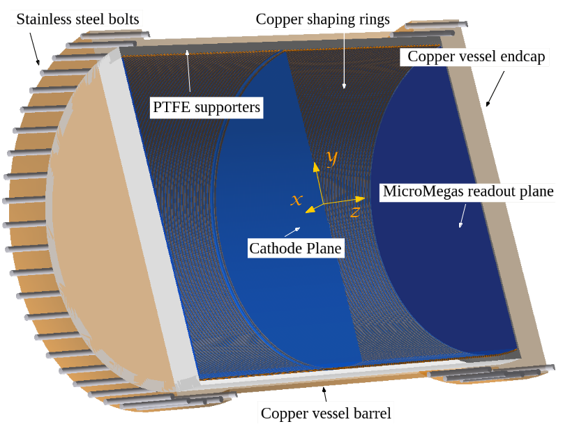
Figure 1: A cross-sectional view of the simulated PandaX-III detector.

The DECAY0 package [21] was used to generate the NLDBD signal events, each contains two electrons with a total kinetic energy around the Q-value. These events were sampled uniformly inside the gas mixture within the TPC. For the backgrounds, gamma with the energy of 2447.7 keV (from ²¹⁴Bi) and 2614 keV (from ²⁰⁸Tl) are sampled from the copper vessel volume with an isotropic angular distribution.

After the simulation, the information of particle energy depositions inside the TPC, including the position, time, energy and particle type, were recorded in the output file, serving as the input of the following digitization step. Each readout channel’s waveform, expressed by a time series of electrons arriving the corresponding area in the readout plane, was generated by simulating the generation, drifting and diffusion of the ionization electrons during the digitization.

For each energy deposition, the number of ionization electrons is randomly sampled with the W-value of 21.9 eV and Fano factor of 0.14 [22]. The drifting velocity and diffusion parameters of ionization electrons were calculated with the Magboltz [23] package through the interface of Garfield++ [24] by taking the constituent of the gas mixture and electric field into consideration. In this study, we continued to use the drifting velocity of 1.87 mm/$\mu$s, the transverse diffusion parameter of $1.02\times 10^{-2}$ cm^1/2 and the longitudinal diffusion parameter of $1.39\times 10^{-2}$ cm^1/2 [5].

For each ionization electron, the time and position when it arrives the readout plane is calculated with the initial position of the energy deposition together with the parameters. Then the possible fired readout channel is determined according to the arrangement of the MM modules and channels. The electron loss during the drifting is ignored. In real experiment, the gas will be purified continuously by the online recycling system.

We obtained a set of time series of recorded electron number for all the readout channels after iterating all the depositions in the TPC. The width of the time bin is determined assuming a sampling rate of 5 Ms/sec. An example of such a time series is shown in Fig. 2. Because the readout window is limited to 102.4 $\mu$s (512 time bins) and the maximum drifting time in one chamber of the PandaX-III TPC is about 535 $\mu$s, the waveforms may contain only part of the long time series. To simulate the trigger, We used the integrated energy, which is translated from the number of electrons, in a sliding window of 256 bins along the time axis, as a trigger. The event is “triggered” when the energy exceeds $Q_{\beta\beta}/2=1.229$ MeV. Two hundred fifty-six bins before the trigger signal and 256 bins after are rept in the final waveform. These waveforms simulate the outputs from real detector electronics. The summation of the total number of electrons are translated directly into the readout energy without additional smearing applied.

After the detailed simulation and digitization, we found the detection efficiency of NLDBD signal is 56.2$\%$ within the energy window of $Q_{\beta\beta}\pm 2\sigma$, i.e., $[2395,2520]$ keV, assuming a detector resolution of $3\%$ full width half maximum (FWHM). The value is consistent with that reported in the PandaX-III CDR.

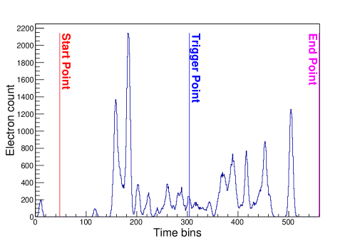
Figure 2: The number of electrons hitting a readout plane in an event by time. The bin width is 20ns. Time 0 is defined as the time when the first electron reaches the readout plane. The time series between the start point and the end point are finally recorded.

4 Event Classification with CNN

The rapid development and application of the deep neural networks, especially the usage of CNN in image classification in recent years  [25, 26], provide a possibility for the discrimination of signal and background in PandaX-III without fully reconstructing the tracks.

4.1 Introduction of CNN

A detailed introduction to the CNN can be found in Ref. [26]. We introduce the basic ideas here. Similar to the ordinary neural networks, the basic block of CNNs is neuron, which generates output value according to the input and its own parameters. Neurons are grouped into layers by their different functionalities, and the network is a stacking of the layers. Each layer of the network can be regarded as a non linear tranformation that maps a tensor(multidimensional arrays) to another tensor, so the whole network is mostly like a complicated transformation which tries to fit the input tensors to the output tensors.

CNNs are specially designed to work with image data, by reducing the parameter space with “convolution”. The first layer of a CNN reads data from images of certain size, and the last layer generates the result of classification by arranging all neurons in a row. A CNN may contain one or more convolutional layers, in which each neuron is used to compute the dot product (convolution) of its weight and values from a small region in the input volume. With such structures, CNNs are capable of learning features from given images during the training procedure so that they can be used to classify new images by recognizing their features with the same algorithm.

It was shown that significant improvement on the performance had been achieved with higher network depth [27]. But a degradation problem appears when the network becomes deeper, together with higher training error [28]. The residual network (ResNet), introduces shortcut connections between nonadjacent layers to mitigate the problem [29] and shows outstanding performance. In our study, we used the 50-layer ResNet-50 within the Keras [30] deep learning library. The input and output layers of the network have been modified so that it can accept our input data and generate an output value between 0 (exact background) and 1 (exact signal). The detailed network structure is given in Table 1.

layer name	layer type	output tensor	layer attribute	repetition
input_1	InputLayer	240, 240, 3
conv1 block	Convolution2D	120, 120, 64	7$\times$7, 64
pooling	MaxPooling2D	59, 59, 64
conv2 block	Convolution2D	59, 59, 64	1$\times$1, 64	3
	Convolution2D	59, 59, 64	3$\times$3, 64
	Convolution2D	59, 59, 256	1$\times$1, 256
conv3 block	Convolution2D	30, 30, 128	1$\times$1, 128	4
	Convolution2D	30, 30, 128	3$\times$3, 128
	Convolution2D	30, 30, 512	1$\times$1, 512
conv4 block	Convolution2D	15, 15, 256	1$\times$1, 256	6
	Convolution2D	15, 15, 256	3$\times$3, 256
	Convolution2D	15, 15, 1024	1$\times$1, 1024
conv5 block	Convolution2D	8, 8, 512	1$\times$1, 512	3
	Convolution2D	8, 8, 512	3$\times$3, 512
	Convolution2D	8, 8, 2048	1$\times$1, 2048
pooling	AveragePooling2D	1, 1, 2048
flatten	Flatten	2048
dense	Dense	256	relu
dropout	Dropout	256
dense	Dense	1	sigmoid

Table 1: The structure of the modified ResNet-50. The “repetition” column indicates the number of times the block appears in the network, and the default value is 1.

4.2 Preparation of Input Data

Since CNNs need images as the input, the MC events after digitization need to be converted to images. We converted each event to an image of $60\times 60$ pixels with the PNG format. For each readout signal by the vertically/horizontally arranged strips, its coordinate of $(x,z)$/$(y,z)$ was mapped to the image coordinates $(X,Y)$, and corresponding energy was encoded in the red/green color channel. In this way the two projections were merged into one picture. The center of the image was chosen to be the energy-weighted center of the hits to ensure most of the energy of the event could be encoded in the image. Each pixel in an image represents an area of $3\times 3$ mm² in the $xz$ and $yz$ planes of the corresponding event, so the total area is $180\times 180$ mm². An example of such a mapping is shown in Fig. 3.

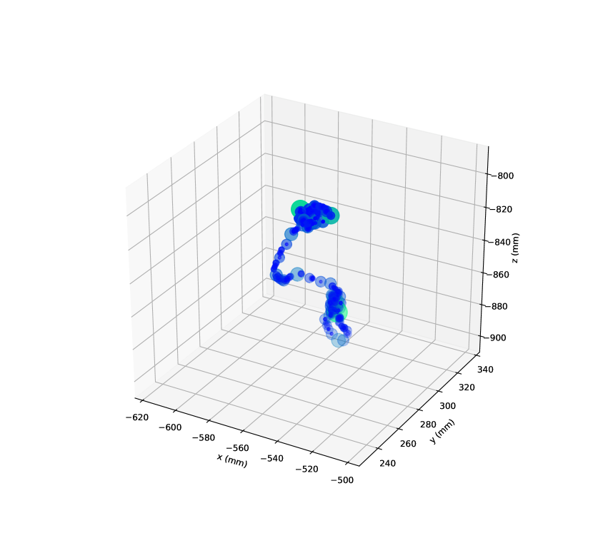
(a)

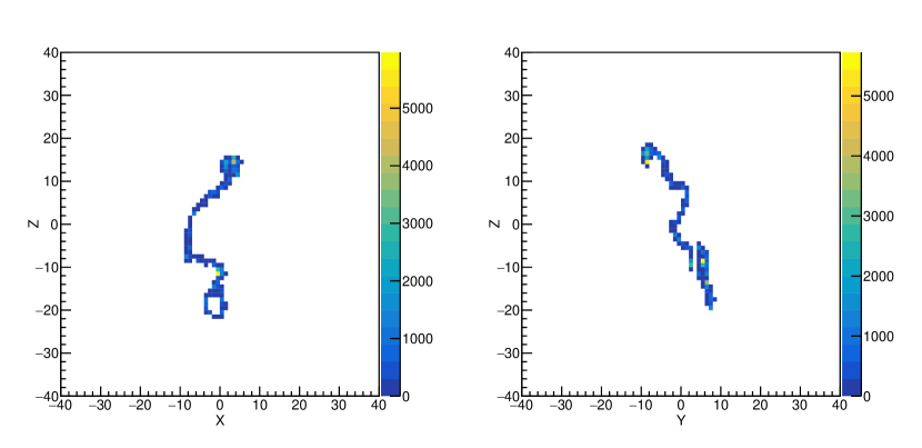
(b)

(c)

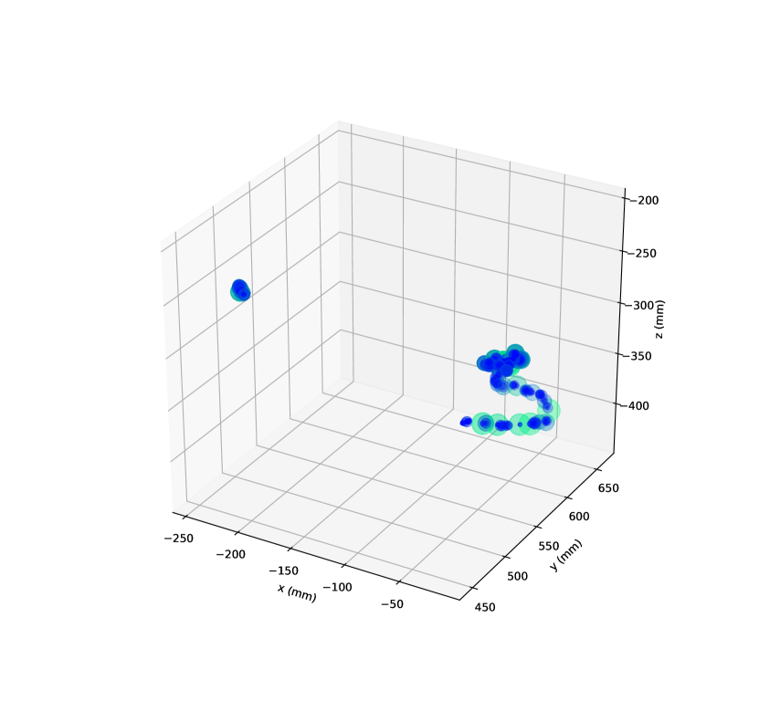
(d)

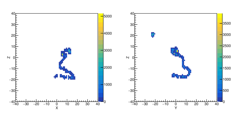
(e)

(f)

Figure 3: Examples of mapping from recorded events to images. Top: ¹³⁶Xe NLDBD event; Bottom: Gamma background event from ²¹⁴Bi. (a) and (d): The raw Monte Carlo 3D hits map. (b) and (e): The $x$-$z$ and $y$-$z$ projection of the event after reconstruction. (c) and (f): The resulting images for training. For better visualization, color inversion and enhancement were applied to the final images. The cyan color stands for the red channel, and the magenta color for the green channel.

We generated $5.6\times 10^{5}$ images from simulated NLDBD signal events and $5.6\times 10^{5}$ images from the high energy gamma background events. Within these images, $80\%$ (training set) are used for the training of the CNN, $10\%$ (validation set) are used for the validation, and remain $10\%$ (testing set) are used for the checking of the power of discrimination.

4.3 Results of Event Discrimination

The modified ResNet-50 was trained with the training set on a workstation with two NVidia GeForce 1080 GPUs for 30 epochs. To prevent overfitting and use the input data more efficiently, real-time data augmentation, such as the random operations of rotation, shifting and shearing, have been applied to the training images. The network parameters were updated in each epoch. The value of “accuracy”, defined as the ratio between the number of correctly recognized events over the total number of events with the threshold of 0.5, is a measurement of the agreement of model prediction in comparison with the data. We plot the training and validation accuracies in Fig. 4. The network became overfitting apparently after the 20th epoch due to the validation accuracy became smaller than the training accuracy, though the difference is small. The training accuracy and validation accuracy are nearly identical from the 16th to 20th epoch, and the relative differences are smaller than $0.1\%$. To avoid the bias introduced by the arbitrary selection of models, we used all the trained models from the 16th to 20th epochs in following study.

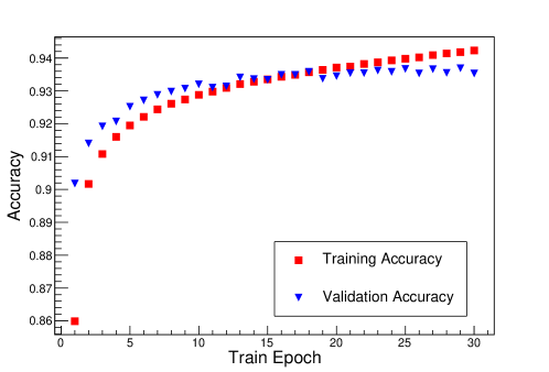
Figure 4: The evolution of the training/validation accuracy with epochs.

The trained models were used to classify the images in the testing set. For each input image, the output value $\kappa$ is a number between 0 and 1, representing how it looks like a background (0) and a signal (1). The distributions of $\kappa$ for NLDBD signal and backgrounds from model-16 (trained model in the 16th epoch) are shown in Fig. 5.

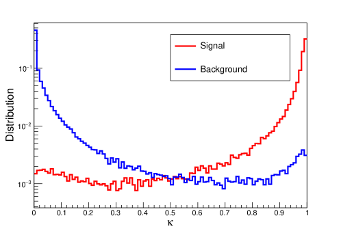
Figure 5: The distributions of $\kappa$ for NLDBD signals (red) and high energy gamma backgrounds (blue) from model-16 in testing dataset. The rising of $\kappa$ for backgrounds is resulted from the signal-like background events.

A cutting threshold can be applied on the distribution to obtain the signal and background efficiency. The efficiency curves for signal and background events of model-16 at different cut values are given in Fig. 6. The selection of the threshold can be optimized by the definition of figure of merit (FOM). The commonly defined FOM is proportional to the ratio between the final number of signal events $s$ and the square root of final number of background events $b$, or

$$\text{FOM}\propto\frac{s}{\sqrt{b}}=\frac{s_{d}}{\sqrt{b_{d}}}\cdot\frac{\epsilon_{s,cnn}}{\sqrt{\epsilon_{b,cnn}}}\propto\frac{\epsilon_{s,cnn}}{\sqrt{\epsilon_{b,cnn}}},$$ (1)

where $\epsilon_{s,cnn}$ and $\epsilon_{b,cnn}$ are the efficiencies for signal and background of CNN at a given cut $\kappa_{c}$, respectively, and $s_{d}$ and $b_{d}$ are the number of detected signal events and backgrounds before the CNN discrimination.

The optimized $\kappa_{c}$ can be found by maximizing the efficiencies ratio of $\epsilon_{s,cnn}/\sqrt{\epsilon_{b,cnn}}$. The efficiencies as functions of $\kappa_{c}$ from model-16 is plotted in Fig. 6. The background rejection efficiency versus signal efficiency is shown in Fig. 7. The corresponding signal and background efficiencies at optimized $\kappa_{c}$ in each model are given in Table. 2.

epoch	optimized $\kappa_{c}$	$\epsilon_{s,cnn}$	$1-\epsilon_{b,cnn}$	$\epsilon_{s,cnn}/\sqrt{\epsilon_{b,cnn}}$	final BI
16	0.983	0.475	0.9943	6.264	$1.775\times 10^{-5}$
17	0.976	0.569	0.9916	6.196	$2.605\times 10^{-5}$
18	0.981	0.487	0.9936	6.098	$1.968\times 10^{-5}$
19	0.966	0.540	0.9923	6.165	$2.369\times 10^{-5}$
20	0.976	0.520	0.9928	6.145	$2.215\times 10^{-5}$
average				$6.174\pm 0.055$

Table 2: The optimized $\kappa_{c}$, corresponding signal efficiency $\epsilon_{s,cnn}$, background rejection efficiency $1-\epsilon_{b,cnn}$, the ratio of $\epsilon_{s,cnn}/\sqrt{\epsilon_{b,cnn}}$ and final BI (count$\cdot$kg${}^{-1}\cdot$keV${}^{-1}\cdot$year^-1). The BI before the CNN discrimination is $3.088\times 10^{-3}$ count$\cdot$kg${}^{-1}\cdot$keV${}^{-1}\cdot$year^-1 [5].

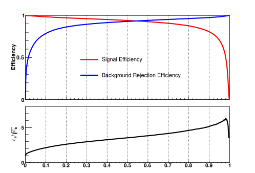
Figure 6: Top: The signal efficiency $\epsilon_{s,cnn}$ (red) and the background rejection efficiency $1-\epsilon_{b,cnn}$ (blue) as a function of $\kappa_{c}$ from model-16. Bottom: The efficiency ratio $\epsilon_{s,cnn}/\sqrt{\epsilon_{b,cnn}}$ as a function of $\kappa_{c}$ from model-16. The optimized $\kappa_{c}$ is plotted as a green dashed line.

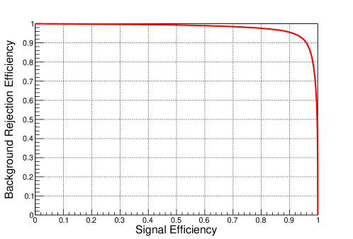
Figure 7: The background rejection efficiency $1-\epsilon_{b,cnn}$ versus the signal efficiency $\epsilon_{s,cnn}$ from model-16.

We obtained different signal efficiency and background rejection efficiency with the trained network in different epochs. The final background index has been suppressed by a factor larger than 100 in all the models. The relative error of the efficiency ratio $\epsilon_{s,cnn}/\sqrt{\epsilon_{b,cnn}}$ is only $0.09\%$, indicating the stability of the discrimination and should be treated as the systematic error from model selection. The reconstructed energy spectra of signal and background events before and after the optimal cut $\kappa_{c}$ from model-16 are plotted in Fig. 8. The shape of correctly identified signal events is similar to that before the classification.

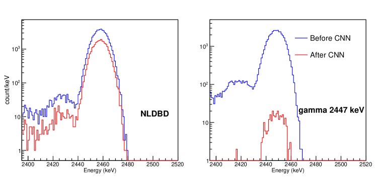
Figure 8: The reconstructed energy spectra of signal and backgrounds before and after the optimal cut $\kappa_{c}$ from model-16. left: NLDBD signal events; right: background events from ²¹⁴Bi. The spectra are not normalized.

Examples of falsely identified events are given in Fig. 9. The two expected Bragg peaks are not evident in the miss identified signal events. But in the falsely identified background, one could easily recognize relative large energy depositions at the two ends of the tracks.

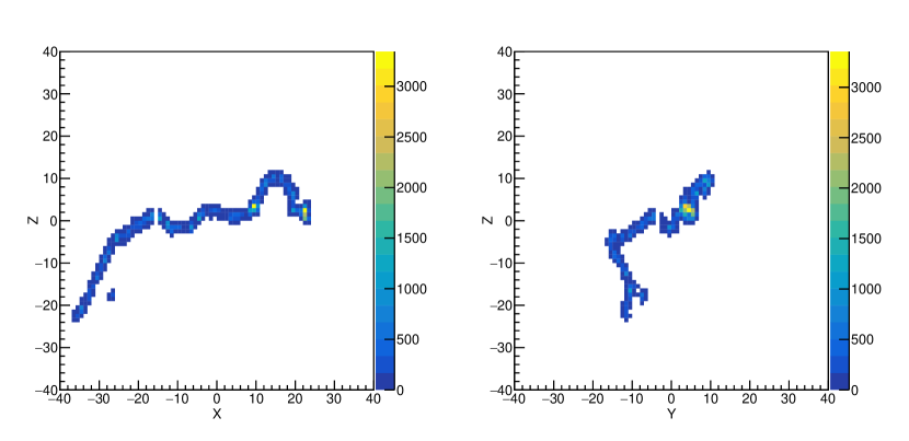
(a)

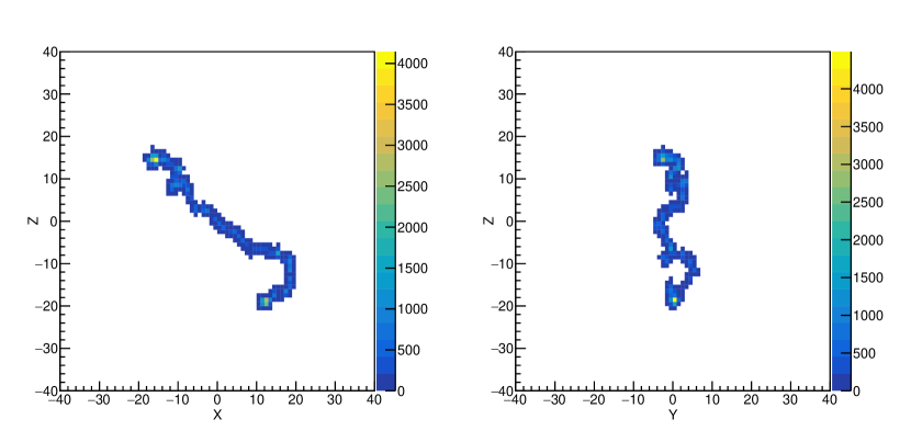
(b)

Figure 9: Falsely identified events by CNN in epoch 16. (a) The $x$-$z$ and $y$-$z$ projection of a NLDBD signal event, which is identified as a background event. (b): The $x$-$z$ and $y$-$z$ projection of a background event, which is identified as a signal event.

	PandaX-III baseline	CNN (model-16)	CNN (model-18)	CNN (average)
$\epsilon_{s}$	0.645	0.475	0.487
$1-\epsilon_{b}$	0.9714	0.9943	0.9936
$\epsilon_{s}/\sqrt{\epsilon_{b}}$	3.816	6.264	6.098	6.174
improvement	-	$64.2\%$	$59.8\%$	$61.8\%$

Table 3: Comparison between the results from PandaX-III baseline requirement and the CNN method.

We also generated a small dataset by simulating the high energy gamma resulting from the ²³⁸U and ²³²Th contamination in the steel bolts. Nearly identical background rejection power is achieved by applying the trained network to the dataset. That demonstrates that the initial position of background gamma has no visible effect on the discrimination power of CNN.

According to the PandaX-III CDR, the expected background suppression factor by the traditional topological method is 35. The comparison between it and the CNN method is given in Table. 4. The CNN method improves the efficiency ratio greatly, thus the detection sensitivity will be improved accordingly. The large number of parameters in the CNN method helps to describe the features of physical events better in comparison with the traditional methods.

5 Summary

We studied the method for the discrimination of signal and background with CNN in the PandaX-III experiment based on Monte Carlo simulation. By training a modified ResNet-50 model with digitized MC data which contains only the $x$-$z$ and $y$-$z$ snapshot information, we successfully achieved a relatively high efficiency ratio of $\epsilon_{s,cnn}/\sqrt{\epsilon_{b,cnn}}$, which improves the corresponding ratio from PandaX-III CDR with topological method by about $62\%$. Further studies are required to incorporate with the detector readout response, such as the signal formation for a better description of the experimental data.

Appendix A The ambiguity of position reconstruction with strip readout

The MicroMegas modules used by PandaX-III are read out with strips. Simultaneously hits on different strips can be used to reconstructed the positions of the signal. But ambiguity appears when more than 2 strips are fired at the same time, and an example is visualized in Fig. 10.

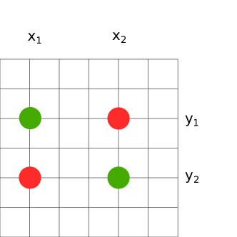
Figure 10: An example of the ambiguity in the position reconstruction with strip readout. The true positions of hits are $(x_{1},y_{1})$ and $(x_{2},y_{2})$ (green dots). Because all the $x_{1},x_{2},y_{1},y_{2}$ strips have been fired, additional fake hits of $(x_{1},y_{2})$ and $(x_{2},y_{2})$ may be reconstructed (red dots).

Appendix B Comparison between three CNN models

We have tested several different CNN structures for the discrimination of signal and background with a smaller training data set. A comparison between the model complexity, best training accuracy and the signal efficiency at a fixed background rejection efficiency for the testing data is given in Table 4. The ResNet-50 is finally chosen due to its highest signal efficiency.

Model	number of trainable parameters	accuracy	$\epsilon_{s}$
3-Layer Convolutional Model	$720,993$	$82\%$	$35.7\%$
VGG-16[27]	$15,894,849$	$92.8\%$	$73.9\%$
ResNet-50	$24,059,393$	$94.0\%$	$79.0\%$

Table 4: Simple comparison between different CNN models with a smaller training dataset. The signal efficiency $\epsilon_{s}$ is calculated at a fixed background rejection efficiency of $98.0\%$.

References

- [1] F. T. Avignone, III, S. R. Elliott, and J. Engel, Rev. Mod. Phys. 80, 481–516 (2008).
- [2] A. Gando et al. (The KamLAND-Zen collaboration), Phys. Rev. Lett. 117, 082503 (2016).
- [3] J. B. Albert et al. (The EXO-200 collaboration), Nature 510, 229–234 (2014).
- [4] V. Alvarez et al. (The NEXT collaboration), JINST 7, T06001 (2012).
- [5] X. Chen et al. (The PandaX-III collaboration), Sci. China Phys. Mech. Astron. 60, 061011 (2017).
- [6] S. Cebrián, T. Dafni, H. Gómez, D. C. Herrera, F. J. Iguaz, I. G. Irastorza, G. Luzón, L. Segui, and A. Tomás, J. Phys. G 40, 125203 (2013).
- [7] P. Ferrario et al. (The NEXT collaboration), JHEP 01, 104 (2016).
- [8] P. Baldi, K. Bauer, C. Eng, P. Sadowski, and D. Whiteson, Phys. Rev. D 93, 094034 (2016).
- [9] J. Barnard, E. N. Dawe, M. J. Dolan, and N. Rajcic, Phys. Rev. D 95, 014018 (2017).
- [10] A. Aurisano, A. Radovic, D. Rocco, A. Himmel, M. D. Messier, E. Niner, G. Pawloski, F. Psihas, A. Sousa, and P. Vahle, JINST 11, P09001 (2016).
- [11] P. T. Komiske, E. M. Metodiev, and M. D. Schwartz, JHEP 01, 110 (2017).
- [12] C. F. Madrazo, I. H. Cacha, L. L. Iglesias, and J. M. de Lucas, arXiv:1708.07034 (2017).
- [13] R. Haake, in 2017 European Physical Society Conference on High Energy Physics (EPS-HEP 2017) Venice, Italy, July 5-12 (2017), volume EPS-HEP2017, (2017).
- [14] H. Luo, M. Luo, K. Wang, T. Xu, and G. Zhu, arXiv:1712.03634 (2017)
- [15] J. Renner et al. (The NEXT collaboration), JINST 12, T01004 (2017).
- [16] X. Cao et al. (The PandaX-I collaboration), Sci. China Phys. Mech. Astron. 57, 1476–1494 (2014).
- [17] A. Tan et al. (The PandaX-II collaboration), Phys. Rev. D 93, 122009 (2016).
- [18] I. G. Irastorza et al. JCAP 1601, 033 (2016).
- [19] S. Agostinelli et al. Nucl. Instrum. Meth. A 506, 250–303 (2003).
- [20] J. Allison et al. (The GEANT4 collaboration), IEEE Trans. Nucl. Sci. 53, 270 (2006).
- [21] O. A. Ponkratenko, V. I. Tretyak, and Y. G. Zdesenko, Phys. Atom. Nucl. 63, 1282–1287 (2000).
- [22] E. Aprile and T. Doke, Rev. Mod. Phys. 82, 2053–2097 (2010).
- [23] http://magboltz.web.cern.ch/magboltz/,
- [24] https://garfieldpp.web.cern.ch/garfieldpp/,
- [25] A. Krizhevsky, I. Sutskever, and G. E. Hinton, in Advances in Neural Information Processing Systems 25, edited by F. Pereira, C. J. C. Burges, L. Bottou, and K. Q. Weinberger (Curran Associates, Inc. (2012)). pp. 1097–1105 (2012).
- [26] M. D. Zeiler and R. Fergus, CoRR, abs/1311.2901 (2013).
- [27] K. Simonyan and A. Zisserman, CoRR, abs/1409.1556 (2014).
- [28] K. He and J. Sun, CoRR, abs/1412.1710 (2014).
- [29] K. He, X. Zhang, S. Ren, and J. Sun, CoRR, abs/1512.03385 (2015).
- [30] F. Chollet et al. Keras, https://github.com/keras-team/keras (2015).