N-break states in a chain of nonlinear oscillators
Abstract
In the present work we explore a pre-stretched oscillator chain where the nodes interact via a pairwise Lennard-Jones potential. In addition to a homogeneous solution, we identify solutions with one or more (so-called) “breaks”, i.e., jumps. As a function of the canonical parameter of the system, namely the precompression strain , we find that the most fundamental one break solution changes stability when the monotonicity of the Hamiltonian changes with . We provide a proof for this (motivated by numerical computations) observation. This critical point separates stable and unstable segments of the one break branch of solutions. We find similar branches for 2 through 5 break branches of solutions. Each of these higher “excited state” solutions possesses an additional unstable pair of eigenvalues. We thus conjecture that break solutions will possess at least (and at most ) pairs of unstable eigenvalues. Our stability analysis is corroborated by direct numerical computations of the evolutionary dynamics.
I Introduction
The study of chains with pair-wise interaction potentials has had a long and distinguished history since the inception of the Fermi-Pasta-Ulam (FPU) model [1]; see for some relevant accounts the works of [2; 3]. Intriguingly, some of the original questions revolving around the foundations of associated studies remain active topics of investigation even half a century later. Among them, we note the potential equipartition of the energy among different degrees of freedom [4], or the number of solitary waves emerging in the early Kruskal-Zabusky simulations [5]; for the latter, see the associated recent work of [6].
In the present work, we intend to examine a variant of such inter-site interaction potential chains, in the context of a Lennard-Jones (LJ) potential [7]. We focus, in particular, on the equilibrium states of a pre-stretched, one-dimensional LJ chain and provide a detailed bifurcation analysis of the elastic (i.e., homogeneous) and broken states, where one or more bonds deviate towards large strains, rendering the chain inhomogeneous. We will use the terms broken or fractured to denote the latter bonds. The Lennard-Jones potential is prototypical of non-convex pair interactions, with a convex region for close particles and a concave region for longer-range interactions, with the force decaying to zero as the interparticle distance goes to infinity. The non-convexity allows the potential to model fractured states of the material, where two portions of the chain are sufficiently separated and have very weak interactions, as is done in -convergence approaches to the continuum limit of such 1D chains [8; 9].
Among the numerous and diverse topics considered for such LJ lattices, for example the dynamics and mean length of clusters at finite temperature [10], the (homoclinic to exponentially small periodic oscillations) subsonic, as well as (periodic) supersonic lattice traveling waves [11], the potential for chaotic motion through the maximum Lyapunov exponent [12], and as a model for superheated and stretched liquids [13] (whereby the role of the different dynamical configurations must be assessed in the calculation of thermodynamic quantities). A linear approximation of the chain and its solutions for nearest-neighbor (NN) and next-near neighbor (NNN) interactions was explored in [14].
The existence and stability of one break solutions was studied for the Morse [15] and LJ [13] potentials, while the instability of more than 1 break solutions was argued. This can be seen intuitively by considering the translation of a non-boundary segment in a direction that closes one of the fractures. In both cases the arguments used were based on the relative character of the energy minimum. In the latter study statistical mechanics arguments were used. Using the static solutions as initial states, these studies were extended in molecular dynamics methods to study the expected time for a failure to occur at finite temperatures (see, e.g., [16] and references therein), and collective fluctuations [17]. Later, it was shown that for a wide range of potentials and many-neighbor interactions, the chain with more than one fracture is always locally unstable [18] (see also references therein).
Our aim here is somewhat different, as we explore the bifurcation analysis of different states and provide a systematic count of the eigenvalues of the different branches of solutions. We also consider the eigendirections of the relevant instabilities and excite them in order to observe the dynamical response of the chain to different unstable perturbations (when appropriate). This helps us shape a systematic picture about the existence, stability and dynamical properties of the chain. It adds to the picture provided by molecular dynamics simulations by showing more direct paths to create broken chains, using eigendirections of the linear excitations.
Our presentation hereafter will be structured as follows. In Section II, we will present the mathematical formulation and some of the principal features of the model. In Section III, we will prove a basic result for the stability of the static solutions in connection to the monotonicity of the Hamiltonian as a function of the driving precompression parameter. In Section IV, we will present numerical computations of existence, stability and dynamics. Finally, in Section V, we will summarize our findings and present our conclusions, as well as some directions for future work.
II Mathematical Setup: Nearest-neighbor interaction between pre-stretched oscillators chain
We consider the following Hamiltonian system describing free oscillators interacting via a potential with the two ends clamped. Let for denote the displacements of the oscillators, with and We also assume that the chain has been pre-stretched to a separation value (Bold characters denote vectors whose components are as in ) The Hamiltonian is written as the sum of kinetic and potential energy, giving
From this we obtain the equations of motion
| (1) |
If we consider the interaction potential to be of the LJ type, scaled to have the dimensionless form:
| (2) |
the reference length, where force is zero, is at such that
| (3) |
Similarly, the inflection point is obtained from:
| (4) |
In our considerations within what follows, we will examine the possible solutions of the corresponding static problem as parametrized by . Once a static solution is identified we perturb them by means of the ansatz:
| (5) |
Substituting in the equation of motion, written as
| (6) |
we obtain
| (7) |
or
| (8) |
At we obtain the steady state equation, and at we have:
| (9) |
where is the Jacobian matrix. This is an eigenvalue problem arising for the eigenvalue-eigenvector pair . The relevant i-th pair will also be denoted by in what follows. Its result will allow us to assess the spectral (linear) stability of the different solutions, as a non-vanishing real part of the eigenvalue (positive ) will be associated with dynamical instability (the perturbation will grow), while for marginally stable solutions (the perturbation will just oscillate) all ’s will lie on the imaginary axis (negative ).
III Bifurcation analysis of the Lennard-Jones chain: A Criterion
Before we embark on a systematic numerical computation of the stationary solutions and their spectral properties, we establish a theoretical criterion for stability motivated by our numerical computations that will follow. Due to the nearest-neighbor interactions between the particles, the equilibrium states are particularly simple, as the balance of force on each particle gives
| (10) |
We define the bond length (or strain) variables where we have the equilibrium condition
The Dirichlet boundary conditions correspond to the total strain condition
| (11) |
We let For there are two solutions to one with , the other with We describe a bond with length as elastic and with length as broken, and define the two right inverses and where for every In the following, we will consider equilibria containing one or more breaks.
Lemma 1.
There is a minimal for which one break solutions exist, corresponding to isolated saddle points at which the stability of the equilibria changes.
Proof.
From the elastic and broken bond solutions, we can parameterize the equilibrium states using the bond stress Then, a uniformly stretched chain has total length whereas a chain with a single break has total length Note that is a monotone increasing function of , whereas is not, it has a local minimum when
The total energy for a chain with a single break is and we see
| (12) |
so that its local minimum corresponds to that of We can also show directly that this point represents a change in stability for the single fracture solution.
For that, consider a single-fracture equilibrium with strain where we take without loss of generality and for We will denote the internal stress We then consider the mean-zero perturbation direction
When applying a perturbation for positive this enlarges the break, proportionally shrinking the rest of the chain, and inversely for negative For large enough there are two single-fracture equilibria possible, one stable and one unstable, with the unstable branch moving toward the no break solution for negative epsilon and toward the stable single-fracture equilibrium for positive epsilon, see Figure 1 below. Then we expand the energy
The linear term in is zero since is an equilibrium. The quadratic coefficient satisfies
where the last equality follows from differentiating This has a zero (that is, a change of concavity) exactly when does as well. ∎
This calculation suggests that motion along this eigendirection becomes neutral as we cross the relevant critical point of the length or energy curve as a function of the precompression parameter . As a result, crossing this point will induce a change of stability along the corresponding eigendirection, a feature that we will monitor further in our detailed computations below. It is relevant to point out here that the stability criterion developed herein is in line with recent criteria (based on energy monotonicity changes upon suitable parametric variations) for stability of both traveling waves in lattices [19; 20] and breather-like periodic orbits [21].
Note that the criterion proved above is applicable to any potential that has a change of concavity and a maximum for the absolute value of the force.
IV Numerical results for the Nearest-Neighbor Lennard-Jones Potential
IV.1 Steady state
In our existence computations, we identified stationary solutions via a fixed point (Newton) iteration scheme. Using Eq. (9), we also calculate the eigenmodes and corresponding eigenvalues of that configuration (where the index in both and labels an ordering, which we choose to be of decreasing magnitude of ). Upon identifying a member of a particular family of solutions (with one or more breaks/fractures), we performed a continuation in the parameter . When a turning point was reached, the direction of variation of was reversed, and care was taken to ensure the segment of the curve followed was a different one (see Figs. (1–3)). A more detailed description of the numerical procedure can be found, e.g., in Ref. [22].
In what follows we will be showing results obtained for a chain with 20 free nodes.
IV.1.1 1 break
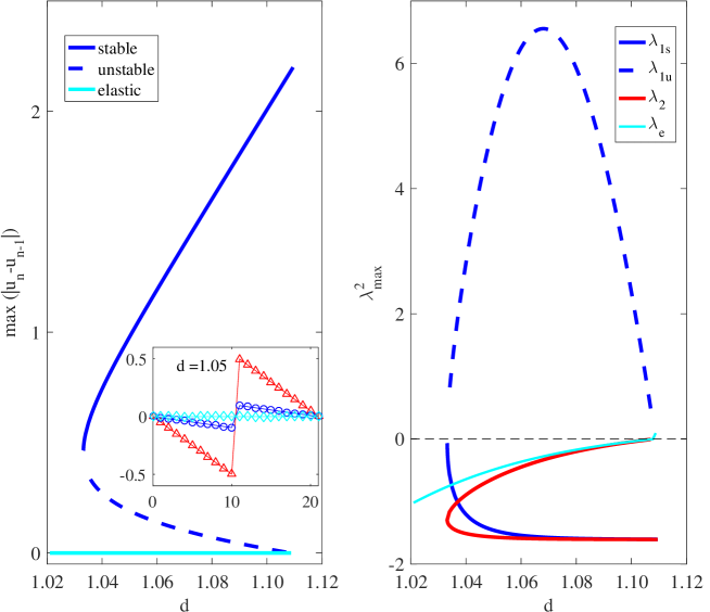
In Fig. 1, left panel, we have represented the amplitude of the broken bond as a function of the continuation parameter . Two modes were found, a stable (blue, solid), and an unstable one (blue, dashed). The elastic (no breaks) mode is also shown (cyan,solid). The inset shows the corresponding profiles for select values of . These broken states only exist above , the turning point of the branch. The unstable one break branch can also be identified in the graph as bifurcating from the uniform elastic solution at the critical strain
In the right panel we show the highest eigenvalue for each , and also the second highest if the mode is unstable. As per the analysis of the previous section, the monotonicity change of the maximal strain is correlated with the stability change of the one break solutions. We have indeed confirmed that the maximal strain, as well as the total length of the chain but also, importantly, the energy of the configuration all have turning points at the location of the change of stability of the branch. In particular, the monotonically increasing portion of the branch is associated with stability, while the monotonically decreasing one with instability. Let us now see how the situation is modified in the presence of an additional break.
IV.1.2 2 breaks

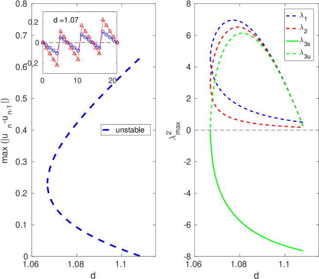
The configuration with 2 breaks was found to be always unstable; see Fig. 2. In this case too, the branch was found to possess two segments, one of which with two unstable eigenvalue pairs (the additional one stemming from the monotonicity of the energy as a function of the precompression strain ), while the other one with only one unstable eigenvalue pair. These two branch segments once again terminated in a saddle-center bifurcation at a critical value of , higher than that of the 1 break branch.
IV.1.3 3 breaks
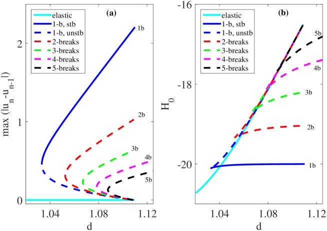
Similar conclusions could be drawn for the case with breaks; see Fig. 3. Here, the different segments of the branch generically possessed two unstable eigenvalue pairs. The one with the monotonically increasing dependence on had only these two unstable modes, while the decreasing one, just as before, featured an additional pair of unstable eigenvalues. From this, as well as our additional results involving modes up to breaks, a general picture is emerging regarding the stability properties of the different branches. As illustrated in section III, the change of monotonicity of the energy is associated with a change of stability of a particular eigenmode. For the relevant eigenmode, an increasing energy as a function of results in stability (along this eigendirection) while a decreasing energy leads to instability. In addition to this eigendirection, the presence of breaks implies the existence of an additional unstable eigenmodes. These features are summarized in Fig. 4 showcasing the dependence of the maximal strain as well as of the energy on the precompression strain . Now, we discuss the implications of the excitation of the corresponding unstable eigenvectors, as a preamble towards predicting the dynamical evolution of the associated instabilities.
IV.1.4 Geometry of the Principal Eigenmodes
Our aim in the present section is to explore the exact stationary solutions when the unstable eigenmodes are appended to them, in order to appreciate the paths that the system can take towards the decay of the unstable stationary states. The next series of plots show the modes found above together with the eigenvectors that are associated with their potential instabilities, as identified before. The right panels show a linear combination of the mode with a small perturbation in the form of each eigenvector represented on the left panels. In Fig. 5 and the following similar figures, the weight given to the perturbation was exaggerated for clarity. On the corresponding dynamical simulations, small weights were applied, consistent with the linear stability hypothesis behind the calculation leading to those eigenvectors. This is shown for the upper and lower segments of branches in the top and bottom rows, respectively.
.
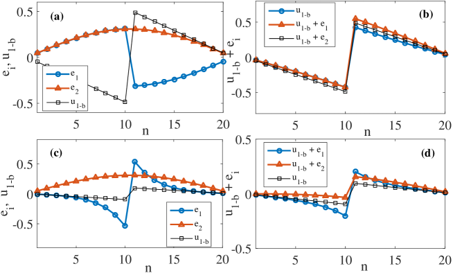
In Fig. 5 we show the effect of the eigenvector corresponding to the largest eigenvalue on the shape of the modes, for upper (linearly stable) and lower (unstable) single break branch segments. In this case we also show the second eigenvector for illustration, but it always has , so its effect will be oscillatory (i.e., the mode will be marginally stable and will not lead to instability). At first sight the eigenvectors seem to have opposite effects, but we can always perform a phase shift of (since there is the freedom of multiplying them by any real constant). The important difference lies on the sign of , which is negative for the upper branch segment, and so its effect is to solely lead to a benign oscillation, while for the lower branch segment it grows with time. It is this growth that leads to destruction of the mode. The decay can lead to 2 distinct results, as will be shown below: in the form shown, will make the unstable state (subscript for the lower segment branch and for the upper branch segment) grow towards a stable 1 break waveform on the upper branch segment, albeit a oscillating one, given the non-dissipative, Hamiltonian nature of the model. However, if we change the sign of the perturbation it will decay to the elastic mode, shedding some energy in the form of small amplitude waves in the process.
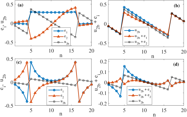
In Fig. 6 we show a similar representation for the 2 break case. The two leading eigenvectors alternate in parity with respect to the breaks, and so it is expected that they appear to seed different dynamical evolutions. For example, for the unstable lower branch, one of these eigendirections involves the two breaks moving in concert, either moving towards the larger 2 break solution or the uniform state.
On the other hand, addition of the other eigendirection (the one that is generically unstable) tends to convert the 2 break state into a 1 break one, i.e., to eliminate one of the two breaks. Similar interpretations can be generalized in the case of the 3 break solution, with the only difference that now there are two generically unstable eigendirections, tending to reduce the number of breaks in the system.
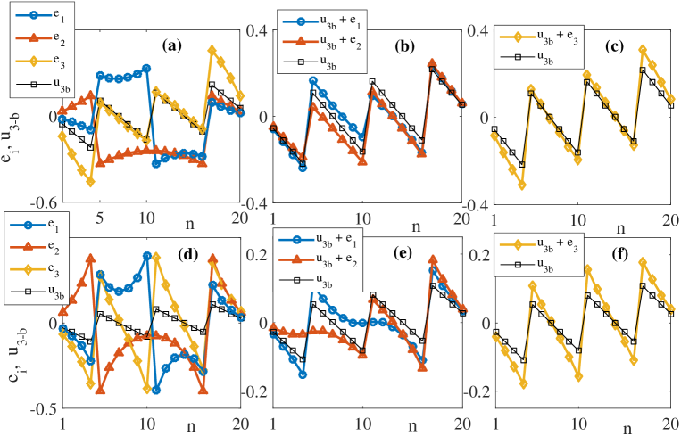
The analogous representation for the 3 break mode is shown in Fig. 7. Here, the most unstable eigenmode for the upper segment is either “in-phase” (IP) with the side breaks and “out-of-phase” (OOP) with the central one (as represented in left upper panel of the Fig. 7, blue circles) or vice-versa. This causes the elimination of the central break, allowing for the survival of the lateral ones, if added (as represented in the middle top panel of the same Fig. 7), or induces the decay the lateral ones, and survival of the one in the middle, that grows to a stable oscillating 1 break, if subtracted. The second most unstable eigenmode has a different parity (see again left upper panel, but now the red triangles), so it is natural to expect that whether added or subtracted will essentially lead to a qualitatively similar result. Again from the middle top panel, we see that it will initially reduce one of the lateral breaks, and increase the size of the other, the middle one remaining essentially unchanged. As for the third eigenmode, it is stable for this upper segment, i.e., will not lead to growth or decay, but only oscillation. From the right upper panel we see that its effect is more pronounced on the lateral breaks.
For the lower segment, from the lower left panel we can see that the general characteristics of the 3 eigenmodes represented do not differ from those of the upper segment. Given the smaller size of the mode of the lower segment, however, its effects can be more pronounced. This is apparent on the middle and right lower panels, where the central (for ), or left (for ) breaks have essentially disappeared. Now the third eigenvalue is also unstable. So the effects of the highest two eigenmodes should be qualitatively the same as for the upper segment. The third eigenvalue however, can show changes, as now it can lead to decay of all 3 breaks (if we have it OOP with the mode, i.e., oppositely to the situation represented).
We now turn to the dynamical evolution of the branches, armed with the interpretation of the different unstable states and their associated eigendirections.
IV.2 Dynamics
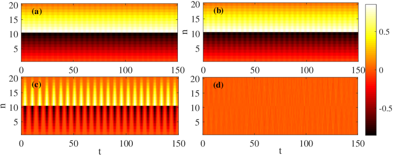
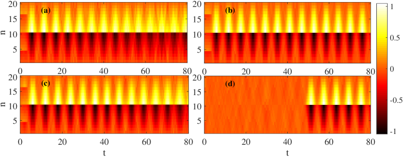
We start by illustrating the potential outcomes of the evolution of a 1 break state. In Fig. 8 we show the evolution of such a state at the value corresponding to the profiles shown in Fig. 5 i.e., for . On the upper row we start with an upper branch segment (stable) 1 break mode. We can see that, even with a moderate perturbation (in this case a component proportional to the eigenvector of the largest eigenvalue), the waveform is able to maintain its shape for the duration of the propagation, although there is some oscillation due to the extra energy stemming from the perturbation. We ensured that the numerical scheme conserved the initial energy throughout the propagation duration.
On the other end, the bottom panels show the evolution starting with the unstable 1 break solution for the same . Here the amount of perturbation introduced was much smaller (by an order of magnitude), and yet very quickly this 1 break decays. Importantly, however, the two distinct evolutions of panels (c) and (d) illustrate that depending on the direction of the perturbation, the unstable 1 break (operating as a separatrix) may lead either towards the stable 1 break branch segment (featuring large amplitude oscillations) or towards a homogeneous state. These two radically different behaviors shown in panels (c) and (d) confirm what was hinted on Fig. 5: adding the most unstable eigenvector takes the system to the stable 1 break solution, while subtracting takes it to the elastic state. It is interesting to point out that even without introducing any noise explicitly, the numerical round-off error would eventually lead the configuration to decay.
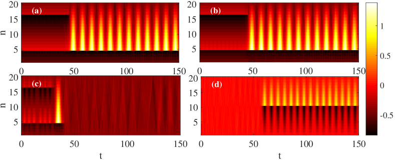
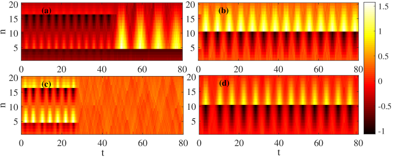
In Fig. 9 we represent now the result of propagation of a perturbed 2 break solution, corresponding to the profiles shown in Fig. 6, for which . The main difference now is that the highest eigenvalue is positive for both branch segments, and so it dominates the motion. As a result, although we perturb only with the second eigenvector (which is only unstable for the lower segment of the branch), even the upper branch segment suffers decay, because of numerical noise, although it takes longer to develop. Thus adding or subtracting the second eigenvector leads essentially to a (later) decay into a 1 break. For the lower branch adding should lead to an oscillation around an upper branch 2 break waveform, yet the effect of contamination by a causes one of them to decay. Subtracting should lead to an elastic mode, and that’s what the simulation shows during an initial stage. However the energy present is enough to eventually “nucleate” a stable 1 break.
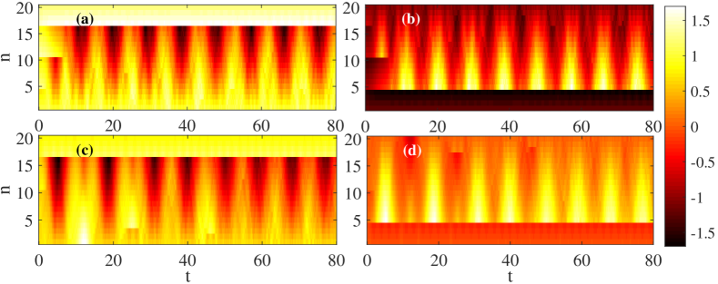
The scenario of the evolution of a perturbed 3 break is shown in Fig. 10-12. Here, as explained above, there are 2 unstable eigenvalues present for all elements of these branches of solutions. Therefore even more so than the 2 break case, the effects of are harder to see, as any numerical noise contamination introducing and/or will have stronger consequences. That is the reason why we chose to increase the strength of the perturbation here compared to the 1 and 2 break cases. The eigenvector is anti-symmetric like . For the lower segment of the branch, as noted before it will increase or decrease all breaks but more so the central one (as is larger there). So if added, the central break grows at the expense of the side ones to lead to a stable 1 break (left bottom panel of Fig. 10). If subtracted it will collapse all three breaks to the elastic mode, yet the extra energy will eventually allow the creation of a 1 break; right bottom panel of Fig. 10. Note that the decay happens very soon (), so it is hardly discernible in panel (d).
In the case of the upper segment of the branch its third eigenmode has a central “break” rather smaller than the side ones; see the left upper panel of Fig. 7. Thus, when added or subtracted to the stationary state, its influence is mainly on the side breaks, leading them to oscillate, given the negative sign of . This behavior, however, can only be seen for very short times. As previously mentioned, contamination with any of the lower eigenmodes, especially so the first which has the same parity, will lead to decay, governed mostly by those lower eigenmodes. This is evident on the dynamical simulation in the upper panels of Fig. 10.
Turning now to the influence of the stronger eigenmodes, notice that is IP with the side breaks but OOP with the central break. Then, in general, its effect will be to lead to the survival of the two side breaks by adding it, or the middle one by subtracting it. As we have seen before the 2 break is also unstable, so one of those two will later collapse as well (see e.g. the top left panel of Fig. 11). Notice the similarity between panel (b) and the upper panels of Fig. 10, pointing to the influence of in that case.
The effect of , on the other end, being an even mode is nearly the same whether we add or subtract it to the mode. From its shape, we can infer that it will collapse one of the side breaks, while increasing the other, and at an initial stage not influence much of the central one. But of course the 2 break thus formed is also unstable and one (the central one in this case) will soon disappear as well towards a 1 break state. This is confirmed in Fig. 12.
V Conclusions & Future Work
In the present work, we have examined solutions involving different numbers of fractures/breaks in a chain featuring a Lennard-Jones potential of interaction between the nodes and Dirichlet boundary conditions at the edges. We saw that for each of the solutions beyond the uniform, elastic one, there was a (more) stable and a (more) unstable portion of the branch, separated by a critical point where the monotonicity of the strain and/or the energy as a function of the precompression stress changed. At the same time, while the single break solutions could be potentially stable, any state with break would feature real eigenvalue pairs, being associated with respective instabilities. By monitoring the eigendirections of these instabilities, we could connect them with the tendency to eliminate one or more breaks from the chain and result to fewer break, more robust waveforms. These conclusions of the stability analysis were subsequently corroborated by means of direct numerical simulations featuring the unstable evolution of controlled numerical experiments where the instability-inducing eigenvectors were added to the unstable structures.
Naturally, a number of additional directions for future research are emerging as a result of the present study. On the one hand, in the one-dimensional setting, it is especially relevant to explore the role of interactions beyond those of nearest neighbors. Inducing next nearest neighbor interactions in competition with nearest neighbor ones may be a topic that will modify the stability of the presently considered states and will be of interest to explore in light of zigzag [23] and related configurations. On the other hand, it would be of particular interest to explore how configurations like the ones considered herein behave in higher dimensional settings. The latter offer the possibility of different types of geometries (e.g. in 2d square, hexagonal, honeycomb etc.) and thus may induce an interplay of geometry with the nonlinear interactions that may introduce novel states. Such studies are currently in progress and will be reported in future publications.
VI Aknowledgments
A.S.R. acknowledges financial support from FCT through grant UID/FIS/04650/2013, and grant SFRH/BSAB/135213/2017. PGK gratefully acknowledges support from the US-AFOSR under FA9550-17-1-0114, as well as from NSF-PHY-1602994.
References
- [1] E. Fermi, J. Pasta, and S. Ulam, Tech. Rep. Los Alamos Nat. Lab. LA1940 (1955).
- [2] D. K. Campbell, P. Rosenau, and G. M. Zaslavsky, Chaos 15, 015101 (2005).
- [3] G. Galavotti (Ed.) The Fermi-Pasta-Ulam Problem: A Status Report (Springer-Verlag, New York, 2008).
- [4] C. Danieli, D.K. Campbell, and S. Flach, Phys. Rev. E 95, 062002(R) (2017).
- [5] N.J. Zabusky, M.D. Kruskal, Phys. Rev. Lett. 15, 240–243 (1965).
- [6] G. Deng, G. Biondini, S. Trillo, Phys. D 333, 137–147 (2016).
- [7] J. E. Jones, Proc. R. Soc. Lond. A 106, 463–477 (1924).
- [8] A. Braides and M. Solci, Math. Mech. Solids 21, 915–930 (2016)
- [9] M. Schäffner and A. Schlömerkemper, arXiv:1501.06423v3 (2017).
- [10] G. R. Lee-Dadswell, N. Barrett, and M. Power, Phys. Rev. E 96, 032144 (2017).
- [11] C. Venney and J. Zimmer, Quart. Appl. Math. 72, 65–84 (2014).
- [12] T. Okabe, H. Yamada, and Masaki Goda, Phys. B 263-264, 445–447 (1999).
- [13] Frank H. Stillinger, Phys. Rev. E 52, 4685–4690 (1995).
- [14] M. Charlotte and L. Truskinovsky, J. Mech. Phys. Solids 50, 217–251 (2002).
- [15] Crist, B., Oddershede, J., Sabin, J.R., Perram, J.W. and Ratner, M.A., J. Polym. Sci. Polym. Phys. Ed., 22, 881-897 (1984).
- [16] F. A. Oliveira, Phys. Rev. B 57, 10576 (1998)
- [17] Lepri, S., Sandri, P. and Politi, A., Eur. Phys. J. B 47, 549 (2005).
- [18] C. Ortner and E. Süli, M2AN Math. Model. Numer. Anal. 42, 57–91 (2008).
- [19] J. Cuevas-Maraver, P.G. Kevrekidis, A. Vainchtein, and H. Xu, Phys. Rev. E 96, 032214 (2017).
- [20] H. Xu, J. Cuevas-Maraver, P.G. Kevrekidis, A. Vainchtein, arXiv:1711.03330.
- [21] P.G. Kevrekidis, J. Cuevas-Maraver, and D.E. Pelinovsky, Phys. Rev. Lett. 117, 094101 (2016).
- [22] P.G. Kevrekidis, The Discrete Nonlinear Schrödinger Equation: Mathematical Analysis, Numerical Computations and Physical Perspectives,(Springer, Berlin, Heidelberg 2009),chapters 2 and 9.
- [23] See, e.g., for an optical example of such an array: N.K. Efremidis and D.N. Christodoulides Phys. Rev. E 65, 056607 (2002).