Global stability of a distributed delayed viral model with general incidence rate

Eric Ávila-Vales 111Corresponding author: avila@correo.uady.mx , Abraham Canul-Pech and Erika Rivero-Esquivel
Universidad Autónoma de Yucatán, Facultad de Matemáticas
Anillo Periférico Norte, Tablaje 13615, C.P. 97119. Mérida, Yucatán, México.
Abstract

In this paper, we discussed an infinitely distributed delayed viral infection model with nonlinear immune response and general incidence rate. We proved the existence and uniqueness of the equilibria. By using the Lyapunov functional and LaSalle invariance principle, we obtained the conditions of global stabilities of the infection-free equilibrium, the immune-exhausted equilibrium and the endemic equilibrium. Numerical simulations are given to verify the analytical results.

keywords:
CTL-response , Lyapunov functional, basic reproduction number , viral reproduction number
MSC:
Primary: 34K20, secondary: 34D23

1 Introduction

During recent decades there has been a lot of research regarding mathematical modelling of viruses dynamics via models of ordinary differential equations (ODE). Advances in immunology have lead us to better understand the interactions between populations of virus and the immune system, therefore several nonlinear sytems of ordinary differential equations (ODE’s) has been proposed. Nowak and Bengham [1] study the model

x(t)superscript𝑥𝑡\displaystyle x^{\prime}(t) =sdx(t)βx(t)v(t),absent𝑠𝑑𝑥𝑡𝛽𝑥𝑡𝑣𝑡\displaystyle=s-dx(t)-\beta x(t)v(t), (1)
y(t)superscript𝑦𝑡\displaystyle y^{\prime}(t) =βx(t)v(t)ay(t)py(t)z(t),absent𝛽𝑥𝑡𝑣𝑡𝑎𝑦𝑡𝑝𝑦𝑡𝑧𝑡\displaystyle=\beta x(t)v(t)-ay(t)-py(t)z(t), (2)
v(t)superscript𝑣𝑡\displaystyle v^{\prime}(t) =ky(t)uv(t),absent𝑘𝑦𝑡𝑢𝑣𝑡\displaystyle=ky(t)-uv(t), (3)
z(t)superscript𝑧𝑡\displaystyle z^{\prime}(t) =cy(t)z(t)bz(t).absent𝑐𝑦𝑡𝑧𝑡𝑏𝑧𝑡\displaystyle=cy(t)z(t)-bz(t). (4)

Where x(t)𝑥𝑡x(t) denotes the number of healthy cells, y(t)𝑦𝑡y(t) denotes the infected cells, v(t)𝑣𝑡v(t) denotes the number of matures viruses and z(t)𝑧𝑡z(t) denotes the number of CTL (cytotoxic T lymphocyte response) cells. Uninfected target cells are assumed to be generated at a constant rate s𝑠s and die at rate d𝑑d. Infection of target cells by free virus is assumed to occur at rate β𝛽\beta. Infected cells die at rate a𝑎a and are removed at rate p𝑝p by the CTL immune response. New virus is produced from infected cells at rate k𝑘k and dies at rate u𝑢u. The average lifetime of uninfected cells, infected cells and free virus is thus given by 1/d1𝑑1/d, 1/a1𝑎1/a and 1/u1𝑢1/u, respectively. c𝑐c denotes rate at which the CTL response is produced, and b𝑏b denotes death rate of the CTL response, respectively, with all given constants positive.

Generally, the type of incidence function used in a model has an important role in modeling the dynamics of viruses. The most common, is the bilinear incidence rate βxv𝛽𝑥𝑣\beta xv. However, this rate is not useful all the time. For instance, using bilinear incidence suggests that model can not describe the infection process of hepatitis B, where individuals with small liver are more resistant to infection than the ones with a bigger liver. Recently, works about models of infections by viruses have used the incidence function of type Beddington-DeAngelis and Crowley-Martin. In [2] the authors propose a model of infection by virus with Crowley-Martin functional response βx(t)v(t)(1+ax(t))(1+bv(t))𝛽𝑥𝑡𝑣𝑡1𝑎𝑥𝑡1𝑏𝑣𝑡\frac{\beta x(t)v(t)}{(1+ax(t))(1+bv(t))}. Li and Fu in [3] study the following system:

x(t)superscript𝑥𝑡\displaystyle x^{\prime}(t) =sdx(t)βx(t)v(t)(1+ax(t))(1+bv(t)),absent𝑠𝑑𝑥𝑡𝛽𝑥𝑡𝑣𝑡1𝑎𝑥𝑡1𝑏𝑣𝑡\displaystyle=s-dx(t)-\frac{\beta x(t)v(t)}{(1+ax(t))(1+bv(t))}, (5)
y(t)superscript𝑦𝑡\displaystyle y^{\prime}(t) =βx(tτ)v(t)esτ(1+ax(tτ))(1+bv(tτ))ay(t)py(t)z(t),absent𝛽𝑥𝑡𝜏𝑣𝑡superscript𝑒𝑠𝜏1𝑎𝑥𝑡𝜏1𝑏𝑣𝑡𝜏𝑎𝑦𝑡𝑝𝑦𝑡𝑧𝑡\displaystyle=\frac{\beta x(t-\tau)v(t)e^{-s\tau}}{(1+ax(t-\tau))(1+bv(t-\tau))}-ay(t)-py(t)z(t), (6)
v(t)superscript𝑣𝑡\displaystyle v^{\prime}(t) =ky(t)uv(t),absent𝑘𝑦𝑡𝑢𝑣𝑡\displaystyle=ky(t)-uv(t), (7)
z(t)superscript𝑧𝑡\displaystyle z^{\prime}(t) =cy(t)z(t)bz(t).absent𝑐𝑦𝑡𝑧𝑡𝑏𝑧𝑡\displaystyle=cy(t)z(t)-bz(t). (8)

They construct a Lyapunov functional to establish the global dynamics of the system.

More recently, in [4], the authors consider the system

x(t)superscript𝑥𝑡\displaystyle x^{\prime}(t) =sdx(t)βx(t)v(t)1+ax(t)+bv(t),absent𝑠𝑑𝑥𝑡𝛽𝑥𝑡𝑣𝑡1𝑎𝑥𝑡𝑏𝑣𝑡\displaystyle=s-dx(t)-\frac{\beta x(t)v(t)}{1+ax(t)+bv(t)}, (9)
y(t)superscript𝑦𝑡\displaystyle y^{\prime}(t) =βx(t)v(t)1+ax(t)+bv(t)ay(t)py(t)z(t),absent𝛽𝑥𝑡𝑣𝑡1𝑎𝑥𝑡𝑏𝑣𝑡𝑎𝑦𝑡𝑝𝑦𝑡𝑧𝑡\displaystyle=\frac{\beta x(t)v(t)}{1+ax(t)+bv(t)}-ay(t)-py(t)z(t), (10)
v(t)superscript𝑣𝑡\displaystyle v^{\prime}(t) =ky(t)uv(t),absent𝑘𝑦𝑡𝑢𝑣𝑡\displaystyle=ky(t)-uv(t), (11)
z(t)superscript𝑧𝑡\displaystyle z^{\prime}(t) =cy(tτ)z(tτ)bz(t).absent𝑐𝑦𝑡𝜏𝑧𝑡𝜏𝑏𝑧𝑡\displaystyle=cy(t-\tau)z(t-\tau)-bz(t). (12)

They give also results of global stability as well as Hopf bifurcation results.

Yang and Wei in [5] consider a more general incidence rate, they study the system

x(t)superscript𝑥𝑡\displaystyle x^{\prime}(t) =sdx(t)x(t)f(v(t)),absent𝑠𝑑𝑥𝑡𝑥𝑡𝑓𝑣𝑡\displaystyle=s-dx(t)-x(t)f(v(t)), (13)
y(t)superscript𝑦𝑡\displaystyle y^{\prime}(t) =x(t)f(v(t))ay(t)py(t)z(t),absent𝑥𝑡𝑓𝑣𝑡𝑎𝑦𝑡𝑝𝑦𝑡𝑧𝑡\displaystyle=x(t)f(v(t))-ay(t)-py(t)z(t), (14)
v(t)superscript𝑣𝑡\displaystyle v^{\prime}(t) =ky(t)uv(t),absent𝑘𝑦𝑡𝑢𝑣𝑡\displaystyle=ky(t)-uv(t), (15)
z(t)superscript𝑧𝑡\displaystyle z^{\prime}(t) =cy(t)z(t)bz(t),absent𝑐𝑦𝑡𝑧𝑡𝑏𝑧𝑡\displaystyle=cy(t)z(t)-bz(t), (16)

giving some results about global stability in terms of the basic reproduction number and the immune response reproduction number. Here the f(v)𝑓𝑣f(v) is assumed to be a continuous function on v𝑣v that belongs to (0,)0(0,\infty) and satisfies f(0)=0,f(v)>0formulae-sequence𝑓00superscript𝑓𝑣0f(0)=0,f^{\prime}(v)>0 for all v𝑣v greater or equal to 0 and f′′(v)<0superscript𝑓′′𝑣0f^{\prime\prime}(v)<0 for all v𝑣v greater or equal to 00.

In [6] the authors consider a more general incidence rate f(x,y,v)v𝑓𝑥𝑦𝑣𝑣f(x,y,v)v, where f𝑓f is assumed to be continuously differentiable in the interior of +3subscriptsuperscript3\mathbb{R}^{3}_{+} and satisfies the following hypotheses

  • i)

    f(0,y,v)=0𝑓0𝑦𝑣0f(0,y,v)=0, for all y0𝑦0y\geq 0, v0𝑣0v\geq 0.

  • ii)

    fx(x,y,v)>0𝑓𝑥𝑥𝑦𝑣0\frac{\partial f}{\partial x}(x,y,v)>0 for all x>0𝑥0x>0, y>0𝑦0y>0, v>0𝑣0v>0.

  • iii)

    fy(x,y,v)0𝑓𝑦𝑥𝑦𝑣0\frac{\partial f}{\partial y}(x,y,v)\leq 0 and fv(x,y,v)0𝑓𝑣𝑥𝑦𝑣0\frac{\partial f}{\partial v}(x,y,v)\leq 0 for all x0𝑥0x\geq 0, y0𝑦0y\geq 0, v0𝑣0v\geq 0.

Finally, in [7] analyse an infection model by virus , with general incidence and immune response, which generalizes the systems by [2, 6, 8]:

x˙˙𝑥\displaystyle\dot{x} =sdxf(x,y,v)v,absent𝑠𝑑𝑥𝑓𝑥𝑦𝑣𝑣\displaystyle=s-dx-f(x,y,v)v,
y˙˙𝑦\displaystyle\dot{y} =f(x,y,v)vaypyz,absent𝑓𝑥𝑦𝑣𝑣𝑎𝑦𝑝𝑦𝑧\displaystyle=f(x,y,v)v-ay-pyz,
v˙˙𝑣\displaystyle\dot{v} =kyuv,absent𝑘𝑦𝑢𝑣\displaystyle=ky-uv,
z˙˙𝑧\displaystyle\dot{z} =cyzbz,absent𝑐𝑦𝑧𝑏𝑧\displaystyle=cyz-bz,

where f(x,y,v)𝑓𝑥𝑦𝑣f(x,y,v) is a continuous and differentiable function in the interior of +3superscriptsubscript3\mathbb{R}_{+}^{3} and satisfies the conditions [i)], [ii) [iii)].

Another viral infection model is the studied in [9] given by:

x˙˙𝑥\displaystyle\dot{x} =n(x)h(x,v),absent𝑛𝑥𝑥𝑣\displaystyle=n(x)-h(x,v),
y˙˙𝑦\displaystyle\dot{y} =0f1(τ)h(x(tτ),v(tτ))𝑑τag1(y)pw(y,z),absentsuperscriptsubscript0subscript𝑓1𝜏𝑥𝑡𝜏𝑣𝑡𝜏differential-d𝜏𝑎subscript𝑔1𝑦𝑝𝑤𝑦𝑧\displaystyle=\int_{0}^{\infty}f_{1}(\tau)h(x(t-\tau),v(t-\tau))d\tau-ag_{1}(y)-pw(y,z),
v˙˙𝑣\displaystyle\dot{v} =k0f2(τ)g1(y(tτ))𝑑τ,absent𝑘superscriptsubscript0subscript𝑓2𝜏subscript𝑔1𝑦𝑡𝜏differential-d𝜏\displaystyle=k\int_{0}^{\infty}f_{2}(\tau)g_{1}(y(t-\tau))d\tau,
z˙˙𝑧\displaystyle\dot{z} =c0f3(τ)w(y(tτ),z(tτ))𝑑τbg3(z).absent𝑐superscriptsubscript0subscript𝑓3𝜏𝑤𝑦𝑡𝜏𝑧𝑡𝜏differential-d𝜏𝑏subscript𝑔3𝑧\displaystyle=c\int_{0}^{\infty}f_{3}(\tau)w(y(t-\tau),z(t-\tau))d\tau-bg_{3}(z).

Where x,y,v,z𝑥𝑦𝑣𝑧x,y,v,z denotes the non infected cells, infected cells, virus and specific virus CTL at time t𝑡t, respectively. Conditions on functions fisubscript𝑓𝑖f_{i},h,w,𝑤h,w, and gisubscript𝑔𝑖g_{i} are specified in [9]. A related work is [10].

Based on the discussion above, we will study a delayed viral infection model with general incidence rate and CTL immune response given by

x˙˙𝑥\displaystyle\dot{x} =n(x)f(x(t),y(t),v(t))v(t),absent𝑛𝑥𝑓𝑥𝑡𝑦𝑡𝑣𝑡𝑣𝑡\displaystyle=n(x)-f(x(t),y(t),v(t))v(t), (17)
y˙˙𝑦\displaystyle\dot{y} =0f1(τ)f(x(tτ),y(tτ),v(tτ))v(tτ)eα1τ𝑑τaφ1(y(t))pw(y(t),z(t)),absentsubscriptsuperscript0subscript𝑓1𝜏𝑓𝑥𝑡𝜏𝑦𝑡𝜏𝑣𝑡𝜏𝑣𝑡𝜏superscript𝑒subscript𝛼1𝜏differential-d𝜏𝑎subscript𝜑1𝑦𝑡𝑝𝑤𝑦𝑡𝑧𝑡\displaystyle=\int^{\infty}_{0}f_{1}(\tau)f(x(t-\tau),y(t-\tau),v(t-\tau))v(t-\tau)e^{-\alpha_{1}\tau}d\tau-a\varphi_{1}(y(t))-pw(y(t),z(t)), (18)
v˙˙𝑣\displaystyle\dot{v} =k0f2(τ)eα2τφ1(y(tτ))𝑑τuv(t),absent𝑘subscriptsuperscript0subscript𝑓2𝜏superscript𝑒subscript𝛼2𝜏subscript𝜑1𝑦𝑡𝜏differential-d𝜏𝑢𝑣𝑡\displaystyle=k\int^{\infty}_{0}f_{2}(\tau)e^{-\alpha_{2}\tau}\varphi_{1}(y(t-\tau))d\tau-uv(t), (19)
z˙˙𝑧\displaystyle\dot{z} =c0f3(τ)w(y(tτ),z(tτ))𝑑τbφ2(z(t)).absent𝑐subscriptsuperscript0subscript𝑓3𝜏𝑤𝑦𝑡𝜏𝑧𝑡𝜏differential-d𝜏𝑏subscript𝜑2𝑧𝑡\displaystyle=c\int^{\infty}_{0}f_{3}(\tau)w(y(t-\tau),z(t-\tau))d\tau-b\varphi_{2}(z(t)). (20)

The dynamics of uninfected cells, x𝑥x, in absence of infection is governed by x=n(x),superscript𝑥𝑛𝑥x^{\prime}=n(x), where n(x)𝑛𝑥n(x) is the intrinsic growth rate of uninfected cells accounting for both productions and natural mortality, which is assumed to satisfy the following:

  • H1)H_{1})

    n(x)𝑛𝑥n(x) is continuously differentiable, and exist x¯>0¯𝑥0\bar{x}>0 such as that n(x¯)=0𝑛¯𝑥0n(\bar{x})=0, n(x)>0𝑛𝑥0n(x)>0 for x[0,x¯)𝑥0¯𝑥x\in[0,\bar{x}), and n(x)<0𝑛𝑥0n(x)<0 for x<x¯𝑥¯𝑥x<\bar{x}. Typical functions appearing in the literature are n(x)=sdx𝑛𝑥𝑠𝑑𝑥n(x)=s-dx and n(x)=sdx+rx(1x/xmax)𝑛𝑥𝑠𝑑𝑥𝑟𝑥1𝑥subscript𝑥𝑚𝑎𝑥n(x)=s-dx+rx\left(1-{x}/{x_{max}}\right).

  • H2)H_{2})

    φisubscript𝜑𝑖\varphi_{i} is strictly increasing on [0,)0[0,\infty); φi(0)=0subscript𝜑𝑖00\varphi_{i}(0)=0; φi(0)=1superscriptsubscript𝜑𝑖01\varphi_{i}^{\prime}(0)=1;limyφi(y)=+subscript𝑦subscript𝜑𝑖𝑦\lim_{y\longrightarrow\infty}\varphi_{i}(y)=+\infty; and exist ki>0subscript𝑘𝑖0k_{i}>0 such as φi(y)kiysubscript𝜑𝑖𝑦subscript𝑘𝑖𝑦\varphi_{i}(y)\geq k_{i}y for any yi0subscript𝑦𝑖0y_{i}\geq 0.

  • H3)H_{3})

    w(y,z)𝑤𝑦𝑧w(y,z) is continuously differentiable; w(y,z)z>0𝑤𝑦𝑧𝑧0\frac{\partial w(y,z)}{\partial z}>0 for y(0,)𝑦0y\in(0,\infty), z[0,)𝑧0z\in[0,\infty); w(y,z)>0𝑤𝑦𝑧0w(y,z)>0 for y(0,)𝑦0y\in(0,\infty) and z(0,)𝑧0z\in(0,\infty) with w(y,z)=0𝑤𝑦𝑧0w(y,z)=0 if and if only y=0𝑦0y=0 or z=0𝑧0z=0.

All parameters are nonnegative and the distributions fisubscript𝑓𝑖f_{i} for i=1,2𝑖12i=1,2 are assumed to satisfy the following (see [9] and [11] ) :

  • 1.

    fi(τ)0,forτ0formulae-sequencesubscript𝑓𝑖𝜏0for𝜏0f_{i}(\tau)\geq 0,\text{for}\hskip 7.22743pt\tau\geq 0.

  • 2.

    0fi(τ)𝑑τ=1superscriptsubscript0subscript𝑓𝑖𝜏differential-d𝜏1\int_{0}^{\infty}f_{i}(\tau)d\tau=1 for i=1,2𝑖12i=1,2.

  • 3.

    0f3(τ)𝑑τ1superscriptsubscript0subscript𝑓3𝜏differential-d𝜏1\int_{0}^{\infty}f_{3}(\tau)d\tau\leq 1 and 0f3(τ)esτ𝑑τ<superscriptsubscript0subscript𝑓3𝜏superscript𝑒𝑠𝜏differential-d𝜏\int_{0}^{\infty}f_{3}(\tau)e^{s\tau}d\tau<\infty for some s>0𝑠0s>0.

However, the uniqueness and Global stability results on the positive equilibrium require the following assumption.

  • H4)H_{4})

    w(y,z)=φ1(y)φ2(z)𝑤𝑦𝑧subscript𝜑1𝑦subscript𝜑2𝑧w(y,z)=\varphi_{1}(y)\varphi_{2}(z).

Motivated by the work mentioned above we consider the following model

x˙˙𝑥\displaystyle\dot{x} =n(x)f(x(t),y(t),v(t))v(t),absent𝑛𝑥𝑓𝑥𝑡𝑦𝑡𝑣𝑡𝑣𝑡\displaystyle=n(x)-f(x(t),y(t),v(t))v(t), (21)
y˙˙𝑦\displaystyle\dot{y} =0f1(τ)f(x(tτ),y(tτ),v(tτ))v(tτ)eα1τ𝑑τaφ1(y(t))pφ1(y(t))φ2(z(t)),absentsubscriptsuperscript0subscript𝑓1𝜏𝑓𝑥𝑡𝜏𝑦𝑡𝜏𝑣𝑡𝜏𝑣𝑡𝜏superscript𝑒subscript𝛼1𝜏differential-d𝜏𝑎subscript𝜑1𝑦𝑡𝑝subscript𝜑1𝑦𝑡subscript𝜑2𝑧𝑡\displaystyle=\int^{\infty}_{0}f_{1}(\tau)f(x(t-\tau),y(t-\tau),v(t-\tau))v(t-\tau)e^{-\alpha_{1}\tau}d\tau-a\varphi_{1}(y(t))-p\varphi_{1}(y(t))\varphi_{2}(z(t)), (22)
v˙˙𝑣\displaystyle\dot{v} =k0f2(τ)eα2τφ1(y(tτ))𝑑τuv(t),absent𝑘subscriptsuperscript0subscript𝑓2𝜏superscript𝑒subscript𝛼2𝜏subscript𝜑1𝑦𝑡𝜏differential-d𝜏𝑢𝑣𝑡\displaystyle=k\int^{\infty}_{0}f_{2}(\tau)e^{-\alpha_{2}\tau}\varphi_{1}(y(t-\tau))d\tau-uv(t), (23)
z˙˙𝑧\displaystyle\dot{z} =c0f3(τ)φ1(y(tτ))φ2(z(tτ))𝑑τbφ2(z(t)).absent𝑐subscriptsuperscript0subscript𝑓3𝜏subscript𝜑1𝑦𝑡𝜏subscript𝜑2𝑧𝑡𝜏differential-d𝜏𝑏subscript𝜑2𝑧𝑡\displaystyle=c\int^{\infty}_{0}f_{3}(\tau)\varphi_{1}(y(t-\tau))\varphi_{2}(z(t-\tau))d\tau-b\varphi_{2}(z(t)). (24)

In this paper, we will study the global dynamics model of (21), organization is as follows: in section 2, we prove the existence and uniqueness of the infection free equilibrium, the CTL-inactivated infection equilibrium and the CTL-activated infection equilibrium. In section 3, the conditions that allow the global stability of each equilibrium are determined and proved. Section 4 provide several numerical simulations that shows the results obtained in section 3 and 4. Finally, in section 5 we summarize the results obtained, comparing them with the previous models studied in literature, and setting the guidelines for possible future work.

1.1 Positivity and Boundedness

For system (21) the suitable space is 𝒞4=𝒞×𝒞×𝒞×𝒞superscript𝒞4𝒞𝒞𝒞𝒞\mathcal{C}^{4}=\mathcal{C}\times\mathcal{C}\times\mathcal{C}\times\mathcal{C}, where 𝒞𝒞\mathcal{C} is the Banach space of fading memory type ([12]):

C:={ϕC((,0],),ϕ(θ)eαθis uniformly continous forθ(,0]andϕ<},assign𝐶formulae-sequenceitalic-ϕ𝐶0italic-ϕ𝜃superscript𝑒𝛼𝜃is uniformly continous for𝜃0andnormitalic-ϕC:=\{\phi\in C((-\infty,0],\mathbb{R}),\hskip 7.22743pt\phi(\theta)e^{\alpha\theta}\hskip 7.22743pt\text{is uniformly continous for}\hskip 7.22743pt\theta\in(-\infty,0]\hskip 7.22743pt\text{and}\hskip 7.22743pt\|\phi\|<\infty\},

where α>0𝛼0\alpha>0 is a constant and the norm of a ϕ𝒞italic-ϕ𝒞\phi\in\mathcal{C} is defined as ϕ=supθ0|ϕ(θ)|eαθ.normitalic-ϕsubscriptsupremum𝜃0italic-ϕ𝜃superscript𝑒𝛼𝜃\|\phi\|=\sup_{\theta\leq 0}|\phi(\theta)|e^{\alpha\theta}. The nonnegative cone of 𝒞𝒞\mathcal{C} is defined as 𝒞+=C((,0],+)subscript𝒞𝐶0subscript\mathcal{C}_{+}=C((-\infty,0],\mathbb{R}_{+}).

Theorem 1.

Under the initial conditions, all solutions of system (21) are positive and ultimately uniformly bounded in X𝑋X.

Proof.

To see that x(t)𝑥𝑡x(t) is positive, we proceed by contradiction. Let t1subscript𝑡1t_{1} the first value of time such that x(t1)=0𝑥subscript𝑡10x(t_{1})=0. From the first equation of (21) we see that x(t1)=n(0)>0superscript𝑥subscript𝑡1𝑛00x^{\prime}(t_{1})=n(0)>0 and x(t1)=0𝑥subscript𝑡10x(t_{1})=0, therefore there exists ϵ>0italic-ϵ0\epsilon>0 such that x(t)<0𝑥𝑡0x(t)<0 for t(t1ϵ,t1)𝑡subscript𝑡1italic-ϵsubscript𝑡1t\in(t_{1}-\epsilon,t_{1}), this leads to a contradiction. It follows that x(t)𝑥𝑡x(t) is always positive. With a similar argument we see that y(t)𝑦𝑡y(t), v(t)𝑣𝑡v(t) and z(t)𝑧𝑡z(t) are positive for t0𝑡0t\geq 0.

The hypotheses (H1subscript𝐻1H_{1}) and first equation of (21) imply that lim suptx(t)x¯subscriptlimit-supremum𝑡𝑥𝑡¯𝑥\limsup_{t\longrightarrow\infty}x(t)\leq\bar{x}.
From two first equations of (21) and assumption (H2subscript𝐻2H_{2}), we obtain

0f1(τ)eα1τx(tτ)𝑑τ+y(t)=0f1(τ)eα1τn(x(tτ))𝑑τaφ1(y)M1G1ak1y,subscriptsuperscript0subscript𝑓1𝜏superscript𝑒subscript𝛼1𝜏superscript𝑥𝑡𝜏differential-d𝜏superscript𝑦𝑡subscriptsuperscript0subscript𝑓1𝜏superscript𝑒subscript𝛼1𝜏𝑛𝑥𝑡𝜏differential-d𝜏𝑎subscript𝜑1𝑦subscript𝑀1subscript𝐺1𝑎subscript𝑘1𝑦\int^{\infty}_{0}f_{1}(\tau)e^{-\alpha_{1}\tau}x^{\prime}(t-\tau)d\tau+y^{\prime}(t)=\int^{\infty}_{0}f_{1}(\tau)e^{-\alpha_{1}\tau}n(x(t-\tau))d\tau-a\varphi_{1}(y)\leq M_{1}G_{1}-ak_{1}y, (25)

where M1=supx[0,x¯]n(x)subscript𝑀1subscriptsupremum𝑥0¯𝑥𝑛𝑥M_{1}=\sup_{x\in[0,\bar{x}]}n(x) and G1=0f1(τ)eα1τ𝑑τsubscript𝐺1subscriptsuperscript0subscript𝑓1𝜏superscript𝑒subscript𝛼1𝜏differential-d𝜏G_{1}=\int^{\infty}_{0}f_{1}(\tau)e^{-\alpha_{1}\tau}d\tau.

Let e(t)=0f1(τ)eα1τx(tτ)𝑑τ𝑒𝑡subscriptsuperscript0subscript𝑓1𝜏superscript𝑒subscript𝛼1𝜏𝑥𝑡𝜏differential-d𝜏e(t)=\int^{\infty}_{0}f_{1}(\tau)e^{-\alpha_{1}\tau}x(t-\tau)d\tau. Then for e(t)x¯G1𝑒𝑡¯𝑥subscript𝐺1e(t)\leq\bar{x}G_{1} for t>0𝑡0t>0. Then

(e(t)+y(t))superscript𝑒𝑡𝑦𝑡\displaystyle(e(t)+y(t))^{\prime} M1G1ak1yabsentsubscript𝑀1subscript𝐺1𝑎subscript𝑘1𝑦\displaystyle\leq M_{1}G_{1}-ak_{1}y
=M1G1+M1G1M1G1ak1yabsentsubscript𝑀1subscript𝐺1subscript𝑀1subscript𝐺1subscript𝑀1subscript𝐺1𝑎subscript𝑘1𝑦\displaystyle=M_{1}G_{1}+M_{1}G_{1}-M_{1}G_{1}-ak_{1}y
2M1G1M1x¯e(t)ak1yabsent2subscript𝑀1subscript𝐺1subscript𝑀1¯𝑥𝑒𝑡𝑎subscript𝑘1𝑦\displaystyle\leq 2M_{1}G_{1}-\frac{M_{1}}{\bar{x}}e(t)-ak_{1}y
2M1G1μ¯(e(t)+y(t)) where μ¯=min{M1x¯,ak1},absent2subscript𝑀1subscript𝐺1¯𝜇𝑒𝑡𝑦𝑡 where ¯𝜇subscript𝑀1¯𝑥𝑎subscript𝑘1\displaystyle\leq 2M_{1}G_{1}-\bar{\mu}(e(t)+y(t))\textnormal{ where }\bar{\mu}=\min\left\{\frac{M_{1}}{\bar{x}},ak_{1}\right\},

and thus lim supt(e(t)+y(t))2M1G1μ¯subscriptlimit-supremum𝑡𝑒𝑡𝑦𝑡2subscript𝑀1subscript𝐺1¯𝜇\limsup_{t\longrightarrow\infty}(e(t)+y(t))\leq\frac{2M_{1}G_{1}}{\bar{\mu}}. Since e(t)0𝑒𝑡0e(t)\geq 0, we know that lim supty(t)2M1G1μ¯subscriptlimit-supremum𝑡𝑦𝑡2subscript𝑀1subscript𝐺1¯𝜇\limsup_{t\longrightarrow\infty}y(t)\leq\frac{2M_{1}G_{1}}{\bar{\mu}}. From third equation of (21):

v˙˙𝑣\displaystyle\dot{v} =k0f2(τ)eα2τφ1(y(tτ))𝑑τuv(t)absent𝑘subscriptsuperscript0subscript𝑓2𝜏superscript𝑒subscript𝛼2𝜏subscript𝜑1𝑦𝑡𝜏differential-d𝜏𝑢𝑣𝑡\displaystyle=k\int^{\infty}_{0}f_{2}(\tau)e^{-\alpha_{2}\tau}\varphi_{1}(y(t-\tau))d\tau-uv(t)
kM2G2uv(t),absent𝑘subscript𝑀2subscript𝐺2𝑢𝑣𝑡\displaystyle\leq kM_{2}G_{2}-uv(t),

where M2=supy[0,2M1G1μ¯]φ1(y)subscript𝑀2subscriptsupremum𝑦02subscript𝑀1subscript𝐺1¯𝜇subscript𝜑1𝑦M_{2}=\sup_{y\in\left[0,\frac{2M_{1}G_{1}}{\bar{\mu}}\right]}\varphi_{1}(y) and G2=0f2(τ)eα2τ𝑑τsubscript𝐺2subscriptsuperscript0subscript𝑓2𝜏superscript𝑒subscript𝛼2𝜏differential-d𝜏G_{2}=\int^{\infty}_{0}f_{2}(\tau)e^{-\alpha_{2}\tau}d\tau, and thus lim suptv(t)kM2G2usubscriptlimit-supremum𝑡𝑣𝑡𝑘subscript𝑀2subscript𝐺2𝑢\limsup_{t\longrightarrow\infty}v(t)\leq\frac{kM_{2}G_{2}}{u}.

Using an argument similar, let G3=0f3(τ)𝑑τsubscript𝐺3subscriptsuperscript0subscript𝑓3𝜏differential-d𝜏G_{3}=\int^{\infty}_{0}f_{3}(\tau)d\tau, L(t)=cG3py(t)+z(t)𝐿𝑡𝑐subscript𝐺3𝑝𝑦𝑡𝑧𝑡L(t)=\frac{cG_{3}}{p}y(t)+z(t), μ~=min{ak1,bk2}~𝜇𝑎subscript𝑘1𝑏subscript𝑘2\tilde{\mu}=\min\{ak_{1},bk_{2}\}
and M3=sup(x,y,v)[0,x¯]×[0,2M1G1μ¯]×[0,kM2G2u]f(x,y,v)vsubscript𝑀3subscriptsupremum𝑥𝑦𝑣0¯𝑥02subscript𝑀1subscript𝐺1¯𝜇0𝑘subscript𝑀2subscript𝐺2𝑢𝑓𝑥𝑦𝑣𝑣M_{3}=\sup_{(x,y,v)\in[0,\bar{x}]\times[0,\frac{2M_{1}G_{1}}{\bar{\mu}}]\times[0,\frac{kM_{2}G_{2}}{u}]}f(x,y,v)v, then

L(t)superscript𝐿𝑡\displaystyle L^{\prime}(t) =cG3pG1f(x,y,v)vacG3pφ1(y)cG3φ1(y)φ2(z)+cG3φ1(y)φ2(z)bφ2(z)absent𝑐subscript𝐺3𝑝subscript𝐺1𝑓𝑥𝑦𝑣𝑣𝑎𝑐subscript𝐺3𝑝subscript𝜑1𝑦𝑐subscript𝐺3subscript𝜑1𝑦subscript𝜑2𝑧𝑐subscript𝐺3subscript𝜑1𝑦subscript𝜑2𝑧𝑏subscript𝜑2𝑧\displaystyle=\frac{cG_{3}}{p}G_{1}f(x,y,v)v-\frac{acG_{3}}{p}\varphi_{1}(y)-cG_{3}\varphi_{1}(y)\varphi_{2}(z)+cG_{3}\varphi_{1}(y)\varphi_{2}(z)-b\varphi_{2}(z)
cG3G1pM3acG3pk1ybk2zabsent𝑐subscript𝐺3subscript𝐺1𝑝subscript𝑀3𝑎𝑐subscript𝐺3𝑝subscript𝑘1𝑦𝑏subscript𝑘2𝑧\displaystyle\leq\frac{cG_{3}G_{1}}{p}M_{3}-\frac{acG_{3}}{p}k_{1}y-bk_{2}z
cG3G1pM3μ~(cG3py+z)absent𝑐subscript𝐺3subscript𝐺1𝑝subscript𝑀3~𝜇𝑐subscript𝐺3𝑝𝑦𝑧\displaystyle\leq\frac{cG_{3}G_{1}}{p}M_{3}-\tilde{\mu}\left(\frac{cG_{3}}{p}y+z\right)
=cG3G1pM3μ~L(t),absent𝑐subscript𝐺3subscript𝐺1𝑝subscript𝑀3~𝜇𝐿𝑡\displaystyle=\frac{cG_{3}G_{1}}{p}M_{3}-\tilde{\mu}L(t),

therefore lim suptL(t)cG1G3M3pμ~subscriptlimit-supremum𝑡𝐿𝑡𝑐subscript𝐺1subscript𝐺3subscript𝑀3𝑝~𝜇\limsup_{t\longrightarrow\infty}L(t)\leq\frac{cG_{1}G_{3}M_{3}}{p\tilde{\mu}}. Since cG3py(t)0𝑐subscript𝐺3𝑝𝑦𝑡0\frac{cG_{3}}{p}y(t)\geq 0, we know that lim suptz(t)cG1G3M3pμ~subscriptlimit-supremum𝑡𝑧𝑡𝑐subscript𝐺1subscript𝐺3subscript𝑀3𝑝~𝜇\limsup_{t\longrightarrow\infty}z(t)\leq\frac{cG_{1}G_{3}M_{3}}{p\tilde{\mu}}.
Therefore, x(t)𝑥𝑡x(t), y(t)𝑦𝑡y(t), v(t)𝑣𝑡v(t) and z(t)𝑧𝑡z(t) are ultimately uniformly bounded in 𝒞×𝒞×𝒞×𝒞𝒞𝒞𝒞𝒞\mathcal{C}\times\mathcal{C}\times\mathcal{C}\times\mathcal{C}. ∎

Theorem (1) implies that omega limit set of system (21) are contained in the following bounded feasible region:

Γ={(x,y,v,z)𝒞+4:xx¯,y2M1G1μ¯,vkM2G2u,zcG1G3M3pμ~}.Γconditional-set𝑥𝑦𝑣𝑧subscriptsuperscript𝒞4formulae-sequencenorm𝑥¯𝑥formulae-sequencenorm𝑦2subscript𝑀1subscript𝐺1¯𝜇formulae-sequencenorm𝑣𝑘subscript𝑀2subscript𝐺2𝑢norm𝑧𝑐subscript𝐺1subscript𝐺3subscript𝑀3𝑝~𝜇\Gamma=\left\{(x,y,v,z)\in\mathcal{C}^{4}_{+}:\parallel x\parallel\leq\bar{x},\parallel y\parallel\leq\frac{2M_{1}G_{1}}{\bar{\mu}},\parallel v\parallel\leq\frac{kM_{2}G_{2}}{u},\parallel z\parallel\leq\frac{cG_{1}G_{3}M_{3}}{p\tilde{\mu}}\right\}.

It can be verified that the region ΓΓ\Gamma is positively invariant with respect to model (21) and that the model is well posed.

2 Existence and uniqueness of equilibria of system

At any equilibrium we have

n(x)f(x,y,v)v𝑛𝑥𝑓𝑥𝑦𝑣𝑣\displaystyle n(x)-f(x,y,v)v =0,absent0\displaystyle=0, (26)
f(x,y,v)vaG1φ1(y)pG1φ1(y)φ2(z)𝑓𝑥𝑦𝑣𝑣𝑎subscript𝐺1subscript𝜑1𝑦𝑝subscript𝐺1subscript𝜑1𝑦subscript𝜑2𝑧\displaystyle f(x,y,v)v-\frac{a}{G_{1}}\varphi_{1}(y)-\frac{p}{G_{1}}\varphi_{1}(y)\varphi_{2}(z) =0,absent0\displaystyle=0, (27)
kφ1(y)uG2v𝑘subscript𝜑1𝑦𝑢subscript𝐺2𝑣\displaystyle k\varphi_{1}(y)-\frac{u}{G_{2}}v =0,absent0\displaystyle=0, (28)
cφ1(y)φ2(z)bG3φ2(z)𝑐subscript𝜑1𝑦subscript𝜑2𝑧𝑏subscript𝐺3subscript𝜑2𝑧\displaystyle c\varphi_{1}(y)\varphi_{2}(z)-\frac{b}{G_{3}}\varphi_{2}(z) =0.absent0\displaystyle=0. (29)

The system (21) always has an infection free equilibrium E0=(x¯,0,0,0)subscript𝐸0¯𝑥000E_{0}=(\bar{x},0,0,0). In addition to E0subscript𝐸0E_{0} the system could have two types of Chronic infection Equilibria E1=(x1,y1,v1,0)subscript𝐸1subscript𝑥1subscript𝑦1subscript𝑣10E_{1}=(x_{1},y_{1},v_{1},0) and E2=(x2,y2,v2,z2)subscript𝐸2subscript𝑥2subscript𝑦2subscript𝑣2subscript𝑧2E_{2}=(x_{2},y_{2},v_{2},z_{2}) in ΓΓ\Gamma where the entries of E1subscript𝐸1E_{1} and E2subscript𝐸2E_{2} are strictly positives. The equilibria E1subscript𝐸1E_{1} and E2subscript𝐸2E_{2} are called CTL-inactivated infection equilibrium (CTL-IE) and CTL-activated infection equilibrium (CTL-AE), respectively.

We define the general reproduction number as

R(x,y,v)=kG1G2f(x,y,v)au,𝑅𝑥𝑦𝑣𝑘subscript𝐺1subscript𝐺2𝑓𝑥𝑦𝑣𝑎𝑢R(x,y,v)=\frac{kG_{1}G_{2}f(x,y,v)}{au},

which is the ratio of the per capita production and decay rates of mature viruses at an equilibrium (x,y,v,z)𝑥𝑦𝑣𝑧(x,y,v,z) with z=0𝑧0z=0. In particular, at the infection free equilibrium, E0subscript𝐸0E_{0}, we denote R(x¯,0,0)𝑅¯𝑥00R(\bar{x},0,0) by R0subscript𝑅0R_{0}, representing the basic production number for viral infection:

R0=R(x¯,0,0)=kG1G2f(x¯,0,0)au.subscript𝑅0𝑅¯𝑥00𝑘subscript𝐺1subscript𝐺2𝑓¯𝑥00𝑎𝑢\displaystyle R_{0}=R(\bar{x},0,0)=\frac{kG_{1}G_{2}f(\bar{x},0,0)}{au}. (30)

From assumption (H2) we have that φ1subscript𝜑1\varphi_{1} is invertible, so we can define from equation (29):

y^=φ11(bcG3),v^=kφ1(y^)G2u.formulae-sequence^𝑦superscriptsubscript𝜑11𝑏𝑐subscript𝐺3^𝑣𝑘subscript𝜑1^𝑦subscript𝐺2𝑢\hat{y}=\varphi_{1}^{-1}\left(\frac{b}{cG_{3}}\right),\quad\hat{v}=\frac{k\varphi_{1}(\hat{y})G_{2}}{u}.

Define also H(x)=n(x)f(x,y^,v^)v^,𝐻𝑥𝑛𝑥𝑓𝑥^𝑦^𝑣^𝑣H(x)=n(x)-f(x,\hat{y},\hat{v})\hat{v}, we have H(0)=n(0)>0𝐻0𝑛00H(0)=n(0)>0 and H(x¯)=f(x¯,y^,v^)v^𝐻¯𝑥𝑓¯𝑥^𝑦^𝑣^𝑣H(\bar{x})=-f(\bar{x},\hat{y},\hat{v})\hat{v}, with f(x¯,y^,v^)>f(0,y^,v^)=0𝑓¯𝑥^𝑦^𝑣𝑓0^𝑦^𝑣0f(\bar{x},\hat{y},\hat{v})>f(0,\hat{y},\hat{v})=0 by (ii𝑖𝑖ii), so there exists a x^(0,x¯)^𝑥0¯𝑥\hat{x}\in(0,\bar{x}) such that H(x^)=0𝐻^𝑥0H(\hat{x})=0. We denote:

R1=R(x^,y^,v^),subscript𝑅1𝑅^𝑥^𝑦^𝑣R_{1}=R(\hat{x},\hat{y},\hat{v}), (31)

and refer it as the viral reproduction number. From assumptions on f𝑓f it is easy to see that f(x¯,0,0)>f(x¯,y,v)𝑓¯𝑥00𝑓¯𝑥𝑦𝑣f(\bar{x},0,0)>f(\bar{x},y,v), for all y,v>0𝑦𝑣0y,v>0, moreover for all x[0,x¯)𝑥0¯𝑥x\in[0,\bar{x}) we have f(x,y,v)<f(x¯,y,v)𝑓𝑥𝑦𝑣𝑓¯𝑥𝑦𝑣f(x,y,v)<f(\bar{x},y,v), so:

R0=R(x¯,0,0)>R(x¯,y,v)>R(x,y,v),x[0,x¯),y,v>0.formulae-sequencesubscript𝑅0𝑅¯𝑥00𝑅¯𝑥𝑦𝑣𝑅𝑥𝑦𝑣formulae-sequencefor-all𝑥0¯𝑥𝑦𝑣0R_{0}=R(\bar{x},0,0)>R(\bar{x},y,v)>R(x,y,v),\quad\forall x\in[0,\bar{x}),y,v>0. (32)

Particularly, R0>R1subscript𝑅0subscript𝑅1R_{0}>R_{1}. The basic reproduction number for the CTL response is given by:

RCTL=cG3φ1(y1)b.subscript𝑅𝐶𝑇𝐿𝑐subscript𝐺3subscript𝜑1subscript𝑦1𝑏R_{CTL}=\frac{cG_{3}\varphi_{1}(y_{1})}{b}.

For proof of the existence and uniqueness of equilibria, we require two additional assumption. First, we define the following sets:

Xnsubscript𝑋𝑛\displaystyle X_{n} ={ξ[0,x¯]:(n(x)n(ξ))(xξ)<0 for xξ,x[0,x¯]},absentconditional-set𝜉0¯𝑥formulae-sequence𝑛𝑥𝑛𝜉𝑥𝜉0 for 𝑥𝜉𝑥0¯𝑥\displaystyle=\{\xi\in[0,\bar{x}]:(n(x)-n(\xi))(x-\xi)<0\textnormal{ for }x\neq\xi,x\in[0,\bar{x}]\},
Xf(y,v)subscript𝑋𝑓𝑦𝑣\displaystyle X_{f}(y,v) ={ξ[0,x¯]:(f(x,y,v)f(ξ,y,v))(xξ)<0 for xξ,x[0,x¯]},absentconditional-set𝜉0¯𝑥formulae-sequence𝑓𝑥𝑦𝑣𝑓𝜉𝑦𝑣𝑥𝜉0 for 𝑥𝜉𝑥0¯𝑥\displaystyle=\{\xi\in[0,\bar{x}]:(f(x,y,v)-f(\xi,y,v))(x-\xi)<0\textnormal{ for }x\neq\xi,x\in[0,\bar{x}]\},
X𝑋\displaystyle X =y,v(0,y¯)×(0,v¯)Xf(y,v)Xn.absentsubscript𝑦𝑣0¯𝑦0¯𝑣subscript𝑋𝑓𝑦𝑣subscript𝑋𝑛\displaystyle=\cap_{y,v\in(0,\bar{y})\times(0,\bar{v})}X_{f}(y,v)\cap X_{n}.

The following conditions are used to guarantee the uniqueness of the equilibria.

  • (A1)subscript𝐴1(A_{1})

    The system (21) has a E1=(x1,y1,v1,0)subscript𝐸1subscript𝑥1subscript𝑦1subscript𝑣10E_{1}=(x_{1},y_{1},v_{1},0) satisfying x1Xsubscript𝑥1𝑋x_{1}\in X.

  • (A2)subscript𝐴2(A_{2})

    The system (21) has a E2=(x2,y2,v2,z2)subscript𝐸2subscript𝑥2subscript𝑦2subscript𝑣2subscript𝑧2E_{2}=(x_{2},y_{2},v_{2},z_{2}) satisfying XnXf(y2,v2)subscript𝑋𝑛subscript𝑋𝑓subscript𝑦2subscript𝑣2X_{n}\cap X_{f}(y_{2},v_{2}).

Theorem 2.

Assume that i)iii)i)-iii) and H1H4subscript𝐻1subscript𝐻4H_{1}-H_{4} are satisfied.

  1. 1.

    If R01subscript𝑅01R_{0}\leq 1, then E0=(x0,0,0)subscript𝐸0subscript𝑥000E_{0}=(x_{0},0,0) is the unique equilibrium of the system(21).

  2. 2.

    if R11<R0subscript𝑅11subscript𝑅0R_{1}\leq 1<R_{0} then in addition to E0subscript𝐸0E_{0}, system (21) has a CTL inactivated infection equilibrium E1subscript𝐸1E_{1}.

  3. 3.

    If R0>R1>1subscript𝑅0subscript𝑅11R_{0}>R_{1}>1 then, in addition to E0subscript𝐸0E_{0} and E1subscript𝐸1E_{1} system (21) has a CTL activated infection equilibrium.

When x=x¯𝑥¯𝑥x=\bar{x} and y=v=z=0𝑦𝑣𝑧0y=v=z=0 the equations (26)-(29)are satisfied, therefore E0=(x0,0,0,0)subscript𝐸0subscript𝑥0000E_{0}=(x_{0},0,0,0) is a steady state called the infection free equilibrium. To proof that it is unique when R0<1subscript𝑅01R_{0}<1, we look for the existence of a positive equilibrium.

To find a positive equilibrium we proceed as follows: from equation (29) φ2(z)=0subscript𝜑2𝑧0\varphi_{2}(z)=0 or φ1(y)=bcG1subscript𝜑1𝑦𝑏𝑐subscript𝐺1\varphi_{1}(y)=\frac{b}{cG_{1}}. If φ2(z)=0subscript𝜑2𝑧0\varphi_{2}(z)=0 then from assumption (H2)subscript𝐻2(H_{2}) we get, z=0𝑧0z=0 and using (26)-(28)

n(x)=f(x,y,v)v=aφ1(y)G1=auvkG1G2.𝑛𝑥𝑓𝑥𝑦𝑣𝑣𝑎subscript𝜑1𝑦subscript𝐺1𝑎𝑢𝑣𝑘subscript𝐺1subscript𝐺2\displaystyle n(x)=f(x,y,v)v=\frac{a\varphi_{1}(y)}{G_{1}}=\frac{auv}{kG_{1}G_{2}}. (33)

By (H2subscript𝐻2H_{2}), we know that φ11subscriptsuperscript𝜑11\varphi^{-1}_{1} exists. Solving n(x)=aφ1(y)G1𝑛𝑥𝑎subscript𝜑1𝑦subscript𝐺1n(x)=\frac{a\varphi_{1}(y)}{G_{1}} for y𝑦y gives us that

y(x)=ϕ(x)=φ11(n(x)G1a),𝑦𝑥italic-ϕ𝑥subscriptsuperscript𝜑11𝑛𝑥subscript𝐺1𝑎y(x)=\phi(x)=\varphi^{-1}_{1}\left(\frac{n(x)G_{1}}{a}\right),

with ϕ(x¯)=0italic-ϕ¯𝑥0\phi(\bar{x})=0 and ϕ(0)=y0italic-ϕ0superscript𝑦0\phi(0)=y^{0} is a unique root of equations n(0)=aφ1(y0)G1𝑛0𝑎subscript𝜑1superscript𝑦0subscript𝐺1n(0)=\frac{a\varphi_{1}(y^{0})}{G_{1}}. Solving (28) for v𝑣v we obtain:

v(x)=kn(x)G1G2au.𝑣𝑥𝑘𝑛𝑥subscript𝐺1subscript𝐺2𝑎𝑢v(x)=\frac{kn(x)G_{1}G_{2}}{au}.

Note that, from (ii𝑖𝑖ii) we have f(x,y,v)>f(0,y,v)=0𝑓𝑥𝑦𝑣𝑓0𝑦𝑣0f(x,y,v)>f(0,y,v)=0, x>0for-all𝑥0\forall x>0. So if E=(x,y,v,z)superscript𝐸superscript𝑥superscript𝑦superscript𝑣superscript𝑧E^{*}=(x^{*},y^{*},v^{*},z^{*}) is a positive equilibrium, then n(x)=f(x,y,v)v>0𝑛superscript𝑥𝑓superscript𝑥superscript𝑦superscript𝑣superscript𝑣0n(x^{*})=f(x^{*},y^{*},v^{*})v^{*}>0, so x(0,x¯)superscript𝑥0¯𝑥x^{*}\in(0,\bar{x}).

Now, using (33) define on the interval [0,x¯)0¯𝑥[0,\bar{x}) the function G𝐺G,

G(x)𝐺𝑥\displaystyle G(x) =f(x,y(x),v(x))n(x)v(x),absent𝑓𝑥𝑦𝑥𝑣𝑥𝑛𝑥𝑣𝑥\displaystyle=f(x,y(x),v(x))-\frac{n(x)}{v(x)},
=f(x,ϕ(x),n(x)kG1G2au)aukG1G2,absent𝑓𝑥italic-ϕ𝑥𝑛𝑥𝑘subscript𝐺1subscript𝐺2𝑎𝑢𝑎𝑢𝑘subscript𝐺1subscript𝐺2\displaystyle=f\left(x,\phi(x),\frac{n(x)kG_{1}G_{2}}{au}\right)-\frac{au}{kG_{1}G_{2}},

we have G(0)=aukG1G2<0𝐺0𝑎𝑢𝑘subscript𝐺1subscript𝐺20G(0)=-\frac{au}{kG_{1}G_{2}}<0, G(x¯)=f(x¯,0,0)aukG1G2=aukG1G2(R01).𝐺¯𝑥𝑓¯𝑥00𝑎𝑢𝑘subscript𝐺1subscript𝐺2𝑎𝑢𝑘subscript𝐺1subscript𝐺2subscript𝑅01G(\bar{x})=f(\bar{x},0,0)-\frac{au}{kG_{1}G_{2}}=\frac{au}{kG_{1}G_{2}}\left(R_{0}-1\right). Therefore, if R0>1subscript𝑅01R_{0}>1, then G(x)𝐺𝑥G(x) has a root x(0,x¯)superscript𝑥0¯𝑥x^{*}\in(0,\bar{x}) such that

f(x,y(x),v(x))n(x)v(x)=0,𝑓superscript𝑥𝑦superscript𝑥𝑣superscript𝑥𝑛superscript𝑥𝑣superscript𝑥0f(x^{*},y(x^{*}),v(x^{*}))-\frac{n(x^{*})}{v(x^{*})}=0,

or equivalently

n(x)f(x,y(x),v(x))v(x)=0.𝑛superscript𝑥𝑓superscript𝑥𝑦superscript𝑥𝑣superscript𝑥𝑣superscript𝑥0n(x^{*})-f(x^{*},y(x^{*}),v(x^{*}))v(x^{*})=0.

We conclude that, for R0>1subscript𝑅01R_{0}>1 there exists another equilibrium E1=(x1,y1,v1,0)subscript𝐸1subscript𝑥1subscript𝑦1subscript𝑣10E_{1}=(x_{1},y_{1},v_{1},0) with x1=x(0,x¯)subscript𝑥1superscript𝑥0¯𝑥x_{1}=x^{*}\in(0,\bar{x}), y1=ϕ(x1)subscript𝑦1italic-ϕsubscript𝑥1y_{1}=\phi(x_{1}) and v1=kG2ϕ(x1)usubscript𝑣1𝑘subscript𝐺2italic-ϕsubscript𝑥1𝑢v_{1}=\frac{kG_{2}\phi(x_{1})}{u}. Moreover, using the fact that R0>R(x,y,v)subscript𝑅0𝑅𝑥𝑦𝑣R_{0}>R(x,y,v), for all x,y,v>0𝑥𝑦𝑣0x,y,v>0 , when R0<1subscript𝑅01R_{0}<1 we have R(x,y,v)<1𝑅𝑥𝑦𝑣1R(x,y,v)<1. Using (33) we arrive to

n(x)f(x,y,v)v>0,x,y,v>0,formulae-sequence𝑛𝑥𝑓𝑥𝑦𝑣𝑣0for-all𝑥𝑦𝑣0n(x)-f(x,y,v)v>0,\quad\forall x,y,v>0,

so equation (26) never holds. Therefore, E1subscript𝐸1E_{1} exists iff R0>1subscript𝑅01R_{0}>1.

Next we show that E1=(x1,y1,v1,0)subscript𝐸1subscript𝑥1subscript𝑦1subscript𝑣10E_{1}=(x_{1},y_{1},v_{1},0) in unique. Suppose, to the contrary, there exists another CTL-IE equilibrium E1=(x1,y1,v1,0)subscriptsuperscript𝐸1subscriptsuperscript𝑥1subscriptsuperscript𝑦1subscriptsuperscript𝑣10E^{\ast}_{1}=(x^{\ast}_{1},y^{\ast}_{1},v^{\ast}_{1},0). Without of loss generality, we assumed that x1<x1subscriptsuperscript𝑥1subscript𝑥1x^{\ast}_{1}<x_{1}. Then x1Xnsubscript𝑥1subscript𝑋𝑛x_{1}\in X_{n} implies that n(x1)>n(x1)𝑛subscriptsuperscript𝑥1𝑛subscript𝑥1n(x^{\ast}_{1})>n(x_{1}). By virtue x1Xhsubscript𝑥1subscript𝑋x_{1}\in X_{h}, we get f(x1,y1,v1)<f(x1,y1,v1)𝑓superscriptsubscript𝑥1superscriptsubscript𝑦1superscriptsubscript𝑣1𝑓subscript𝑥1subscript𝑦1subscript𝑣1f(x_{1}^{\ast},y_{1}^{\ast},v_{1}^{\ast})<f(x_{1},y_{1},v_{1}). On other hand, it follows from (33) f(x1,y1,v1)=f(x1,y1,v1)=au/kG1G2𝑓superscriptsubscript𝑥1superscriptsubscript𝑦1superscriptsubscript𝑣1𝑓subscript𝑥1subscript𝑦1subscript𝑣1𝑎𝑢𝑘subscript𝐺1subscript𝐺2f(x_{1}^{\ast},y_{1}^{\ast},v_{1}^{\ast})=f(x_{1},y_{1},v_{1})={au}/{kG_{1}G_{2}}. This a contradiction, and thus E1subscript𝐸1E_{1} is the unique CTL-IE.

Note that the CTL-AE E2=(x2,y2,v2,z2)subscript𝐸2subscript𝑥2subscript𝑦2subscript𝑣2subscript𝑧2E_{2}=(x_{2},y_{2},v_{2},z_{2}) exists if (x2,y2,v2,z2)𝐑+4subscript𝑥2subscript𝑦2subscript𝑣2subscript𝑧2subscriptsuperscript𝐑4(x_{2},y_{2},v_{2},z_{2})\in\mathbf{R}^{4}_{+} satisfies the equilibrium equations (26)-(29) and φ1(y)=b/cG3subscript𝜑1𝑦𝑏𝑐subscript𝐺3\varphi_{1}(y)={b}/{cG_{3}}. The four equations of system (21) and (H2subscript𝐻2H_{2}) imply that

y2=φ11(bcG3).subscript𝑦2subscriptsuperscript𝜑11𝑏𝑐subscript𝐺3\displaystyle y_{2}=\varphi^{-1}_{1}\left(\frac{b}{cG_{3}}\right). (34)

Note that the values x^,y^,v^^𝑥^𝑦^𝑣\hat{x},\hat{y},\hat{v} used to define R1subscript𝑅1R_{1} clearly satisfy the equilibrium equations. Solving the equation (27) for z𝑧z and using (H2) yields z^=ϕ21(kG1G2f(x^,y^,v^)aupu)=ϕ21(a(R11))p)\hat{z}=\phi_{2}^{-1}\left(\frac{kG_{1}G_{2}f(\hat{x},\hat{y},\hat{v})-au}{pu}\right)=\phi_{2}^{-1}\left(\frac{a\left(R_{1}-1)\right)}{p}\right). Using the fact that φ21superscriptsubscript𝜑21\varphi_{2}^{-1} is defined on [0,)0[0,\infty) we conclude that the CTL-AE E2=(x^,y^,v^,z^)subscript𝐸2^𝑥^𝑦^𝑣^𝑧E_{2}=(\hat{x},\hat{y},\hat{v},\hat{z}) exists if and only if R1>1subscript𝑅11R_{1}>1.

Now we will prove that E2subscript𝐸2E_{2} is unique. Suppose there exists another CTL-AE, E2=(x2,y2,v2,z2)subscriptsuperscript𝐸2superscriptsubscript𝑥2superscriptsubscript𝑦2superscriptsubscript𝑣2superscriptsubscript𝑧2E^{\ast}_{2}=(x_{2}^{\ast},y_{2}^{\ast},v_{2}^{\ast},z_{2}^{\ast}). Then y2=y2subscript𝑦2superscriptsubscript𝑦2y_{2}=y_{2}^{\ast} and v2=v2subscript𝑣2superscriptsubscript𝑣2v_{2}=v_{2}^{\ast}. Without of generality, we assume that x2<x2superscriptsubscript𝑥2subscript𝑥2x_{2}^{\ast}<x_{2}. Then x2Xnsubscript𝑥2subscript𝑋𝑛x_{2}\in X_{n} implies n(x2)>n(x2)𝑛superscriptsubscript𝑥2𝑛subscript𝑥2n(x_{2}^{\ast})>n(x_{2}). Note that n(x2)=f(x2,y2,v2)𝑛superscriptsubscript𝑥2𝑓superscriptsubscript𝑥2subscript𝑦2subscript𝑣2n(x_{2}^{\ast})=f(x_{2}^{\ast},y_{2},v_{2}) and n(x2)=f(x2,y2,v2)𝑛subscript𝑥2𝑓subscript𝑥2subscript𝑦2subscript𝑣2n(x_{2})=f(x_{2},y_{2},v_{2}), implies that f(x2,y2,v2)>f(x2,y2,v2)𝑓superscriptsubscript𝑥2subscript𝑦2subscript𝑣2𝑓subscript𝑥2subscript𝑦2subscript𝑣2f(x_{2}^{\ast},y_{2},v_{2})>f(x_{2},y_{2},v_{2}). This contradicts that x2Xf(y2,v2)subscript𝑥2subscript𝑋𝑓subscript𝑦2subscript𝑣2x_{2}\in X_{f}(y_{2},v_{2}) and hence E2subscript𝐸2E_{2} is unique.

3 Global stability

Let R0subscript𝑅0R_{0} and R1subscript𝑅1R_{1} be defined as in previous section.

Theorem 3.

If R0<1subscript𝑅01R_{0}<1, then infection free-Equilibrium E0subscript𝐸0E_{0} of model (21) is globally asymptotically stable.

Proof.

Define a Lyapunov functional

V1subscript𝑉1\displaystyle V_{1} =xx0+x0xf(x0,0,0)f(s,0,0)𝑑s+1G1y+akG1G2v+pcG1G3zabsent𝑥subscript𝑥0subscriptsuperscript𝑥subscript𝑥0𝑓subscript𝑥000𝑓𝑠00differential-d𝑠1subscript𝐺1𝑦𝑎𝑘subscript𝐺1subscript𝐺2𝑣𝑝𝑐subscript𝐺1subscript𝐺3𝑧\displaystyle=x-x_{0}+\int^{x}_{x_{0}}\frac{f(x_{0},0,0)}{f(s,0,0)}ds+\frac{1}{G_{1}}y+\frac{a}{kG_{1}G_{2}}v+\frac{p}{cG_{1}G_{3}}z
+1G10f1(τ)eα1τtτtf(x(s),y(s),v(s))v(s)𝑑s𝑑τ+aG1G20f2(τ)eα2τtτtφ1(y(s))𝑑s𝑑τ1subscript𝐺1subscriptsuperscript0subscript𝑓1𝜏superscript𝑒subscript𝛼1𝜏subscriptsuperscript𝑡𝑡𝜏𝑓𝑥𝑠𝑦𝑠𝑣𝑠𝑣𝑠differential-d𝑠differential-d𝜏𝑎subscript𝐺1subscript𝐺2subscriptsuperscript0subscript𝑓2𝜏superscript𝑒subscript𝛼2𝜏subscriptsuperscript𝑡𝑡𝜏subscript𝜑1𝑦𝑠differential-d𝑠differential-d𝜏\displaystyle+\frac{1}{G_{1}}\int^{\infty}_{0}f_{1}(\tau)e^{-\alpha_{1}\tau}\int^{t}_{t-\tau}f(x(s),y(s),v(s))v(s)dsd\tau+\frac{a}{G_{1}G_{2}}\int^{\infty}_{0}f_{2}(\tau)e^{-\alpha_{2}\tau}\int^{t}_{t-\tau}\varphi_{1}(y(s))dsd\tau
+pG1G30f3(τ)tτtφ1(y(s))φ2(z(s))𝑑s𝑑τ,𝑝subscript𝐺1subscript𝐺3subscriptsuperscript0subscript𝑓3𝜏subscriptsuperscript𝑡𝑡𝜏subscript𝜑1𝑦𝑠subscript𝜑2𝑧𝑠differential-d𝑠differential-d𝜏\displaystyle+\frac{p}{G_{1}G_{3}}\int^{\infty}_{0}f_{3}(\tau)\int^{t}_{t-\tau}\varphi_{1}(y(s))\varphi_{2}(z(s))dsd\tau,

where Gi=0fi(τ)subscript𝐺𝑖subscriptsuperscript0subscript𝑓𝑖𝜏G_{i}=\int^{\infty}_{0}f_{i}(\tau),i=1,2,3𝑖123i=1,2,3.

Calculating the derivative of V1subscript𝑉1V_{1} along the positive solution of system (21), it follows that

V˙1subscript˙𝑉1\displaystyle\dot{V}_{1} =(1f(x0,0,0)f(x,0,0))x˙+1G1y˙+akG1G2v˙+pcG1G3z˙absent1𝑓subscript𝑥000𝑓𝑥00˙𝑥1subscript𝐺1˙𝑦𝑎𝑘subscript𝐺1subscript𝐺2˙𝑣𝑝𝑐subscript𝐺1subscript𝐺3˙𝑧\displaystyle=\left(1-\frac{f(x_{0},0,0)}{f(x,0,0)}\right)\dot{x}+\frac{1}{G_{1}}\dot{y}+\frac{a}{kG_{1}G_{2}}\dot{v}+\frac{p}{cG_{1}G_{3}}\dot{z}
+f(x,y,v)v1G10f1(τ)eα1τf(x(tτ),y(tτ),v(tτ))𝑑τ𝑓𝑥𝑦𝑣𝑣1subscript𝐺1subscriptsuperscript0subscript𝑓1𝜏superscript𝑒subscript𝛼1𝜏𝑓𝑥𝑡𝜏𝑦𝑡𝜏𝑣𝑡𝜏differential-d𝜏\displaystyle+f(x,y,v)v-\frac{1}{G_{1}}\int^{\infty}_{0}f_{1}(\tau)e^{-\alpha_{1}\tau}f(x(t-\tau),y(t-\tau),v(t-\tau))d\tau
+aG1φ1(y)aG1G20f2(τ)eα2τφ1(y(tτ))𝑑τ𝑎subscript𝐺1subscript𝜑1𝑦𝑎subscript𝐺1subscript𝐺2subscriptsuperscript0subscript𝑓2𝜏superscript𝑒subscript𝛼2𝜏subscript𝜑1𝑦𝑡𝜏differential-d𝜏\displaystyle+\frac{a}{G_{1}}\varphi_{1}(y)-\frac{a}{G_{1}G_{2}}\int^{\infty}_{0}f_{2}(\tau)e^{-\alpha_{2}\tau}\varphi_{1}(y(t-\tau))d\tau
+pG1φ1(y)φ2(z)pG1G30f3(τ)φ1(y(tτ))φ2(z(tτ))𝑑τ𝑝subscript𝐺1subscript𝜑1𝑦subscript𝜑2𝑧𝑝subscript𝐺1subscript𝐺3subscriptsuperscript0subscript𝑓3𝜏subscript𝜑1𝑦𝑡𝜏subscript𝜑2𝑧𝑡𝜏differential-d𝜏\displaystyle+\frac{p}{G_{1}}\varphi_{1}(y)\varphi_{2}(z)-\frac{p}{G_{1}G_{3}}\int^{\infty}_{0}f_{3}(\tau)\varphi_{1}(y(t-\tau))\varphi_{2}(z(t-\tau))d\tau
=(1f(x0,0,0)f(x,0,0))(n(x)f(x,y,v)v)absent1𝑓subscript𝑥000𝑓𝑥00𝑛𝑥𝑓𝑥𝑦𝑣𝑣\displaystyle=\left(1-\frac{f(x_{0},0,0)}{f(x,0,0)}\right)\left(n(x)-f(x,y,v)v\right)
+1G1(0f1(τ)eα1τf(x(tτ),y(tτ),v(tτ))v(tτ)aφ1(y)pφ1(y)φ2(z))1subscript𝐺1subscriptsuperscript0subscript𝑓1𝜏superscript𝑒subscript𝛼1𝜏𝑓𝑥𝑡𝜏𝑦𝑡𝜏𝑣𝑡𝜏𝑣𝑡𝜏𝑎subscript𝜑1𝑦𝑝subscript𝜑1𝑦subscript𝜑2𝑧\displaystyle+\frac{1}{G_{1}}\left(\int^{\infty}_{0}f_{1}(\tau)e^{-\alpha_{1}\tau}f(x(t-\tau),y(t-\tau),v(t-\tau))v(t-\tau)-a\varphi_{1}(y)-p\varphi_{1}(y)\varphi_{2}(z)\right)
+akG1G2(k0f2(τ)eα2τφ1(y(tτ))uv)+pcG1G3(c0f3(τ)φ1(y(tτ)φ2(z(tτ))bφ2(z))\displaystyle+\frac{a}{kG_{1}G_{2}}\left(k\int^{\infty}_{0}f_{2}(\tau)e^{-\alpha_{2}\tau}\varphi_{1}(y(t-\tau))-uv\right)+\frac{p}{cG_{1}G_{3}}\left(c\int^{\infty}_{0}f_{3}(\tau)\varphi_{1}(y(t-\tau)\varphi_{2}(z(t-\tau))-b\varphi_{2}(z)\right)
+f(x,y,v)v1G10f1(τ)eα1τf(x(tτ),y(tτ),v(tτ))𝑑τ𝑓𝑥𝑦𝑣𝑣1subscript𝐺1subscriptsuperscript0subscript𝑓1𝜏superscript𝑒subscript𝛼1𝜏𝑓𝑥𝑡𝜏𝑦𝑡𝜏𝑣𝑡𝜏differential-d𝜏\displaystyle+f(x,y,v)v-\frac{1}{G_{1}}\int^{\infty}_{0}f_{1}(\tau)e^{-\alpha_{1}\tau}f(x(t-\tau),y(t-\tau),v(t-\tau))d\tau
+aG1φ1(y)aG1G20f2(τ)eα2τφ1(y(tτ))𝑑τ𝑎subscript𝐺1subscript𝜑1𝑦𝑎subscript𝐺1subscript𝐺2subscriptsuperscript0subscript𝑓2𝜏superscript𝑒subscript𝛼2𝜏subscript𝜑1𝑦𝑡𝜏differential-d𝜏\displaystyle+\frac{a}{G_{1}}\varphi_{1}(y)-\frac{a}{G_{1}G_{2}}\int^{\infty}_{0}f_{2}(\tau)e^{-\alpha_{2}\tau}\varphi_{1}(y(t-\tau))d\tau
+pG1φ1(y)φ2(z)pG1G30f3(τ)φ1(y(tτ))φ2(z(tτ))𝑑τ.𝑝subscript𝐺1subscript𝜑1𝑦subscript𝜑2𝑧𝑝subscript𝐺1subscript𝐺3subscriptsuperscript0subscript𝑓3𝜏subscript𝜑1𝑦𝑡𝜏subscript𝜑2𝑧𝑡𝜏differential-d𝜏\displaystyle+\frac{p}{G_{1}}\varphi_{1}(y)\varphi_{2}(z)-\frac{p}{G_{1}G_{3}}\int^{\infty}_{0}f_{3}(\tau)\varphi_{1}(y(t-\tau))\varphi_{2}(z(t-\tau))d\tau.

Using n(x0)=0𝑛subscript𝑥00n(x_{0})=0 and simplifying, we get

V˙1subscript˙𝑉1\displaystyle\dot{V}_{1} =(n(x)n(x0))(1f(x0,0,0)f(x,0,0))+aukG1G2v(f(x,y,v)f(x,0,0)f(x0,0,0)kG1G2au1)pbcG1G3φ2(z)absent𝑛𝑥𝑛subscript𝑥01𝑓subscript𝑥000𝑓𝑥00𝑎𝑢𝑘subscript𝐺1subscript𝐺2𝑣𝑓𝑥𝑦𝑣𝑓𝑥00𝑓subscript𝑥000𝑘subscript𝐺1subscript𝐺2𝑎𝑢1𝑝𝑏𝑐subscript𝐺1subscript𝐺3subscript𝜑2𝑧\displaystyle=\left(n(x)-n(x_{0})\right)\left(1-\frac{f(x_{0},0,0)}{f(x,0,0)}\right)+\frac{au}{kG_{1}G_{2}}v\left(\frac{f(x,y,v)}{f(x,0,0)}\frac{f(x_{0},0,0)kG_{1}G_{2}}{au}-1\right)-\frac{pb}{cG_{1}G_{3}}\varphi_{2}(z)
=(n(x)n(x0))(1f(x0,0,0)f(x,0,0))+aukG1G2v(f(x,y,v)f(x,0,0)R01)pbcG1G3φ2(z)absent𝑛𝑥𝑛subscript𝑥01𝑓subscript𝑥000𝑓𝑥00𝑎𝑢𝑘subscript𝐺1subscript𝐺2𝑣𝑓𝑥𝑦𝑣𝑓𝑥00subscript𝑅01𝑝𝑏𝑐subscript𝐺1subscript𝐺3subscript𝜑2𝑧\displaystyle=\left(n(x)-n(x_{0})\right)\left(1-\frac{f(x_{0},0,0)}{f(x,0,0)}\right)+\frac{au}{kG_{1}G_{2}}v\left(\frac{f(x,y,v)}{f(x,0,0)}R_{0}-1\right)-\frac{pb}{cG_{1}G_{3}}\varphi_{2}(z)
(n(x)n(x0))(1f(x0,0,0)f(x,0,0))+aukG1G2v(R01)pbcG1G3φ2(z).absent𝑛𝑥𝑛subscript𝑥01𝑓subscript𝑥000𝑓𝑥00𝑎𝑢𝑘subscript𝐺1subscript𝐺2𝑣subscript𝑅01𝑝𝑏𝑐subscript𝐺1subscript𝐺3subscript𝜑2𝑧\displaystyle\leq\left(n(x)-n(x_{0})\right)\left(1-\frac{f(x_{0},0,0)}{f(x,0,0)}\right)+\frac{au}{kG_{1}G_{2}}v\left(R_{0}-1\right)-\frac{pb}{cG_{1}G_{3}}\varphi_{2}(z).

Using the following inequalities:

n(x)n(x0)<0, 1f(x0,0,0)f(x,0,0)𝑛𝑥𝑛subscript𝑥001𝑓subscript𝑥000𝑓𝑥00\displaystyle n(x)-n(x_{0})<0,\ \ 1-\frac{f(x_{0},0,0)}{f(x,0,0)} 0forxx0,formulae-sequenceabsent0𝑓𝑜𝑟𝑥subscript𝑥0\displaystyle\geq 0\ \ for\ x\geq x_{0},
n(x)n(x0)>0, 1f(x0,0,0)f(x,0,0)𝑛𝑥𝑛subscript𝑥001𝑓subscript𝑥000𝑓𝑥00\displaystyle n(x)-n(x_{0})>0,\ \ 1-\frac{f(x_{0},0,0)}{f(x,0,0)} 0forx<x0.formulae-sequenceabsent0𝑓𝑜𝑟𝑥subscript𝑥0\displaystyle\leq 0\ \ for\ x<x_{0}.

We have that

(n(x)n(x0))(1f(x0,0,0)f(x,0,0))0.𝑛𝑥𝑛subscript𝑥01𝑓subscript𝑥000𝑓𝑥000\left(n(x)-n(x_{0})\right)\left(1-\frac{f(x_{0},0,0)}{f(x,0,0)}\right)\leq 0.

Since R01subscript𝑅01R_{0}\leq 1, we have V˙10subscript˙𝑉10\dot{V}_{1}\leq 0. Therefore the disease free E1subscript𝐸1E_{1} is stable, V˙1=0subscript˙𝑉10\dot{V}_{1}=0 if and only if x=x0,y=0,v=0,z=0formulae-sequence𝑥subscript𝑥0formulae-sequence𝑦0formulae-sequence𝑣0𝑧0x=x_{0},y=0,v=0,z=0. So, the largest compact invariant set in {(x,y,v,z):V˙1=0}conditional-set𝑥𝑦𝑣𝑧subscript˙𝑉10\{(x,y,v,z):\dot{V}_{1}=0\} is just the singleton E1subscript𝐸1E_{1}. From LaSalle invariance principle , we conclude that E1subscript𝐸1E_{1} is globally asymptotically stable.

Theorem 4.

If R0>1subscript𝑅01R_{0}>1 and R1<1subscript𝑅11R_{1}<1, then CTL-IE E1subscript𝐸1E_{1}, of model (21) is globally asymptotically stable.

Proof.

Consider the following Lyapunov functional:

V1=L^(t)subscript𝑉1^𝐿𝑡V_{1}=\hat{L}(t)

where

L^^𝐿\displaystyle\hat{L} =xx1x1xf(x1,y1,v1)f(s,y1,v1)𝑑s+1G1y1y(1φ1(y1)φ1(σ))𝑑σ+akG1G2v1v(1v1σ)𝑑σabsent𝑥subscript𝑥1subscriptsuperscript𝑥subscript𝑥1𝑓subscript𝑥1subscript𝑦1subscript𝑣1𝑓𝑠subscript𝑦1subscript𝑣1differential-d𝑠1subscript𝐺1subscriptsuperscript𝑦subscript𝑦11subscript𝜑1subscript𝑦1subscript𝜑1𝜎differential-d𝜎𝑎𝑘subscript𝐺1subscript𝐺2subscriptsuperscript𝑣subscript𝑣11subscript𝑣1𝜎differential-d𝜎\displaystyle=x-x_{1}-\int^{x}_{x_{1}}\frac{f(x_{1},y_{1},v_{1})}{f(s,y_{1},v_{1})}ds+\frac{1}{G_{1}}\int^{y}_{y_{1}}\left(1-\frac{\varphi_{1}(y_{1})}{\varphi_{1}(\sigma)}\right)d\sigma+\frac{a}{kG_{1}G_{2}}\int^{v}_{v_{1}}\left(1-\frac{v_{1}}{\sigma}\right)d\sigma
+pcG1G3z𝑝𝑐subscript𝐺1subscript𝐺3𝑧\displaystyle+\frac{p}{cG_{1}G_{3}}z
+f(x1,y1,v1)v1G10f1(τ)eα1τ0τH(f(x(tω),y(tω),v(tω))v(tω)f(x1,y1,v1)v1)𝑑ω𝑑τ𝑓subscript𝑥1subscript𝑦1subscript𝑣1subscript𝑣1subscript𝐺1subscriptsuperscript0subscript𝑓1𝜏superscript𝑒subscript𝛼1𝜏subscriptsuperscript𝜏0𝐻𝑓𝑥𝑡𝜔𝑦𝑡𝜔𝑣𝑡𝜔𝑣𝑡𝜔𝑓subscript𝑥1subscript𝑦1subscript𝑣1subscript𝑣1differential-d𝜔differential-d𝜏\displaystyle+\frac{f(x_{1},y_{1},v_{1})v_{1}}{G_{1}}\int^{\infty}_{0}f_{1}(\tau)e^{-\alpha_{1}\tau}\int^{\tau}_{0}H\left(\frac{f(x(t-\omega),y(t-\omega),v(t-\omega))v(t-\omega)}{f(x_{1},y_{1},v_{1})v_{1}}\right)d\omega d\tau
+aφ1(y1)G1G20f2(τ)eα2τ0τH(φ1(tω)φ1(y1))𝑑ω𝑑τ𝑎subscript𝜑1subscript𝑦1subscript𝐺1subscript𝐺2subscriptsuperscript0subscript𝑓2𝜏superscript𝑒subscript𝛼2𝜏subscriptsuperscript𝜏0𝐻subscript𝜑1𝑡𝜔subscript𝜑1subscript𝑦1differential-d𝜔differential-d𝜏\displaystyle+\frac{a\varphi_{1}(y_{1})}{G_{1}G_{2}}\int^{\infty}_{0}f_{2}(\tau)e^{-\alpha_{2}\tau}\int^{\tau}_{0}H\left(\frac{\varphi_{1}(t-\omega)}{\varphi_{1}(y_{1})}\right)d\omega d\tau
+pG1G30f3(τ)0τφ1(y(tω))φ2(z(tω))𝑑ω𝑑τ.𝑝subscript𝐺1subscript𝐺3subscriptsuperscript0subscript𝑓3𝜏subscriptsuperscript𝜏0subscript𝜑1𝑦𝑡𝜔subscript𝜑2𝑧𝑡𝜔differential-d𝜔differential-d𝜏\displaystyle+\frac{p}{G_{1}G_{3}}\int^{\infty}_{0}f_{3}(\tau)\int^{\tau}_{0}\varphi_{1}(y(t-\omega))\varphi_{2}(z(t-\omega))d\omega d\tau.

At infected equilibrium

n(x1)f(x1,y1,v1)v1𝑛subscript𝑥1𝑓subscript𝑥1subscript𝑦1subscript𝑣1subscript𝑣1\displaystyle n(x_{1})-f(x_{1},y_{1},v_{1})v_{1} =0,absent0\displaystyle=0, (35)
f(x1,y1,v1)v1𝑓subscript𝑥1subscript𝑦1subscript𝑣1subscript𝑣1\displaystyle f(x_{1},y_{1},v_{1})v_{1} =aφ1(y1)G1,absent𝑎subscript𝜑1subscript𝑦1subscript𝐺1\displaystyle=\frac{a\varphi_{1}(y_{1})}{G_{1}}, (36)
ukG2𝑢𝑘subscript𝐺2\displaystyle\frac{u}{kG_{2}} =φ1(y1)v1.absentsubscript𝜑1subscript𝑦1subscript𝑣1\displaystyle=\frac{\varphi_{1}(y_{1})}{v_{1}}. (37)

Calculating the derivative of L^^𝐿\hat{L} a long positive solutions of (21), we get

V˙1subscript˙𝑉1\displaystyle\dot{V}_{1} =(1f(x1,y1,v1)f(x,y1,v1))x˙+1G1(1φ1(y1)φ1(y))y˙+akG1G2(1v1v)v˙+pcG1G2z˙absent1𝑓subscript𝑥1subscript𝑦1subscript𝑣1𝑓𝑥subscript𝑦1subscript𝑣1˙𝑥1subscript𝐺11subscript𝜑1subscript𝑦1subscript𝜑1𝑦˙𝑦𝑎𝑘subscript𝐺1subscript𝐺21subscript𝑣1𝑣˙𝑣𝑝𝑐subscript𝐺1subscript𝐺2˙𝑧\displaystyle=\left(1-\frac{f(x_{1},y_{1},v_{1})}{f(x,y_{1},v_{1})}\right)\dot{x}+\frac{1}{G_{1}}\left(1-\frac{\varphi_{1}(y_{1})}{\varphi_{1}(y)}\right)\dot{y}+\frac{a}{kG_{1}G_{2}}\left(1-\frac{v_{1}}{v}\right)\dot{v}+\frac{p}{cG_{1}G_{2}}\dot{z}
+f(x1,y1,v1)v1G10f1(τ)eα1τ𝑓subscript𝑥1subscript𝑦1subscript𝑣1subscript𝑣1subscript𝐺1subscriptsuperscript0subscript𝑓1𝜏superscript𝑒subscript𝛼1𝜏\displaystyle+\frac{f(x_{1},y_{1},v_{1})v_{1}}{G_{1}}\int^{\infty}_{0}f_{1}(\tau)e^{-\alpha_{1}\tau}
(H(f(x,y,v)vf(x1,y1,v1)v1)H(f(x(tτ),y(tτ),v(tτ))v(tτ)f(x1,y1,v1)v1))dτ𝐻𝑓𝑥𝑦𝑣𝑣𝑓subscript𝑥1subscript𝑦1subscript𝑣1subscript𝑣1𝐻𝑓𝑥𝑡𝜏𝑦𝑡𝜏𝑣𝑡𝜏𝑣𝑡𝜏𝑓subscript𝑥1subscript𝑦1subscript𝑣1subscript𝑣1𝑑𝜏\displaystyle\left(H\left(\frac{f(x,y,v)v}{f(x_{1},y_{1},v_{1})v_{1}}\right)-H\left(\frac{f(x(t-\tau),y(t-\tau),v(t-\tau))v(t-\tau)}{f(x_{1},y_{1},v_{1})v_{1}}\right)\right)d\tau
+aφ1(y1)G1G20f2(τ)eα2τ(H(φ1(y)φ1(y1))H(φ1(y(tτ))φ1(y1)))𝑑τ𝑎subscript𝜑1subscript𝑦1subscript𝐺1subscript𝐺2subscriptsuperscript0subscript𝑓2𝜏superscript𝑒subscript𝛼2𝜏𝐻subscript𝜑1𝑦subscript𝜑1subscript𝑦1𝐻subscript𝜑1𝑦𝑡𝜏subscript𝜑1subscript𝑦1differential-d𝜏\displaystyle+\frac{a\varphi_{1}(y_{1})}{G_{1}G_{2}}\int^{\infty}_{0}f_{2}(\tau)e^{-\alpha_{2}\tau}\left(H\left(\frac{\varphi_{1}(y)}{\varphi_{1}(y_{1})}\right)-H\left(\frac{\varphi_{1}(y(t-\tau))}{\varphi_{1}(y_{1})}\right)\right)d\tau
+pG1φ1(y)φ2(z)pG1G30f3(τ)φ1(y(tτ))φ2(z(tτ))𝑑τ𝑝subscript𝐺1subscript𝜑1𝑦subscript𝜑2𝑧𝑝subscript𝐺1subscript𝐺3subscriptsuperscript0subscript𝑓3𝜏subscript𝜑1𝑦𝑡𝜏subscript𝜑2𝑧𝑡𝜏differential-d𝜏\displaystyle+\frac{p}{G_{1}}\varphi_{1}(y)\varphi_{2}(z)-\frac{p}{G_{1}G_{3}}\int^{\infty}_{0}f_{3}(\tau)\varphi_{1}(y(t-\tau))\varphi_{2}(z(t-\tau))d\tau
=(1f(x1,y1,v1)f(x,y1,v1))(n(x)f(x,y,v)v)absent1𝑓subscript𝑥1subscript𝑦1subscript𝑣1𝑓𝑥subscript𝑦1subscript𝑣1𝑛𝑥𝑓𝑥𝑦𝑣𝑣\displaystyle=\left(1-\frac{f(x_{1},y_{1},v_{1})}{f(x,y_{1},v_{1})}\right)\left(n(x)-f(x,y,v)v\right)
+1G1(1φ1(y1)φ1(y))(0f1(τ)eα1τf(x(tτ),y(tτ),v(tτ))v(tτ)aφ1(y)pφ1(y)φ2(z))1subscript𝐺11subscript𝜑1subscript𝑦1subscript𝜑1𝑦subscriptsuperscript0subscript𝑓1𝜏superscript𝑒subscript𝛼1𝜏𝑓𝑥𝑡𝜏𝑦𝑡𝜏𝑣𝑡𝜏𝑣𝑡𝜏𝑎subscript𝜑1𝑦𝑝subscript𝜑1𝑦subscript𝜑2𝑧\displaystyle+\frac{1}{G_{1}}\left(1-\frac{\varphi_{1}(y_{1})}{\varphi_{1}(y)}\right)\left(\int^{\infty}_{0}f_{1}(\tau)e^{-\alpha_{1}\tau}f(x(t-\tau),y(t-\tau),v(t-\tau))v(t-\tau)-a\varphi_{1}(y)-p\varphi_{1}(y)\varphi_{2}(z)\right)
+akG1G2(1v1v)(k0f2(τ)eα2τφ1(yτ)uv)𝑎𝑘subscript𝐺1subscript𝐺21subscript𝑣1𝑣𝑘subscriptsuperscript0subscript𝑓2𝜏superscript𝑒subscript𝛼2𝜏subscript𝜑1𝑦𝜏𝑢𝑣\displaystyle+\frac{a}{kG_{1}G_{2}}\left(1-\frac{v_{1}}{v}\right)\left(k\int^{\infty}_{0}f_{2}(\tau)e^{-\alpha_{2}\tau}\varphi_{1}(y-\tau)-uv\right)
+pcG1G2(c0f3(τ)φ1(y(tτ))φ2(z(tτ))bφ2(z))𝑝𝑐subscript𝐺1subscript𝐺2𝑐subscriptsuperscript0subscript𝑓3𝜏subscript𝜑1𝑦𝑡𝜏subscript𝜑2𝑧𝑡𝜏𝑏subscript𝜑2𝑧\displaystyle+\frac{p}{cG_{1}G_{2}}\left(c\int^{\infty}_{0}f_{3}(\tau)\varphi_{1}(y(t-\tau))\varphi_{2}(z(t-\tau))-b\varphi_{2}(z)\right)
+f(x1,y1,v1)v1G10f1(τ)eα1τ(H(f(x,y,v)vf(x1,y1,v1)v1)H(f(x(tτ),y(tτ),v(tτ))v(tτ)f(x1,y1,v1)v1))𝑑τ𝑓subscript𝑥1subscript𝑦1subscript𝑣1subscript𝑣1subscript𝐺1subscriptsuperscript0subscript𝑓1𝜏superscript𝑒subscript𝛼1𝜏𝐻𝑓𝑥𝑦𝑣𝑣𝑓subscript𝑥1subscript𝑦1subscript𝑣1subscript𝑣1𝐻𝑓𝑥𝑡𝜏𝑦𝑡𝜏𝑣𝑡𝜏𝑣𝑡𝜏𝑓subscript𝑥1subscript𝑦1subscript𝑣1subscript𝑣1differential-d𝜏\displaystyle+\frac{f(x_{1},y_{1},v_{1})v_{1}}{G_{1}}\int^{\infty}_{0}f_{1}(\tau)e^{-\alpha_{1}\tau}\left(H\left(\frac{f(x,y,v)v}{f(x_{1},y_{1},v_{1})v_{1}}\right)-H\left(\frac{f(x(t-\tau),y(t-\tau),v(t-\tau))v(t-\tau)}{f(x_{1},y_{1},v_{1})v_{1}}\right)\right)d\tau
+aφ1(y1)G1G20f2(τ)eα2τ(H(φ1(y)φ1(y1))H(φ1(y(tτ))φ1(y1)))𝑑τ𝑎subscript𝜑1subscript𝑦1subscript𝐺1subscript𝐺2subscriptsuperscript0subscript𝑓2𝜏superscript𝑒subscript𝛼2𝜏𝐻subscript𝜑1𝑦subscript𝜑1subscript𝑦1𝐻subscript𝜑1𝑦𝑡𝜏subscript𝜑1subscript𝑦1differential-d𝜏\displaystyle+\frac{a\varphi_{1}(y_{1})}{G_{1}G_{2}}\int^{\infty}_{0}f_{2}(\tau)e^{-\alpha_{2}\tau}\left(H\left(\frac{\varphi_{1}(y)}{\varphi_{1}(y_{1})}\right)-H\left(\frac{\varphi_{1}(y(t-\tau))}{\varphi_{1}(y_{1})}\right)\right)d\tau
+pG1φ1(y)φ2(z)pG1G30f3(τ)φ1(y(tτ))φ2(z(tτ))𝑑τ.𝑝subscript𝐺1subscript𝜑1𝑦subscript𝜑2𝑧𝑝subscript𝐺1subscript𝐺3subscriptsuperscript0subscript𝑓3𝜏subscript𝜑1𝑦𝑡𝜏subscript𝜑2𝑧𝑡𝜏differential-d𝜏\displaystyle+\frac{p}{G_{1}}\varphi_{1}(y)\varphi_{2}(z)-\frac{p}{G_{1}G_{3}}\int^{\infty}_{0}f_{3}(\tau)\varphi_{1}(y(t-\tau))\varphi_{2}(z(t-\tau))d\tau.

Using (35)-(37), we, get

V˙1subscript˙𝑉1\displaystyle\dot{V}_{1} =(n(x)n(x1))(1f(x1,y1,v1)f(x,y1,v1))absent𝑛𝑥𝑛subscript𝑥11𝑓subscript𝑥1subscript𝑦1subscript𝑣1𝑓𝑥subscript𝑦1subscript𝑣1\displaystyle=\left(n(x)-n(x_{1})\right)\left(1-\frac{f(x_{1},y_{1},v_{1})}{f(x,y_{1},v_{1})}\right)
+aφ1(y1)G1(1f(x1,y1,v1)f(x,y1,v1)+f(x,y,v)vf(x,y1,v1)v1)𝑎subscript𝜑1subscript𝑦1subscript𝐺11𝑓subscript𝑥1subscript𝑦1subscript𝑣1𝑓𝑥subscript𝑦1subscript𝑣1𝑓𝑥𝑦𝑣𝑣𝑓𝑥subscript𝑦1subscript𝑣1subscript𝑣1\displaystyle+\frac{a\varphi_{1}(y_{1})}{G_{1}}\left(1-\frac{f(x_{1},y_{1},v_{1})}{f(x,y_{1},v_{1})}+\frac{f(x,y,v)v}{f(x,y_{1},v_{1})v_{1}}\right)
+aφ1(y1)G1(11G10f1(τ)eα1τφ1(y1)φ1(y)v(tτ)v1f(x(tτ,y(tτ),v(tτ)))f(x1,y1,v1))dτ𝑎subscript𝜑1subscript𝑦1subscript𝐺111subscript𝐺1subscriptsuperscript0subscript𝑓1𝜏superscript𝑒subscript𝛼1𝜏subscript𝜑1subscript𝑦1subscript𝜑1𝑦𝑣𝑡𝜏subscript𝑣1𝑓𝑥𝑡𝜏𝑦𝑡𝜏𝑣𝑡𝜏𝑓subscript𝑥1subscript𝑦1subscript𝑣1𝑑𝜏\displaystyle+\frac{a\varphi_{1}(y_{1})}{G_{1}}\left(1-\frac{1}{G_{1}}\int^{\infty}_{0}f_{1}(\tau)e^{-\alpha_{1}\tau}\frac{\varphi_{1}(y_{1})}{\varphi_{1}(y)}\frac{v(t-\tau)}{v_{1}}\frac{f(x(t-\tau,y(t-\tau),v(t-\tau)))}{f(x_{1},y_{1},v_{1})}\right)d\tau
+aφ1(y1)G1[1G10f1(τ)eα1τln(f(x(tτ),y(tτ),v(tτ))v(tτ)f(x1,y1,v1)v1)𝑑τ]𝑎subscript𝜑1subscript𝑦1subscript𝐺1delimited-[]1subscript𝐺1subscriptsuperscript0subscript𝑓1𝜏superscript𝑒subscript𝛼1𝜏ln𝑓𝑥𝑡𝜏𝑦𝑡𝜏𝑣𝑡𝜏𝑣𝑡𝜏𝑓subscript𝑥1subscript𝑦1subscript𝑣1subscript𝑣1differential-d𝜏\displaystyle+\frac{a\varphi_{1}(y_{1})}{G_{1}}\left[\frac{1}{G_{1}}\int^{\infty}_{0}f_{1}(\tau)e^{-\alpha_{1}\tau}\textnormal{ln}\left(\frac{f(x(t-\tau),y(t-\tau),v(t-\tau))v(t-\tau)}{f(x_{1},y_{1},v_{1})v_{1}}\right)d\tau\right]
+aφ1(y1)G1[1G20f2(τ)eα2τln(φ1(y(tτ))φ1(y1)dτ)ln(f(x,y,v)vφ1(y)f(x1,y1,v1)v1φ1(y1))]𝑎subscript𝜑1subscript𝑦1subscript𝐺1delimited-[]1subscript𝐺2subscriptsuperscript0subscript𝑓2𝜏superscript𝑒subscript𝛼2𝜏lnsubscript𝜑1𝑦𝑡𝜏subscript𝜑1subscript𝑦1𝑑𝜏ln𝑓𝑥𝑦𝑣𝑣subscript𝜑1𝑦𝑓subscript𝑥1subscript𝑦1subscript𝑣1subscript𝑣1subscript𝜑1subscript𝑦1\displaystyle+\frac{a\varphi_{1}(y_{1})}{G_{1}}\left[\frac{1}{G_{2}}\int^{\infty}_{0}f_{2}(\tau)e^{-\alpha_{2}\tau}\textnormal{ln}\left(\frac{\varphi_{1}(y(t-\tau))}{\varphi_{1}(y_{1})}d\tau\right)-\textnormal{ln}\left(\frac{f(x,y,v)v\varphi_{1}(y)}{f(x_{1},y_{1},v_{1})v_{1}\varphi_{1}(y_{1})}\right)\right]
+pbφ1(z)cG1G3(cG3φ1(y1)b1).𝑝𝑏subscript𝜑1𝑧𝑐subscript𝐺1subscript𝐺3𝑐subscript𝐺3subscript𝜑1subscript𝑦1𝑏1\displaystyle+\frac{pb\varphi_{1}(z)}{cG_{1}G_{3}}\left(\frac{cG_{3}\varphi_{1}(y_{1})}{b}-1\right).

Therefore

V˙1subscript˙𝑉1\displaystyle\dot{V}_{1} =(n(x)n(x1))(1f(x1,y1,v1)f(x,y1,v1))absent𝑛𝑥𝑛subscript𝑥11𝑓subscript𝑥1subscript𝑦1subscript𝑣1𝑓𝑥subscript𝑦1subscript𝑣1\displaystyle=\left(n(x)-n(x_{1})\right)\left(1-\frac{f(x_{1},y_{1},v_{1})}{f(x,y_{1},v_{1})}\right)
+aφ1(y1)G1(1vv1+f(x,y1,v1)f(x,y,v)+f(x,y,v)vf(x,y1,v1)v1)𝑎subscript𝜑1subscript𝑦1subscript𝐺11𝑣subscript𝑣1𝑓𝑥subscript𝑦1subscript𝑣1𝑓𝑥𝑦𝑣𝑓𝑥𝑦𝑣𝑣𝑓𝑥subscript𝑦1subscript𝑣1subscript𝑣1\displaystyle+\frac{a\varphi_{1}(y_{1})}{G_{1}}\left(1-\frac{v}{v_{1}}+\frac{f(x,y_{1},v_{1})}{f(x,y,v)}+\frac{f(x,y,v)v}{f(x,y_{1},v_{1})v_{1}}\right)
aφ1(y1)G1[H(f(x1,y1,v1)f(x,y1,v1))+H(f(x,y1,v1)f(x,y,v))]𝑎subscript𝜑1subscript𝑦1subscript𝐺1delimited-[]𝐻𝑓subscript𝑥1subscript𝑦1subscript𝑣1𝑓𝑥subscript𝑦1subscript𝑣1𝐻𝑓𝑥subscript𝑦1subscript𝑣1𝑓𝑥𝑦𝑣\displaystyle-\frac{a\varphi_{1}(y_{1})}{G_{1}}\left[H\left(\frac{f(x_{1},y_{1},v_{1})}{f(x,y_{1},v_{1})}\right)+H\left(\frac{f(x,y_{1},v_{1})}{f(x,y,v)}\right)\right]
aφ1(y1)G1[1G10f1(τ)eα1τH(φ1(y1)φ1(y)v(tτ)v1f(x(tτ),y(tτ),z(tτ))f(x1,y1,v1))𝑑τ]𝑎subscript𝜑1subscript𝑦1subscript𝐺1delimited-[]1subscript𝐺1subscriptsuperscript0subscript𝑓1𝜏superscript𝑒subscript𝛼1𝜏𝐻subscript𝜑1subscript𝑦1subscript𝜑1𝑦𝑣𝑡𝜏subscript𝑣1𝑓𝑥𝑡𝜏𝑦𝑡𝜏𝑧𝑡𝜏𝑓subscript𝑥1subscript𝑦1subscript𝑣1differential-d𝜏\displaystyle-\frac{a\varphi_{1}(y_{1})}{G_{1}}\left[\frac{1}{G_{1}}\int^{\infty}_{0}f_{1}(\tau)e^{-\alpha_{1}\tau}H\left(\frac{\varphi_{1}(y_{1})}{\varphi_{1}(y)}\frac{v(t-\tau)}{v_{1}}\frac{f(x(t-\tau),y(t-\tau),z(t-\tau))}{f(x_{1},y_{1},v_{1})}\right)d\tau\right]
aφ1(y1)G1[1G20f2(τ)eα2τH(φ1(y(tτ))v1φ1(y1)v)𝑑τ]𝑎subscript𝜑1subscript𝑦1subscript𝐺1delimited-[]1subscript𝐺2subscriptsuperscript0subscript𝑓2𝜏superscript𝑒subscript𝛼2𝜏𝐻subscript𝜑1𝑦𝑡𝜏subscript𝑣1subscript𝜑1subscript𝑦1𝑣differential-d𝜏\displaystyle-\frac{a\varphi_{1}(y_{1})}{G_{1}}\left[\frac{1}{G_{2}}\int^{\infty}_{0}f_{2}(\tau)e^{-\alpha_{2}\tau}H\left(\frac{\varphi_{1}(y(t-\tau))v_{1}}{\varphi_{1}(y_{1})v}\right)d\tau\right]
+pbφ1(z)cG1G3(R11).𝑝𝑏subscript𝜑1𝑧𝑐subscript𝐺1subscript𝐺3subscript𝑅11\displaystyle+\frac{pb\varphi_{1}(z)}{cG_{1}G_{3}}\left(R_{1}-1\right).

Using the inequalities:

n(x)n(x1)<0, 1f(x1,y1,v1)f(x,y1,v1)𝑛𝑥𝑛subscript𝑥101𝑓subscript𝑥1subscript𝑦1subscript𝑣1𝑓𝑥subscript𝑦1subscript𝑣1\displaystyle n(x)-n(x_{1})<0,\ \ \ 1-\frac{f(x_{1},y_{1},v_{1})}{f(x,y_{1},v_{1})} 0forxx1,formulae-sequenceabsent0𝑓𝑜𝑟𝑥subscript𝑥1\displaystyle\geq 0\ \ for\ x\geq x_{1},
n(x)n(x1)>0, 1f(x1,y1,v1)f(x,y1,v1)𝑛𝑥𝑛subscript𝑥101𝑓subscript𝑥1subscript𝑦1subscript𝑣1𝑓𝑥subscript𝑦1subscript𝑣1\displaystyle n(x)-n(x_{1})>0,\ \ \ 1-\frac{f(x_{1},y_{1},v_{1})}{f(x,y_{1},v_{1})} 0forx<x1.formulae-sequenceabsent0𝑓𝑜𝑟𝑥subscript𝑥1\displaystyle\leq 0\ \ for\ x<x_{1}.

We have that

(1xx1)(1f(x1,y1,v1)f(x,y1,v1))0,1𝑥subscript𝑥11𝑓subscript𝑥1subscript𝑦1subscript𝑣1𝑓𝑥subscript𝑦1subscript𝑣10\left(1-\frac{x}{x_{1}}\right)\left(1-\frac{f(x_{1},y_{1},v_{1})}{f(x,y_{1},v_{1})}\right)\leq 0,
1vv1+f(x,y1,v1)f(x,y,v)+vv1f(x,y,v)f(x,y1,v1)1𝑣subscript𝑣1𝑓𝑥subscript𝑦1subscript𝑣1𝑓𝑥𝑦𝑣𝑣subscript𝑣1𝑓𝑥𝑦𝑣𝑓𝑥subscript𝑦1subscript𝑣1\displaystyle-1-\frac{v}{v_{1}}+\frac{f(x,y_{1},v_{1})}{f(x,y,v)}+\frac{v}{v_{1}}\frac{f(x,y,v)}{f(x,y_{1},v_{1})}
=(1f(x,y,v)f(x,y1,v1))(f(x,y1,v1)f(x,y,v)vv1)0.absent1𝑓𝑥𝑦𝑣𝑓𝑥subscript𝑦1subscript𝑣1𝑓𝑥subscript𝑦1subscript𝑣1𝑓𝑥𝑦𝑣𝑣subscript𝑣10\displaystyle=\left(1-\frac{f(x,y,v)}{f(x,y_{1},v_{1})}\right)\left(\frac{f(x,y_{1},v_{1})}{f(x,y,v)}-\frac{v}{v_{1}}\right)\leq 0.

Since R11subscript𝑅11R_{1}\leq 1, we have V1˙0˙subscript𝑉10\dot{V_{1}}\leq 0, thus E1subscript𝐸1E_{1} is stable. V1˙=0˙subscript𝑉10\dot{V_{1}}=0 if and only if x=x1,y=y1,v=1,z=0x=x_{1},y=y_{1},v=_{1},z=0. So, the largest compact invariant set in {(x,y,v,z):v1˙=0}conditional-set𝑥𝑦𝑣𝑧˙subscript𝑣10\{(x,y,v,z):\dot{v_{1}}=0\} is the singleton E1subscript𝐸1E_{1}. From LaSalle invariance principle, we conclude that E1subscript𝐸1E_{1} is globally asymptotically stable.

Theorem 5.

Assume that i)H4i)-H_{4} hold and f3(τ)=δ(τ)subscript𝑓3𝜏𝛿𝜏f_{3}(\tau)=\delta(\tau). If R1>1subscript𝑅11R_{1}>1, then the CTL-AE, E2subscript𝐸2E_{2} is Globally asymptotically stable.

Proof.

Define a Lyapunov functional for E2subscript𝐸2E_{2}.

V2subscript𝑉2\displaystyle V_{2} =xx2x2xf(x2,y2,v2)f(s,y2,v2)𝑑s+1G1y2y(1φ1(y2)φ1(σ))𝑑σ+a+pφ2(z2)kG1G2v2v(1v2σ)𝑑σabsent𝑥subscript𝑥2subscriptsuperscript𝑥subscript𝑥2𝑓subscript𝑥2subscript𝑦2subscript𝑣2𝑓𝑠subscript𝑦2subscript𝑣2differential-d𝑠1subscript𝐺1subscriptsuperscript𝑦subscript𝑦21subscript𝜑1subscript𝑦2subscript𝜑1𝜎differential-d𝜎𝑎𝑝subscript𝜑2subscript𝑧2𝑘subscript𝐺1subscript𝐺2subscriptsuperscript𝑣subscript𝑣21subscript𝑣2𝜎differential-d𝜎\displaystyle=x-x_{2}-\int^{x}_{x_{2}}\frac{f(x_{2},y_{2},v_{2})}{f(s,y_{2},v_{2})}ds+\frac{1}{G_{1}}\int^{y}_{y_{2}}\left(1-\frac{\varphi_{1}(y_{2})}{\varphi_{1}(\sigma)}\right)d\sigma+\frac{a+p\varphi_{2}(z_{2})}{kG_{1}G_{2}}\int^{v}_{v_{2}}\left(1-\frac{v_{2}}{\sigma}\right)d\sigma
+pcG1z2z(1φ2(z2)φ2(σ))𝑑σ𝑝𝑐subscript𝐺1subscriptsuperscript𝑧subscript𝑧21subscript𝜑2subscript𝑧2subscript𝜑2𝜎differential-d𝜎\displaystyle+\frac{p}{cG_{1}}\int^{z}_{z_{2}}\left(1-\frac{\varphi_{2}(z_{2})}{\varphi_{2}(\sigma)}\right)d\sigma
+1G1f(x2,y2,v2)v20f1(τ)eα1τtτtH(f(x(s),y(s),v(s))v(s)f(x2,y2,v2)v2)𝑑s𝑑τ1subscript𝐺1𝑓subscript𝑥2subscript𝑦2subscript𝑣2subscript𝑣2subscriptsuperscript0subscript𝑓1𝜏superscript𝑒subscript𝛼1𝜏subscriptsuperscript𝑡𝑡𝜏𝐻𝑓𝑥𝑠𝑦𝑠𝑣𝑠𝑣𝑠𝑓subscript𝑥2subscript𝑦2subscript𝑣2subscript𝑣2differential-d𝑠differential-d𝜏\displaystyle+\frac{1}{G_{1}}f(x_{2},y_{2},v_{2})v_{2}\int^{\infty}_{0}f_{1}(\tau)e^{-\alpha_{1}\tau}\int^{t}_{t-\tau}H\left(\frac{f(x(s),y(s),v(s))v(s)}{f(x_{2},y_{2},v_{2})v_{2}}\right)dsd\tau
+a+pφ2(z2)kG1G2φ1(y2)0f2(τ)eα2τtτtH(φ1(y(s))φ1(y2))𝑑s𝑑τ.𝑎𝑝subscript𝜑2subscript𝑧2𝑘subscript𝐺1subscript𝐺2subscript𝜑1subscript𝑦2subscriptsuperscript0subscript𝑓2𝜏superscript𝑒subscript𝛼2𝜏subscriptsuperscript𝑡𝑡𝜏𝐻subscript𝜑1𝑦𝑠subscript𝜑1subscript𝑦2differential-d𝑠differential-d𝜏\displaystyle+\frac{a+p\varphi_{2}(z_{2})}{kG_{1}G_{2}}\varphi_{1}(y_{2})\int^{\infty}_{0}f_{2}(\tau)e^{-\alpha_{2}\tau}\int^{t}_{t-\tau}H\left(\frac{\varphi_{1}(y(s))}{\varphi_{1}(y_{2})}\right)dsd\tau.

The derivative of V2subscript𝑉2V_{2} along with the solutions of system (21) is

V2˙˙subscript𝑉2\displaystyle\dot{V_{2}} =(1f(x2,y2,v2)f(x,y2,v2))x˙+1G1(1φ1(y2)φ1(y))y˙+a+pφ2(z2)kG1G2(1v2v)v˙absent1𝑓subscript𝑥2subscript𝑦2subscript𝑣2𝑓𝑥subscript𝑦2subscript𝑣2˙𝑥1subscript𝐺11subscript𝜑1subscript𝑦2subscript𝜑1𝑦˙𝑦𝑎𝑝subscript𝜑2subscript𝑧2𝑘subscript𝐺1subscript𝐺21subscript𝑣2𝑣˙𝑣\displaystyle=\left(1-\frac{f(x_{2},y_{2},v_{2})}{f(x,y_{2},v_{2})}\right)\dot{x}+\frac{1}{G_{1}}\left(1-\frac{\varphi_{1}(y_{2})}{\varphi_{1}(y)}\right)\dot{y}+\frac{a+p\varphi_{2}(z_{2})}{kG_{1}G_{2}}\left(1-\frac{v_{2}}{v}\right)\dot{v}
+pcG1z2z(1φ2(z2)φ2(z))z˙+1G1f(x2,y2,v2)v20f1(τ)eα1τ𝑝𝑐subscript𝐺1subscriptsuperscript𝑧subscript𝑧21subscript𝜑2subscript𝑧2subscript𝜑2𝑧˙𝑧1subscript𝐺1𝑓subscript𝑥2subscript𝑦2subscript𝑣2subscript𝑣2subscriptsuperscript0subscript𝑓1𝜏superscript𝑒subscript𝛼1𝜏\displaystyle+\frac{p}{cG_{1}}\int^{z}_{z_{2}}\left(1-\frac{\varphi_{2}(z_{2})}{\varphi_{2}(z)}\right)\dot{z}+\frac{1}{G_{1}}f(x_{2},y_{2},v_{2})v_{2}\int^{\infty}_{0}f_{1}(\tau)e^{-\alpha_{1}\tau}
[H(f(x,y,v)vf(x2,y2,v2)v2)H(f(x(tτ),y(tτ),v(tτ))v(tτ)f(x2,y2,v2)v2)]dτdelimited-[]𝐻𝑓𝑥𝑦𝑣𝑣𝑓subscript𝑥2subscript𝑦2subscript𝑣2subscript𝑣2𝐻𝑓𝑥𝑡𝜏𝑦𝑡𝜏𝑣𝑡𝜏𝑣𝑡𝜏𝑓subscript𝑥2subscript𝑦2subscript𝑣2subscript𝑣2𝑑𝜏\displaystyle\left[H\left(\frac{f(x,y,v)v}{f(x_{2},y_{2},v_{2})v_{2}}\right)-H\left(\frac{f(x(t-\tau),y(t-\tau),v(t-\tau))v(t-\tau)}{f(x_{2},y_{2},v_{2})v_{2}}\right)\right]d\tau
+a+pφ2(z2)kG1G2φ1(y2)0f2(τ)eα2τ[H(φ1(y)φ1(y2))H(φ1(y(tτ))φ1(y2))]𝑑τ.𝑎𝑝subscript𝜑2subscript𝑧2𝑘subscript𝐺1subscript𝐺2subscript𝜑1subscript𝑦2subscriptsuperscript0subscript𝑓2𝜏superscript𝑒subscript𝛼2𝜏delimited-[]𝐻subscript𝜑1𝑦subscript𝜑1subscript𝑦2𝐻subscript𝜑1𝑦𝑡𝜏subscript𝜑1subscript𝑦2differential-d𝜏\displaystyle+\frac{a+p\varphi_{2}(z_{2})}{kG_{1}G_{2}}\varphi_{1}(y_{2})\int^{\infty}_{0}f_{2}(\tau)e^{-\alpha_{2}\tau}\left[H\left(\frac{\varphi_{1}(y)}{\varphi_{1}(y_{2})}\right)-H\left(\frac{\varphi_{1}(y(t-\tau))}{\varphi_{1}(y_{2})}\right)\right]d\tau.

Applying n(x2)=f(x2,y2,v2)v2𝑛subscript𝑥2𝑓subscript𝑥2subscript𝑦2subscript𝑣2subscript𝑣2n(x_{2})=f(x_{2},y_{2},v_{2})v_{2}, f(x2,y2,v2)v2=1G1(aφ1(y1)+pφ1(y1)φ2(z2))𝑓subscript𝑥2subscript𝑦2subscript𝑣2subscript𝑣21subscript𝐺1𝑎subscript𝜑1subscript𝑦1𝑝subscript𝜑1subscript𝑦1subscript𝜑2subscript𝑧2f(x_{2},y_{2},v_{2})v_{2}=\frac{1}{G_{1}}(a\varphi_{1}(y_{1})+p\varphi_{1}(y_{1})\varphi_{2}(z_{2})), φ1(y1)=bcsubscript𝜑1subscript𝑦1𝑏𝑐\varphi_{1}(y_{1})=\frac{b}{c}, ukG2=φ1(y2)v2𝑢𝑘subscript𝐺2subscript𝜑1subscript𝑦2subscript𝑣2\frac{u}{kG_{2}}=\frac{\varphi_{1}(y_{2})}{v_{2}}, we obtain

V2˙˙subscript𝑉2\displaystyle\dot{V_{2}} =(n(x)n(x1))(1f(x2,y2,v2)f(x,y2,v2))absent𝑛𝑥𝑛subscript𝑥11𝑓subscript𝑥2subscript𝑦2subscript𝑣2𝑓𝑥subscript𝑦2subscript𝑣2\displaystyle=\left(n(x)-n(x_{1})\right)\left(1-\frac{f(x_{2},y_{2},v_{2})}{f(x,y_{2},v_{2})}\right)
+aφ1(y2)+pφ1(y2)φ2(z2)G1(1f(x2,y2,v2)f(x,y2,v2)+f(x,y,v)vf(x,y2,v2)v2)𝑎subscript𝜑1subscript𝑦2𝑝subscript𝜑1subscript𝑦2subscript𝜑2subscript𝑧2subscript𝐺11𝑓subscript𝑥2subscript𝑦2subscript𝑣2𝑓𝑥subscript𝑦2subscript𝑣2𝑓𝑥𝑦𝑣𝑣𝑓𝑥subscript𝑦2subscript𝑣2subscript𝑣2\displaystyle+\frac{a\varphi_{1}(y_{2})+p\varphi_{1}(y_{2})\varphi_{2}(z_{2})}{G_{1}}\left(1-\frac{f(x_{2},y_{2},v_{2})}{f(x,y_{2},v_{2})}+\frac{f(x,y,v)v}{f(x,y_{2},v_{2})v_{2}}\right)
+aφ1(y2)+pφ1(y2)φ2(z2)G1(11G10f1(τ)eα1τφ1(y2)φ1(y)v(tτ)v2f(x(tτ,y(tτ),v(tτ)))f(x1,y2,v2))dτ𝑎subscript𝜑1subscript𝑦2𝑝subscript𝜑1subscript𝑦2subscript𝜑2subscript𝑧2subscript𝐺111subscript𝐺1subscriptsuperscript0subscript𝑓1𝜏superscript𝑒subscript𝛼1𝜏subscript𝜑1subscript𝑦2subscript𝜑1𝑦𝑣𝑡𝜏subscript𝑣2𝑓𝑥𝑡𝜏𝑦𝑡𝜏𝑣𝑡𝜏𝑓subscript𝑥1subscript𝑦2subscript𝑣2𝑑𝜏\displaystyle+\frac{a\varphi_{1}(y_{2})+p\varphi_{1}(y_{2})\varphi_{2}(z_{2})}{G_{1}}\left(1-\frac{1}{G_{1}}\int^{\infty}_{0}f_{1}(\tau)e^{-\alpha_{1}\tau}\frac{\varphi_{1}(y_{2})}{\varphi_{1}(y)}\frac{v(t-\tau)}{v_{2}}\frac{f(x(t-\tau,y(t-\tau),v(t-\tau)))}{f(x_{1},y_{2},v_{2})}\right)d\tau
+aφ1(y2)+pφ1(y2)φ2(z2)G1[1G10f1(τ)eα1τln(f(x(tτ),y(tτ),v(tτ))v(tτ)f(x2,y2,v2)v2)𝑑τ]𝑎subscript𝜑1subscript𝑦2𝑝subscript𝜑1subscript𝑦2subscript𝜑2subscript𝑧2subscript𝐺1delimited-[]1subscript𝐺1subscriptsuperscript0subscript𝑓1𝜏superscript𝑒subscript𝛼1𝜏ln𝑓𝑥𝑡𝜏𝑦𝑡𝜏𝑣𝑡𝜏𝑣𝑡𝜏𝑓subscript𝑥2subscript𝑦2subscript𝑣2subscript𝑣2differential-d𝜏\displaystyle+\frac{a\varphi_{1}(y_{2})+p\varphi_{1}(y_{2})\varphi_{2}(z_{2})}{G_{1}}\left[\frac{1}{G_{1}}\int^{\infty}_{0}f_{1}(\tau)e^{-\alpha_{1}\tau}\textnormal{ln}\left(\frac{f(x(t-\tau),y(t-\tau),v(t-\tau))v(t-\tau)}{f(x_{2},y_{2},v_{2})v_{2}}\right)d\tau\right]
+aφ1(y2)+pφ1(y2)φ2(z2)G1[1G20f2(τ)eα2τln(φ1(y(tτ))φ1(y2)dτ)ln(f(x,y,v)vφ1(y)f(x2,y2,v2)v2φ1(y2))].𝑎subscript𝜑1subscript𝑦2𝑝subscript𝜑1subscript𝑦2subscript𝜑2subscript𝑧2subscript𝐺1delimited-[]1subscript𝐺2subscriptsuperscript0subscript𝑓2𝜏superscript𝑒subscript𝛼2𝜏lnsubscript𝜑1𝑦𝑡𝜏subscript𝜑1subscript𝑦2𝑑𝜏ln𝑓𝑥𝑦𝑣𝑣subscript𝜑1𝑦𝑓subscript𝑥2subscript𝑦2subscript𝑣2subscript𝑣2subscript𝜑1subscript𝑦2\displaystyle+\frac{a\varphi_{1}(y_{2})+p\varphi_{1}(y_{2})\varphi_{2}(z_{2})}{G_{1}}\left[\frac{1}{G_{2}}\int^{\infty}_{0}f_{2}(\tau)e^{-\alpha_{2}\tau}\textnormal{ln}\left(\frac{\varphi_{1}(y(t-\tau))}{\varphi_{1}(y_{2})}d\tau\right)-\textnormal{ln}\left(\frac{f(x,y,v)v\varphi_{1}(y)}{f(x_{2},y_{2},v_{2})v_{2}\varphi_{1}(y_{2})}\right)\right].

Therefore

V2˙˙subscript𝑉2\displaystyle\dot{V_{2}} =(n(x)n(x1))(1f(x2,y2,v2)f(x,y2,v2))absent𝑛𝑥𝑛subscript𝑥11𝑓subscript𝑥2subscript𝑦2subscript𝑣2𝑓𝑥subscript𝑦2subscript𝑣2\displaystyle=\left(n(x)-n(x_{1})\right)\left(1-\frac{f(x_{2},y_{2},v_{2})}{f(x,y_{2},v_{2})}\right)
+aφ1(y2)+pφ1(y2)φ2(z2)G1(1vv2+f(x,y2,v2)f(x,y,v)+f(x,y,v)vf(x,y2,v2)v2)𝑎subscript𝜑1subscript𝑦2𝑝subscript𝜑1subscript𝑦2subscript𝜑2subscript𝑧2subscript𝐺11𝑣subscript𝑣2𝑓𝑥subscript𝑦2subscript𝑣2𝑓𝑥𝑦𝑣𝑓𝑥𝑦𝑣𝑣𝑓𝑥subscript𝑦2subscript𝑣2subscript𝑣2\displaystyle+\frac{a\varphi_{1}(y_{2})+p\varphi_{1}(y_{2})\varphi_{2}(z_{2})}{G_{1}}\left(1-\frac{v}{v_{2}}+\frac{f(x,y_{2},v_{2})}{f(x,y,v)}+\frac{f(x,y,v)v}{f(x,y_{2},v_{2})v_{2}}\right)
aφ1(y2)+pφ1(y2)φ2(z2)G1[H(f(x2,y2,v2)f(x,y2,v2))+H(f(x,y2,v2)f(x,y,v))]𝑎subscript𝜑1subscript𝑦2𝑝subscript𝜑1subscript𝑦2subscript𝜑2subscript𝑧2subscript𝐺1delimited-[]𝐻𝑓subscript𝑥2subscript𝑦2subscript𝑣2𝑓𝑥subscript𝑦2subscript𝑣2𝐻𝑓𝑥subscript𝑦2subscript𝑣2𝑓𝑥𝑦𝑣\displaystyle-\frac{a\varphi_{1}(y_{2})+p\varphi_{1}(y_{2})\varphi_{2}(z_{2})}{G_{1}}\left[H\left(\frac{f(x_{2},y_{2},v_{2})}{f(x,y_{2},v_{2})}\right)+H\left(\frac{f(x,y_{2},v_{2})}{f(x,y,v)}\right)\right]
aφ1(y2)+pφ1(y2)φ2(z2)G1[1G10f1(τ)eα1τH(φ1(y2)φ1(y)v(tτ)v2f(x(tτ),y(tτ),z(tτ))f(x2,y2,v2))𝑑τ]𝑎subscript𝜑1subscript𝑦2𝑝subscript𝜑1subscript𝑦2subscript𝜑2subscript𝑧2subscript𝐺1delimited-[]1subscript𝐺1subscriptsuperscript0subscript𝑓1𝜏superscript𝑒subscript𝛼1𝜏𝐻subscript𝜑1subscript𝑦2subscript𝜑1𝑦𝑣𝑡𝜏subscript𝑣2𝑓𝑥𝑡𝜏𝑦𝑡𝜏𝑧𝑡𝜏𝑓subscript𝑥2subscript𝑦2subscript𝑣2differential-d𝜏\displaystyle-\frac{a\varphi_{1}(y_{2})+p\varphi_{1}(y_{2})\varphi_{2}(z_{2})}{G_{1}}\left[\frac{1}{G_{1}}\int^{\infty}_{0}f_{1}(\tau)e^{-\alpha_{1}\tau}H\left(\frac{\varphi_{1}(y_{2})}{\varphi_{1}(y)}\frac{v(t-\tau)}{v_{2}}\frac{f(x(t-\tau),y(t-\tau),z(t-\tau))}{f(x_{2},y_{2},v_{2})}\right)d\tau\right]
aφ1(y2)+pφ1(y2)φ2(z2)G1[1G20f2(τ)eα2τH(φ1(y(tτ))v2φ1(y2)v)𝑑τ].𝑎subscript𝜑1subscript𝑦2𝑝subscript𝜑1subscript𝑦2subscript𝜑2subscript𝑧2subscript𝐺1delimited-[]1subscript𝐺2subscriptsuperscript0subscript𝑓2𝜏superscript𝑒subscript𝛼2𝜏𝐻subscript𝜑1𝑦𝑡𝜏subscript𝑣2subscript𝜑1subscript𝑦2𝑣differential-d𝜏\displaystyle-\frac{a\varphi_{1}(y_{2})+p\varphi_{1}(y_{2})\varphi_{2}(z_{2})}{G_{1}}\left[\frac{1}{G_{2}}\int^{\infty}_{0}f_{2}(\tau)e^{-\alpha_{2}\tau}H\left(\frac{\varphi_{1}(y(t-\tau))v_{2}}{\varphi_{1}(y_{2})v}\right)d\tau\right].

Therefore V2˙0˙subscript𝑉20\dot{V_{2}}\leq 0, thus E2subscript𝐸2E_{2} is stable. V2˙=0˙subscript𝑉20\dot{V_{2}}=0 if and only if x=x2,y=y2,v=v2,z=z3formulae-sequence𝑥subscript𝑥2formulae-sequence𝑦subscript𝑦2formulae-sequence𝑣subscript𝑣2𝑧subscript𝑧3x=x_{2},y=y_{2},v=v_{2},z=z_{3}. So, the largest compact invariant set in {(x,y,v,z):V2˙=0}conditional-set𝑥𝑦𝑣𝑧˙subscript𝑉20\{(x,y,v,z):\dot{V_{2}}=0\} is the singleton E2subscript𝐸2E_{2}. From LaSalle invariance principle, we conclude that E2subscript𝐸2E_{2} is globally asymptotically stable. ∎

4 Numerical simulations

In this section we present some numerical simulations to illustrate the results of stability obtained in our theorems of previous sections.

Example 1.

Consider the functions n(x)=λdx+rx(1xK)𝑛𝑥𝜆𝑑𝑥𝑟𝑥1𝑥𝐾n(x)=\lambda-dx+rx\left(1-\frac{x}{K}\right), ϕ1(y)=y,ϕ2(z)=z,w(y,z)=yzformulae-sequencesubscriptitalic-ϕ1𝑦𝑦formulae-sequencesubscriptitalic-ϕ2𝑧𝑧𝑤𝑦𝑧𝑦𝑧\phi_{1}(y)=y,\phi_{2}(z)=z,w(y,z)=yz and f(x,y,v)=βxαy+γx𝑓𝑥𝑦𝑣𝛽𝑥𝛼𝑦𝛾𝑥f(x,y,v)=\frac{\beta x}{\alpha y+\gamma x}. Let τ1,τ2[0,)subscript𝜏1subscript𝜏20\tau_{1},\tau_{2}\in[0,\infty) two fixed delays, and set f1(τ)=δ(ττ1)subscript𝑓1𝜏𝛿𝜏subscript𝜏1f_{1}(\tau)=\delta(\tau-\tau_{1}), f2(τ)=δ(ττ2)subscript𝑓2𝜏𝛿𝜏subscript𝜏2f_{2}(\tau)=\delta(\tau-\tau_{2}), f3(τ)=δ(τ)subscript𝑓3𝜏𝛿𝜏f_{3}(\tau)=\delta(\tau), where δ𝛿\delta is the Dirac delta function defined as

0δ(ττi)F(τ)𝑑τ=F(τi).superscriptsubscript0𝛿𝜏subscript𝜏𝑖𝐹𝜏differential-d𝜏𝐹subscript𝜏𝑖\int_{0}^{\infty}\delta(\tau-\tau_{i})F(\tau)d\tau=F(\tau_{i}).

Then, the model takes the form:

x˙˙𝑥\displaystyle\dot{x} =λdx+rx(1xK)βxvαy+γx,absent𝜆𝑑𝑥𝑟𝑥1𝑥𝐾𝛽𝑥𝑣𝛼𝑦𝛾𝑥\displaystyle=\lambda-dx+rx\left(1-\frac{x}{K}\right)-\frac{\beta xv}{\alpha y+\gamma x},
y˙˙𝑦\displaystyle\dot{y} =βx(tτ1)v(tτ1)αy(tτ1)+γx(tτ1)eα1τ1aypyz,absent𝛽𝑥𝑡subscript𝜏1𝑣𝑡subscript𝜏1𝛼𝑦𝑡subscript𝜏1𝛾𝑥𝑡subscript𝜏1superscript𝑒subscript𝛼1subscript𝜏1𝑎𝑦𝑝𝑦𝑧\displaystyle=\frac{\beta x(t-\tau_{1})v(t-\tau_{1})}{\alpha y(t-\tau_{1})+\gamma x(t-\tau_{1})}e^{-\alpha_{1}\tau_{1}}-ay-pyz,
v˙˙𝑣\displaystyle\dot{v} =keα2τ2y(tτ2)uv,absent𝑘superscript𝑒subscript𝛼2subscript𝜏2𝑦𝑡subscript𝜏2𝑢𝑣\displaystyle=ke^{-\alpha_{2}\tau_{2}}y(t-\tau_{2})-uv,
z˙˙𝑧\displaystyle\dot{z} =cyzbz,absent𝑐𝑦𝑧𝑏𝑧\displaystyle=cyz-bz,

Fix the parameters as λ=200,d=0.1,r=0.6,K=500,p=1,k=0.8,α2=0.05,u=3.5,c=0.03,b=0.75,τ1=5,τ2=10,α1=0.1,α=γ=0.001formulae-sequence𝜆200formulae-sequence𝑑0.1formulae-sequence𝑟0.6formulae-sequence𝐾500formulae-sequence𝑝1formulae-sequence𝑘0.8formulae-sequencesubscript𝛼20.05formulae-sequence𝑢3.5formulae-sequence𝑐0.03formulae-sequence𝑏0.75formulae-sequencesubscript𝜏15formulae-sequencesubscript𝜏210formulae-sequencesubscript𝛼10.1𝛼𝛾0.001\lambda=200,d=0.1,r=0.6,K=500,p=1,k=0.8,\alpha_{2}=0.05,u=3.5,c=0.03,b=0.75,\tau_{1}=5,\tau_{2}=10,\alpha_{1}=0.1,\alpha=\gamma=0.001. The trivial equilibrium point is given by E0=(666.6666,0,0,0)subscript𝐸0666.6666000E_{0}=(666.6666,0,0,0), so the basic reproduction number 0subscript0\mathcal{R}_{0} is obtained by:

R0=kG1G2f(x0,0,0)au=keμτ1eα2τ2βauγ=105.10841176326923474β.subscript𝑅0𝑘subscript𝐺1subscript𝐺2𝑓subscript𝑥000𝑎𝑢𝑘superscript𝑒𝜇subscript𝜏1superscript𝑒subscript𝛼2subscript𝜏2𝛽𝑎𝑢𝛾105.10841176326923474𝛽R_{0}=\frac{kG_{1}G_{2}f(x_{0},0,0)}{au}=\frac{ke^{-\mu\tau_{1}}e^{-\alpha_{2}\tau_{2}}\beta}{au\gamma}=105.10841176326923474\beta.

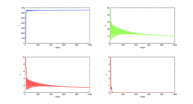
01subscript01\mathcal{R}_{0}\leq 1 iff β0.009513986𝛽0.009513986\beta\leq 0.009513986. We set β=0.003𝛽0.003\beta=0.003 . By theorem (2) i), we have the single equilibrium E0=(666.6666,0,0,0)subscript𝐸0666.6666000E_{0}=(666.6666,0,0,0) which is globally asymptotically stable by theorem (3).

Using a constant history function S=(25,50,10,5)𝑆2550105S=(25,50,10,5) for t(0,10)𝑡010t\in(0,10) and DDE 23 tool from Matlab, we obtain the figure (1).

Example 2.

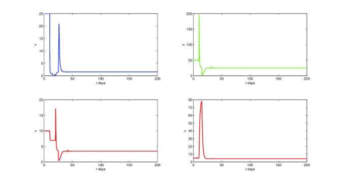
Now, set β=0.0096𝛽0.0096\beta=0.0096, so R0>1subscript𝑅01R_{0}>1. Computing R1subscript𝑅1R_{1} from its definition we have R1=keα1τ1eα2τ2auf(x^,y^,v^)subscript𝑅1𝑘superscript𝑒subscript𝛼1subscript𝜏1superscript𝑒subscript𝛼2subscript𝜏2𝑎𝑢𝑓^𝑥^𝑦^𝑣R_{1}=\frac{ke^{-\alpha_{1}\tau_{1}}e^{-\alpha_{2}\tau_{2}}}{au}f(\hat{x},\hat{y},\hat{v}), where

y^=bc,v^=y^keα2τ2u,n(x^)f(x^,y^,v^)v^=0,formulae-sequence^𝑦𝑏𝑐formulae-sequence^𝑣^𝑦𝑘superscript𝑒subscript𝛼2subscript𝜏2𝑢𝑛^𝑥𝑓^𝑥^𝑦^𝑣^𝑣0\hat{y}=\frac{b}{c},\quad\hat{v}=\frac{\hat{y}ke^{-\alpha_{2}\tau_{2}}}{u},\quad n(\hat{x})-f(\hat{x},\hat{y},\hat{v})\hat{v}=0,

therefore R1=0.97091<1subscript𝑅10.970911R_{1}=0.97091<1 and we have then, a second equilibrium

E1=(659.461141,5.962025,0.826548,0).subscript𝐸1659.4611415.9620250.8265480E_{1}=(659.461141,5.962025,0.826548,0).

Using the history function from previous example we can plot the solution with Matlab. By theorem (4), E1subscript𝐸1E_{1} is globally asymptotically stable as we can see in figure (2).

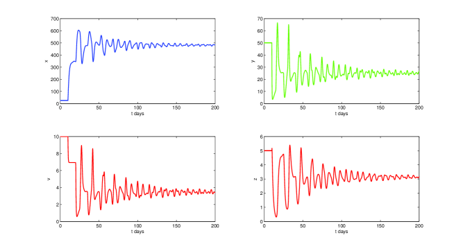
Finally, for β=1𝛽1\beta=1, we have R0>1subscript𝑅01R_{0}>1 and R1=6.088529subscript𝑅16.088529R_{1}=6.088529, so there exists an infection free equilibrium E0subscript𝐸0E_{0} and two equilibria

E1=(1.461792,152.184859,21.098236,0),subscript𝐸11.461792152.18485921.0982360E_{1}=(1.461792,152.184859,21.098236,0),

and

E2=(1.537198,25,3.465889,4.070823).subscript𝐸21.537198253.4658894.070823E_{2}=(1.537198,25,3.465889,4.070823).

By theorem (5) we have global stability of equilibrium E2subscript𝐸2E_{2}. The solutions are showed in figure (3).

Example 3.

In order to show that our model, generalizes the previous articles, we propose the following incidence function to show our results:

f(x,y,v)=βx(1+αy)(1+γv),𝑓𝑥𝑦𝑣𝛽𝑥1𝛼𝑦1𝛾𝑣f(x,y,v)=\frac{\beta x}{(1+\alpha y)(1+\gamma v)},

this function satisfies

  • i)

    f(0,y,v)=0,y,v0formulae-sequence𝑓0𝑦𝑣0for-all𝑦𝑣0f(0,y,v)=0,\quad\forall y,v\geq 0.

  • ii)

    fx=β(1+αy)(1+γv)>0,x,y,v>0formulae-sequence𝑓𝑥𝛽1𝛼𝑦1𝛾𝑣0for-all𝑥𝑦𝑣0\frac{\partial f}{\partial x}=\frac{\beta}{(1+\alpha y)(1+\gamma v)}>0,\quad\forall x,y,v>0.

  • iii a)

    fy=βxα(αy+1)2(γv+1)0x,y,v0formulae-sequence𝑓𝑦𝛽𝑥𝛼superscript𝛼𝑦12𝛾𝑣10for-all𝑥𝑦𝑣0\frac{\partial f}{\partial y}=-{\frac{\beta\,x\alpha}{\left(\alpha y+1\right)^{2}\left(\gamma v+1\right)}}\leq 0\quad\forall x,y,v\geq 0.

  • iii b)

    fv=βxγ(αy+1)(γv+1)20,x,y,v0.formulae-sequence𝑓𝑣𝛽𝑥𝛾𝛼𝑦1superscript𝛾𝑣120for-all𝑥𝑦𝑣0\frac{\partial f}{\partial v}=-{\frac{\beta\,x\gamma}{\left(\alpha y+1\right)\left(\gamma v+1\right)^{2}}}\leq 0,\quad\forall x,y,v\geq 0.

Set the other functions and parameters as in example 1, then we obtain model:

x˙˙𝑥\displaystyle\dot{x} =λdx+rx(1xK)βxv(1+y)(1+v),absent𝜆𝑑𝑥𝑟𝑥1𝑥𝐾𝛽𝑥𝑣1𝑦1𝑣\displaystyle=\lambda-dx+rx\left(1-\frac{x}{K}\right)-\frac{\beta xv}{(1+y)(1+v)},
y˙˙𝑦\displaystyle\dot{y} =βx(tτ1)v(tτ1)(1+y(tτ1))(1+v(tτ1))eα1τ1aypyz,absent𝛽𝑥𝑡subscript𝜏1𝑣𝑡subscript𝜏11𝑦𝑡subscript𝜏11𝑣𝑡subscript𝜏1superscript𝑒subscript𝛼1subscript𝜏1𝑎𝑦𝑝𝑦𝑧\displaystyle=\frac{\beta x(t-\tau_{1})v(t-\tau_{1})}{(1+y(t-\tau_{1}))(1+v(t-\tau_{1}))}e^{-\alpha_{1}\tau_{1}}-ay-pyz,
v˙˙𝑣\displaystyle\dot{v} =keα2τ2y(tτ2)uv,absent𝑘superscript𝑒subscript𝛼2subscript𝜏2𝑦𝑡subscript𝜏2𝑢𝑣\displaystyle=ke^{-\alpha_{2}\tau_{2}}y(t-\tau_{2})-uv,
z˙˙𝑧\displaystyle\dot{z} =cyzbz,absent𝑐𝑦𝑧𝑏𝑧\displaystyle=cyz-bz,

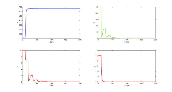
The infection free equilibrium is E0=(666.6666,0,0,0)subscript𝐸0666.6666000E_{0}=(666.6666,0,0,0) as in previous cases, with R0=70.0722745βsubscript𝑅070.0722745𝛽R_{0}=70.0722745\beta, so R0>1subscript𝑅01R_{0}>1 iff β>0.01427097𝛽0.01427097\beta>0.01427097. Therefore, if we set β=0.1𝛽0.1\beta=0.1 then we have R0>1subscript𝑅01R_{0}>1, R1=4.9234560677357286281subscript𝑅14.9234560677357286281R_{1}=4.9234560677357286281 and there exists two more equilibria points,

E1=(115.436331,183.268932,25.407594,0),E2=(481.791432,25,3.465889,3.138764)formulae-sequencesubscript𝐸1115.436331183.26893225.4075940subscript𝐸2481.791432253.4658893.138764E_{1}=(115.436331,183.268932,25.407594,0),\quad E_{2}=(481.791432,25,3.465889,3.138764)

with E2subscript𝐸2E_{2} globally asymptotically stable. The solutions are showed in figure (4).

5 Conclusions

In this paper we studied the global properties of a model of infinitely distributed delayed viral infection, that considers a nonlinear CTL immune response, given by w(y,z)=ϕ1(y)ϕ2(z)𝑤𝑦𝑧subscriptitalic-ϕ1𝑦subscriptitalic-ϕ2𝑧w(y,z)=\phi_{1}(y)\phi_{2}(z) and a general incidence function of the form f(x,y,v)v𝑓𝑥𝑦𝑣𝑣f(x,y,v)v, where w𝑤w and f𝑓f satisfy certain conditions derived from previous works and biological meanings. Even when there exists variety of papers that include the CTL immune response (see for example [1, 3, 4, 5, 7]) and general incidence functions of various types (see [5, 7, 9] ), the model proposed in this article includes a family of the works studied by several authors, and their conclusions can be seen as a particular case of our theorems. There lies its importance and relevance.

The model presents always an infection free positive equilibrium E0=(x¯,0,0,0)subscript𝐸0¯𝑥000E_{0}=(\bar{x},0,0,0), and two types of chronic infection equilibria: the CTL inactivated infection equilibrium (CTL-IE) E1=(x1,y1,v1,0)subscript𝐸1subscript𝑥1subscript𝑦1subscript𝑣10E_{1}=(x_{1},y_{1},v_{1},0) and the CTL activated infection equilibrium (CTL-AE) E2=(x2,y2,v2,z2)subscript𝐸2subscript𝑥2subscript𝑦2subscript𝑣2subscript𝑧2E_{2}=(x_{2},y_{2},v_{2},z_{2}). The coexistence of these equilibria is determined by the basic reproduction number R0subscript𝑅0R_{0} and the viral reproduction number R1subscript𝑅1R_{1}, those were defined in section 2 and are given in terms of parameters and the functions f(x,y,v),fi(τ),ϕ1(y)𝑓𝑥𝑦𝑣subscript𝑓𝑖𝜏subscriptitalic-ϕ1𝑦f(x,y,v),f_{i}(\tau),\phi_{1}(y) and ϕ2(z)subscriptitalic-ϕ2𝑧\phi_{2}(z). The results show that R0>R1subscript𝑅0subscript𝑅1R_{0}>R_{1} and the system admits always a positive infection free equilibrium E0subscript𝐸0E_{0}, which is the unique equilibrium when R01subscript𝑅01R_{0}\leq 1. If R0>1subscript𝑅01R_{0}>1 then, in addition to E0subscript𝐸0E_{0} we have only the CTL-IE (when R11subscript𝑅11R_{1}\leq 1), or the coexistence of the CTL-IE and CTL-AE (R1>1subscript𝑅11R_{1}>1).

We proved, by construction of a Lyapunov function, that whenever the equilibrium E0subscript𝐸0E_{0} is unique (R01subscript𝑅01R_{0}\leq 1) and R01subscript𝑅01R_{0}\neq 1, E0subscript𝐸0E_{0} is globally asymptotically stable, moreover when R0>1subscript𝑅01R_{0}>1 and R1<1subscript𝑅11R_{1}<1 the CTL-IE, E1subscript𝐸1E_{1} is globally asymptotically stable. In the case of CTL-AE, E2subscript𝐸2E_{2} we obtained conditions for global stability only in the case f3(τ)=δ(τ)subscript𝑓3𝜏𝛿𝜏f_{3}(\tau)=\delta(\tau), ie, when the equation of z˙˙𝑧\dot{z} does not present delay. The results indicate that in this case, the equilibrium E2subscript𝐸2E_{2} is globally asymptotically stable when R1>1subscript𝑅11R_{1}>1 and conditions i)H4i)-H_{4} hold. It will be of interest to find conditions that guarantee the global stability of the E2subscript𝐸2E_{2} with a general f3(τ)subscript𝑓3𝜏f_{3}(\tau), this topic can be taken as a future work.
Acknowledgments

This article was supported in part by Mexican SNI under grant 15284 and CONACYT Scholarship 295308.

6 Figures

Refer to caption
Figure 1: Global stability of infection free equilibrium for 0<1subscript01\mathcal{R}_{0}<1.
Refer to caption
Figure 2: Global stability of CTL-IE E1subscript𝐸1E_{1} for 0>1>R1subscript01subscript𝑅1\mathcal{R}_{0}>1>R_{1}.
Refer to caption
Figure 3: Global stability of CTL-AE E2subscript𝐸2E_{2} for R0>1,R1>1formulae-sequencesubscript𝑅01subscript𝑅11R_{0}>1,R_{1}>1.
Refer to caption
Figure 4: Global stability of CTL-AE E2subscript𝐸2E_{2} for f(x,y,v)=βx(1+αy)(1+γv)𝑓𝑥𝑦𝑣𝛽𝑥1𝛼𝑦1𝛾𝑣f(x,y,v)=\frac{\beta x}{(1+\alpha y)(1+\gamma v)}, with R0>1,R1>1formulae-sequencesubscript𝑅01subscript𝑅11R_{0}>1,R_{1}>1.

References

References

  • [1] Nowak M. A. and Bangham C. R. Population dynamics of immune responses to persistent viruses. Science, 272(5258):74, 1996.
  • [2] Xu S. Global stability of the virus dynamics model with Crowley-Martin functional response. Electronic Journal of Qualitative Theory of Differential Equations, 9:1–10, 2012.
  • [3] Li X. and Fu S. Global stability of a virus dynamics model with intracellular delay and CTL immune response. Mathematical Methods in the Applied Sciences, 38(3):420–430, 2015.
  • [4] Yang Y. Stability and hopf bifurcation of a delayed virus infection model with Beddington–DeAngelis infection function and cytotoxic T-lymphocyte immune response. Mathematical Methods in the Applied Sciences, 38(18):5253–5263, 2015.
  • [5] Yang H. and Wei J. Analyzing global stability of a viral model with general incidence rate and cytotoxic T lymphocytes immune response. Nonlinear Dynamics, 82(1-2):713–722, 2015.
  • [6] Hattaf K., Yousfi N., and Tridane A. Mathematical analysis of a virus dynamics model with general incidence rate and cure rate. Nonlinear Analysis: Real World Applications, 13(4):1866–1872, 2012.
  • [7] Hattaf K., Yousfi N., and Tridane A. Global stability analysis of a generalized virus dynamics model with the immune response. Canadian Applied Mathematics Quarterly, 20(4):499–518, 2012.
  • [8] Wang X., Tao Y., and Song X. Global stability of a virus dynamics model with Beddington–DeAngelis incidence rate and CTL immune response. Nonlinear Dynamics, 66(4):825–830, 2011.
  • [9] Shu H., Wang L., and Watmough J. Global stability of a nonlinear viral infection model with infinitely distributed intracellular delays and CTL immune responses. SIAM Journal on Applied Mathematics, 73(3):1280–1302, 2013.
  • [10] Ji Y. and Liu L. Global stability of a delayed viral infection model with nonlinear immune response and general incidence rate. Discrete & Continuous Dynamical Systems-Series B, 21(1), 2016.
  • [11] Wang J., Guo M., Liu X., and Zhao Z. Threshold dynamics of HIV–1 virus model with cell-to-cell transmission, cell-mediated immune responses and distributed delay. Applied Mathematics and Computation, 291:149–161, 2016.
  • [12] FV A. and Haddock J. On determining phase spaces for functional differential equations. Funkcialaj Ekvacioj, 31:331–347, 1988.