Particle-without-Particle: a practical pseudospectral collocation method for linear partial differential equations with distributional sources

Abstract

Partial differential equations with distributional sources—in particular, involving (derivatives of) delta distributions—have become increasingly ubiquitous in numerous areas of physics and applied mathematics. It is often of considerable interest to obtain numerical solutions for such equations, but any singular (“particle”-like) source modeling invariably introduces nontrivial computational obstacles. A common method to circumvent these is through some form of delta function approximation procedure on the computational grid; however, this often carries significant limitations on the efficiency of the numerical convergence rates, or sometimes even the resolvability of the problem at all.
In this paper, we present an alternative technique for tackling such equations which avoids the singular behavior entirely: the “Particle-without-Particle” method. Previously introduced in the context of the self-force problem in gravitational physics, the idea is to discretize the computational domain into two (or more) disjoint pseudospectral (Chebyshev-Lobatto) grids such that the “particle” is always at the interface between them; thus, one only needs to solve homogeneous equations in each domain, with the source effectively replaced by jump (boundary) conditions thereon. We prove here that this method yields solutions to any linear PDE the source of which is any linear combination of delta distributions and derivatives thereof supported on a one-dimensional subspace of the problem domain. We then implement it to numerically solve a variety of relevant PDEs: hyperbolic (with applications to neuroscience and acoustics), parabolic (with applications to finance), and elliptic. We generically obtain improved convergence rates relative to typical past implementations relying on delta function approximations.

1 Introduction

Mathematical models often have to resort—be it out of expediency or mere ignorance—to deliberately idealized descriptions of their contents. A common idealization across different fields of applied mathematics is the use of the Dirac delta distribution, often simply referred to as the delta “function”, for the purpose of describing highly localized phenomena: that is to say, phenomena the length scale of which is significantly smaller, in some suitable sense, than that of the problem into which they figure, and the (possibly complicated) internal structure of which can thus be safely (or safely enough) ignored in favour of a simple “point-like” cartoon. Canonical examples of this from physics are notions such as “point masses” in gravitation or “point charges” in electromagnetism.

Yet, despite their potentially powerful conceptual simplifications, introducing distributions into any mathematical model is something that must be handled with great technical care. In particular, let us suppose that our problem of interest has the very general form

$$\mathcal{L}u=S\quad\mbox{in}\enskip\mathscr{U}\subseteq\mathbb{R}^{n}\,,$$ (1)

where $\mathcal{L}$ is an $n$-dimensional (partial, if $n>1$) differential operator (of arbitrary order $m$), $u$ is a quantity to be solved for (a function, a tensor etc.) and we assume that $S$—the “source”—is distributional in nature, i.e. we have $S:\mathcal{D}(\mathscr{U})\rightarrow\mathbb{R}$, where we use the common notation $\mathcal{D}(\mathscr{U})$ to refer to the set of smooth compactly-supported functions, i.e. “test functions”, on $\mathscr{U}$. It follows, therefore, that $u$—if it exists—must also be distributional in nature. So strictly speaking, from the point of view of the classic theory of distributions schwartz_theorie_1957 , the problem (1) is only well-defined—and hence may admit distributional solutions $u$—provided that $\mathcal{L}$ is linear.

The problem with a nonlinear $\mathcal{L}$ is essentially that, classically, products of distributions do not make sense schwartz_sur_1954 . While there has certainly been work by mathematicians aiming to generalize the theory of distributions so as to accommodate this possibility li_review_2007 ; colombeau_nonlinear_2013 ; bottazzi_grid_2017 , in the standard setting we are only really allowed to talk of linear problems of the form (1). Opportunely, very many of the typical problems in physics and applied mathematics involving distributions take precisely this form.

The inspiration for considering (1) in general in this paper actually comes from a setting where one does, in fact, encounter non-linearities a priori: namely, gravitational physics. (For a general discussion regarding the treatment of distributions therein, see Ref. geroch_strings_1987 .) In particular, equations such as (1) arise when attempting to describe the backreaction of a body with a “small” mass upon the spacetime through which it moves—known as its self-force mino_gravitational_1997 ; quinn_axiomatic_1997 ; detweiler_self-force_2003 ; gralla_rigorous_2008 ; gralla_note_2011 ; poisson_motion_2011 ; blanchet_mass_2011 ; spallicci_self-force_2014 ; pound_motion_2015 ; wardell_self-force:_2015 . (A similar version of this problem exists in electromagnetism, where a “small” charge backreacts upon the electromagnetic field that determines its motion dirac_classical_1938 ; dewitt_radiation_1960 ; barut_electrodynamics_1980 ; poisson_motion_2011 .) In the full Einstein equations of general relativity, which can be regarded as having the schematic form (1) with $u$ describing the gravitational field (that is, the spacetime geometry, in the form of the metric) and $S$ denoting the matter source (the stress-energy-momentum tensor), $\mathcal{L}$ is a nonlinear operator. Nevertheless, for a distributional $S$ (representing the “small” mass as a “point particle” source) one can legitimately seek solutions to a linearized version of (1) in the context of perturbation theory, i.e. at first order in an expansion of $\mathcal{L}$ in the mass. The detailed problem, in this case, turns out to be highly complex, and in practice, $u$ must be computed numerically. The motivation for this, we may add, is not just out of purely theoretical or foundational concern—the calculation of the self-force is also of significant applicational value for gravitational wave astronomy. To wit, it will in fact be indispensable for generating accurate enough waveform templates for future space-based gravitational wave detectors such as LISA amaro-seoane_et_al._gravitational_2013 ; amaro-seoane_et_al._laser_2017 vis-à-vis extreme-mass-ratio binary systems, which are expected to be among the most fruitful sources thereof. For these reasons, having at our disposal a practical and efficient numerical method for handling equations of the form (1) is of consequential interest.

What is more, these sorts of partial differential equations (PDEs) arise frequently in other fields as well; indeed, (1) can adequately characterize quite a wide variety of (linear) mathematical phenomena assumed to be driven by “localized sources”. A few examples, which we will consider one by one in different sections of this paper, are the following:

1. First-order hyperbolic PDEs: in neuroscience, advection-type PDEs with a delta function source can be used in the modeling of neural populations haskell_population_2001 ; casti_population_2002 ; caceres_analysis_2011 ; caceres_blow-up_2016 ;

2. Parabolic PDEs: in finance, heat-type PDEs with delta function sources are sometimes used to model price formation lasry_mean_2007 ; markowich_parabolic_2009 ; caffarelli_price_2011 ; burger_boltzmann-type_2013 ; achdou_partial_2014 ; pietschmann_partial_2012 ;

3. Second-order hyperbolic PDEs: in acoustics, wave-type PDEs with delta function (or delta derivative) sources are used to model monopoles (or, respectively, multipoles) petersson_stable_2010 ; kaltenbacher_computational_2017 ; more complicated equations of this form also appear, for example, in seismology models romanowicz_seismology_2007 ; aki_quantitative_2009 ; shearer_introduction_2009 ; madariaga_seismic_2007 ; petersson_stable_2010 , which we will briefly comment upon.

4. Elliptic PDEs: Finally, we will look at a simple Poisson equation with a singular source tornberg_numerical_2004 ; such equations can describe, for example, the potential produced by a very localized charge in electrostatics.

1.1 Scope of this paper

The purpose of this paper is to explicate and generalize a practical method for numerically solving equations like (1), as well as to illustrate its broad applicability to the various problems listed in (i)-(iv) above. Previously implemented with success only in the specific context of the self-force problem canizares_extreme-mass-ratio_2011 ; canizares_efficient_2009 ; canizares_pseudospectral_2010 ; canizares_time-domain_2011 ; canizares_tuning_2011 ; jaramillo_are_2011 ; canizares_overcoming_2014 ; oltean_frequency-domain_2017 , we dub it the “Particle-without-Particle” (PwP) method. (Other methods for the computation of the self-force have also been developed based on matching the properties of the solutions on the sides of the delta distributions—see, e.g., the indirect (source-free) integration method of Refs. aoudia_source-free_2011 ; ritter_fourth-order_2011 ; spallicci_towards_2012 ; spallicci_fully_2014 ; ritter_indirect_2015 ; ritter_indirect_2015-1 .) The basic idea of the PwP approach is the following: One begins by writing $u$ as a sum of distributions each of which has support outside (plus, if necessary, at the location of) the points where $S$ is supported; one then solves the equations for each of these pieces of $u$ and finally matches them in such a way that their sum satisfies the original problem (1). In fact, as we shall soon elaborate upon, this approach will not work in general for all possible problems of the form (1). However, we will prove that it will always work if, rather than the source being a distribution defined on all of $\mathscr{U}$, we have instead $S:\mathcal{D}(\mathscr{I})\rightarrow\mathbb{R}$ with $\mathscr{I}\subseteq\mathbb{R}$ representing a one-dimensional subspace of $\mathscr{U}$.

To make things more concrete, let us briefly describe this procedure using the simplest possible example: let $f:\mathscr{U}\rightarrow\mathbb{R}$ be an arbitrary given function and suppose $S=f\delta$ where $\delta:\mathcal{D}(\mathscr{I})\rightarrow\mathbb{R}$ is the delta function supported at some point $x_{p}\in\mathscr{I}$. Then, to solve (1), one would assume the decomposition (or “ansatz”) $u=u^{-}\Theta^{-}+u^{+}\Theta^{+}$ with $\Theta^{\pm}:\mathcal{D}(\mathscr{I})\rightarrow\mathbb{R}$ denoting appropriately defined Heaviside distributions (supported to the right/left of $x_{p}$, respectively), and $u^{\pm}:\mathscr{U}\rightarrow\mathbb{R}$ being simple functions (not distributions) to be solved for. Inserting such a decomposition for $u$ into (1), one obtains homogeneous equations $\mathcal{L}u^{\pm}=0$ on the appropriate domains, supplemented by the necessary boundary conditions (BCs) for these equations at $x_{p}\in\mathscr{I}$, explicitly determined by $f$. Generically, the latter arise in the form of relations between the limits of $u^{-}$ and $u^{+}$ (and/or the derivatives thereof) at $x_{p}$, and for this reason are called “jump conditions” (JCs). Effectively, the latter completely replace the “point” source $S$ in the original problem, now simply reduced to solving sourceless equations—hence the nomenclature of the method.

While in principle one can certainly contemplate the adaptation of these ideas into a variety of established approaches for the numerical solution of PDEs, we will focus specifically on their implementation through pseudospectral collocation (PSC) methods on Chebyshev-Lobatto (CL) grids. The principal advantages thereof lie in their typically very efficient (exponential) rates of numerical convergence as well as the ease of incorporating and modifying BCs (JCs) throughout the evolution. Indeed, PSC methods have enjoyed very good success in past work canizares_extreme-mass-ratio_2011 ; canizares_efficient_2009 ; canizares_pseudospectral_2010 ; canizares_time-domain_2011 ; canizares_tuning_2011 ; jaramillo_are_2011 ; canizares_overcoming_2014 ; oltean_frequency-domain_2017 on the PwP approach for self-force calculations (and in gravitational physics more generally grandclement_spectral_2009 , including arbitrary precision implementations santos-olivan_pseudo-spectral_2018 ), and so we shall not deviate very much from this recipe in the models considered in this paper. Essentially the main difference will be that here, instead of the method of lines which featured in most of the past PwP self-force work, we will for the most part carry out the time evolution using the simplest first-order forward finite difference scheme; we do this, on the one hand, so that we may illustrate the principle of the method explicitly in a very elementary way without too many technical complications, and on the other, to show how well it can work even with such basic tactics. Depending on the level of accuracy and computational efficiency required for any realistic application, these procedures can naturally be complexified (to higher order, more domains, more complicated domain compactifications etc.) for properly dealing with the sophistication of the problem at hand.

To summarize, past work using the PwP method only solved a specific form of Eq. (1) pertinent to the self-force problem: that is, with a particular choice of $\mathcal{L}$ and $S$ (upon which we will comment more later). It did not consider the question of the extent to which the idea of the method could be useful in general for solving distributionally-sourced PDEs. These appear, as enumerated above, in many other fields of study—and we submit that a method such as this would be of valuable benefit to researchers working therein. The novelty of the present paper will thus be to formulate a completely general PwP method for any distributionally-sourced (linear) problem of the form (1) with the single limiting condition that ${\rm supp}(S)\subset\mathscr{I}\subseteq\mathscr{U}$ where ${\rm dim}(\mathscr{I})=1$. We will prove rigorously why and how the method works for such problems, and then we will implement it to obtain numerical solutions to the variety of different applications mentioned earlier in order to illustrate its broad practicability. We will see that, in general, this method either matches or improves upon the results of other methods existent in the literature for tackling distributionally-sourced PDEs—and we turn to a more detailed discussion of this topic in the next subsection.

1.2 Comparison with other methods in the literature

Across all areas of application, the most commonly encountered—and, perhaps, most naively suggestible—strategy for numerically solving equations of the form (1) is to rely upon some sort of delta function approximation procedure on the computational grid tornberg_numerical_2004 ; jung_collocation_2009 ; jung_note_2009 ; petersson_discretizing_2016 . For instance, the simplest imaginable choice in this vein is just a narrow hat function (centered at the point where the delta function is supported, and having total measure $1$) which, for better accuracy, one can upgrade to higher-order polynomials, or even trigonometric functions. Another readily evocable possibility is to use a narrow Gaussian—and indeed, this is one option that has in fact been tried in self-force computations as well (see Ref. lopez-aleman_perturbative_2003 , for example). However, this unavoidably introduces into the problem an additional, artificial length scale: that is, the width of the Gaussian, which a priori need not have anything to do with the actual (“physical”) length scale of the source. Moreover, there is the evident drawback that no matter how small this artificial length scale is chosen, the solutions will never be well-resolved close to the distributional source location: there will always be some sort of Gibbs-type phenomenon there.

Methods for solving (1) which are closer in spirit to our PwP method have been explored in Refs. field_discontinuous_2009 and shin_spectral_2011 . In particular, both of these works have used the idea of placing the distributional source at the interface of computational grids—however, they tackle the numerical implementation differently than we do.

In the case of Ref. field_discontinuous_2009 —which, incidentally, is also concerned with the self-force problem—the difference is that the authors use a discontinuous Galerkin method (rather than spectral methods, as in our PwP approach), and the effect of the distributional source is accounted for via a modification of the numerical flux at the “particle” location. This relies essentially upon a weak formulation of the problem, wherein a choice has to be made about how to assign measures to the distributional terms over the relevant computational domains. In contrast, we directly solve only for smooth solutions supported away from the “particle” location, and account for the distributional source simply by imposing adequate boundary—i.e. jump— conditions there.

Ref. shin_spectral_2011 is closer to our approach in this sense, as the authors there also use spectral methods and also account for the distributional source via jump conditions. However, the difference with our method is that Ref. shin_spectral_2011 treats these jump conditions as additional constraints (rather than built-in boundary conditions) for the smooth solutions away from the distributional source, thus over-determining the problem. That being the case, the authors are led to the need to define a functional (expressing how well the differential equations plus the jump conditions are satisfied) to be minimized—constituting what they refer to as a “least squares spectral collocation method”. There is however no unique way to choose this functional. Moreover, the complication of introducing it is not at all necessary: our approach, in contrast, simply replaces the discretization of (the homogeneous version of) the differential equations at the “particle” location with the corresponding jump conditions (i.e. it imposes the jump conditions as boundary conditions, by construction—something which PSC methods are precisely designed to be able to handle), leading to completely determined systems in all cases which are solved directly, without further complications.

Finally, neither Ref. field_discontinuous_2009 nor shin_spectral_2011 analyzed to any significant extent the conditions under which their methods might be applicable to more general distributionally-sourced PDEs. As mentioned, in the present paper we will devote a careful proof entirely to this issue.

This paper is structured as follows. Following some mathematical preliminaries in Section 2, we prove in Section 3 how the PwP method can be formulated and applied to problems with the most general possible “point” source $S:\mathcal{D}(\mathscr{I})\rightarrow\mathbb{R}$, that is, one containing an arbitrary number of (linearly combined) delta derivatives and supported at an arbitrary number of points in $\mathscr{I}$. Thus, one can use it on any type of (linear) PDE involving such sources, which we illustrate with the applications listed in (i)-(iv) above in Sections 4-7 respectively. Finally, we give concluding remarks in Section 8.

2 Setup

We wish to begin by establishing some basic notation and then reviewing some pertinent properties of distributions that we will need to make use of later on. While we will certainly strive to maintain a fair level of mathematical rigour here and throughout this paper (at least, insofar as a certain amount of formal precaution is inevitably necessary when dealing with distributions), our principal aim remains that of presenting practical methodologies; hence the word “distribution” may at times be liberally interchanged for “function” (e.g. we may say “delta function” instead of “delta distribution”) and some notation possibly slightly abused, when the context is clear enough to not pose dangers for confusion.

2.1 Distributionally-sourced linear PDEs

Consider the problem (1) with $S:\mathcal{D}(\mathscr{I})\rightarrow\mathbb{R}$, where $\mathscr{I}\subseteq\mathbb{R}$ is a one-dimensional subspace of $\mathscr{U}\subseteq\mathbb{R}^{n}$, as discussed in the introduction. Then we can view $\mathscr{U}$ as a product space, $\mathscr{U}=\mathscr{I}\times\mathscr{V}$ with $\mathscr{V}=\mathscr{U}/\mathscr{I}\subseteq\mathbb{R}^{n-1}$, and write coordinates on $\mathscr{U}$ as $\mathbf{x}=(x,\mathbf{y})$ with $x\in\mathscr{I}$ and $\mathbf{y}=(y_{1},\ldots,y_{n-1})\in\mathscr{V}$, such that

$$f:\mathscr{U}=\mathscr{I}\times\mathscr{V}\subseteq\mathbb{R}\times\mathbb{R}^{n-1}=\mathbb{R}^{n} \rightarrow\mathbb{R}$$

$$\mathbf{x}\,\,=\,\,\left(x,\mathbf{y}\right)\,=\,\left(x,y_{1},\ldots,y_{n-1}\right) \mapsto f\left(\mathbf{x}\right)$$ (2)

denotes any arbitrary function on $\mathscr{U}$.

It is certainly possible, in the setup we are about to describe, to have $\mathscr{V}=\emptyset$, i.e. problems involving just ODEs (on $\mathscr{U}=\mathscr{I}$) of the form (1)—and, in fact, our first elementary example illustrating the PwP method in the following section will be of such a kind. For the more involved numerical examples we will study in later sections, we will most often be dealing with functions of two variables, $x\in\mathscr{I}$ for “space” (or some other pertinent parameter) and $t\in\mathscr{V}\subseteq\mathbb{R}$ for time.

For any function (2) involved in these problems, we will sometimes use the notation $f^{\prime}=\partial_{x}f$ for the “spatial” derivative; also, we may employ $\dot{f}=\partial_{t}f$ for the partial derivative with respect to time $t$ when $\{t\}$ is (a subspace of) $\mathscr{V}$.

Now, as in the introduction, let $\mathcal{L}$ be any general $m$-th order linear differential operator. The sorts of PDEs (1) that we will be concerned with have the basic form

$$\mathcal{L}u=S=f\delta_{\left(p\right)}+g\delta_{\left(p\right)}^{{}^{\prime}}+\cdots\,,$$ (3)

where $f(\mathbf{x})$, $g(\mathbf{x})$ etc. are “source” functions prescribed by the problem at hand, and we employ the convenient notation

$$\delta_{\left(p\right)}\left(x\right)=\delta\left(x-x_{p}\left(\mathbf{y}\right)\right)$$ (4)

to indicate the Dirac delta distribution on $\mathscr{I}$ centered at the “particle location” $x_{p}(\mathbf{y})$—the functional form of which can be either specified a priori, or determined via some given prescription as the solution $u$ itself is evolved. When there is no risk of confusion, we may sometimes omit the $\mathbf{y}$ dependence in our notation and simply write $x_{p}$.

In fact, our PwP method can even deal with multiple, say $M$, “particles”. PwP computations of the self-force have actually only required $M=1$ (there being only one “particle” involved in the problem), so the general $M\geq 1$ case has not been considered up to now. Concordantly, to express our problem of interest (3) in the most general possible form, let us employ the typical PDE notation for “multi-indices” evans_partial_1998 , $\alpha=(\alpha_{0},\alpha_{1},\ldots,\alpha_{n-1})$ with each $\alpha_{I}\in\mathbb{Z}^{\geq}$ being a non-negative integer (indexed from $I=0$ to $I=n-1$ so as to make sense vis-à-vis our coordinate notation on $\mathscr{U}$, instead of the more usual practice to label them from $1$ to $n$), and $|\alpha|=\sum_{I=0}^{n-1}\alpha_{I}$. Furthermore, we define $\alpha!=\prod_{I=0}^{n-1}\alpha_{I}!$. Thus, the most general $m$-th order linear partial differential operator can be written as $\mathcal{L}=\sum_{|\alpha|\leq m}\xi^{\alpha}(\mathbf{x})D^{\alpha}$ where $\xi^{\alpha}:\mathscr{U}\rightarrow\mathbb{R}$ are arbitrary functions and $D^{\alpha}=\partial^{|\alpha|}/\partial x^{\alpha_{0}}\partial y_{1}^{\alpha_{1}}\cdots\partial y_{n-1}^{\alpha_{n-1}}$. Hence, we are dealing with any problem which can be placed into the form

$$\sum_{|\alpha|\leq m}\xi^{\alpha}\left(\mathbf{x}\right)D^{\alpha}u\left(\mathbf{x}\right)=\sum_{i=1}^{M}\sum_{j=0}^{K}f^{ij}\left(\mathbf{x}\right)\delta^{(j)}\left(x-x_{p_{i}}\left(\mathbf{y}\right)\right)\,,$$ (5)

with $f^{ij}:\mathscr{U}\rightarrow\mathbb{R}$ denoting the “source” functions (for the $j$-th delta derivative of the $i$-th particle) and $K\in\mathbb{Z}^{\geq}$ the highest order of the delta function derivatives in $S$, appropriately supplemented by initial/boundary conditions (ICs/BCs).

Let us give a few basic examples to render this setup more palpable. One very simple example—that which will serve as our first illustration of the PwP method in the next section—is the simple harmonic oscillator with a constant delta function forcing (source) term—that is, the ODE (with $\mathscr{V}=\emptyset$):

$$u^{\prime\prime}+u=a\delta_{\left(p\right)}\,,$$ (6)

where $\delta_{\left(p\right)}(x)=\delta(x-x_{p})$ for some fixed $x_{p}\in\mathscr{I}$, and $a\in\mathbb{R}$. Another example is the wave equation with a moving singular source,

$$\left(\partial_{t}^{2}-\partial_{x}^{2}\right)u\left(x,t\right)=f\left(x,t\right)\delta\left(x-x_{p}\left(t\right)\right)\,,$$ (7)

with $x_{p}(t)$ specified as a function of time.

2.2 Properties of distributions

We now wish to remind the reader of a few basic properties of distributions before proceeding to describe the PwP procedure; for a good detailed exposition, see e.g. Ref. stakgold_greens_2011 .

Let $f:\mathscr{U}\rightarrow\mathbb{R}$ be, as before, any function involved in the problem (5). We denote by

$$f_{p}:\mathscr{V}\rightarrow\, \mathbb{R}$$

$$\mathbf{y}\mapsto\, f_{p}\left({\bf y}\right)=f\left(x_{p}\left({\bf y}\right),{\bf y}\right)$$ (8)

the function evaluated at the “particle” position.

Furthermore, let $\phi\in\mathcal{D}(\mathscr{I})$ be any test function on $\mathscr{I}$. Then we define the action of the distribution associated with $f$ as:

$$\left\langle f,\phi\right\rangle=\int_{\mathscr{I}}{\rm d}x\,f\left(x,\mathbf{y}\right)\phi\left(x\right)\,.$$ (9)

We say that two functions $f$ and $g$ are equivalent in the sense of distributions if

$$\langle f,\phi\rangle=\langle g,\phi\rangle\Leftrightarrow f\equiv g\,.$$ (10)

An identity which will be important for us in discussing the PwP method is the following cortizo_diracs_1995 ; li_review_2007 :

$$f\left(x,\mathbf{y}\right)\delta_{\left(p\right)}^{\left(n\right)}\left(x\right)\equiv\left(-1\right)^{n}\sum_{j=0}^{n}\left(-1\right)^{j}\binom{n}{j}f_{p}^{\left(n-j\right)}\left(\mathbf{y}\right)\delta_{\left(p\right)}^{\left(j\right)}\left(x\right)\,,$$ (11)

where $\delta_{\left(p\right)}^{\left(n\right)}=\partial_{x}^{n}\delta_{\left(p\right)}$. For concreteness, let us write down the first three cases explicitly here:

$$f\left(x,\mathbf{y}\right)\delta_{\left(p\right)}\left(x\right)\equiv\, f_{p}\left(\mathbf{y}\right)\delta_{\left(p\right)}\left(x\right)\,,$$ (12)

$$f\left(x,\mathbf{y}\right)\delta_{\left(p\right)}^{\prime}\left(x\right)\equiv\, -f_{p}^{\prime}\left(\mathbf{y}\right)\delta_{\left(p\right)}\left(x\right)+f_{p}\left(\mathbf{y}\right)\delta_{\left(p\right)}^{\prime}\left(x\right)\,,$$ (13)

$$f\left(x,\mathbf{y}\right)\delta_{\left(p\right)}^{\prime\prime}\left(x\right)\equiv\, f_{p}^{\prime\prime}\left(\mathbf{y}\right)\delta_{\left(p\right)}\left(x\right)-2f_{p}^{\prime}\left(\mathbf{y}\right)\delta_{\left(p\right)}^{\prime}\left(x\right)+f_{p}\left(\mathbf{y}\right)\delta_{\left(p\right)}^{\prime\prime}\left(x\right)\,.$$ (14)

For the interested reader, we offer in Appendix A a proof by induction of the formula (11), which is instructive for appreciating the subtleties generally involved in manipulating distributions.

Let

$$\Theta_{\left(p\right)}^{\pm}\left(x\right)=\Theta\left(\pm\left(x-x_{p}\left(\mathbf{y}\right)\right)\right)$$ (15)

be the Heaviside function which is supported to the right/left (respectively) of $x_{p}$. Then, we have:

$$\partial_{x}\Theta_{\left(p\right)}^{\pm}=\, \pm\delta_{\left(p\right)}\,,$$ (16)

$$\partial_{y_{j}}\Theta_{\left(p\right)}^{\pm}=\, \mp\left(\partial_{y_{j}}x_{p}\right)\delta_{\left(p\right)}\,,$$ (17)

and so on for higher order partials.

For notational expediency, we may sometimes omit the $(p)$ subscript on the Heaviside functions (and derivatives thereof) when the context is sufficiently clear.

3 The “Particle-without-Particle” method

As discussed heuristically in the introduction, the basic idea of our method for solving (5) is to effectively eliminate the “point”-like source or “particle” from the problem by decomposing the solution $u$ into a series of distributions: specifically, Heaviside functions $\Theta^{i}:\mathcal{D}(\mathscr{I})\rightarrow\mathbb{R}$ supported in each of the $M+1$ disjoint regions of $\mathscr{I}\backslash{\rm supp}(S)$ (i.e. ${\rm supp}(\Theta^{i})\cap{\rm supp}(S)=\emptyset,\forall i$ and ${\rm supp}(\Theta^{i})\cap{\rm supp}(\Theta^{j})=\emptyset,\forall i\neq j$) and, if necessary, delta functions (plus delta derivatives) at ${\rm supp}(S)$:

$$u=\sum_{i=0}^{M}u^{i}\Theta^{i}+\sum_{i=1}^{M}\sum_{j=0}^{K-m}h^{ij}\delta_{\left(p_{i}\right)}^{\left(j\right)}\,,$$ (18)

where $u^{i}:\mathscr{U}\rightarrow\mathbb{R}$ and we need to include the second sum with $h^{ij}:\mathscr{V}\rightarrow\mathbb{R}$ only if $K\geq m$.

We will prove in this section that one can always obtain solutions of the form (18) to the problem (5). In particular, inserting (18) into (5) will always yield homogeneous equations

$$\mathcal{L}u^{i}=0\quad\mbox{in}\,\,\left(\mathscr{I}\backslash{\rm supp}(S)\right)\times\mathscr{V}\,,$$ (19)

along with JCs on (the derivatives of) $u$—and possibly (derivatives of) $h^{ij}$ if applicable. In general, we define the “jump” $[\cdot]_{p}:\mathscr{V}\rightarrow\mathbb{R}$ in the value of any function $f:\mathscr{U}\rightarrow\mathbb{R}$ at $x_{p}({\bf y})$ as

$$\left[f\right]_{p}\left({\bf y}\right)=\lim_{x\rightarrow x_{p}({\bf y})^{+}}f\left(x,{\bf y}\right)-\lim_{x\rightarrow x_{p}({\bf y})^{-}}f\left(x,{\bf y}\right)\,.$$ (20)

Henceforth, for convenience, we will generally omit the ${\bf y}$-dependence and simply write $[f]_{p}$.

First we will work through a simple example in order to offer a more concrete sense of the method, and afterwards we will show in general how (18) solves (5).

3.1 Simple example

We illustrate here the application of our PwP method to a very simple ODE (and single-particle) example. We will consider the problem

$$\mathcal{L}u=u^{\prime\prime}+u=a\delta+b\delta^{{}^{\prime}}\,,\enskip x\in\mathscr{I}=\left[-L,L\right]\,,\enskip u\left(\pm L\right)=0\,,$$ (21)

where $\delta$ is simply the delta function centered at $x_{p}=0$.

We begin by decomposing $u$ as

$$u=u^{-}\Theta^{-}+u^{+}\Theta^{+}\,,$$ (22)

where $\Theta^{\pm}(x)=\Theta(\pm x)$, and we insert this into (21). Using (16), the LHS becomes simply

$$\mathcal{L}u\left(x\right)=\, u^{\prime\prime}\left(x\right)+u\left(x\right)$$ (23)

$$=\, \left\{\mathcal{L}u^{-}\left(x\right)\right\}\Theta^{-}\left(x\right)+\left\{\mathcal{L}u^{+}\left(x\right)\right\}\Theta^{+}\left(x\right)$$

$$+\left\{-2\left(u^{-}\left(x\right)\right)^{\prime}+2\left(u^{+}\left(x\right)\right)^{\prime}\right\}\delta\left(x\right)$$

$$+\left\{-u^{-}\left(x\right)+u^{+}\left(x\right)\right\}\delta^{\prime}\left(x\right)\,.$$ (24)

Now before we can equate this to the distributional terms in the source (RHS), we must apply the identity (11). In particular, we use $f(x)\delta(x)\equiv f_{p}\delta(x)$ and $f(x)\delta^{\prime}(x)\equiv-f_{p}^{\prime}\delta(x)+f_{p}\delta^{\prime}(x)$. Thus, the above becomes

$$\mathcal{L}u\left(x\right)\equiv\, \left\{\mathcal{L}u^{-}\left(x\right)\right\}\Theta^{-}\left(x\right)+\left\{\mathcal{L}u^{+}\left(x\right)\right\}\Theta^{+}\left(x\right)$$

$$+\left\{-2\left(u^{-}\right)^{\prime}_{p}+2\left(u^{+}\right)^{\prime}_{p}\right\}\delta\left(x\right)$$

$$+\left\{\left(u^{-}\right)^{\prime}_{p}-\left(u^{+}\right)^{\prime}_{p}\right\}\delta\left(x\right)+\left\{-u_{p}^{-}+u_{p}^{+}\right\}\delta^{\prime}\left(x\right)$$ (25)

$$=\, \left\{\mathcal{L}u^{-}\left(x\right)\right\}\Theta^{-}\left(x\right)+\left\{\mathcal{L}u^{+}\left(x\right)\right\}\Theta^{+}\left(x\right)+\left[u^{\prime}\right]_{p}\delta\left(x\right)+\left[u\right]_{p}\delta^{\prime}\left(x\right)\,.$$ (26)

Plugging this into the DE (21), we have

$$\left\{\mathcal{L}u^{-}\right\}\Theta^{-}+\left\{\mathcal{L}u^{+}\right\}\Theta^{+}+\left[u^{\prime}\right]_{p}\delta+\left[u\right]_{p}\delta^{\prime}\equiv a\delta+b\delta^{{}^{\prime}}\,.$$ (27)

Therefore the original problem is equivalent to the system of equations:

$$\begin{cases}\mathcal{L}u^{-}=0,&x\in\mathscr{D}^{-}=\left[-L,0\right]\,,\enskip u^{-}\left(-L\right)=0\,,\\ \mathcal{L}u^{+}=0,&x\in\mathscr{D}^{+}=\left[0,L\right]\,,\enskip u^{+}\left(L\right)=0\,,\\ \left[u\right]_{p}=b,&\left[u^{\prime}\right]_{p}=a\,.\end{cases}$$ (28)

Let us solve (28), for simplicity, taking $L=\pi/4$. The left homogeneous equation in (28) has the general solution $u^{-}=A^{-}\cos(x)+B^{-}\sin(x)$, and the BC tells us that $0=u^{-}(-\pi/4)=\frac{1}{\sqrt{2}}(A^{-}-B^{-})$, i.e.

$$A^{-}-B^{-}=0\,.$$ (29)

The right homogeneous equation in (28) similarly has general solution $u^{+}=A^{+}\cos(x)+B^{+}\sin(x)$, with the BC stating $0=u^{+}(\pi/4)=\frac{1}{\sqrt{2}}(A^{+}+B^{+})$, i.e.

$$A^{+}+B^{+}=0\,.$$ (30)

So far we have two equations (29)-(30) for four unknowns (the integration constants in the general solutions). It is the JCs in (28) that provide us with the remaining necessary equations to fix the solution. We have $u^{-}(0)=A^{-}$, $(u^{-})^{\prime}(0)=B^{-}$, $u^{+}(0)=A^{+}$ and $(u^{+})^{\prime}(0)=B^{+}$ (understood in the appropriate limit approaching $x_{p}=0$). Hence the JCs tell us:

$$b=\, \left[u\right]_{p}=u^{+}(0)-u^{-}(0)=A^{+}-A^{-}\,,$$ (31)

$$a=\, \left[u^{\prime}\right]_{p}=(u^{+})^{\prime}(0)-(u^{-})^{\prime}(0)=B^{+}-B^{-}\,.$$ (32)

(We can think of the JCs as a mixing of the degrees of freedom in the homogeneous solutions in such a way that they “link together” to produce the solution generated by the original distributional source.) Solving (29)-(32), we get $A^{-}=-\frac{a+b}{2}=B^{-}$, $A^{+}=-\frac{a-b}{2}=-B^{+}$. We now have the full solution to our original problem (21):

$$u\left(x\right)=-\frac{a+b}{2}\left(\cos\left(x\right)+\sin\left(x\right)\right)\Theta\left(-x\right)-\frac{a-b}{2}\left(\cos\left(x\right)-\sin\left(x\right)\right)\Theta\left(x\right)\,.$$ (33)

3.2 General proof

Suppose we have $M$ “particles” located at ${\rm supp}(S)=\{x_{p_{i}}\}_{i=1}^{M}\subset\mathscr{I}$, as in the problem (5), with $x_{p_{1}}<x_{p_{2}}<\cdots<x_{p_{M}}$. (NB: For $M\geq 2$, if there exists any subset of $\mathscr{V}$ where it should happen that $x_{p_{i}}({\bf y})>x_{p_{i+1}}({\bf y})$ as a consequence of the ${\bf y}$-evolution, we can, without loss of generality, simply swap indices within that subset so as to always have $x_{p_{i}}<x_{p_{i+1}},\forall i$.) Furthermore let us assume for the moment that the maximum order of delta function derivatives in the source is one less than the order of the PDE (or smaller), i.e. $K=m-1$. In this case, we do not need to consider the second term on the RHS of (18), i.e. $u$ is just split up into pieces which are supported only in between all the particle locations: $u^{0}(\mathbf{x})$ to the left of $x_{p_{1}}$, $u^{1}(\mathbf{x})$ between $x_{p_{1}}$ and $x_{p_{2}}$, …, $u^{i}(\mathbf{x})$ between $x_{p_{i}}$ and $x_{p_{i+1}}$, …, and finally $u^{M}$ to the right of $x_{p_{M}}$. Thus, we take

$$u=\sum_{i=0}^{M}u^{i}\Theta^{i}\,,$$ (34)

where we define

$$\Theta^{i}=\begin{cases}\Theta_{\left(p_{1}\right)}^{-}\,,&i=0\,,\\ \Theta_{\left(p_{i}\right)}^{+}-\Theta_{\left(p_{i+1}\right)}^{+}\,,&1\leq i\leq M-1\,,\\ \Theta_{\left(p_{M}\right)}^{+}\,,&i=M\,,\end{cases}$$ (35)

denoting, as before, $\Theta_{(p_{i})}^{\pm}(x)=\Theta(\pm(x-x_{p_{i}}(\mathbf{y})))$. Another way of stating this is that we assume for $u$ a piecewise decomposition

$$u=\begin{cases}u^{0}\,,&x\in\mathscr{D}^{0}\,,\\ &\vdots\\ u^{M}\,,&x\in\mathscr{D}^{M}\,,\end{cases}$$ (36)

where the $\mathscr{D}^{i}$’s are disjoint subsets of $\mathscr{I}$ between each “particle location”, i.e.

$$\mathscr{I}={\rm supp}\left(S\right)\cup\left(\bigcup_{i=0}^{M}\mathscr{D}^{i}\right)\,,$$ (37)

where

$$\mathscr{D}^{i}=\begin{cases}\left\{x\in\mathscr{I}|x<x_{p_{1}}\right\}\,,&i=1\,,\\ \left\{x\in\mathscr{I}|x_{p_{i}}<x<x_{p_{i+1}}\right\}\,,&1\leq i\leq M-1\,,\\ \left\{x\in\mathscr{I}|x_{p_{M}}<x\right\}\,,&i=M\,.\end{cases}$$ (38)

The general strategy, then, is to insert (34) into (5), and to obtain a set of equations by matching (regular function) terms multiplying the same derivative order of the Heaviside distributions. Explicitly, using the Leibniz rule, we get

$$\mathcal{L}u=\sum_{i=0}^{M}\sum_{|\alpha|\leq m}\sum_{|\beta|\leq|\alpha|}\binom{\alpha}{\beta}\xi^{\alpha}\left(D^{\alpha-\beta}u^{i}\right)\left(D^{\beta}\Theta^{i}\right)=\sum_{i=1}^{M}\sum_{j=0}^{m-1}f^{ij}\delta_{\left(p_{i}\right)}^{(j)}\,.$$ (39)

At zeroth order in derivatives of the Heaviside functions, i.e. the sum of all $|\beta|=0$ terms in the LHS above, we will always simply obtain—in the absence of any Heaviside functions on the RHS—a set of $M+1$ homogeneous equations, which constitute simply the original equation on each disjoint subset of $\mathscr{I}$ but with no source:

$$\sum_{i=0}^{M}\Bigg{(}\sum_{|\alpha|\leq m}\xi^{\alpha}D^{\alpha}u^{i}\Bigg{)}\Theta^{i}=0\Leftrightarrow\mathcal{L}u^{i}=0\enskip\mbox{in}\enskip\mathscr{D}^{i}\times\mathscr{V},\,\forall i\,.$$ (40)

At first order and higher in the Heaviside derivatives (thus, zeroth order and higher in delta function derivatives), i.e. the sum of all $|\beta|\neq 0$ terms in the LHS of (39), we have terms of the form

$$D^{\beta}\Theta^{i}=\, \partial_{x}^{\beta_{0}}\partial_{y_{1}}^{\beta_{1}}\cdots\partial_{y_{n-1}}^{\beta_{n-1}}\begin{cases}\Theta_{\left(p_{1}\right)}^{-}\,,&i=0\,,\\ \Theta_{\left(p_{i}\right)}^{+}-\Theta_{\left(p_{i+1}\right)}^{+}\,,&1\leq i\leq M-1\,,\\ \Theta_{\left(p_{M}\right)}^{+}\,,&i=M\,,\end{cases}$$ (41)

$$=\, \sum_{j=0}^{|\beta|-1}\begin{cases}F^{0j}\delta_{\left(p_{1}\right)}^{\left(j\right)}\,,&i=0\,,\\ F^{ij}\delta_{\left(p_{i}\right)}^{\left(j\right)}+G^{ij}\delta_{\left(p_{i+1}\right)}^{\left(j\right)}\,,&1\leq i\leq M-1\,,\\ F^{Mj}\delta_{\left(p_{M}\right)}^{\left(j\right)}\,,&i=M\,,\end{cases}$$ (42)

for some $\mathbf{y}$-dependent functions $F^{ij}:\mathscr{V}\rightarrow\mathbb{R}$ and $G^{ij}:\mathscr{V}\rightarrow\mathbb{R}$ which arise from the implicit differentiation (e.g., Eqns. (16)-(17)), and the precise form of which does not concern us for the present purposes. Plugging (42) into (39) and manipulating the sums, we get

$$\sum_{i=1}^{M}\sum_{|\alpha|\leq m}\sum_{0<|\beta|\leq|\alpha|}\sum_{j=0}^{|\beta|-1}\Phi^{\alpha,\beta,ij}\delta_{\left(p_{i}\right)}^{\left(j\right)}=\sum_{i=1}^{M}\sum_{j=0}^{m-1}f^{ij}\delta_{\left(p_{i}\right)}^{\left(j\right)}\,.$$ (43)

where for convenience we have defined

$$\Phi^{\alpha,\beta,ij}\left(\mathbf{x}\right)=\binom{\alpha}{\beta}\xi^{\alpha}\left(\mathbf{x}\right)\left(F^{ij}\left(\mathbf{y}\right)D^{\alpha-\beta}u^{i}\left(\mathbf{x}\right)+H^{ij}\left(\mathbf{y}\right)D^{\alpha-\beta}u^{i-1}\left(\mathbf{x}\right)\right)\,,$$ (44)

for some $\mathbf{y}$-dependent functions $H^{ij}:\mathscr{V}\rightarrow\mathbb{R}$ (related to $F^{ij}$ and $G^{ij}$, and the precise form of which is also unimportant). At this point, one must be careful: before drawing conclusions regarding the equality of terms (the coefficients of the delta function derivatives) in (43), one should apply the identity (11). Doing this, one obtains:

$$\sum_{\alpha,\beta,i,j}\sum_{k=0}^{j}\left(-1\right)^{j+k}\binom{j}{k}\left(\partial_{x}^{j-k}\Phi^{\alpha,\beta,ij}\right)_{p_{i}}\delta_{\left(p_{i}\right)}^{\left(k\right)}=\sum_{i,j}\sum_{k=0}^{j}\left(-1\right)^{j+k}\binom{j}{k}\left(\partial_{x}^{j-k}f^{ij}\right)_{p_{i}}\delta_{\left(p_{i}\right)}^{\left(k\right)}\,,$$ (45)

with the omitted summation limits as before. Thus, we see that on the LHS, we have terms involving

$$\partial_{x}^{j-k}\Phi^{\alpha,\beta,ij}=\, \partial_{x}^{j-k}\left\{\binom{\alpha}{\beta}\xi^{\alpha}\left(F^{ij}D^{\alpha-\beta}u^{i}+H^{ij}D^{\alpha-\beta}u^{i-1}\right)\right\}$$ (46)

$$=\, \binom{\alpha}{\beta}\left\{F^{ij}\partial_{x}^{j-k}\left(\xi^{\alpha}D^{\alpha-\beta}u^{i}\right)+H^{ij}\partial_{x}^{j-k}\left(\xi^{\alpha}D^{\alpha-\beta}u^{i-1}\right)\right\}$$ (47)

$$=\, \binom{\alpha}{\beta}\sum_{l=0}^{j-k}\binom{j-k}{l}\left(\partial_{x}^{j-k-l}\xi^{\alpha}\right)\left[F^{ij}\left(\partial_{x}^{l}D^{\alpha-\beta}u^{i}\right)+H^{ij}\left(\partial_{x}^{l}D^{\alpha-\beta}u^{i-1}\right)\right]\,.$$ (48)

Thus, defining the $\mathbf{y}$-dependent functions

$$\Psi^{\alpha,\beta,ijkl}=\, \left(-1\right)^{j+k}\binom{j}{k}\binom{j-k}{l}\binom{\alpha}{\beta}\left(\partial_{x}^{j-k-l}\xi^{\alpha}\right)_{p_{i}}\,,$$ (49)

$$\psi^{ijk}=\, \left(-1\right)^{j+k}\binom{j}{k}\left(\partial_{x}^{j-k}f^{ij}\right)_{p_{i}}\,,$$ (50)

we can use (48) to write (45) in the form:

$$\sum_{\alpha,\beta,i,j,k,l}\Psi^{\alpha,\beta,ijkl}\left[F^{ij}\left(\partial_{x}^{l}D^{\alpha-\beta}u^{i}\right)_{p_{i}}+H^{ij}\left(\partial_{x}^{l}D^{\alpha-\beta}u^{i-1}\right)_{p_{i}}\right]\delta_{\left(p_{i}\right)}^{\left(k\right)}=\sum_{i,j,k}\psi^{ijk}\delta_{\left(p_{i}\right)}^{\left(k\right)}\,,$$ (51)

where the terms involving $u^{i}$ partials “at the particle” should be understood as the limit evaluated from the appropriate direction, i.e.

$$\left(D^{\gamma}u^{i}\left(\mathbf{x}\right)\right)_{p_{i}}=\, \lim_{x\rightarrow x_{p_{i}}^{+}}D^{\gamma}u^{i}\left(x,\mathbf{y}\right)\,,$$ (52)

$$\left(D^{\gamma}u^{i-1}\left(\mathbf{x}\right)\right)_{p_{i}}=\, \lim_{x\rightarrow x_{p_{i}}^{-}}D^{\gamma}u^{i}\left(x,\mathbf{y}\right)\,.$$ (53)

Having obtained (51), we can finally match the coefficients of each $\delta_{\left(p_{i}\right)}^{\left(k\right)}$ to obtain the JCs with which the homogeneous equations (40) must be supplemented.

Let us now extend this method to problems where the maximum order of delta function derivatives in the source equals or exceeds the order of the PDE, i.e. $K\geq m$, a case not previously required—and hence not yet considered—in any of the past PwP work on the self-force. To do this, we just add to our ansatz the second term on the RHS of (18), which for convenience we denote $u^{\delta}$; that is:

$$u=\sum_{i=0}^{M}u^{i}\Theta^{i}+u^{\delta}\,,\quad u^{\delta}=\sum_{i=1}^{M}\sum_{j=0}^{K-m}h^{ij}\delta_{\left(p_{i}\right)}^{\left(j\right)}\,,$$ (54)

with $h^{ij}(\mathbf{y})$ to be solved for. Inserting (54) into (5) we get, on the LHS of the PDE, the homogeneous problems (at zeroth order) as before, then the LHS of (51) due again to the sum of Heaviside functions term in (54), plus the following due to the sum of delta function derivatives:

$$\mathcal{L}u^{\delta}=\, \sum_{|\alpha|\leq m}\xi^{\alpha}D^{\alpha}\sum_{i=1}^{M}\sum_{j=0}^{K-m}h^{ij}\delta_{\left(p_{i}\right)}^{\left(j\right)}$$ (55)

$$=\, \sum_{\alpha,i,j}\sum_{|\beta|\leq|\alpha|}\binom{\alpha}{\beta}\xi^{\alpha}\left(D^{\alpha-\beta}h^{ij}\right)\left(D^{\beta}\delta_{\left(p_{i}\right)}^{\left(j\right)}\right)\,,$$ (56)

using the Leibniz rule. Next, we employ the Faà di Bruno formula constantine_multivariate_1996 to carry out the implicit differentiation of the delta function derivatives; writing $(n-1)$ dimensional multi-indices on $\mathscr{V}$ (pertaining only to the $\mathbf{y}$ variables) with tildes, e.g. $\tilde{\beta}=(\beta_{1},\ldots,\beta_{n-1})$, we have the following:

$$D^{\beta}\delta_{\left(p_{i}\right)}^{\left(j\right)}=D^{\tilde{\beta}}\delta_{\left(p_{i}\right)}^{(j+\beta_{0})}=\tilde{\beta}!\sum_{l=1}^{|\tilde{\beta}|}\delta_{\left(p_{i}\right)}^{(j+\beta_{0}+l)}\sum_{s=1}^{|\tilde{\beta}|}\sum_{\mathscr{P}_{s}(\tilde{\beta},l)}\prod_{k=1}^{s}\frac{\left(-D^{\tilde{\lambda}_{k}}x_{p_{i}}\right)^{q_{k}}}{q_{k}!\left(\tilde{\lambda}_{k}!\right)^{q_{k}}}\,,$$ (57)

where $\mathscr{P}_{s}(\tilde{\beta},l)=\{(q_{1},\ldots,q_{s};\tilde{\lambda}_{1},\ldots,\tilde{\lambda}_{s}):q_{k}>0,0\prec\tilde{\lambda}_{1}\prec\cdots\prec\tilde{\lambda}_{s},\sum_{k=1}^{s}q_{k}=l$ and $\sum_{k=1}^{s}q_{k}\tilde{\lambda}_{k}=\tilde{\beta}\}$. Therefore, with all the summation limits the same as above, we get

$$\mathcal{L}u^{\delta}=\sum_{\alpha,\beta,i,j,l,s}\sum_{\mathscr{P}_{s}(\tilde{\beta},l)}\binom{\alpha}{\beta}\tilde{\beta}!\xi^{\alpha}\left(D^{\alpha-\beta}h^{ij}\right)\delta_{\left(p_{i}\right)}^{(j+\beta_{0}+l)}\prod_{k=1}^{s}\frac{\left(-D^{\tilde{\lambda}_{k}}x_{p_{i}}\right)^{q_{k}}}{q_{k}!\left(\tilde{\lambda}_{k}!\right)^{q_{k}}}\,.$$ (58)

Finally, we use the distributional identity (11) to obtain

$$\mathcal{L}u^{\delta}\equiv\, \sum_{\alpha,\beta,i,j,l,s}\sum_{\mathscr{P}_{s}(\tilde{\beta},l)}\binom{\alpha}{\beta}\tilde{\beta}!\left(\left(D^{\alpha-\beta}h^{ij}\right)\prod_{k=1}^{s}\frac{\left(-D^{\tilde{\lambda}_{k}}x_{p_{i}}\right)^{q_{k}}}{q_{k}!\left(\tilde{\lambda}_{k}!\right)^{q_{k}}}\right)_{p_{i}}$$

$$\times\left(-1\right)^{j+\beta_{0}+l}\sum_{r=0}^{j+\beta_{0}+l}\left(-1\right)^{r}\binom{j+\beta_{0}+l}{r}\left(\partial_{x}^{j+\beta_{0}+l-r}\xi^{\alpha}\right)_{p_{i}}\delta_{\left(p_{i}\right)}^{\left(r\right)}\,,$$ (59)

with which the higher order delta function derivatives on the RHS of (5) can be matched.

3.3 Limitations of the method

Let us now discuss more amply the potential issues one is liable to encounter in any attempt to extend the PwP method further beyond the setup we have described so far.

Firstly, we stress once more that the method is applicable only to linear PDEs. As pointed out in the introduction, this is simply an inherent limitation of the classic theory of distributions. In particular, there it has long been proved schwartz_sur_1954 (see also the discussion in Ref. bottazzi_grid_2017 ) that there does not exist a differential algebra $(A,+,\otimes,\delta)$ wherein the real distributions can be embedded, and: (i) $\otimes$ extends the product over $C^{0}(\mathbb{R})$; (ii) $\delta:A\rightarrow A$ extends the distributional derivative; (iii) $\forall u,v\in A$, the product rule $\delta(u\otimes v)=(\delta u)\otimes v+u\otimes(\delta v)$ holds. Attempts have been made to overcome this and create a sensible nonlinear theory of distributions by defining and working with more general objects dubbed “generalized functions” colombeau_nonlinear_2013 . Nonetheless, these have their own drawbacks (e.g. they sacrifice coherence between the product over $C^{0}(\mathbb{R})$ and that of the differential algebra), and different formulations are actively being investigated by mathematicians benci_ultrafunctions_2013 ; bottazzi_grid_2017 . A PwP method for nonlinear problems in the context of these formulations could be an interesting line of inquiry for future work.

Secondly, as we have seen, the PwP method as developed here is guaranteed to work only for those (linear) PDEs the source $S$ of which is a distribution not on the entire problem domain $\mathscr{U}$, but only on a one-dimensional subspace $\mathscr{I}$ of that domain. One may sensibly wonder whether this situation can be improved, i.e. whether a similar procedure could succeed in tackling equations with sources involving (derivatives of) delta functions in multiple variables—yet, one may also immediately realize that such an attempted extension quickly leads to significant complications and potentially impassable problems. Let us suppose that the source contains (derivatives of) delta functions in $\bar{n}>1$ variables. We still define $\mathscr{I}$ such that ${\rm supp}(S)\subset\mathscr{I}$, so now we have $\mathscr{I}\subseteq\mathbb{R}^{\bar{n}}$, and let us adapt the rest of our notation accordingly so that an arbitrary function on $\mathscr{U}$ is

$$f:\mathscr{U}\,=\,\mathscr{I}\times\mathscr{V}\,\,\subseteq\,\,\mathbb{R}^{\bar{n}}\times\mathbb{R}^{n-\bar{n}}\,\,=\,\,\mathbb{R}^{n} \rightarrow\mathbb{R}$$

$$\mathbf{x}=\left(\bar{{\bf x}},\mathbf{y}\right)=\left(\bar{x}_{1},...,\bar{x}_{\bar{n}},y_{1},...,y_{n-\bar{n}}\right) \mapsto f\left(\mathbf{x}\right)\,.$$ (60)

We also adapt the multi-index notation to $\alpha=(\bar{\alpha}_{1},\bar{\alpha}_{2},\ldots,\bar{\alpha}_{\bar{n}},\alpha_{1},\alpha_{2},\ldots,\alpha_{n-\bar{n}})$. We can still write the most general linear partial differential operator, just as we did earlier, as $\mathcal{L}=\sum_{|\alpha|\leq m}\xi^{\alpha}(\mathbf{x})D^{\alpha}$ where now $D^{\alpha}=\partial^{|\alpha|}/\partial\bar{x}_{1}^{\bar{\alpha}_{1}}\cdots\partial\bar{x}_{\bar{n}}^{\bar{\alpha}_{\bar{n}}}\partial y_{1}^{\alpha_{1}}\cdots\partial y_{n-\bar{n}}^{\alpha_{n-\bar{n}}}$. Moreover, in general, we use the barred boldface notation $\bar{{\bf v}}$ for any vector in $\mathscr{I}$, $\bar{{\bf v}}=(\bar{v}_{1},\ldots,\bar{v}_{\bar{n}})\in\mathscr{I}\subseteq\mathbb{R}^{\bar{n}}$.

One may first ask whether a PwP-type method could be used to handle “point” sources in $\mathscr{I}\subseteq\mathbb{R}^{\bar{n}}$. In other words, can we find a decomposition of $u$ which could be useful for a problem of the form

$$\mathcal{L}u\left(\mathbf{x}\right)=f\left(\mathbf{x}\right)\delta\left(\bar{{\bf x}}-\bar{{\bf x}}_{p}\left(\mathbf{y}\right)\right)+\bar{{\bf g}}\left(\mathbf{x}\right)\cdot\bar{\boldsymbol{\nabla}}\delta\left(\bar{{\bf x}}-\bar{{\bf x}}_{p}\left(\mathbf{y}\right)\right)+\cdots\,,$$ (61)

(assuming for simplicity a single point source at $\bar{{\bf x}}_{p}\in\mathscr{I}$) with $\bar{\boldsymbol{\nabla}}=\partial/\partial\bar{{\bf x}}$ and given functions $f:\mathscr{U\rightarrow\mathbb{R}}$, $\bar{{\bf g}}:\mathscr{U}^{\bar{n}}\rightarrow\mathbb{R}$ etc.? Intuitively, in order to match the delta function (derivatives) on the RHS, we might expect $u$ to contain the $\bar{n}$-dimensional Heaviside function $\Theta:\mathcal{D}(\mathscr{I})\rightarrow\mathbb{R}$. Thus, in the same vein as (34), a possible attempt (for $K<m$) might be to try a splitting such as

$$u\left(\mathbf{x}\right)=\sum_{\bar{\boldsymbol{\sigma}}=\mathrm{\Pi}^{\bar{n}}(\pm)}u^{\bar{\boldsymbol{\sigma}}}\left(\mathbf{x}\right)\Theta\left(\bar{\boldsymbol{\sigma}}\odot\left(\bar{{\bf x}}-\bar{{\bf x}}_{p}\left(\mathbf{y}\right)\right)\right)\,,$$ (62)

where $\mathrm{\Pi}$ is here the Cartesian product and $\odot$ the entrywise product; but whether or not this will work depends completely upon the detailed form of $\mathcal{L}$. For example, the procedure might work in the case where $\mathcal{L}$ contains a nonvanishing $D^{(1,1,\ldots,1,\alpha_{1},...,\alpha_{n-\bar{n}})}$ term, so as to produce a $\delta(\bar{{\bf x}}-\bar{{\bf x}}_{p})$ term upon its action on $u$ (in the form (62)), needed to match the $f(\mathbf{x})$ term on the RHS of (61). However, this still does not guarantee that all the distributional terms can in the end be appropriately matched, and so in general, one should not expect that such an approach in these sorts of problems will yield a workable strategy.

To render the above discussion a little less abstract, let us illustrate what we mean by way of a very simple example. Consider a two-dimensional Poisson equation on $\mathscr{U}=\{(x,y)\}\subseteq\mathbb{R}^{2}$: $(\partial_{x}^{2}+\partial_{y}^{2})u=\delta_{2}(x,y)$, where the RHS is the two-dimensional delta function supported at the origin. An attempt to solve this via our method would begin by decomposing the solution into a form $u=\sum_{j}u^{j}\Theta^{j}$, for some suitably-defined Heaviside functions $\Theta^{j}$— supported, for example, on positive/negative half-planes in each of the two coordinates, or perhaps on each quadrant of $\mathbb{R}^{2}$. However, the RHS of this problem is, by definition, $\delta_{2}(x,y)=\delta(x)\delta(y)=(\partial_{x}\Theta^{+}(x))(\partial_{y}\Theta^{+}(y))$, and there is no way to get such a term from the operator $\mathcal{L}=\partial_{x}^{2}+\partial_{y}^{2}$ acting on any linear combination of Heaviside functions. The unconvinced reader is invited to try a few attempts for themselves, and the difficulties with this will quickly become apparent.

That said, one case in which a PwP-type procedure could work is when the source contains (one-dimensional) “string”-like singularities (instead of $\bar{n}$-dimensional “point”-like ones) in each of the $\bar{{\bf x}}$ variables—in other words, when our problem is of the form

$$\mathcal{L}u\left(\mathbf{x}\right)=\sum_{a=1}^{\bar{n}}f^{a}\left(\mathbf{x}\right)\delta\left(\bar{x}_{a}-\bar{x}_{a,p}\left(\mathbf{y}\right)\right)+\sum_{a=1}^{\bar{n}}g^{a}\left(\mathbf{x}\right)\delta^{\prime}\left(\bar{x}_{a}-\bar{x}_{a,p}\left(\mathbf{y}\right)\right)+\cdots\,,$$ (63)

with $f^{a}:\mathscr{U}\rightarrow\mathbb{R}$, $g^{a}:\mathscr{U}\rightarrow\mathbb{R}$ etc. Then, a decomposition of $u$ which can be tried in such situations (for $K<m$) is

$$u\left(\mathbf{x}\right)=\sum_{a=1}^{\bar{n}}\sum_{\sigma_{a}=\pm}u^{a,\sigma_{a}}\left(\mathbf{x}\right)\Theta\left(\sigma_{a}\left(\bar{x}_{a}-\bar{x}_{a,p}\left(\mathbf{y}\right)\right)\right)\,.$$ (64)

4 First order hyperbolic PDEs

We now move on to applications of the PwP method, beginning with first order hyperbolic equations. First we look at the standard advection equation, and then a simple neural population model from neuroscience. Finally, we consider another popular advection-type problem with a distributional source—namely, the shallow water equations with discontinuous bottom topography—and briefly explain why the PwP method cannot be used in that case.

4.1 Advection equation

As a first very elementary illustration of our method, let us consider the $(1+1)$-dimensional advection equation for $u(x,t)$ with a time function singular point source at some $x=x_{*}$:

$$\begin{cases}\partial_{t}u+\partial_{x}u=g\left(t\right)\delta\left(x-x_{*}\right)\,,&x\in\mathscr{I}=\left[0,L\right],\enskip t>0\,,\\ u\left(x,0\right)=0\,,&u\left(0,t\right)=u\left(L,t\right)\,,\end{cases}$$ (65)

where we assume that the source time function $g(t)$ is smooth and vanishes at $t=0$. On an unbounded spatial domain (i.e. $x\in\mathbb{R}$), the exact solution of this problem is

$$u_{\text{ex}}\left(x,t\right)=\left[\Theta\left(x-x_{*}\right)-\Theta\left(x-x_{*}-t\right)\right]g\left(t-\left(x-x_{*}\right)\right)\,,$$ (66)

i.e. the forward-translated source function in the right half of the future light cone emanating from $x_{*}$. If we suppose that the source location satisfies $x_{*}\in(0,L/2]$, then (66) is also a solution of our problem (65) for $t\in[0,L-x_{*}]$.

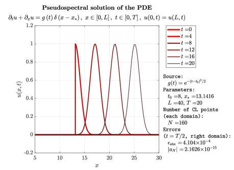
This precise problem is treated in Ref. petersson_discretizing_2016 using a (polynomial) delta function approximation procedure, with the following: $g(t)={\rm e}^{-(t-t_{0})^{2}/2}$, $t_{0}=8$, $L=40$ and $x_{*}=10+\pi$. We numerically implement the exact same setup, but using our PwP method: that is, we decompose $u=u^{-}\Theta^{-}+u^{+}\Theta^{+}$ where $\Theta^{\pm}=\Theta(\pm(x-x_{*}))$. Inserting this into (65), we get homogeneous PDEs $\partial_{t}u^{\pm}+\partial_{x}u^{\pm}=0$ to the left and right of the singularity, i.e. on $x\in\mathscr{D}^{-}=[0,x_{*}]$ and $x\in\mathscr{D}^{+}=[x_{*},L]$ respectively, along with a jump in the solution $[u]_{*}=g(t)$ at the point of the source singularity.

The details of our numerical scheme are described in Appendix C.1. We also offer in Appendix B a brief description of the PSC methods and notation used therein.

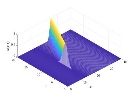
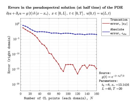
The solution for zero initial data is displayed in Figure 1, and the numerical convergence in Figure 2. For the latter, we plot—for the numerical solution $\bm{u}$ at $t=T/2$—both the absolute error (in the $l^{2}$ norm on the CL grids, as in Ref. petersson_discretizing_2016 ), $\epsilon_{{\text{abs}}}=||\bm{u}-\bm{u}_{{\text{ex}}}||_{2}$, as well as the truncation error in the right CL domain $\mathscr{D}^{+}$ given simply the absolute value of the last spectral coefficient $a_{N}$ of $\bm{u}^{+}$. We see that the truncation error exhibits typical (exponential) spectral convergence; the absolute error converges at the same rate until $N\approx 40$, after which it converges more slowly because it becomes dominated by the $\mathcal{O}(\mathrm{\Delta}t)=\mathcal{O}(N^{-2})$ error in the finite difference time evolution scheme. Nevertheless, for the same number of grid points, our procedure still yields a lower order of magnitude of the $l^{2}$ error as was obtained in Ref. petersson_discretizing_2016 with a sixth order finite difference scheme (relying on a a source discretization with 6 moment conditions and 6 smoothness conditions); we present a simple comparison of these in the following table:

$\epsilon_{\text{abs}}$	$N=80$	$N=160$
Ref. petersson_discretizing_2016	$\mathcal{O}(10^{-2})$	$\mathcal{O}(10^{-3})$
PwP method	$\mathcal{O}(10^{-3})$	$\mathcal{O}(10^{-4})$

Figure 1: Solution of the problem (65) with zero initial data.

Figure 2: Convergence of the numerical scheme for the problem (65).

4.2 Advection-type equations in neuroscience

Advection-type equations with distributional sources arise in practice, for example, in the modeling of neural populations. In particular, among the simplest of these are the so-called “integrate-and-fire” models. For some of the earlier work on such models from a neuroscience perspective, see for example haskell_population_2001 ; casti_population_2002 and references therein; for more recent work focusing on mathematical aspects, see caceres_analysis_2011 ; caceres_blow-up_2016 . Their aim is to describe the probability density $\rho\left(\bm{v},t\right)$ of neurons as a function of certain state variables $\bm{v}$ and time $t$. Often the detailed construction of these models can be quite involved and dependent on a large number of parameters, so to simply illustrate the principle of our method we here consider the simple case where the single state variable is the voltage $V$. Then, generally speaking, the dynamics of $\rho(V,t)$ takes the form of a Fokker-Planck-type equation on $V\in(-\infty,L]$ with a singular source at some fixed $V=V_{*}<L$,

$$\partial_{t}\rho+\partial_{V}\left(f\left(V,N\left(t\right)\right)\rho\right)-\frac{\sigma^{2}}{2}\partial_{V}^{2}\rho=N\left(t\right)\delta\left(V-V_{*}\right)\,.$$ (67)

The source time function $N(t)$ must be such that conservation of probability, i.e. $\partial_{t}\int{\rm d}V\rho=0$, is guaranteed under homogeneous Dirichlet BCs.

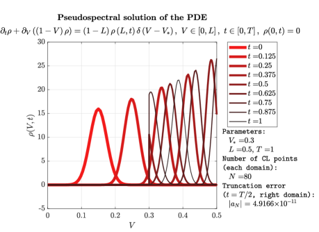
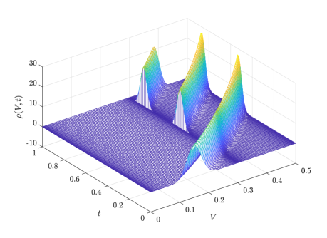
As a simplification of this problem, let us suppose, as is sometimes done, that the diffusive part (the second derivative term on the LHS) of (67) is negligible. Moreover, in simple cases, the velocity function $f$ in the advection term has the form $f=-V+{\rm constant}$, and we just work with the constant set equal to $1$. We restrict ourselves to a bounded domain for $V$ which for illustrative purposes we just choose to be $\mathscr{I}=\left[0,L\right]$. Demanding homogeneous Dirichlet BCs at the left boundary in conjunction with conservation of probability fixes the source time function to be $N(t)=(1-L)\rho(L,t)$. Thus, we are going to tackle the following problem:

$$\begin{cases}\partial_{t}\rho+\partial_{V}\left(\left(1-V\right)\rho\right)=\left(1-L\right)\rho\left(L,t\right)\delta\left(V-V_{*}\right)\,,&V\in\mathscr{I}=\left[0,L\right],t>0\,,\\ \rho\left(V,0\right)=\rho_{0}\left(V\right),\enskip\int_{\mathscr{I}}{\rm d}V\rho_{0}\left(V\right)=1\,,&\rho\left(0,t\right)=0\,.\end{cases}$$ (68)

We now implement the PwP decomposition: $\rho=\rho^{-}\Theta^{-}+\rho^{+}\Theta^{+}$ with $\Theta^{\pm}=\Theta(\pm(V-V_{*}))$. Inserting this into the PDE (68), we get the homogeneous problems $\partial_{t}\rho^{\pm}+\partial_{V}\left(\left(1-V\right)\rho^{\pm}\right)=0$ on $\mathscr{D}^{\pm}$, with $\mathscr{D}^{-}=[0,V_{*}]$ and $\mathscr{D}^{+}=[V_{*},L]$, along with the JC $[\rho]_{*}=\frac{1-L}{1-V_{*}}\rho(L,t)$.

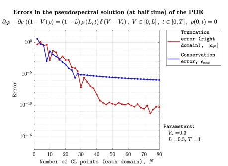
An example solution for Gaussian initial data centered at $V=0.3$ is displayed in Figure 3, and the numerical convergence in Figure 4. In the latter, we plot—again for the numerical solution $\bm{\rho}$ at the final time—the truncation error as well as (in the absence of an exact solution) what we refer to as the conservation error, $\epsilon_{{\text{cons}}}=|1-\int_{\mathscr{I}}{\rm d}V\rho(V,t)|$, which simply measures how far we are from exact conservation of probability. Both of these exhibit exponential convergence. The integral in $\epsilon_{{\text{cons}}}$ is computed as a sum over both domains, $\int_{\mathscr{I}}{\rm d}V\rho=\int_{\mathscr{D}^{-}}{\rm d}V\rho+\int_{\mathscr{D}^{+}}{\rm d}V\rho$, and numerically performed on each using a standard pseudospectral quadrature method (as in, e.g., Chapter 12 of Ref. trefethen_spectral_2001 ).

This procedure can readily be complexified with the inclusion of a diffusion term, and indeed we will shortly turn to purely diffusion (heat-type equation) problems in the following section.

Figure 3: Solution of (68) with (normalized) Gaussian initial data centered at $V=0.3$.

Figure 4: Convergence of the numerical scheme for the problem (68).

4.3 Advection-type equations in other applications

Another advection-type application in which one may be tempted to try applying some form the PwP method is the shallow water equations. Setting the gravitational acceleration to $1$, these read:

$$\partial_{t}\left[\begin{array}[]{c}h\\ hu\end{array}\right]+\partial_{x}\left[\begin{array}[]{c}hu\\ hu^{2}+\tfrac{1}{2}h^{2}\end{array}\right]=\left[\begin{array}[]{c}0\\ -h\partial_{x}B\end{array}\right]\,,$$ (69)

where $B(x)$ is the elevation of the bottom topography, $h(x,t)$ is the fluid depth above the bottom and $u(x,t)$ is the velocity. If the topography is discontinuous, i.e. if $B\notin C^{0}(\mathbb{R})$, then the RHS of (69) will be distributional; this can happen, e.g., if the bottom is a step (if $B=\Theta$, then the RHS is $\left[\begin{smallmatrix}0\\ -h\delta\end{smallmatrix}\right]$), a wall etc. However, the problem with applying the PwP method here is that (69) is nonlinear, and so one encounters precisely the sorts of issues detailed at the end of the preceding section. Indeed, explicit numerical solutions that have been obtained for (69) in the literature zhou_numerical_2002 ; bernstein_central-upwind_2016 qualitatively indicate that a PwP-type decomposition as described here would be inadequate (and, anyway, nonsensical mathematically) for such problems.

5 Parabolic PDEs

We begin by analyzing the standard heat equation and then move on to an application in finance which includes two (time-dependent) singular source terms.

5.1 Heat equation

Let us consider now the $(1+1)$-dimensional heat equation for $u(x,t)$ with a constant point source at a time-dependent location $x=x_{p}(t)$, with Dirichlet boundary conditions:

$$\begin{cases}\partial_{t}u-\partial_{x}^{2}u=\lambda\delta\left(x-x_{p}\left(t\right)\right)\,,&x\in\mathscr{I}=\left[a,b\right],\enskip t>0\,,\\ u\left(x,0\right)=0\,,&u\left(a,t\right)=\alpha,\,u\left(b,t\right)=\beta\,.\end{cases}$$ (70)

In this case, we do not have the exact solution.

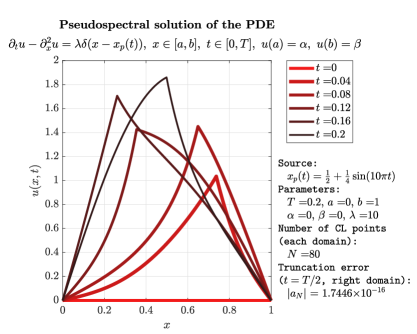
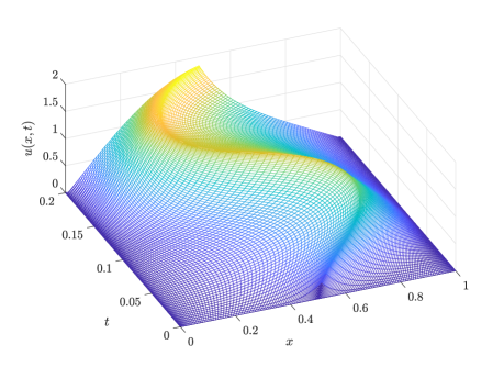
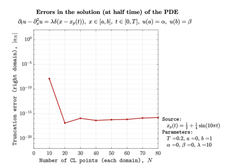
This problem is treated in tornberg_numerical_2004 using a delta function approximation procedure, with the following setup: $\mathscr{I}=[0,1]$, $\alpha=0=\beta$ and $\lambda=10$; constant-valued and sinusoidal point source locations $x_{p}(t)$ are considered. We implement here the same, using our PwP method: we decompose $u=u^{-}\Theta^{-}+u^{+}\Theta^{+}$ where $\Theta^{\pm}=\Theta(\pm(x-x_{p}(t)))$. Inserting this into (70), we get homogeneous PDEs $\partial_{t}u^{\pm}-\partial_{x}^{2}u^{\pm}=0$ to the left and right of the singularity, $x\in\mathscr{D}^{-}=[0,x_{p}(t)]$ and $x\in\mathscr{D}^{+}=[x_{p}(t),1]$ respectively; additionally, we have the following JCs: $[u]_{p}=0$ and $[\partial_{x}u]_{p}=-\lambda$.

The details of the numerical scheme are given in Appendix C.2, and results for zero initial data in Figures 5 and 6.

Figure 5: Solution of the problem (70) with zero initial data.

Figure 6: Convergence of the numerical scheme for the problem (70).

5.2 Heat-type equations in finance

We consider a model of price formation initially proposed in Ref. lasry_mean_2007 ; see also Refs. markowich_parabolic_2009 ; caffarelli_price_2011 ; burger_boltzmann-type_2013 ; achdou_partial_2014 ; pietschmann_partial_2012 . This model describes the density of buyers $f_{{\text{B}}}(x,t)$ and the density of vendors $f_{{\text{V}}}(x,t)$ in a system, as functions of of the bid or, respectively, ask price $x\in\mathbb{R}$ for a certain good being traded between them, and time $t\in[0,\infty)$.

The idea is that when a buyer and vendor agree on a price, the transaction takes place; the buyer then becomes a vendor, and vice-versa. However, it is also assumed that there exists a fixed transaction fee $a\in\mathbb{R}$. Consequently, the actual buying price is $x+a$, and so the (former) buyer will try to sell the good at the next trading event not for the price $x$, but for $x+a$. Similarly, the profit for the vendor is actually $x-a$, and so he/she would not be willing to pay more than $x-a$ for the good at the next trading event. In time, this system should achieve an equilibrium.

Mathematically, the dynamics of the buyer/vendor densities is assumed to be governed by the heat equation with a certain source term. The source term in each case is simply the (time-dependent) transaction rate $\lambda(t)$, corresponding to the flux of buyers and vendors, at the particular price where the trading event occurs, shifted accordingly by the transaction cost. Thus the system is described by

$$\begin{cases}\left(\partial_{t}-\partial_{x}^{2}\right)f_{{\text{B}}}=\lambda\left(t\right)\delta\left(x-\left(x_{p}\left(t\right)-a\right)\right)\,,&{\rm for}\,\,x<x_{p}\left(t\right)\,,\\ f_{{\text{B}}}=0\,,&{\rm for}\,\,x>x_{p}\left(t\right)\,,\end{cases}$$ (71)

and

$$\begin{cases}\left(\partial_{t}-\partial_{x}^{2}\right)f_{{\text{V}}}=\lambda\left(t\right)\delta\left(x-\left(x_{p}\left(t\right)+a\right)\right)\,,&{\rm for}\,\,x>x_{p}\left(t\right)\,,\\ f_{{\text{V}}}=0\,,&{\rm for}\,\,x<x_{p}\left(t\right)\,,\end{cases}$$ (72)

where the free boundary $x_{p}(t)$ represents the agreed price of trading at time $t$, and the transaction rate is $\lambda(t)=-\partial_{x}f_{{\text{B}}}(x_{p}(t),t)=\partial_{x}f_{{\text{V}}}(x_{p}(t),t)$. (NB: The functional form of $\lambda(t)$ is uniquely fixed simply by the requirement that the two densities are conserved, i.e. $\partial_{t}\int{\rm d}xf_{{\text{B}}}=0=\partial_{t}\int{\rm d}xf_{{\text{V}}}$, under the assumption that we have homogeneous Neumann BCs at the left and right boundaries respectively.) Now, we can actually combine this system into a single problem for the difference between buyer and vendor densities,

$$f=f_{{\text{B}}}\Theta\left(-\left(x-x_{p}\left(t\right)\right)\right)-f_{{\text{V}}}\Theta\left(x-x_{p}\left(t\right)\right)\,.$$ (73)

The “spatial” (i.e. price) domain can be taken to be bounded, and homogeneous Neumann BCs are assumed at the boundaries. Thus the problem we are interested in is:

$$\begin{cases}\partial_{t}f-\partial_{x}^{2}f=\lambda\left(t\right)\left(\delta\left(x-x_{p_{-}}\left(t\right)\right)-\delta\left(x-x_{p_{+}}\left(t\right)\right)\right)\,,&x\in\mathscr{I}=\left[0,1\right],\enskip t>0\,,\\ f\left(x,0\right)=f_{\text{I}}\left(x\right),\enskip f\gtrless 0\enskip{\rm for}\enskip x\lessgtr x_{p}\left(t\right)\,,&\partial_{x}f\left(0,t\right)=\partial_{x}f\left(1,t\right)=0\,.\end{cases}$$ (74)

where $\lambda(t)=-\partial_{x}f(x_{p}(t),t),$ and we have defined $x_{p_{\pm}}(t)=x_{p}(t)\pm a$. Moreover, one can show that from this setup, it follows that the free boundary evolves via

$$\dot{x}_{p}\left(t\right)=\frac{\partial_{x}^{2}f\left(x_{p}\left(t\right),t\right)}{\lambda\left(t\right)}\,.$$ (75)

In this case, we have not one but two singular source locations on the RHS of the PDE. Hence, in order to implement the PwP method, we must here divide the spatial domain $\mathscr{I}$ into three disjoint regions, with the two singularity locations at their interfaces: $\mathscr{I}=\mathscr{D}^{-}\cup\mathscr{D}^{0}\cup\mathscr{D}^{+}$ with $\mathscr{D}^{-}=[0,x_{p_{-}}(t)]$, $\mathscr{D}^{0}=[x_{p_{-}}(t),x_{p_{+}}(t)]$ and $\mathscr{D}^{+}=[x_{p_{+}}(t),1]$. Then, we decompose $f=f^{-}\Theta^{-}+f^{0}\Theta^{0}+f^{+}\Theta^{+}$ with $\Theta^{-}=\Theta(-(x-x_{p_{-}}(t)))$, $\Theta^{0}=\Theta(x-x_{p_{-}}(t))-\Theta(x-x_{p_{+}}(t))$ and $\Theta^{+}=\Theta(x-x_{p_{+}}(t))$. Inserting this into the PDE (74), we get homogeneous problems $(\partial_{t}-\partial_{x}^{2})f^{\sigma}=0$ on $\mathscr{D}^{\sigma}$ for $\sigma\in\{0,\pm\}$, along with the JCs $[f]_{p_{\pm}}=0$ and $[\partial_{x}f]_{p_{\pm}}=\pm\lambda(t)$.

Before proceeding to the numerical implementation, we note that it is possible to derive an exact stationary (i.e. $t\rightarrow\infty$) solution of the problem (74). In particular, denoting the (time-conserved) number of buyers and vendors, respectively, by $N_{{\text{B}}}=\int_{0}^{x_{p}}{\rm d}x\>f$ and $N_{{\text{V}}}=-\int_{x_{p}}^{1}{\rm d}x\>f$, one can show that in the stationary ($t\rightarrow\infty$) limit,

$$\begin{cases}N_{{\text{B}}}=\,&-\lambda^{\text{stat}}a(x_{p}^{\text{stat}}-a/2)\,,\\ N_{{\text{V}}}=\,&-\lambda^{\text{stat}}a(1-x_{p}^{\text{stat}}-a/2)\,,\end{cases}$$ (76)

$$\Leftrightarrow\, \begin{cases}\lambda^{\text{stat}}=\,&\left[-\left(N_{{\text{B}}}+N_{{\text{V}}}\right)\right]/\left[a\left(1-a\right)\right]\,,\\ x_{p}^{\text{stat}}=\,&\left[2N_{{\text{B}}}+a\left(N_{{\text{V}}}-N_{{\text{B}}}\right)\right]/\left[2\left(N_{{\text{B}}}+N_{{\text{V}}}\right)\right]\,,\end{cases}$$ (77)

which we can use to determine the exact stationary solution

$$\lim_{t\rightarrow\infty}f\left(x,t\right)=f^{\text{stat}}\left(x\right)=\begin{cases}-\lambda^{\text{stat}}a\,,&{\rm for}\,\,0\leq x<x_{p_{-}}^{\text{stat}}\,,\\ \lambda^{\text{stat}}\left(x-x_{p}^{\text{stat}}\right)\,,&{\rm for}\,\,x_{p_{-}}^{\text{stat}}\leq x\leq x_{p_{+}}^{\text{stat}}\,,\\ \lambda^{\text{stat}}a\,,&{\rm for}\,\,x_{p_{+}}^{\text{stat}}<x\leq 1\,.\end{cases}$$ (78)

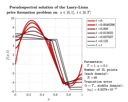
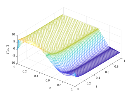
The problem (74) is solved numerically in Ref. markowich_parabolic_2009 (see also section 2.5.2 of pietschmann_partial_2012 ) using (Gaussian) delta function approximations for the source on an equispaced computational grid. We implement here using our PwP method the exact same setup: in particular, we take a transaction fee of $a=0.1$ and initial data $f_{\text{I}}(x)=\tfrac{875}{6}x^{3}-\tfrac{700}{3}x^{2}+\tfrac{175}{2}x$. (NB: Despite the fact that this does not actually satisfy homogeneous Neumann BCs, the numerical evolution will force it to.) Analytically, we have $x_{p}(0)=\tfrac{3}{5}$ and $\lambda(0)=35$. Also, using (77), we have $\lambda^{\text{stat}}=-\frac{8855}{162}$ and $x_{p}^{\text{stat}}=\frac{731}{1012}\approx 0.7223$. As we evolve forward in time, we use Chebyshev polynomial interpolation to determine the transaction rate $\lambda(t)$ (i.e. the negative of the spatial derivative of the solution at $x_{p}(t)$) as well as the evolution of $x_{p}(t)$ via (75).

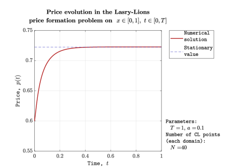
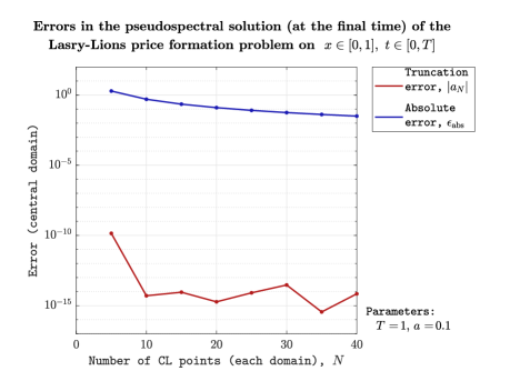
The numerical scheme is given in Appendix C.2, and results in Figures 7 and 8. In particular, in Figure 7 we show the numerical solution for $f$, and in Figure 8, the price as a function of time as well as the numerical convergence rates. For the latter, we plot not only the truncation error but also the absolute error with the stationary solution (78), in this case, using the infinity norm: $\epsilon_{\text{abs}}=||\bm{f}-\bm{f}^{\text{stat}}||_{\infty}$. Of course, since we can only evolve the solution up to a finite time (which we choose to be $t=T=1$), we should not expect this to converge to zero; however, its decline with increasing $N$ nevertheless serves to illustrate a good validation of our results.

We remark that our numerical implementation here not only requires an order of magnitude fewer grid points than that of Ref. markowich_parabolic_2009 , but in fact yields convergence to the correct stationary solution while that of Ref. markowich_parabolic_2009 does not. Indeed, in the latter, not only are more points required (essentially due to the necessity of resolving well enough the Gaussian-approximated delta functions) but the scheme actually fails, even so, to approach (78) as well as ours by the same finite time, $t=T=1$. (To wit, Ref. markowich_parabolic_2009 obtains $x_{p}\rightarrow 0.71$ in the large $t$ limit, instead of the correct value, $0.7223$, which we achieve with our PwP method as shown in Figure 8.)

Figure 7: Solution of the problem (74).

Figure 8: Price evolution and convergence of the numerical scheme for the problem (74).

6 Second order hyperbolic PDEs

We move on to consider in this section second order hyperbolic problems. In particular, we first solve the standard $(1+1)$-dimensional elastic wave equation, taking a delta derivative source. Afterwards, we discuss possible physical applications of this and obstacles thereto—including problems in gravitational physics and seismology.

6.1 Wave equation

Let us consider the the elastic wave equation, in the form of the following simplified $(1+1)$-dimensional problem for $u(x,t)$ with a delta function derivative source at a fixed point $x_{*}\in\mathscr{I}=[0,L]$, and homogeneous Dirichlet boundary conditions:

$$\begin{cases}\partial_{t}^{2}u-\partial_{x}^{2}u=g\left(t\right)\delta^{\prime}\left(x-x_{*}\right)\,,&x\in\mathscr{I}=\left[0,L\right]\,,\enskip t>0\,,\\ u\left(x,0\right)=0\,,\enskip\partial_{t}u\left(x,0\right)=0\,,&u\left(0,t\right)=0=u\left(L,t\right)\,.\end{cases}$$ (79)

It is actually possible to derive an exact solution for this problem on an unbounded domain $\mathscr{I}=\mathbb{R}$. For the interested reader, the procedure is explained in Appendix D. For concreteness we take a simple sinusoidal source time function $g(t)=\kappa\sin(\omega t)$, in which case the exact solution reads:

$$u_{{\text{ex}}}\left(x,t\right)=\, \kappa\bigg{[}\frac{1}{4}\sum_{\sigma=\pm}\sigma{\rm sgn}\left(x-x_{*}+\sigma t\right)\sin\left(\omega\left(x-x_{*}+\sigma t\right)\right)$$

$$-\frac{1}{2}{\rm sgn}\left(x-x_{*}\right)\cos\left(\omega\left(x-x_{*}\right)\right)\sin\left(\omega t\right)\bigg{]}\,,$$ (80)

where ${\rm sgn}(\cdot)$ is the sign function, with the property ${\rm d}({\rm sgn}(x))/{\rm d}x=2{\rm d}\Theta(x)/{\rm d}x=2\delta(x)$.

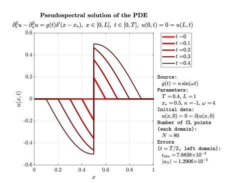
To solve (79) numerically, we implement the now familiar PwP decomposition: $u=u^{-}\Theta^{-}+u^{+}\Theta^{+}$ where $\Theta^{\pm}=\Theta(\pm(x-x_{*}))$. Inserting this into (79), we get homogeneous PDEs $\partial_{t}^{2}u^{\pm}-\partial_{x}^{2}u^{\pm}=0$ to the left and right of the singularity, $x\in\mathscr{D}^{-}=[0,x_{*}]$ and $x\in\mathscr{D}^{+}=[x_{*},L]$ respectively, along with the JCs $[u]_{p}=-g(t)$ and $[\partial_{x}u]_{p}=0$. We now proceed by recasting (79) as a first-order hyperbolic system for $\vec{U}=[u\enskip v\enskip w]^{{\rm T}}$ with $v=\partial_{x}u$ and $w=\partial_{t}u$, as

$$\partial_{t}\vec{U}=\left[\begin{array}[]{ccc}0&0&0\\ 0&0&1\\ 0&1&0\end{array}\right]\partial_{x}\vec{U}+\left[\begin{array}[]{ccc}0&0&1\\ 0&0&0\\ 0&0&0\end{array}\right]\vec{U}\quad{\rm on}\enskip\mathscr{D}^{\pm}\,,\quad\left[\vec{U}\right]_{p}=\left[\begin{array}[]{c}-g\\ 0\\ -\dot{g}\end{array}\right]\,.$$ (81)

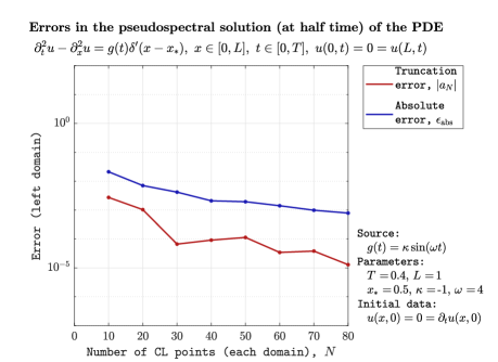
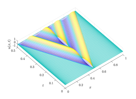
The numerical scheme is given in Appendix C.3, and results in Figures 9 and 10. The absolute error is again computed in the infinity norm on the CL grids: $\epsilon_{\text{abs}}=||\bm{u}-\bm{u}_{\text{ex}}||_{\infty}$.

The same problem (79) is considered numerically in Ref. petersson_stable_2010 , but using a different (polynomial) source function $g(t)$, and a discretization procedure for the delta function (derivatives) on the computational grid (carried out in such a way that the distributional action thereof yields the expected result on polynomials up to a given degree). With our PwP method here, we obtain the same order of magnitude of the (absolute) error in the numerical solution as that in Ref. petersson_stable_2010 for the same (order of magnitude of) number of grid points; however the drawback of the “discretized delta” method of Ref. petersson_stable_2010 , in contrast to the PwP method, is that the solution in the former is visibly quite poorly resolved close to the singularity.

We add that we have also carried out the solution to the problem shown in Figure 9 using higher-order (from second up to eighth order) finite-difference time evolution schemes. These yield no visible improvement (at any order tried) in either the absolute or the truncation error relative to the first-order time evolution results. Thus the spacial pseudospectral grid appears to control the total level of the error, with a higher-order scheme for the time evolution producing, at least in this case, no greater benefits.

Figure 9: Solution and convergence of the numerical scheme for the problem (79).

Figure 10: Solution (with $N=80$) of the same problem as in Figure 9 but using $\omega=24$.

6.2 Wave-type equations in physical applications

As we have mentioned, our numerical studies in this paper are largely motivated by their applicability to the computation of the self-force in gravitational physics. There one encounters different levels of complexity of this problem, the simplest being that of the self-force due to a scalar field—as a conceptual testbed for the more complicated and realistic problem of the full self-force of the gravitational field—in a fixed (non-dynamical) black hole spacetime. This can refer to a non-spinning (Schwarzschild-Droste) black hole, where the problem is of the form (1) where $\mathcal{L}=\partial_{t}^{2}-\partial_{x}^{2}+V$ is just a simple $(1+1)$-dimensional wave operator with some known potential $V$ and a source $S=f\delta_{(p)}$, with $\dim(\mathscr{I})=1$. We recognize this now as quite typical for the application of our PwP method, and indeed this has been done with success in the past canizares_extreme-mass-ratio_2011 ; canizares_efficient_2009 ; canizares_pseudospectral_2010 ; canizares_time-domain_2011 ; canizares_tuning_2011 ; jaramillo_are_2011 ; canizares_overcoming_2014 ; oltean_frequency-domain_2017 . As we briefly remarked in the Introduction, the main difference between most of these works and our numerical schemes throughout this paper is that for the time evolution, rather than relying on finite-difference methods, the former made use of the method of lines. This can be quite well-suited especially for these types of $(1+1)$-dimensional hyperbolic problems, which can be formulated in terms of characteristic fields propagating along the two lightcone directions ($t\pm x={\textrm{const.}}$). The imposition of the JCs is then achieved quite simply in this setting by just evolving, in the left domain, the characteristic field propagating towards the right and relating it (via the JC) to the value of the characteristic field propagating towards the left in the right domain. For the interested reader, this kind of procedure is described in detail in Chapter 3 of Ref. canizares_extreme-mass-ratio_2011 .

We could also consider the scalar self-force problem in a spinning (Kerr) black hole spacetime, however the issue there—owing to the existence of fewer symmetries in the problem than in the non-spinning case—is that $\dim(\mathscr{I})=2$ in the time domain (with a more complicated second-order hyperbolic operator $\mathcal{L}$); however, this could be remedied for a possible PwP implementation by passing to the frequency domain, which transforms (1) to an ODE (with $\dim(\mathscr{I})=1$, $\mathscr{V}=\emptyset$, and again, a simple source $S=f\delta_{(p)}$).

The application of the PwP method to the full gravitational self-force is a subject of ongoing work, however (modulo certain technical problems relating to the gauge choice, which we will not elaborate upon here) in the Schwarzschild-Droste case it essentially reduces to solving the same type of problem (1) with $\dim(\mathscr{I})=1$ and $S=f\delta_{(p)}+g\delta^{\prime}_{(p)}$. The equivalent problem in the Kerr case once again suffers from the issue that $\dim(\mathscr{I})=2$ in the time domain, so the PwP method cannot be applied there except after a transformation to the frequency domain (which produces $\dim(\mathscr{I})=1$ and $S=f\delta_{(p)}+g\delta^{\prime}_{(p)}+h\delta^{\prime\prime}_{(p)}$ in this case).

Outside of gravitational physics, another setting where the PwP technique could also possibly prove useful is in seismology. There, however, the modeling of seismic waves romanowicz_seismology_2007 ; aki_quantitative_2009 ; shearer_introduction_2009 ; madariaga_seismic_2007 ; petersson_stable_2010 typically involves equations of the form (61) with $3$-dimensional delta functions (i.e. $\dim(\mathscr{I})=\bar{n}=3$, usually referring to the $3$ dimensions of ordinary space) which, as we have amply discussed in relation thereto, are not directly amenable to a PwP-type approach as such. However, the methods outlined in this paper might be of some use if symmetries or other simplifying assumptions can, in a situation of interest, reduce the dimension of the distributional source to $1$ (as an alternative to delta function approximation procedures, which are common practice in this area as well).

7 Elliptic PDEs

Finally, we consider in this section the elliptical problem appearing in section 4.3 of Ref. tornberg_numerical_2004 : namely, the Poisson equation on a square of side length $2$ centered on the origin in $\mathbb{R}^{2}$, with a simple (negative) one-dimensional delta function source supported on the circle of radius $r_{*}=\tfrac{1}{2}$,

$$\begin{cases}\triangle_{\mathbb{R}^{2}}u=-\delta\left(r-r_{*}\right)\,,&\text{on }\mathscr{U}=\left[-1,1\right]\times\left[-1,1\right]\subset\mathbb{R}^{2}\,,\\ u=1-\tfrac{1}{2}\log\left(2r\right)\,,&\text{on }\partial\mathscr{U}\,.\end{cases}$$ (82)

In this case, the polar symmetry of the PDE entails that the solution will only depend on the radial coordinate $r$ (which in this case notationally substitutes the $x$ coordinate in antecedent sections). Indeed, (82) has an exact solution which is simply given by

$$u_{\text{ex}}=1-\tfrac{1}{2}\log\left(2r\right)\Theta\left(r-r_{*}\right)\,.$$ (83)

We can use the fact that in polar coordinates, $\triangle_{\mathbb{R}^{2}}=\partial_{r}^{2}+\tfrac{1}{r}\partial_{r}+\tfrac{1}{r^{2}}\partial_{\theta}^{2}$, and so numerically all we need to do is solve $(\partial_{r}^{2}+\tfrac{1}{r}\partial_{r})u(r)=-\delta(r-r_{*})$ for a given $\theta\in[0,2\pi]$, where the value of $\theta$ will determine $\{r\}=\mathscr{I}=[0,L]$ and hence the BC at $u(L)$ (that is, on $\partial\mathscr{U}$), and repeat over some set of discrete $\theta$ values in case the entire numerical solution on the $(r,\theta)$-plane is desired.

Thus, we simply implement the PwP method here by writing $u=u^{-}\Theta^{-}+u^{+}\Theta^{+}$ for $\Theta^{\pm}=\Theta(r-r_{*})$, whereby we obtain the homogeneous equations $(\partial_{r}^{2}+\tfrac{1}{r}\partial_{r})u^{\pm}=0$ along with the JCs $[u]_{*}=0$ and $[\partial_{r}u]_{*}=-1$.

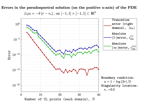
The detailed numerical scheme is given in Appendix C.4, and results in Figure 11. In this case, we simply plot the errors along the positive $x$-axis in $\mathbb{R}^{2}$ on the CL grids: in addition to the right-domain truncation error, we also show (as is done in Ref. tornberg_numerical_2004 ) the absolute error in both the $l^{1}$-norm, $\epsilon_{\text{abs}}^{(1)}=||\bm{u}-\bm{u}_{\text{ex}}||_{1}$, as well as in the infinity norm, $\epsilon_{\text{abs}}^{(\infty)}=||\bm{u}-\bm{u}_{\text{ex}}||_{\infty}$. Up to $N\approx 20$, we observe the typical (exponential) spectral convergence of all three errors, with a significant (by a few orders of magnitude) improvement over the results of Ref. tornberg_numerical_2004 (using delta function approximations) for the latter two.

Figure 11: Convergence of the pseudospectral numerical scheme for the problem (82).

8 Conclusions

We have expounded in this paper a practical approach—the “Particle-without-Particle” (PwP) method—for numerically solving differential equations with distributional sources; to summarize, one does this by breaking up the solution into (regular function) pieces supported between—plus, if necessary, at—singularity (“particle”) locations, solving sourceless (homogeneous) problems for these pieces, and then matching them via the appropriate “jump” (boundary) conditions effectively substituting the original singular source. Building upon its successful prior application in the specific context of the self-force problem in general relativity, we have here generalized this method and have shown it to be viable for any linear partial differential equation of arbitrary order, with the provision that the distributional source is supported only on a one-dimensional subspace of the total problem domain. Accordingly, we have demonstrated its usefulness by solving first and second order hyperbolic problems, with applications in neuroscience and acoustics, respectively; parabolic problems, with applications in finance; and finally a simple elliptic problem. In particular, the numerical schemes we have employed for carrying these out have been based on pseudospectral collocation methods on Chebyshev-Lobatto grids. Generally speaking, our results have yielded varying degrees of improvement in the numerical convergence rates relative to other methods in the literature that have been attempted for solving these problems (typically relying on delta function approximation procedures on the computational grid).

We stress once more that the main limitations of the our PwP method as developed here are that it is only applicable to linear problems with one-dimensionally supported distributional sources. Thus, interesting lines of inquiry for future work might be to explore—however/if at all possible—extensions or adaptations of these ideas (a) to nonlinear PDEs, which would require working with nonlinear theories of distributions (having potential applicability to problems such as, e.g., the shallow-water equations with discontinuous bottom topography); (b) to more complicated sources than the sorts considered in this paper, perhaps even containing higher-dimensional distributions but possibly also requiring additional assumptions, such as symmetries (which might be useful for problems such as, e.g., seismology models with three-dimensional delta function sources).

Appendix A Proof of distributional identity

The base case ($n=0$) reads $f(x,\mathbf{y})\delta(x-x_{p})\equiv f_{p}\delta(x-x_{p})$. It is trivial to see that this holds.

Now assume the identity holds for $n=k$. Then we must prove that it holds for $n=k+1$. In other words, we wish to show that:

$$\left\langle f\delta_{\left(p\right)}^{\left(k+1\right)},\phi\right\rangle=\left\langle\left(-1\right)^{n}\sum_{j=0}^{n}\left(-1\right)^{j}\binom{n}{j}f_{p}^{\left(n-j\right)}\delta_{\left(p\right)}^{\left(j\right)},\phi\right\rangle.$$ (84)

We begin with the LHS, and compute:

$$\left\langle f\delta_{\left(p\right)}^{\left(k+1\right)},\phi\right\rangle=\, \int_{\mathscr{I}}{\rm d}x\,f\left(x,\mathbf{y}\right)\delta_{\left(p\right)}^{\left(k+1\right)}\left(x\right)\phi\left(x\right)$$ (85)

$$=\, -\int_{\mathscr{I}}{\rm d}x\,\left(\phi^{\prime}\left(x\right)f\left(x,\mathbf{y}\right)+\phi\left(x\right)f^{{}^{\prime}}\left(x,\mathbf{y}\right)\right)\delta_{\left(p\right)}^{\left(k\right)}\left(x\right),$$ (86)

using integration by parts. Now, inserting the induction hypothesis,

$$\left\langle f\delta_{\left(p\right)}^{\left(k+1\right)},\phi\right\rangle=\, -\int_{\mathscr{I}}{\rm d}x\,\bigg{\{}\phi^{\prime}\left(x\right)\left(-1\right)^{k}\sum_{j=0}^{k}\left(-1\right)^{j}\binom{k}{j}f_{p}^{\left(k-j\right)}\delta_{\left(p\right)}^{\left(j\right)}\left(x\right)$$

$$+\phi\left(x\right)\left(-1\right)^{k}\sum_{l=0}^{k}\left(-1\right)^{l}\binom{k}{l}f_{p}^{\left(k+1-l\right)}\delta_{\left(p\right)}^{\left(j\right)}\left(x\right)\bigg{\}}$$ (87)

$$=\, \left(-1\right)^{k+1}\bigg{\{}\sum_{j=0}^{k}\left(-1\right)^{j}\binom{k}{j}f_{p}^{\left(k-j\right)}\int_{\mathscr{I}}{\rm d}x\,\phi^{\prime}\left(x\right)\delta_{\left(p\right)}^{\left(j\right)}\left(x\right)$$

$$+\sum_{l=0}^{k}\left(-1\right)^{l}\binom{k}{l}f_{p}^{\left(k+1-l\right)}\int_{\mathscr{I}}{\rm d}x\,\phi\left(x\right)\delta_{\left(p\right)}^{\left(l\right)}\left(x\right)\bigg{\}}$$ (88)

Observe that, via integration by parts, $\langle\delta_{\left(p\right)}^{\left(j\right)},\phi\rangle=(-1)^{j}\phi_{p}^{\left(j\right)}$. Hence, the above simplifies to:

$$\left\langle f\delta_{\left(p\right)}^{\left(k+1\right)},\phi\right\rangle=\, \left(-1\right)^{k+1}\bigg{\{}\sum_{j=0}^{k}\binom{k}{j}f_{p}^{\left(k-j\right)}\phi_{p}^{\left(j+1\right)}+\sum_{l=0}^{k}\binom{k}{l}f_{p}^{\left(k+1-l\right)}\phi_{p}^{\left(l\right)}\bigg{\}}$$ (89)

$$=\, \left(-1\right)^{k+1}\bigg{\{}\sum_{j=1}^{k+1}\binom{k}{j-1}f_{p}^{\left(k+1-j\right)}\phi_{p}^{\left(j\right)}+\sum_{l=0}^{k}\binom{k}{l}f_{p}^{\left(k+1-l\right)}\phi_{p}^{\left(l\right)}\bigg{\}}$$ (90)

$$=\, \left(-1\right)^{k+1}\bigg{\{}f_{p}^{\left(k+1\right)}\phi_{p}+\sum_{j=1}^{k+1}\left[\binom{k}{j-1}+\binom{k}{j}\right]f_{p}^{\left(k+1-j\right)}\phi_{p}^{\left(j\right)}+f_{p}\phi_{p}^{\left(k+1\right)}\bigg{\}}$$ (91)

after rearranging the sum terms. Using the recursive formula for the binomial coefficient, $\binom{k}{j-1}+\binom{k}{j}=\binom{k+1}{j}$, and then including the first and last terms in (91) into the sum, we get:

$$\left\langle f\delta_{\left(p\right)}^{\left(k+1\right)},\phi\right\rangle=\left(-1\right)^{k+1}\sum_{j=0}^{k+1}\binom{k+1}{j}f_{p}^{\left(k+1-j\right)}\phi_{p}^{\left(j\right)}.$$ (92)

Now using $\phi_{p}^{\left(j\right)}=\langle\delta_{\left(p\right)},\phi^{\left(j\right)}\rangle=(-1)^{j}\langle\delta_{\left(p\right)}^{\left(j\right)},\phi\rangle$, we finally obtain

$$\left\langle f\delta_{\left(p\right)}^{\left(k+1\right)},\phi\right\rangle=\, \int_{\mathscr{I}}{\rm d}x\,\phi\left(x\right)\bigg{[}\left(-1\right)^{k+1}\sum_{j=0}^{k+1}\left(-1\right)^{j}\binom{k+1}{j}f_{p}^{\left(k+1-j\right)}\delta_{\left(p\right)}^{\left(j\right)}\left(x\right)\bigg{]}$$ (93)

$$=\, \left\langle\left(-1\right)^{k+1}\sum_{j=0}^{k+1}\left(-1\right)^{j}\binom{k+1}{j}f_{p}^{\left(k+1-j\right)}\delta_{\left(p\right)}^{\left(j\right)},\phi\right\rangle,$$ (94)

which is what we wanted to prove.

Appendix B Pseudospectral collocation methods

We use this appendix to describe very cursorily the PSC methods used for the numerical schemes in this paper and to introduce some notation in relation thereto. For good detailed expositions see, for example, Refs. boyd_chebyshev_2001 ; trefethen_spectral_2001 ; peyret_chebyshev_2002 .

We work on Chebyshev-Lobatto (CL) computational grids. On any domain $[a,b]=\mathscr{D}\subseteq\mathscr{I}$, these comprise the (non-uniformly spaced) set of $N$ points $\{X_{i}\}_{i=0}^{N}\subset\mathscr{D}$ obtained by projecting onto $\mathscr{D}$ those points located at equal angles on a hypothetical semicircle having $\mathscr{D}$ as its diameter. That is to say, the CL grid on the “standard” spectral domain $\mathscr{D}^{\text{s}}=[-1,1]$ is given by

$$X_{i}^{\text{s}}=-\cos\left(\frac{\pi i}{N}\right)\,,\quad\forall 0\leq i\leq N\,,$$ (95)

which can straightforwardly be transformed (by shifting and stretching) to the desired grid on $\mathscr{D}$. For any function $f:\mathscr{D}\rightarrow\mathbb{R}$ we denote via a subscript its value at the $i$-th CL point, $f(X_{i})=f_{i}$, and in slanted boldface the vector containing all such values,

$$\bm{f}=\left[\begin{array}[]{c}f_{0}\\ f_{1}\\ \vdots\\ f_{N}\end{array}\right]\,.$$ (96)

There exists an $(N+1)\times(N+1)$ matrix $\mathbb{D}$, the so-called CL differentiation matrix, such that the derivative values of $f$ can be approximated simply by applying it to (96), i.e. $\bm{f}^{\prime}=\mathbb{D}\bm{f}$. For convenience, we also employ the notation $\mathbb{M}(r_{\text{i}}:r_{\text{f}},c_{\text{i}}:c_{\text{f}})$ to refer to the part of any matrix $\mathbb{M}$ from the $r_{\text{i}}$-th to the $r_{\text{f}}$-th row and from the $c_{\text{i}}$-th to the $c_{\text{f}}$-th column. (A simple “$:$” indicates taking all rows/columns.)

Appendix C Numerical schemes for distributionally-sourced PDEs

C.1 First-order hyperbolic PDEs

We apply a first order in time finite difference scheme to the homogeneous PDEs; thus, prior to imposing BCs/JCs, the equations become $\frac{1}{\mathrm{\Delta}t}(\bm{u}_{k+1}^{\pm}-\bm{u}_{k}^{\pm})=-\mathbb{D}^{\pm}\bm{u}_{k}^{\pm}$, where the vectors $\bm{u}_{k}^{\pm}$ contain the values of the solutions on the CL grids at the $k$-th time step, $\mathbb{D}^{\pm}$ is the CL differentiation matrix on the respective domains, and $\mathrm{\Delta}t$ is our time step. We can rewrite the discretized PDE as $\bm{u}_{k+1}^{\pm}=\bm{u}_{k}^{\pm}-\mathrm{\Delta}t\mathbb{D}^{\pm}\bm{u}_{k}^{\pm}=\bm{s}_{k}^{\pm}$. To impose the BC and JC, we modify the equations as follows:

$$\left[\begin{array}[]{c}\bm{u}_{k+1}^{-}\\ \hline\cr\bm{u}_{k+1}^{+}\end{array}\right]=\left[\begin{array}[]{c}u_{N,k}^{+}\\ \bm{s}_{k}^{-}(2:N+1)\\ \hline\cr u_{N,k}^{-}+g_{k}\\ \bm{s}_{k}^{+}(2:N+1)\end{array}\right].$$ (97)

Similarly, for our neuroscience application, we discretize the PDE using a first order finite difference scheme: $\frac{1}{\mathrm{\Delta}t}(\bm{\rho}_{k+1}^{\pm}-\bm{\rho}_{k}^{\pm})=-\mathbb{D}^{\pm}\bm{R}_{k}^{\pm}$ where $R_{i,k}^{\pm}=(1-V_{i}^{\pm})\rho_{i,k}^{\pm}$. Hence, prior to imposing the BC/JC, we have $\bm{\rho}_{k+1}^{\pm}=\bm{\rho}_{k}^{\pm}-\mathrm{\Delta}t\mathbb{D}^{\pm}\bm{R}_{k}^{\pm}=\bm{s}_{k}^{\pm}$. To impose the BC/JC, we just modify the equations accordingly:

$$\left[\begin{array}[]{c}\bm{\rho}_{k+1}^{-}\\ \hline\cr\bm{\rho}_{k+1}^{+}\end{array}\right]=\left[\begin{array}[]{c}0\\ \bm{s}_{k}^{-}(2:N+1)\\ \hline\cr\rho_{N,k}^{-}+\frac{1-L}{1-V_{*}}\rho_{N,k}^{+}\\ \bm{s}_{k}^{+}(2:N+1)\end{array}\right].$$ (98)

C.2 Parabolic PDEs

In these problems, we have moving boundaries for the CL grids (since the location of the singular source is time-dependent). The mapping for transforming the standard (fixed) spectral domain $[-1,1]$ into an arbitrary (time-dependent) one, say $\mathscr{D}=[a(t),b(t)]$, is given by

$$\mathscr{V}\times\left[0,1\right]\rightarrow\, \mathscr{V}\times\mathscr{D}$$ (99)

$$\left(T,X\right)\mapsto\, \left(t\left(T\right),x\left(T,X\right)\right)\,,$$ (100)

where

$$t\left(T\right)=\, T\,,$$ (101)

$$x\left(T,X\right)=\, \frac{b-a}{2}X+\frac{a+b}{2}\,.$$ (102)

For transforming back, we have

$$\mathscr{V}\times\mathscr{D}\rightarrow\, \mathscr{V}\times\left[0,1\right]$$ (103)

$$\left(t,x\right)\mapsto\, \left(T\left(t\right),X\left(t,x\right)\right)\,,$$ (104)

where

$$T\left(t\right)=\, t\,,$$ (105)

$$X\left(t,x\right)=\, \frac{2x-a-b}{b-a}\,.$$ (106)

Thus, for any function $f(t,x)$ in these problems, we must take care to express the time partial using the chain rule as

$$\frac{\partial f}{\partial t}=\, \frac{\partial f}{\partial T}\frac{\partial T}{\partial t}+\frac{\partial f}{\partial X}\frac{\partial X}{\partial t}$$ (107)

$$=\, \frac{\partial f}{\partial T}-\frac{2}{\left(b-a\right)^{2}}\left[\left(b-x\right)\dot{a}+\left(x-a\right)\dot{b}\right]\frac{\partial f}{\partial X}\,,$$ (108)

where in the second line we have used (105)-(106).

Now, let us use this to formulate the numerical schemes for our problems—first, for the heat equation. Let $\mathbb{D}_{k}^{\pm}$ denote the CL differentiation matrices on each of the two domains at the $k$-th time step. Then, using (108), we have here the following finite difference formula for the homogeneous PDEs prior to imposing BCs/JCs: $\frac{1}{\mathrm{\Delta}t}(\bm{u}_{k+1}^{\pm}-\bm{u}_{k}^{\pm})=(\mathbb{D}_{k}^{\pm})^{2}\bm{u}_{k}^{\pm}-\mathbb{C}_{k}^{\pm}\mathbb{D}\bm{u}_{k}^{\pm}$, where $\mathbb{D}$ is the CL differentiation matrix on $[-1,1]$ and $\mathbb{C}_{k}^{-}={\rm diag}([2/(x_{p}(t_{k}))^{2}][(-x_{i}^{-})\dot{x}_{p}(t_{k})])$, $\mathbb{C}_{k}^{+}={\rm diag}([2/(1-x_{p}(t_{k}))^{2}][(x_{i}^{+}-1)\dot{x}_{p}(t_{k})])$. Thus $\bm{u}_{k+1}^{\pm}=\bm{u}_{k}^{\pm}+\mathrm{\Delta}t[(\mathbb{D}_{k}^{\pm})^{2}-\mathbb{C}_{k}^{\pm}\mathbb{D}]\bm{u}_{k}^{\pm}=\bm{s}_{k}^{\pm}$. We can implement the BCs and JCs, by modifying the first and last equations on each domain:

$$\left[\begin{array}[]{cccc|cccc}1&0&\cdots&0&0\\ 0&1&\cdots&0&&0\\ \vdots&\vdots&\ddots&\vdots&&&\ddots\\ 0&0&\cdots&1&&&&0\\ \hline\cr 0&&&&&&\mathbb{D}_{k}^{+}(1,:)\\ &0&&&0&1&\cdots&0\\ &&\ddots&&\vdots&\vdots&\ddots&\vdots\\ &&&0&0&0&\cdots&1\end{array}\right]\left[\begin{array}[]{c}\\ \bm{u}_{k+1}^{-}\\ \\ \hline\cr\\ \bm{u}_{k+1}^{+}\\ \\ \end{array}\right]=\left[\begin{array}[]{c}0\\ \bm{s}_{k}^{-}(2:N)\\ u_{0,k}^{+}\\ \hline\cr\mathbb{D}_{k}^{-}(N,:)\bm{u}_{k}^{-}-\lambda\\ \bm{s}_{k}^{+}(2:N)\\ 0\end{array}\right].$$ (109)

Note that we are actually introducing an error by using (for convenience and ease of adaptability) $\mathbb{D}_{k}^{+}$ instead of $\mathbb{D}_{k+1}^{+}$ on the LHS (in the equation for $u_{0,k+1}^{+}$). However, one can easily convince oneself that $\mathbb{D}_{k+1}^{+}-\mathbb{D}_{k}^{+}=\mathcal{O}(\mathrm{\Delta}t)$, which is already the order of the error of the finite difference scheme, so we are not actually introducing any new error in this way. Furthermore, because we use up the last equation for $\bm{u}_{k}^{-}$ to impose the JC on $u$ (i.e. we do not have an equation for $u_{N,k}^{-}$), we must use the derivative at the previous point (i.e., at $u_{N-1,k}^{-}$) in order to impose the derivative JC. Hence on the RHS, we use $\mathbb{D}_{k}^{-}(N,:)$ instead of $\mathbb{D}_{k}^{-}(N+1,:)$.

The scheme for the finance model is analogous. We use again the first-order finite-difference method for the homogeneous equations, $\frac{1}{\mathrm{\Delta}t}(\bm{f}_{k+1}^{\sigma}-\bm{f}_{k}^{\sigma})=(\mathbb{D}_{k}^{\sigma})^{2}\bm{f}_{k}^{\sigma}-\mathbb{C}_{k}^{\sigma}\mathbb{D}\bm{f}_{k}^{\sigma}$ with the matrices $\mathbb{C}_{k}^{\sigma}$ defined similarly to those in the heat equation problem (again using (108)); thus $\bm{f}_{k+1}^{\sigma}=\bm{f}_{k}^{\sigma}+\mathrm{\Delta}t[(\mathbb{D}_{k}^{\sigma})^{2}-\mathbb{C}_{k}^{\sigma}\mathbb{D}]\bm{f}_{k}^{\sigma}=\bm{s}_{k}^{\sigma}$. To impose the BCs/JCs, we modify the equations appropriately:

$$\left[\begin{array}[]{ccccc}&&\mathbb{D}_{k}^{-}(1,:)\\ 0&1&\cdots&0&0\\ \vdots&\vdots&\ddots&\vdots&\vdots\\ 0&0&\cdots&1&0\\ 0&0&\cdots&0&1\end{array}\right]\left[\begin{array}[]{c}\\ \\ \bm{f}_{k+1}^{-}\\ \\ \\ \end{array}\right] =\left[\begin{array}[]{c}0\\ s_{1,k}^{-}\\ \vdots\\ s_{N,k}^{-}\\ f_{0,k}^{0}\end{array}\right],$$ (125)

$$\left[\begin{array}[]{ccccc}&&\mathbb{D}_{k}^{0}(1,:)\\ 0&1&\cdots&0&0\\ \vdots&\vdots&\ddots&\vdots&\vdots\\ 0&0&\cdots&1&0\\ 0&0&\cdots&0&1\end{array}\right]\left[\begin{array}[]{c}\\ \\ \bm{f}_{k+1}^{0}\\ \\ \\ \end{array}\right] =\left[\begin{array}[]{c}\mathbb{D}_{k}^{-}(N,:)\bm{f}_{k}^{-}-\lambda_{k}\\ s_{1,k}^{0}\\ \vdots\\ s_{N,k}^{0}\\ f_{0,k}^{+}\end{array}\right],$$ (141)

$$\left[\begin{array}[]{ccccc}&&\mathbb{D}_{k}^{+}(1,:)\\ 0&1&\cdots&0&0\\ \vdots&\vdots&\ddots&\vdots&\vdots\\ 0&0&\cdots&1&0\\ &&\mathbb{D}_{k}^{+}(N+1,:)\end{array}\right]\left[\begin{array}[]{c}\\ \\ \bm{f}_{k+1}^{+}\\ \\ \\ \end{array}\right] =\left[\begin{array}[]{c}\mathbb{D}_{k}^{0}(N,:)\bm{f}_{k}^{0}+\lambda_{k}\\ s_{1,k}^{+}\\ \vdots\\ s_{N,k}^{+}\\ 0\end{array}\right].$$ (157)

C.3 Second-order hyperbolic PDEs

We again apply a first order in time finite difference scheme to the homogeneous PDEs; prior to imposing BCs/JCs, the equations become

$$\frac{1}{\mathrm{\Delta}t}\left(\left[\begin{array}[]{c}\bm{u}_{k+1}^{\pm}\\ \bm{v}_{k+1}^{\pm}\\ \bm{w}_{k+1}^{\pm}\end{array}\right]-\left[\begin{array}[]{c}\bm{u}_{k}^{\pm}\\ \bm{v}_{k}^{\pm}\\ \bm{w}_{k}^{\pm}\end{array}\right]\right)=\mathbb{C}^{\pm}\left[\begin{array}[]{c}\bm{u}_{k}^{\pm}\\ \bm{v}_{k}^{\pm}\\ \bm{w}_{k}^{\pm}\end{array}\right]\,,$$ (158)

where

$$\mathbb{C}^{\pm}=\left[\begin{array}[]{ccc}0&0&0\\ 0&0&\mathbb{I}\\ 0&\mathbb{I}&0\end{array}\right]\left[\begin{array}[]{ccc}\mathbb{D}^{\pm}&0&0\\ 0&\mathbb{D}^{\pm}&0\\ 0&0&\mathbb{D}^{\pm}\end{array}\right]+\left[\begin{array}[]{ccc}0&0&\mathbb{I}\\ 0&0&0\\ 0&0&0\end{array}\right]=\left[\begin{array}[]{ccc}0&0&\mathbb{I}\\ 0&0&\mathbb{D}^{\pm}\\ 0&\mathbb{D}^{\pm}&0\end{array}\right]\,.$$ (159)

We can rewrite the discretized PDE as

$$\left[\begin{array}[]{c}\bm{u}_{k+1}^{\pm}\\ \bm{v}_{k+1}^{\pm}\\ \bm{w}_{k+1}^{\pm}\end{array}\right]=\left(\mathrm{\Delta}t\mathbb{C}^{\pm}+\mathbb{I}\right)\left[\begin{array}[]{c}\bm{u}_{k}^{\pm}\\ \bm{v}_{k}^{\pm}\\ \bm{w}_{k}^{\pm}\end{array}\right]=\left[\begin{array}[]{c}\bm{s}_{k}^{\pm}\\ \bm{y}_{k}^{\pm}\\ \bm{z}_{k}^{\pm}\end{array}\right]\,.$$ (160)

To impose the BCs and JCs, we modify the equations as follows:

$$\left[\begin{array}[]{cccc}1&\cdots&0&0\\ \vdots&\ddots&\vdots&0\\ 0&\cdots&1&0\\ &\mathbb{D}^{-}(N+1,:)\end{array}\right]\left[\begin{array}[]{c}\\ \bm{u}_{k+1}^{-}\\ \\ \end{array}\right]=\, \left[\begin{array}[]{c}0\\ \bm{s}_{k}^{-}(2:N)\\ \mathbb{D}^{+}(1,:)\bm{u}_{k}^{+}\end{array}\right]\,,$$ (171)

$$\left[\begin{array}[]{c}\\ \bm{u}_{k+1}^{+}\\ \\ \end{array}\right]=\, \left[\begin{array}[]{c}u_{N-1,k+1}^{-}-g_{k}\\ \bm{s}_{k}^{+}(2:N)\\ 0\end{array}\right]\,,$$ (178)

$$\left[\begin{array}[]{c}\bm{v}_{k+1}^{-}\\ \hline\cr\bm{v}_{k+1}^{+}\end{array}\right]=\, \left[\begin{array}[]{c}\mathbb{D}^{-}\bm{u}_{k+1}^{-}\\ \hline\cr\mathbb{D}^{+}\bm{u}_{k+1}^{+}\end{array}\right]\,,$$ (183)

$$\left[\begin{array}[]{c}\bm{w}_{k+1}^{-}\\ \hline\cr\bm{w}_{k+1}^{+}\end{array}\right]=\, \left[\begin{array}[]{c}0\\ \bm{z}_{k}^{-}(2:N+1)\\ \hline\cr w_{N,k+1}^{-}-\dot{g}_{k+1}\\ \bm{z}_{k}^{+}(2:N)\\ 0\end{array}\right]\,,$$ (191)

C.4 Elliptic PDEs

In this case we have no time evolution, and we simply need to solve $((\mathbb{D}^{\pm})^{2}+{\rm diag}(1/X_{i}^{\pm})\mathbb{D}^{\pm})\bm{u}^{\pm}=\mathbb{M}^{\pm}\bm{u}^{\pm}={\bf 0}$, modified appropriately to account for the BCs and JCs. In particular, we first solve for $\bm{u}^{+}$ using the BCs, and then for $\bm{u}^{-}$ using the solution for $\bm{u}^{+}$ to implement the JCs:

$$\left[\begin{array}[]{c}\mathbb{M}^{+}(1:N-1,:)\\ 0\enskip 0\cdots 0\enskip 1\\ \mathbb{D}^{+}(N+1,:)\end{array}\right]\bm{u}^{+}=\, \left[\begin{array}[]{c}{\bf 0}(1:N-1)\\ 1-\tfrac{1}{2}\log(2L)\\ -\tfrac{1}{2L}\end{array}\right]\,,$$ (198)

$$\left[\begin{array}[]{c}\mathbb{M}^{-}(1:N-1,:)\\ 0\enskip 0\cdots 0\enskip 1\\ \mathbb{D}^{-}(N+1,:)\end{array}\right]\bm{u}^{-}=\, \left[\begin{array}[]{c}{\bf 0}(1:N-1)\\ u_{0}^{+}\\ \mathbb{D}^{+}(1,:)\bm{u}^{+}+1\end{array}\right]\,.$$ (205)

Appendix D Exact solution for the elastic wave equation

A useful method for obtaining exact solutions to the problem (79) on $\mathscr{I}=\mathbb{R}$ is outlined in Ref. petersson_stable_2010 ; we follow the same procedure here, except using a sinusoidal source time function (rather than a polynomial, as is done in Ref. petersson_stable_2010 ).

We begin by Fourier transforming the PDE in the spatial domain, using

$$\hat{u}\left(\xi,t\right)=\int_{\mathbb{R}}{\rm d}x\,u\left(x,t\right){\rm e}^{-{\rm i}\xi x}\,,\quad u\left(x,t\right)=\frac{1}{2\pi}\int_{\mathbb{R}}{\rm d}\xi\,\hat{u}\left(\xi,t\right){\rm e}^{{\rm i}\xi x}\,.$$ (206)

Thus, multiplying the PDE in (79) by ${\rm e}^{-{\rm i}\xi x}$, integrating over $\mathbb{R}$ and applying integration by parts with the assumption of vanishing boundary terms, we get the following equation for the Fourier transform of $u$:

$$\ddot{\hat{u}}+\xi^{2}\hat{u}={\rm i}\xi g\left(t\right){\rm e}^{-{\rm i}\xi x_{*}}\,.$$ (207)

One can easily check that the exact solution of (207), with initial conditions $\hat{u}(\xi,0)=0=\dot{\hat{u}}(\xi,0)$, is simply

$$\hat{u}\left(\xi,t\right)=\frac{1}{2}{\rm e}^{-{\rm i}\xi x_{*}}\sum_{\sigma=\pm}\sigma{\rm e}^{\sigma{\rm i}\xi t}\int_{0}^{t}{\rm d}\tau\,g\left(\tau\right){\rm e}^{-\sigma{\rm i}\xi\tau}\,.$$ (208)

Inserting $g(\tau)=\kappa\sin(\omega\tau)$ into (208) and carrying out the integrals, we get

$$\hat{u}=\frac{{\rm i}\kappa{\rm e}^{-{\rm i}\xi x_{*}}}{\xi^{2}-\omega^{2}}\left[\xi\sin\left(\omega t\right)-\omega\sin\left(\xi t\right)\right]\,.$$ (209)

Finally, plugging (209) back into (206) and using

$$\int_{\mathbb{R}}{\rm d}\xi\,\frac{\xi{\rm e}^{{\rm i}\xi\left(x-x_{*}\right)}}{\xi^{2}-\omega^{2}}=\, {\rm i}\pi{\rm sgn}\left(x-x_{*}\right)\cos\left(\omega\left(x-x_{*}\right)\right)\,,$$ (210)

$$\int_{\mathbb{R}}{\rm d}\xi\,\frac{\sin\left(\xi t\right){\rm e}^{{\rm i}\xi\left(x-x_{*}\right)}}{\xi^{2}-\omega^{2}}=\, \frac{{\rm i}\pi}{2\omega}\sum_{\sigma=\pm}\sigma{\rm sgn}\left(x-x_{*}+\sigma t\right)\sin\left(\omega\left(x-x_{*}+\sigma t\right)\right)\,,$$ (211)

we get the solution (80).

References

- (1) L. Schwartz, Théorie des distributions (Hermann, Paris, 1957)
- (2) L. Schwartz, Sur l’impossibilité de la multiplication des distributions, C. R. Acad. Sci. Paris 29, 847 (1954). URL http://sites.mathdoc.fr/OCLS/pdf/OCLS_1954__21__1_0.pdf
- (3) C.K. Li, in Mathematical Methods in Engineering (Springer, Dordrecht, 2007), pp. 71–96. URL https://link.springer.com/chapter/10.1007/978-1-4020-5678-9_5
- (4) J.F. Colombeau, Nonlinear Generalized Functions: their origin, some developments and recent advances, São Paulo J. Math. Sci. 7, 201 (2013). URL http://arxiv.org/abs/1401.4755
- (5) E. Bottazzi, Grid functions of nonstandard analysis in the theory of distributions and in partial differential equations, arXiv:1704.00470 [math] (2017). URL http://arxiv.org/abs/1704.00470
- (6) R. Geroch, J. Traschen, Strings and other distributional sources in general relativity, Phys. Rev. D 36, 1017 (1987). URL https://link.aps.org/doi/10.1103/PhysRevD.36.1017
- (7) Y. Mino, M. Sasaki, T. Tanaka, Gravitational radiation reaction to a particle motion, Phys. Rev. D 55, 3457 (1997). URL https://link.aps.org/doi/10.1103/PhysRevD.55.3457
- (8) T.C. Quinn, R.M. Wald, Axiomatic approach to electromagnetic and gravitational radiation reaction of particles in curved spacetime, Phys. Rev. D 56, 3381 (1997). URL https://link.aps.org/doi/10.1103/PhysRevD.56.3381
- (9) S. Detweiler, B.F. Whiting, Self-force via a Green’s function decomposition, Phys. Rev. D 67, 024025 (2003). URL https://link.aps.org/doi/10.1103/PhysRevD.67.024025
- (10) S.E. Gralla, R.M. Wald, A rigorous derivation of gravitational self-force, Class. Quantum Grav. 25, 205009 (2008). URL http://stacks.iop.org/0264-9381/25/i=20/a=205009
- (11) S.E. Gralla, R.M. Wald, A note on the coordinate freedom in describing the motion of particles in general relativity, Class. Quantum Grav. 28, 177001 (2011). URL http://stacks.iop.org/0264-9381/28/i=17/a=177001
- (12) E. Poisson, A. Pound, I. Vega, The Motion of Point Particles in Curved Spacetime, Living Rev. Relativ. 14, 7 (2011). URL http://relativity.livingreviews.org/Articles/lrr-2011-7/
- (13) L. Blanchet, A. Spallicci, B. Whiting (eds.), Mass and Motion in General Relativity. No. 162 in Fundamental Theories of Physics (Springer, Dordrecht, 2011). URL http://www.springer.com/gp/book/9789048130146
- (14) A.D.A.M. Spallicci, P. Ritter, S. Aoudia, Self-force driven motion in curved spacetime, Int. J. Geom. Methods Mod. Phys. 11, 1450072 (2014). URL http://www.worldscientific.com/doi/abs/10.1142/S0219887814500728
- (15) A. Pound, in Equations of Motion in Relativistic Gravity, ed. by D. Puetzfeld, C. Lämmerzahl, B. Schutz, no. 179 in Fundamental Theories of Physics (Springer, Cham, 2015), pp. 399–486. URL http://link.springer.com/chapter/10.1007/978-3-319-18335-0_13
- (16) B. Wardell, in Equations of Motion in Relativistic Gravity, ed. by D. Puetzfeld, C. Lämmerzahl, B. Schutz, no. 179 in Fundamental Theories of Physics (Springer, Cham, 2015), pp. 487–522. URL https://link.springer.com/chapter/10.1007/978-3-319-18335-0_14
- (17) P.A.M. Dirac, Classical theory of radiating electrons, Proc. Royal Soc. A: Math., Phys. and Eng. Sci. 167, 148 (1938). URL http://rspa.royalsocietypublishing.org/content/167/929/148
- (18) B.S. DeWitt, R.W. Brehme, Radiation damping in a gravitational field, Ann. Phys. 9, 220 (1960). URL http://www.sciencedirect.com/science/article/pii/0003491660900300
- (19) A.O. Barut, Electrodynamics and Classical Theory of Fields and Particles (Dover Publications, New York, 1980)
- (20) P. Amaro-Seoane et al., The Gravitational Universe, arXiv:1305.5720 [astro-ph.CO] (2013). URL http://arxiv.org/abs/1305.5720
- (21) P. Amaro-Seoane et al., Laser Interferometer Space Antenna, arXiv:1702.00786 [astro-ph] (2017). URL http://arxiv.org/abs/1702.00786
- (22) E. Haskell, D.Q. Nykamp, D. Tranchina, Population density methods for large-scale modelling of neuronal networks with realistic synaptic kinetics: cutting the dimension down to size, Network: Comput. Neural Syst. 12, 141 (2001). URL http://citeseerx.ist.psu.edu/viewdoc/download;jsessionid=92F61208FEAF49749FF4D689FB16AE83?doi=10.1.1.333.3553&rep=rep1&type=pdf
- (23) A.R.R. Casti, A. Omurtag, A. Sornborger, E. Kaplan, B. Knight, J. Victor, L. Sirovich, A population study of integrate-and-fire-or-burst neurons, Neural Computation 14, 957 (2002). URL https://www.mitpressjournals.org/doi/10.1162/089976602753633349
- (24) M.J. Cáceres, J.A. Carrillo, B. Perthame, Analysis of nonlinear noisy integrate & fire neuron models: blow-up and steady states, J. Math. Neurosci. 1, 7 (2011). URL http://mathematical-neuroscience.springeropen.com/articles/10.1186/2190-8567-1-7
- (25) M.J. Cáceres, R. Schneider, Blow-up, steady states and long time behaviour of excitatory-inhibitory nonlinear neuron models, Kinet. Relat. Mod. 10, 587 (2016). URL http://www.aimsciences.org/journals/displayArticlesnew.jsp?paperID=13531
- (26) J.M. Lasry, P.L. Lions, Mean field games, Jpn. J. Math. 2, 229 (2007). URL http://link.springer.com/article/10.1007/s11537-007-0657-8
- (27) P.A. Markowich, N. Matevosyan, J.F. Pietschmann, M.T. Wolfram, On a parabolic free boundary equation modeling price formation, Math. Models Methods Appl. Sci. 19, 1929 (2009). URL http://www.worldscientific.com/doi/abs/10.1142/S0218202509003978
- (28) L.A. Caffarelli, P.A. Markowich, J.F. Pietschmann, On a price formation free boundary model by Lasry & Lions, C. R. Acad. Sci. Paris, Ser. I 349, 621 (2011). URL http://www.sciencedirect.com/science/article/pii/S1631073X11001488
- (29) M. Burger, L. Caffarelli, P.A. Markowich, M.T. Wolfram, On a Boltzmann-type price formation model, Proc. R. Soc. A 469, 20130126 (2013). URL http://rspa.royalsocietypublishing.org/content/469/2157/20130126
- (30) Y. Achdou, F.J. Buera, J.M. Lasry, P.L. Lions, B. Moll, Partial differential equation models in macroeconomics, Phil. Trans. R. Soc. A 372, 20130397 (2014). URL http://rsta.royalsocietypublishing.org/content/372/2028/20130397
- (31) J.F. Pietschmann, On some partial differential equation models in socio-economic contexts - analysis and numerical simulations. Doctorate thesis, University of Cambridge (2012). URL https://www.repository.cam.ac.uk/handle/1810/241495
- (32) N.A. Petersson, B. Sjogreen, Stable Grid Refinement and Singular Source Discretization for Seismic Wave Simulations, Commun. Comput. Phys. 8, 1074 (2010). URL http://www.global-sci.com/issue/abstract/readabs.php?vol=8&page=1074&issue=5&ppage=1110&year=2010
- (33) M. Kaltenbacher (ed.), Computational Acoustics (Springer, New York, NY, 2017). URL http://www.springer.com/gp/book/9783319590370
- (34) B. Romanowicz, A. Dziewonski (eds.), Seismology and Structure of the Earth. Treatise on Geophysics (Elsevier, 2007)
- (35) K. Aki, P.G. Richards, Quantitative Seismology, 2nd edn. (University Science Books, Sausalito, CA, 2009)
- (36) P.M. Shearer, Introduction to Seismology, 2nd edn. (Cambridge University Press, Cambridge; New York, 2009)
- (37) R. Madariaga, in Earthquake Seismology, ed. by H. Kanamori, Treatise on Geophysics (Elsevier, 2007), pp. 59–82
- (38) A.K. Tornberg, B. Engquist, Numerical approximations of singular source terms in differential equations, J. Comput. Phys. 200, 462 (2004). URL http://www.sciencedirect.com/science/article/pii/S0021999104001767
- (39) P. Cañizares, Extreme-Mass-Ratio Inspirals. Doctorate thesis, Universitat Autònoma de Barcelona (2011). URL https://gwic.ligo.org/thesisprize/2011/canizares_thesis.pdf
- (40) P. Cañizares, C.F. Sopuerta, Efficient pseudospectral method for the computation of the self-force on a charged particle: Circular geodesics around a Schwarzschild black hole, Phys. Rev. D 79, 084020 (2009). URL http://link.aps.org/doi/10.1103/PhysRevD.79.084020
- (41) P. Cañizares, C.F. Sopuerta, J.L. Jaramillo, Pseudospectral collocation methods for the computation of the self-force on a charged particle: Generic orbits around a Schwarzschild black hole, Phys. Rev. D 82, 044023 (2010). URL http://link.aps.org/doi/10.1103/PhysRevD.82.044023
- (42) P. Cañizares, C.F. Sopuerta, Time-domain modelling of Extreme-Mass-Ratio Inspirals for the Laser Interferometer Space Antenna, J. Phys.: Conf. Ser. 314, 012075 (2011). URL http://stacks.iop.org/1742-6596/314/i=1/a=012075
- (43) P. Cañizares, C.F. Sopuerta, Tuning time-domain pseudospectral computations of the self-force on a charged scalar particle, Class. Quantum Grav. 28, 134011 (2011). URL http://stacks.iop.org/0264-9381/28/i=13/a=134011
- (44) J.L. Jaramillo, C.F. Sopuerta, P. Cañizares, Are time-domain self-force calculations contaminated by Jost solutions?, Phys. Rev. D 83, 061503 (2011). URL http://link.aps.org/doi/10.1103/PhysRevD.83.061503
- (45) P. Cañizares, C.F. Sopuerta, Overcoming the Gauge Problem for the Gravitational Self-Force, arXiv:1406.7154 [gr-qc] (2014). URL http://arxiv.org/abs/1406.7154
- (46) M. Oltean, C.F. Sopuerta, A.D.A.M. Spallicci, A frequency-domain implementation of the particle-without-particle approach to EMRIs, J. Phys.: Conf. Ser. 840, 012056 (2017). URL http://stacks.iop.org/1742-6596/840/i=1/a=012056
- (47) S. Aoudia, A.D.A.M. Spallicci, Source-free integration method for black hole perturbations and self-force computation: Radial fall, Phys. Rev. D 83, 064029 (2011). URL https://link.aps.org/doi/10.1103/PhysRevD.83.064029
- (48) P. Ritter, A.D.A.M. Spallicci, S. Aoudia, S. Cordier, A fourth-order indirect integration method for black hole perturbations: even modes, Class. Quantum Grav. 28, 134012 (2011). URL http://stacks.iop.org/0264-9381/28/i=13/a=134012
- (49) A.D.A.M. Spallicci, P. Ritter, S. Jubertie, S. Cordier, S. Aoudia, Towards a Self-consistent Orbital Evolution for EMRIs, Astron. Soc. Pac. Conf. Ser. 467, 221 (2012). URL https://arxiv.org/abs/1209.1969
- (50) A.D.A.M. Spallicci, P. Ritter, A fully relativistic radial fall, Int. J. Geom. Methods Mod. Phys. 11, 1450090 (2014). URL http://www.worldscientific.com/doi/abs/10.1142/S021988781450090X
- (51) P. Ritter, S. Aoudia, A.D.A.M. Spallicci, S. Cordier, Indirect (source-free) integration method. I. Wave-forms from geodesic generic orbits of EMRIs, Int. J. Geom. Methods Mod. Phys. 13, 1650021 (2015). URL http://www.worldscientific.com/doi/abs/10.1142/S0219887816500213
- (52) P. Ritter, S. Aoudia, A.D.A.M. Spallicci, S. Cordier, Indirect (source-free) integration method. II. Self-force consistent radial fall, Int. J. Geom. Methods Mod. Phys. 13, 1650019 (2015). URL http://www.worldscientific.com/doi/abs/10.1142/S0219887816500195
- (53) P. Grandclément, J. Novak, Spectral Methods for Numerical Relativity, Living Rev. Relativ. 12, 1 (2009). URL http://relativity.livingreviews.org/Articles/lrr-2009-1/
- (54) D. Santos-Oliván, C.F. Sopuerta, Pseudo-Spectral Collocation Methods for Hyperbolic Equations with Arbitrary Precision: Applications to Relativistic Gravitation, arXiv:1803.00858 [gr-qc, physics:physics] (2018). URL http://arxiv.org/abs/1803.00858
- (55) J.H. Jung, W.S. Don, Collocation Methods for Hyperbolic Partial Differential Equations with Singular Sources, Adv. Appl. Math. Mech. 1, 769 (2009). URL http://www.global-sci.org/aamm/readabs.php?vol=1&no=6&doc=769&year=2009&ppage=780
- (56) J.H. Jung, A Note on the Spectral Collocation Approximation of Some Differential Equations with Singular Source Terms, J. Sci. Comput. 39, 49 (2009). URL https://doi.org/10.1007/s10915-008-9249-x
- (57) N.A. Petersson, O. O’Reilly, B. Sjögreen, S. Bydlon, Discretizing singular point sources in hyperbolic wave propagation problems, J. Comput. Phys. 321, 532 (2016). URL http://www.sciencedirect.com/science/article/pii/S0021999116302054
- (58) R. López-Alemán, G. Khanna, J. Pullin, Perturbative evolution of particle orbits around Kerr black holes: time-domain calculation, Class. Quantum Grav. 20, 3259 (2003). URL http://stacks.iop.org/0264-9381/20/i=14/a=320
- (59) H. Wilbraham, On a certain periodic function, The Cambridge and Dublin Mathematical Journal 3, 198 (1848)
- (60) J.W. Gibbs, Letter to the Editor, Nature 59, 606 (1899)
- (61) S.E. Field, J.S. Hesthaven, S.R. Lau, Discontinuous Galerkin method for computing gravitational waveforms from extreme mass ratio binaries, Class. Quantum Grav. 26, 165010 (2009). URL http://stacks.iop.org/0264-9381/26/i=16/a=165010
- (62) B.C. Shin, J.H. Jung, Spectral collocation and radial basis function methods for one-dimensional interface problems, Appl. Numer. Math. 61, 911 (2011). URL http://www.sciencedirect.com/science/article/pii/S0168927411000523
- (63) L.C. Evans, Partial Differential Equations (American Mathematical Society, Providence, 1998). URL http://bookstore.ams.org/gsm-19-r/
- (64) I. Stakgold, M.J. Holst, Green’s Functions and Boundary Value Problems, 3rd edn. (Wiley, Hoboken, NJ, 2011)
- (65) S.F. Cortizo, On Dirac’s Delta Calculus, arXiv:funct-an/9510004 (1995). URL http://arxiv.org/abs/funct-an/9510004
- (66) G. Constantine, T. Savits, A Multivariate Faa di Bruno Formula with Applications, Trans. Amer. Math. Soc. 348, 503 (1996). URL http://www.ams.org/tran/1996-348-02/S0002-9947-96-01501-2/
- (67) V. Benci, Ultrafunctions and Generalized Solutions, Adv. Nonlinear Stud. 13, 461 (2013). URL https://www.degruyter.com/view/j/ans.2013.13.issue-2/ans-2013-0212/ans-2013-0212.xml
- (68) L.N. Trefethen, Spectral Methods in MATLAB (SIAM: Society for Industrial and Applied Mathematics, Philadelphia, 2001)
- (69) J.G. Zhou, D.M. Causon, D.M. Ingram, C.G. Mingham, Numerical solutions of the shallow water equations with discontinuous bed topography, Int. J. Numer. Meth. Fluids 38, 769 (2002). URL http://onlinelibrary.wiley.com/doi/10.1002/fld.243/abstract
- (70) A. Bernstein, A. Chertock, A. Kurganov, Central-upwind scheme for shallow water equations with discontinuous bottom topography, Bull. Braz. Math. Soc., New Series 47, 91 (2016). URL https://link.springer.com/article/10.1007/s00574-016-0124-3
- (71) J. Droste, Het zwaartekrachtsveld van een of meer lichamen volgens de theorie van Einstein. Doctorate thesis (Dir. H.A. Lorentz), Rijksuniversiteit Leiden (1916). URL https://www.lorentz.leidenuniv.nl/history/proefschriften/sources/Droste_1916.pdf
- (72) J. Droste, Het veld van een enkel centrum in Einstein’s theorie der zwaartekracht, en de beweging van een stoffelijk punt in dat veld, Kon. Ak. Wetensch. Amsterdam 25, 163 (1916). [Proc. Acad. Sc. Amsterdam 19 (1917) 197]
- (73) K. Schwarzschild, Über das Gravitationsfeld eines Massenpunktes nach der Einsteinschen Theorie, Sitzungsber. Preuß. Akad. Wissenschaften Berlin, Phys.-Math. Kl. p. 189 (1916)
- (74) T. Rothman, Editor’s Note: The Field of a Single Centre in Einstein’s Theory of Gravitation, and the Motion of a Particle in that Field, Gen. Rel. Grav. 34, 1541 (2002). URL https://link.springer.com/content/pdf/10.1023%2FA%3A1020795205829.pdf
- (75) J.P. Boyd, Chebyshev and Fourier Spectral Methods, 2nd edn. (Dover Publications, Mineola, N.Y, 2001)
- (76) R. Peyret, in Spectral Methods for Incompressible Viscous Flow, Applied Mathematical Sciences (Springer, New York, NY, 2002), pp. 39–100. URL https://link.springer.com/chapter/10.1007/978-1-4757-6557-1_4