Visualizing Treasury Issuance Strategy

1 Introduction

It is a major challenge in US Treasury debt management to communicate the stance and implications of current and contemplated debt-issuance actionably yet concisely. A complex, operationally-intensive policy that currently involves over 250 regular auctions of 14 security types annually, in various sizes and patterns totaling (as of 2017) almost $4 trillion in total borrowing (here defined as net new debt plus refinancing of prior-year debt), must be apprehended by strategists and advisors when considering what shall be done and describing the expected result. Discussants must summarize their views and findings in a common language, and also in a way that aligns with and informs the practical, on-the-ground decision points that policy makers actually control.

Similarly, while there is a consensus to ensure that decisions be informed by (often quite complex) quantitative models and simulations created by researchers, it is no small task to bridge the gap between the product of such models and the tangible needs of and constraints on debt managers. What is needed is to align theory and numerical metrics with how the path of debt issuance is envisioned, discussed, and navigated by practitioners.

The purpose of this paper is to motivate and describe strategy metrics that help meet this need. These metrics and the model behind them are derived from simple and intuitive reasoning about the long-term, asymptotic implications of ongoing debt issuance in a steady-state environment. Because of the numerous simplifying assumptions required to render such a calculation coherent and well-defined, the underlying model is best understood as a complement to, and not a substitute for, the near- and medium-term debt simulation and optimization efforts more commonly found in the literature.

By mapping issuance strategies according to these metrics, which (abstractly) represent cost and risk respectively, one can trace the evolution of Treasury issuance historically, identify an analogue of the efficient frontier, and gauge the likely impact of anticipated changes to the prevailing issuance pattern. These visualizations can also be done on a forward-looking basis, and are based on the flow of new-issuance rather than the outstanding stock. The resulting strategy metrics, and visualizations based on them, can therefore help to summarize and illuminate Treasury issuance strategy in ways that aid debt managers in their decisions in a way that is aligned with how those decisions are contemplated.

2 Motivation

In this section we describe same motivation for the development and usage of these metrics in visualizing Treasury issuance strategy.

2.1 Escaping WAM

The communication challenge described above is best exemplified by the pervasiveness of a single, high-level summary metric whenever discussion of debt management turns quantitative. This is the weighted-average maturity (WAM) of the outstanding portfolio. Often, this metric is taken to serve as a simultaneous proxy for both cost and risk: all else equal, a portfolio with a high WAM would be expected to have high debt-servicing cost, and low risk (however measured, whether in terms of rollover amounts, debt-servicing cost volatility, or other similar metrics).

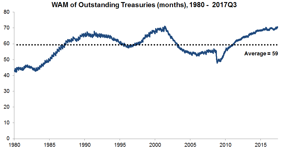
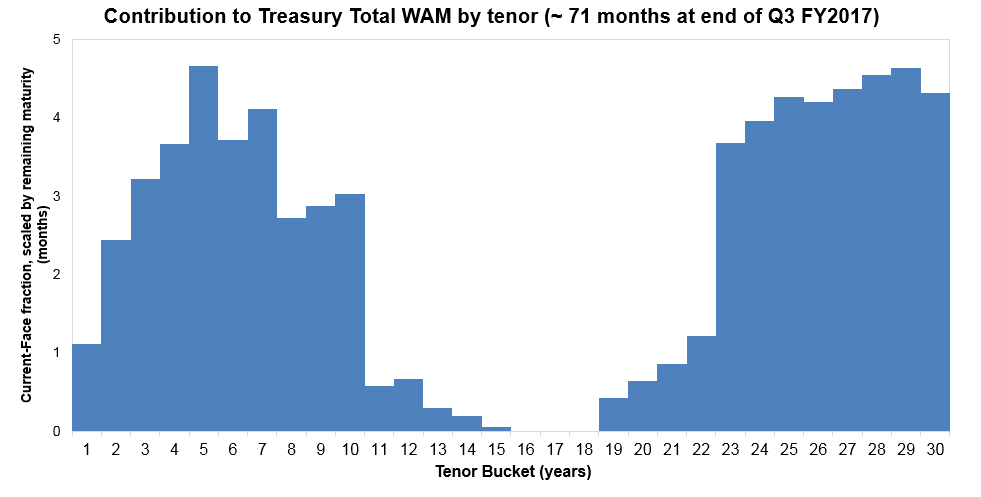
It is true that the WAM of a portfolio can serve as useful and intuitive shorthand for both its cost and risk implications over time. The quantity is straightforward, transparently model-free for anyone to compute, and can be done so using public data. Yet all recognize that it has inherent shortcomings. For example, a ”barbelled” portfolio composed of half $1$-day and half $30$-year bonds has essentially the same WAM as a portfolio containing only $15$-year bonds, but very different rollover and risk implications. (In this extreme example, half of the former portfolio will need to be refinanced in one day.) Similarly, the WAM of the US Treasury portfolio, which is at or near modern-day highs (see Figure 1), largely reflects increased issuance flow (in both size and frequency) of longer-dated borrowing (7- and 10-year notes, and 30-year bonds) that began near the beginning of this decade. The resulting WAM of around 70 months is a consequence of disproportionately adding these longer-dated bonds to the portfolio (closely following the 2001-2006 discontinuation of 30-year issues), which can be seen to have a marked ”hole” near maturities of around 15 to 20 years. (See Figure 2.)

Figure 1: WAM (weighted-average maturity) of Treasuries outstanding, including those held by the Federal Reserve. The current (2017Q3) WAM of roughly 71 months is near modern historical highs.

Figure 2: An illustration of the distribution of outstanding Treasury securities, as regards their contribution to WAM. Here the current-face of each security is scaled by its remaining maturity (in months) and divided by the total size of the portfolio; the resulting quantities, having units of months, are then aggregated by maturity bucket. The sum of the column heights in the chart is the WAM itself. This visualization illustrates that the Treasury portfolio is essentially bifurcated into two distinct portfolios rather than uniformly allocated. The shorter ($\leq 15$ years) portion of the portfolio has a WAM of around $33$ months, but the longer ($20+$ years) portion of the portfolio serves to boost WAM to its elevated level (approximately 71 months). All quantities as of end Q3 FY2017.

But WAM masks the fine-grained details of a maturity profile, and to discuss debt management in terms of managing the portfolio WAM leads to oversimplification of what is in reality a dynamic, evolving process that is highly influenced by historical issuance patterns.

An added, less well appreciated observation is that WAM is a stock measure (describing, after all, the outstanding portfolio). Although such a proxy does fit with a rich literature in sovereign debt issuance modeling that addresses the optimal distribution of stock, in practice Treasury debt management choices and decisions (absent a significant buyback program) have a more direct effect not on stock but on flow. That is, under current policy it is (largely) the makeup and sizing of the regular, ongoing supply of new issuance that is under the direct control of the US Treasury. This mismatch, between control variables and ostensible target metrics, can make certain statements and concepts phrased in terms of WAM misleading.

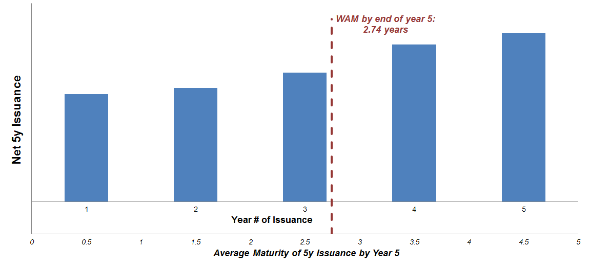
For example, consider a hypothetical strategy of using only 5-year issuance: this might sometimes be interpreted and spoken of (loosely) as using a ”5 year WAM” strategy. But regular, periodic issuance of 5-year debt does not create a portfolio with a 5-year WAM (the actual WAM of the resulting portfolio would likely range between 2.5-3 years, and fluctuate with deficits). See Figure 3 for an illustration, which shows why this occurs and why there is a meaningful difference between the maturity of new-issuance and the WAM of the resulting portfolio. It also illustrates that considering and managing the maturity of new debt does not necessarily result in a predictable WAM, which can and will be affected by fluctuations in deficits and rates. (Conversely, managing to a particular WAM would require allowing new issuance to fluctuate with deficits and rates.)

As of 2017, the Treasury portfolio has a WAM of almost 6 years (far longer than 3), issues at an average maturity of around 3.5-4 years (shorter than 5) and with a median maturity that is even shorter, at around 3 years. How then to translate a statement about something as simple as all-5-year issuance into the language of WAM? How to interpret its implications, or even speak about new-issuance allocation at all, when it is WAM that is the lingua franca of debt management? Managing debt flow but measuring and tracking WAM becomes a regular source of miscommunication.

Figure 3: Example of a hypothetical portfolio created by issuing only 5y debt yearly, spread throughout each year, in the face of rising and randomly-fluctuating deficits. The average maturity of a series of 5y notes with the same size spread over five years would be 2.5 years, but because deficits grow and fluctuate, the actual WAM of such a portfolio would fluctuate too, and likely be in the 2.5-3 year range.

The truth is that despite these drawbacks, and however aware debt managers are of them and attempt to move beyond undue focus on WAM, its simplicity and ubiquity – and, importantly, the lack of alternatives – makes it “too useful” not to revert to as a strategy metric and shorthand, a common reference point for communicating strategy.

2.2 Flow and the cost-risk tradeoff

As stated above, this piece describes an effort undertaken to improve this situation by summarizing and visualizing Treasury issuance in a way that, while it preserves much of the simplicity and transparency advantages of WAM, is more aligned with the dynamic and flow-centered nature of practical debt management and its tradeoffs. We do this by associating to any given issuance pattern or set of sizes two proxy metrics, one abstractly corresponding to cost and the other to risk. An issuance strategy or pattern is thereby represented as a point in a cost-versus-risk space (i.e., risk-return but from the issuer perspective). As patterns change or issue sizes are adjusted, the implied cost-risk tradeoff changes. By plotting the trajectory over time, one can illustrate the path of Treasury debt management either historically, or in a given projected scenario. The resulting graph in cost-versus-risk space allows for visualization of debt-management strategy directions and movements in a way that harnesses intuitions and stylized facts from classical portfolio theory and efficient frontiers.

Often, scenario analysis in Treasury debt management involves charting out and considering a future path of issue-sizes over a planning period (for example, $10$ years). With over $250$ auctions per year, in the most general of such constructs there would be at least $2500$ independent control variables to consider. Simplification is inevitable. But even if planned representative issue-sizes in a forward planning period are (for example) stipulated to be constant yearly, with $14$ security types this still creates $140$ independent variables. Further reduction of the dimension of this problem is necessary to comprehensible scenario analysis or consideration of the impacts of a particular issuance strategy shift.

Practically speaking, then, scenario analysis largely confines itself to consideration of high-level, easily-comprehended strategy directions. To illustrate, suppose projected funding requirements compel Treasury to increase borrowing patterns versus status quo. Various groupings of instruments, and/or tenor categories, may be considered, such as: increasing bill sizes pro rata, increase coupon-bond sizes pro rata, twist short (so that short-tenor instrument sizes are increased faster than for long tenors), twist long, ”barbell” (e.g. increase the very short and very long tenors, against the medium tenors), and so forth. The time dimension involved in forward planning only complicates matters, because (unlike with, say, equity allocation) the question is not how to allocate ”right now” but how to do so over time. And allocation is dynamic; it can and does change over time.

2.3 Why focus on steady-state?

It may be objected that a steady-state debt distribution equilibrium is unconvincing or unrealistic as a model of debt dynamics. It might fairly be expected that shocks, feedbacks, endogenous prices, and/or other more complex dynamics than are captured in this framework are what largely drive this or that salient conclusion to be drawn from more thorough and complex approaches to modeling debt issuance (we are agnostic, but admit to being unconvinced in that regard). While such critics are correct that this framework is (unabashedly) a simplification, we hasten to add that our claims for the usefulness of such an approach are modest, and not tightly bound to any particular strong assertion about whether steady-state has been or will be, in fact, attained. As stated above, an immediate goal is simply to develop a way of understanding and communicating intuitions about debt-dynamics, as they arise in planning, simulation, or modeling of debt issuance. To the extent those dynamics are driven at least in part – perhaps in large part – by the underlying mechanics of the evolution equations investigated below, surely one can only benefit from actually exploring and understanding the consequences of those equations, simplification though they are, to the full extent possible.

In addition, we observe that there appear to be certain characteristics shared by a large class of debt issuance models that readily and immediately motivate investigation in this direction. Consider models such as those developed in [6] or [19]. What is, in fact, going in on such models? A rolling debt portfolio, under conditions of a well-defined prescribed issuance strategy, is simulated periodwise up to a large time horizon (say 20 or 30 years). The simulations are driven by an ensemble of input-paths (of interest rates, output gaps, deficits, and so on) drawn, implicitly, from a stochastic distribution calibrated against a history of economic conditions and constructed or constrained so as to be, it is believed, economically feasible. Metrics representing e.g. cost and risk are then observed in each simulation at or approaching the simulation horizon, and averaged over the ensemble of realizations. Finally, conclusions are drawn regarding the relationship between these long-term metrics (as estimated by the numerical simulation and averaging process) and the assumed issuance strategy, to derive conclusions or relationships regarding efficient or optimal policy directions.

Mathematically, a model of this type can be thought of as a Monte Carlo simulation: a numerical estimation of the (perhaps incalculable analytically, but theoretically exact) mapping from the space of issuance strategies to the chosen metrics (i.e. distributional means or other moments of portfolio observables under the stochastic distribution of the input paths) at the long-time horizon chosen. This paper considers nothing other than the consequences of such a mapping as that long-time horizon, which after all is arbitrary, tends to infinity. Moreover, in most such models we have encountered, as can often be seen from their fan charts, the stochastic input paths driving simulations are quickly mean-reverting (e.g. Gaussian) to some apparently steady average, and not especially skewed, distribution, with little apparent influence from initial conditions. Note that the basic yearly budgeting equation governing debt dynamics, as usually expressed, is linear. All of this only buttresses the notion that the theoretical long-term steady-state of such a simulation is, to a significant degree, what is actually being approximated in such a simulation, and that the average metrics thus compiled are approximations to or at least well-proxied by the exact analytical metrics arising in a steady-state. (Indeed, were the closed-form steady-state formulas developed below unknown, a perfectly legitimate way to approximate them would be to run an ensemble of debt-simulations under steady or an ensemble of quickly-mean-reverting input paths and measure mean in-simulation observables at some large time-horizon.)

What follows then can be conceived of as an alternative approach to modeling or scenario analysis of the types referenced above, and one that attempts to capture the salient features and expected long-term dynamics of more complex quantitative models (e.g. Monte Carlo methods that, in principle, estimate or at least approach a steady-state portfolio given market and strategy assumptions) that are, unavoidably, several orders of magnitude more computationally intensive. It is also a goal to obviate the need to focus on specific dollar issue sizes and near-term fluctuations along finely-calibrated forward market paths, and instead bring relative allocation, borrowing fractions, and underlying dynamics to the forefront of strategic consideration.

Alternatively, and less ambitiously, this piece merely presents simple cost and risk proxy metrics relevant to and useful in visualizing issuance strategy, in the context of and as an adjunct to what is, in the abstract, a complex optimal stochastic control problem (for examples of the latter we can refer the reader to e.g. [6], [11], [13]). Note these metrics and formulas are substantively identical to those presented and discussed, with a slightly different emphasis, for the zero-debt-growth case in [9]. Equivalent formulas have also been more recently used to aid discussion of modeling results by the Treasury Borrowing Advisory Committee in their presentations to Treasury, see for example PDF p. 68 of  [20] or p. 112-113 of  [21].

The next section gives definitions necessary to understanding of the proxy metrics we put forth.

3 Definitions

This section describes definitions and mathematical constructs required for the metrics we introduce. The starting point is the government’s periodwise budget equation, which (aside from, possibly, notation) is standard and does not depart from e.g. [3].

Time is discretized into periods, which we will take to be (fiscal) years. In each year $t=0,1,2,\dots$, dollar outlays are made from the Treasury General Account (TGA) broadly owing to three sources:

• The difference (a deficit, $D_{t}$) between fiscal spending and tax receipts. (This may or may not coincide with ”primary deficit”, as it includes all (non-interest) spending items that may necessitate debt financing including e.g. student loans.)

• Interest payments on debt, $I_{t}$

• Repayment of maturing debt principal, $M_{t}$

To ensure that these outlays do not add to the money stock (a phenomenon that would register as a reduction in the TGA balance) they must be offset by dollar inflows. This is achieved by issuing new debt in an amount $N_{t}$ sufficient to generate the required cash proceeds. Assume for simplicity that the TGA balance is held constant year over year. We therefore must have

$$N_{t}=D_{t}+I_{t}+M_{t}$$ (3.1)

where $N_{t}$ is the face notional amount to be issued in year $t$. (Here issuance is assumed to be at par; any issuance discount is assumed to be contained in $I_{t}$.) More generally, the case where the TGA balance is not constant but rises over time could be addressed, by (for example) including cash-balance changes into the deficit term $D_{t}$; as long as cash-balance grows at a rate no faster than do deficits, the below analysis is unaffected.

Assume all debt can be issued in one of several tenors $j\in(1,2,\dots,T)$. Note here all Treasury bills are to be lumped into the $j=1$ bucket; for simplicity the interest on 1-year debt in year $t$ is assumed due in year $t+1$. (As well, the inflation component of TIPS and the floating coupons of FRNs are ignored in this construct; where necessary they are lumped in with their nominal counterparts by tenor.)

For our purposes here, an issuance strategy is assumed to consist of selecting constant fractions $f_{j}$ a priori that govern how much of each tenor to issue. That is, in year $t$ Treasury will issue at tenor $j$ the amount

$$N_{t,j}=f_{j}N_{t}=f_{j}(D_{t}+I_{t}+M_{t})$$ (3.2)

Obviously the assumption that real-world issuance strategy is described by a set of flow fractions is debatable. In practice, modern Treasury issuance practice has historically been stated and managed in terms of the auction sizes (in nominal dollar terms) of its regular notes and bonds. When necessary, changes to those sizes may be considered going forward. The resulting issuance process has, consequently, often been characterized by punctuated periods during which nominal sizes (and not issuance-fractions) of tenors have remained steady, unless and until changed. This is done in a deliberate manner in keeping with Treasury’s philosophy of ”regular and predictable” issuance. Clearly, the (empirical) issuance fractions that result from such a process need not be (and have not been, historically) constant or steady. However, it will be seen that as an approximation to the actual process over long periods, and as a description of the stance of issuance allocation (as regards its long-term implications), this fractional model will suffice for our purposes.

Because $I_{t}$ and $M_{t}$ depend on $N_{s,j}$ for $s\geq t-T$, equation 3.1 is a $T$-period recursive difference equation for the yearly vectors of new-issue sizes $(N_{t,j})_{j=1}^{T}$, in which deficits $D_{t}$ play the role of an exogenous forcing term, one that is presumably unrelated to debt management policy as such.

One gauge of the cost of this issuance strategy is just its new-issue weighted average maturity (NWAM); if measured in years, this quantity can be immediately read off of the issuance fractions $f_{j}$ via the formula

$$NWAM=\sum(j-\frac{1}{2})f_{j}=\sum jf_{j}-\frac{1}{2}$$

(The $1/2$ term here adjusts for the fact that Treasury issuance is typically spread throughout a year.)

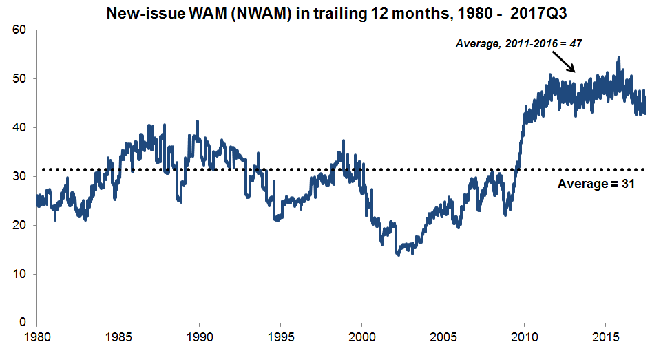
In a sense this is the flow equivalent of WAM. This metric itself can provide useful insights into debt management policy. For example, during the period 2010-16 Treasury WAM steadily increased, which has been characterized as a policy of ”actively” increasing WAM. But it may be more descriptive to say merely that Treasury used a very stable and unchanging new-issuance pattern, and that pattern had a longer-tenor bias. This is illustrated by the relatively flat NWAM throughout the period. (See Figure 4.) The reason WAM increased as a result is that the issuance pattern Treasury set in place in 2010-11, and then left largely unchanged, was long-biased (had a high NWAM of 45-50 months) compared to historical practice and to the (lower) breakeven NWAM that would have maintained the length of the outstanding portfolio at its then-extant level.

Figure 4: NWAM (new-issue weighted-average maturity) of Treasury issuance in trailing 12 months. Since 2010-11 the average maturity of new-issuance has been well above historical averages.

4 Steady asymptotic limit

How is the recursion (3.2) used to derive cost and risk proxies? What we seek is to characterize the long-term implications of using a given strategy, as described by the issuance fractions $f_{j}$. Conceptually, we would like to think of the portfolio as being in (in some sense) a ”steady-state”, so that we may ask questions about how current issuance affects or causes the portfolio to drift toward that steady-state. This long-term, steady-state-centered point of view is meant to be the logical extension of a common modeling approach in which a portfolio, under some issuance strategy assumption, is simulated for a long period of time (10, 20 years or more) and then the resulting metrics are averaged and examined at the horizon or in an abstract future period (cf. [6]).

Granted, it is not obvious that such a steady-state can or does exist. In practice, fiscal deficits and interest rates fluctuate in a correlated and possibly secular manner; issuance tenors and strategies, meanwhile, can change. The Treasury portfolio historically shows little signs of ever having converged to a steady-state per se. As well, nominal quantities all grow over time, restricting the possible quantities that can even be said to be steady or homogeneities that may exist. A model with the ambition of calculating and describing the ”steady-state”, long-term consequence of an issuance strategy evidently must be abstract and hypothetical in nature. Simplifying assumptions must be made.

Here, we make two major assumptions:

• Deficits grow geometrically at a constant rate of $g$ per year ($D_{t}\sim(1+g)^{t}$).

• The yield curve (interest rates $r_{j},j=1,\dots,T$) is static and constant yearly.

The reader will object that the above are unrealistically simplified assumptions; they are better conceived of as representing long-term averages around which a real market-data path might plausibly fluctuate and to which it might mean-revert.

The motivation for these assumptions is precisely that these appear to be the conditions necessary for a rolling Treasury portfolio to become self-similar and approach a meaningful ”steady-state” as $t\to\infty$. Indeed, under these assumptions we can solve for the long-term asymptotic equilibrium portfolio of equation (3.2) and observe its properties and metrics. In the below, we highlight two such metrics that naturally represent this asymptotic steady-state portfolio as regards its cost and risk.

4.1 Cost proxy

Under appropriate and historically plausible conditions on $r$ and $g$, we show in Appendix A.2 that the effective interest-cost percentage, or (to abuse terminology slightly, given our approximation of discount bills as 1-period coupon bonds) weighted-average coupon (WAC) of the portfolio under the strategy $f$ (defined as $WAC_{t}=I_{t}/z_{t-1}$, where $z_{\cdot}$ represents the total debt stock) approaches a constant asymptotic limit

$$WAC_{t}\to WAC^{*}=\sum w_{j}r_{j}$$

where $w_{j}$ are weights that depend only on $f$ and $g$ (not on $r$):

$$w_{j}=\begin{cases}\cfrac{f_{j}(1-(1+g)^{-j})}{\sum_{k}f_{k}(1-(1+g)^{-k})},&g>0\\ \cfrac{jf_{j}}{\sum kf_{k}},&g=0\end{cases}$$ (4.1)

In essence $w_{j}$ are compounded and growth-adjusted new-issue fractions. They represent the implication that using issuance strategy $f$ has for interest cost – how using allocation $f$, in effect, ”samples the yield curve” in the long haul.

The weights $w_{j}$ are adjustments of the new-issue fractions $f_{j}$. Note that for $g>0$ the adjustment (downward) is larger for short tenors than for longer tenors. This reflects the fact that longer-tenor interest rates play a larger role in portfolio WAC when the portfolio is dominated by recent issuance and (consequently) recently-issued longer bonds are present as a significant component of stock. That is precisely the situation when deficit growth $g$ is positive and large: recent issuance is more prominent.

The quantity $WAC^{*}=WAC^{*}(f;g,r)$ serves as a cost indicator of using issuance strategy $f$. Obviously it is not intended as a true calculation of the cost either ”right now” or on any particular path; rather, it is a gauge of the expected long-term, structural cost (asymptotically) if the strategy is to be maintained, and if near-term fluctuations in deficits and rates are neglected. But given that Treasury subscribes to a philosophy of ”regular and predictable” issuance, and does not attempt to time the market, in our view it is the precisely this long-term asymptotic expectation that is the proper orientation when it comes to a high-level cost assessment.

Of course, $WAC^{*}$ also depends strongly on the particular asymptotic rate assumption $r$. To remove this dependence, we calculate a quantity representing a ”WAC-effective” tenor:

$$t_{WAC}=\sum jw_{j}$$

Higher/lower values of $t_{WAC}$ should be associated with higher/lower cost, all else equal (and assuming an upward-sloping and relatively-smooth yield curve $r$). This makes $t_{WAC}$ – which is effectively a variant of NWAM, but using compounded and growth-adjusted weights $w$ rather than the issuance fractions $f$ – a useful rate-assumption-free cost proxy for issuance strategy $f$.

4.2 Risk proxy

Opinions and choices vary on how to gauge risk in debt-management. One can find in regular use as risk metrics the stochastic variance (i.e. uncertainty, whether conditional or unconditional) of interest-cost, the variability of interest-cost one can expect to observe unfolding over time, and measures of interest cost such as Cost-at-Risk ($CaR$) and variants that are based on the tails of the distribution of outcomes (examples for some/all of these can be found in, for example, [1], [2], [6], [7], [8], [12], [13], [14], [19]). There is also a growing view that the focus of cost quantification ought to be the primary balance (or total deficit) rather than interest cost in isolation (cf. [4], [17], [19]). Some sovereigns also place exogenous bounds on simple gross quantities such as required auction sizes, gross interest cost, or $Debt/GDP$; these too, where applicable, serve as risk constraints.

Without taking specific a view on the matter, we simply observe that arguably, any/all of these are dependent on and correlated with a simple quantity, the yearly maturing amount (i.e., rollover fraction). After all, the higher a percentage of the portfolio that must be rolled yearly,

• The more exposed is the portfolio to unanticipated interest-rate movement;

• The more volatile we can expect the portfolio interest cost to be (locked-in interest costs are, by nature, not volatile over time);

• The larger tail measures such as Cost-at-Risk should be (again because the portfolio is more exposed to unanticipated spikes in interest rates, to tails in their distribution);

• The larger the bill issue sizes are (more bills is part and parcel of what creates high rollover).

The yearly rollover amount is therefore a simple and useful risk proxy. It is calculable in the asymptotic steady-state setup described above. This quantity $RR_{t}$, representing the percent of portfolio in year $t$ that matures by $t+1$, is shown in Appendix A.3 to approach a constant limit:

$$RR_{t}\to RR^{*}=\sum\tau_{j}w_{j}$$

where the weights $w_{j}$ are as defined in (4.1), and

$$\tau_{j}=\begin{cases}\cfrac{g}{(1+g)^{j}-1},&g>0\\ \cfrac{1}{j},&g=0\end{cases}$$

As with $WAC^{*}$, the measure $RR^{*}=RR^{*}(f;g)$ gauges the long-term, asymptotic, steady-state implication of using issuance strategy $f$, but for risk. Namely, using $f$ indefinitely can be expected to create a portfolio of which the fraction $RR^{*}$ must be rolled yearly. Higher $RR^{*}$ indicates higher risk; this is our risk proxy metric.

4.3 Frontier

A natural question at this point is which strategies comprise the efficient frontier under these cost and risk metrics. In Appendix A.4 we show that under certain regularity conditions on $r$, when the required risk level is fixed at some given level $\tau_{j}$ (i.e. the constraint $RR^{*}\leq R$ is imposed for $R:=\tau_{j}$), the strategy that minimizes the cost measure $t_{WAC}$ is issuance concentrated on the single tenor

$$j:=j^{*}(R)=\begin{cases}\cfrac{\log(1+\cfrac{g}{R})}{\log(1+g)},&g>0\\ \cfrac{1}{R},&g=0\end{cases}$$

When $R$ is not of the form $\tau_{j}$ for integer $j$, but lies in between $\tau_{j}$ and $\tau_{j+1}$, then the lowest-cost strategy is an appropriate blend of issuance at tenors $j$ and $j+1$. So in effect, for any level of risk $R$ these metrics imply there is a ”sweet spot” tenor given by the formula $j^{*}(R)$ around which a concentrated-issuance strategy is the cost-dominant one for risk $=R$. This tenor is illustrated in Figure 5 for several choices of $g$.

Figure 5: ”Sweet-spot” tenor vs. rollover ($RR^{*}$) constraint. Single-issuance strategy at the given tenor (or if not possible, a blend of nearby tenors) dominates other issuance strategies $f$ with the same $RR^{*}(f)$. Frontier is shown for $g=0,4,8,12\%$; higher values of $g$ reduce the risk-mitigation created by longer-tenor issuance, because faster deficit-growth reduces the relative importance of long-past issuance to the portfolio, making shorter tenors more efficient.

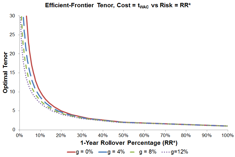
Note in the limit as $g\to 0$ this optimal tenor is simply $j=1/R$ (see solid curve in Figure 5). Stated conversely, when $g=0$ the ”risk” of $j$-year issuance using our metric is just $RR^{*}(g=0)=1/j$, recovering the intuitive notion that a $j$-year issuance strategy creates a portfolio of which roughly $1/j$ is rolled yearly. Indeed, [18] proposes a risk proxy based on assigning weight $1/j$ to $j-$period borrowing. By using the metric $RR^{*}$ as risk proxy, we are able to make the appropriate and growth-adjusted generalization of that simple intuition to arbitrary new-issuance strategies $f$.

5 Long-term deficit and rate assumptions

The metrics described above depend on deficit-growth and interest rate assumption parameters. For our purposes it is best to calibrate these to longer-term averages that can serve as a plausible description of asymptotic behavior.

For rates we can use, for example, a simple average of history rates (see Table 1). Such a yield curve is wider than the current market environment as of 2017, so it embeds an assumption that some reversion to the mean or normalizing will have taken place in the long-term. Internal calculations use a set of long-term forward rate assumptions produced by OMB as part of its budget process.

Table 1: Historically averaged yields 1981-present (derived from H15 curve; source: FRED).

Tenor	1y	2y	3y	5y	7y	10y	20y	30y
Yield (%)	3.24	3.56	3.79	4.22	4.54	4.79	4.88	5.39

For deficits we observe the log-linear trend of deficit growth over several historical decades (post-1970, when primary deficits began to be the norm) to be roughly $g=8\%$, so that is our base case choice. See Figure 6.

Figure 6: Primary deficits (source: FRED) portrayed log-linearly, excluding surplus years. The long-term trend (post-1970) is closest to an $8\%$ per year increase. The implied growth of future primary deficits and other-means-of-financing forecast by CBO (also shown) as of June 2017 is consistent with this trend.

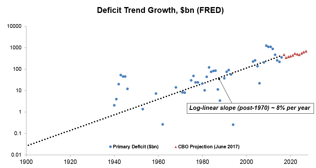
Because the intent is to be parsimonious and represent average dynamics rather than to overfit to any particular rate or deficit scenario, the hope is that results are not overly sensitive to these choices. A natural question therefore is how our proxy metrics vary with the rate and deficit assumptions behind them. Obviously $t_{WAC}$ is unaffected by the particular choice of $r$, by design. $WAC^{*}=\sum w_{j}r_{j}$ depends in a linear way on $r$; tilting $r$ wider and steeper would increase $WAC^{*}$ (and conversely for tighter/flatter), but in a somewhat uniform way. That is, when comparing two strategies in terms of $WAC^{*}$, simple shifts or rescalings of $r$ (within plausible limits) will tend not to materially alter the relative cost relationship between them.

The effect of the deficit growth assumption $g=8\%$ may appear more ambiguous. Generally, for a given strategy $f$, increasing the assumed $g$ will increase its computed cost ($t_{WAC}$) but decrease its computed risk ($RR^{*}$). Figure 5 shows the effect of these shifts for various choices of $g$ on frontier (concentrated-issuance) strategies. As with rates, such a shift in $g$ within a plausible range of $4-12\%$ appears unlikely to materially alter conclusions drawn regarding the relative cost/risk relationship between two sufficiently-distinct strategies.

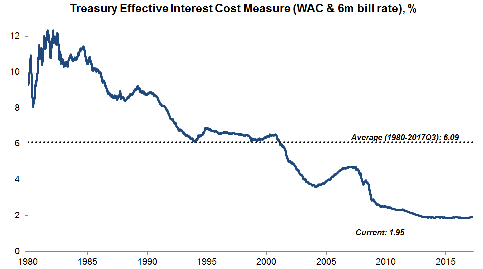
As stated in Appendix A.1, there is also a technical requirement, for our simple construction to lead to the explicit analytical formulas described above, that $g>WAC^{*}$. (Otherwise the equilibrium $WAC^{*}$ can only be calculated implicitly.) This does not appear to be overly restrictive; as shown in Figure 7, using a simple estimate of the effective WAC (adjusting the WAC of coupon-bearing securities by the $6m$ bill yield $\times$ the bill fraction of the portfolio) we see that only in the early 1980s Volcker era did the effective-WAC exceed $8\%$. (Note, this was also a period when deficit growth was far higher than $8\%$ per year.) The average is closer to $6\%$ and the recent trend has been under $2\%$. All indications are that deficit-driven rather than interest-driven debt growth is the asymptotic behavior that is relevant.

Figure 7: Interest-cost measure based on weighted-average coupon (WAC) of outstanding Treasury securities, adjusted by the $6m$ bill rate $\times$ the bills percentage of the portfolio, from 1980 to 2017Q3. The adjustment is necessary because bills contribute a $0\%$ coupon to the naive WAC calculation.

It is also worth acknowledging that our calculations are in strict nominal terms and based on the simple mechanical mathematics of debt-rolling. In so doing we knowingly leave considerations such as the debt-to-GDP ratio and the intertemporal budget constraint, transversality conditions, and/or sustainability considerations (see, for example, [15]) aside. As well, apparently the oft-cited correlation or feedback between issuance, interest rates, and fiscal needs as in the tax-smoothing and Ramsey planning literature (cf. [16], [5], [10]) is omitted here.

6 Mapping strategy to cost-risk space

We have described how a set of issuance fractions $f$ can, under simple assumptions about deficits and rates, be mapped into cost-versus-risk space. There are several alternatives described above (depending on the level of exactness or abstraction desired):

• $f\to(RR^{*},NWAM)$

• $f\to(RR^{*},WAC^{*})$

• $f\to(RR^{*},t_{WAC})$

Summarize this abstractly by stipulating that to each set of fractions $f$ we form the mapping

$$f\to(R,C)$$

where $R$ is the risk-proxy metric and $C$ the cost-proxy chosen. (In what follows, unless otherwise stated we use $C=t_{WAC}$.)

To illustrate this mapping, when $f=e_{j}$ (i.e. concentrated regular issuance only at tenor $j$), this mapping becomes

$$f=e_{j}\to(\tau_{j},j)$$

The $j=1$ strategy maps to $(R=100\%,C=1)$, low cost but high risk. The $j=30$ strategy maps (with $g=8\%$) to $(R=0.88\%,C=30)$, high cost but low risk. Other examples of this mapping and its dependence on $g$ for single-tenor strategies $f=e_{j}$ are shown in Table 2, which also highlights the dependence on $g$, especially for longer tenors. (This also helps illustrate why we did not ignore deficit-growth in our construct, or use the naive rollover metric obtained by simply taking $\tau_{j}=1/j$.)

Note that in this reductive case, the choice of $r$ plays little meaningful role, as long as $r$ is monotone increasing (as would be the case for any plausible long-term asymptotic rate assumption). This is because using $C=WAC^{*}$ we just have $WAC^{*}=r_{j}$. Since $r_{j}$ is monotone-increasing in $j$, the two proxies are equivalent in the sense of sorting single-tenor strategies by relative cost (i.e., $r_{j}>r_{k}\iff j>k$ for all $j,k$).

Table 2: Examples of the mapping $f\to(R,C)$ where $f$ represents a single-tenor issuance strategy at tenor $j=1,2,3,5,7,10,30$. The cost proxy $C=t_{WAC}$ for this case reduces to $C=j$. (If $C=WAC^{*}$ is used instead, then we would just have $C=r_{j}$, which for monotone increasing rates $r$ would not alter the relative cost picture.) The risk proxy $R$ depends on the deficit-growth assumption $g$: faster deficit growth implies less relative rollover contribution from long-past issuance of longer tenors.

	Deficit growth factor (g)
Single-tenor strategy (y)	4%	8%	12%
1	(100%,1)	(100%,1)	(100%,1)
2	(49%,2)	(48.1%,2)	(47.2%,2)
3	(32%,3)	(30.8%,3)	(29.6%,3)
5	(18.5%,5)	(17%,5)	(15.7%,5)
7	(12.7%,7)	(11.2%,7)	(9.9%,7)
10	(8.3%,10)	(6.9%,10)	(5.7%,10)
30	(1.8%,30)	(0.9%,30)	(0.4%,30)

Real-world issuance strategies are of course not usually concentrated on single tenors, as for various reasons Treasury can be seen to issue regularly across the yield curve. But what this method allows is to place any nontrivial issuance pattern $f$ into $(R,C)$ space in a way that remains consistent with simple intuition about the tradeoffs between cost and risk in the single-tenor thought experiment. Applications of this principle are demonstrated in the next section.

7 Usage and results

In this section we describe how the proxy metrics described above are used to illustrate and visualize debt issuance strategy. All projected quantities are hypothetical and for illustrative purposes only.

7.1 Summarizing historical issuance strategy

How can these metrics, which by construction relate to asymptotic portfolio behavior, be applied to actual Treasury debt issuance? It can be observed historically that Treasury does not evidently select and then use indefinitely a single set of fractions $f$ for its issuance pattern. Instead, the issuance pattern can only be observed empirically, as a consequence of Treasury decisions and events. Nor does the asymptotic portfolio ever actually emerge, as fiscal, market and (indeed) debt management strategy may evolve and fluctuate.

But for historical issuance we can still analyze issue fractions a posteriori: aggregate all issuance within a fiscal year and observe the empirical issuance fractions that were used, by setting

$$f_{j}=A_{j}/A$$

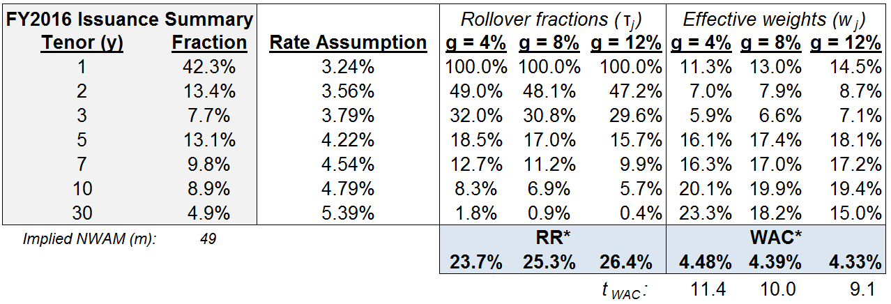
where here $A_{j}$ represents the amount issued in tenor bucket $j$, and $A$ represents total issuance, during the year. (Note that bills that were issued and matured prior to the end of the fiscal year are not counted in $A_{t}$, since it is meant to reflect net borrowing required to finance $D_{t}+I_{t}+M_{t}$.) Table 3 shows how this calculation applies to summarizing Treasury issuance during fiscal-year 2016.

Table 3: Fiscal-year 2016 Treasury issuance summarized as issuance fractions by tenor bucket. Bills are placed in the 1y bucket, TIPS/FRNs with their nominal counterparts. Bills issued/matured within the year are excluded; only net new issuance (live as of $9/30/16$) is included. Figures here exclude debt purchased by Federal Reserve SOMA account as auction add-ons, being not directly germane to Treasury issuance strategy.

Empirical Issuance Fractions (FY2016)
Tenor (y)	Security Type	Notional ($bn)	Flow	Issuance Fraction
1	Bills	$1,647	$1,647	42.3%
2	Notes/Bonds	$350	$520	13.4%
	FRN	$170
3	Notes/Bonds	$300	$300	7.7%
5	Notes/Bonds	$462	$509	13.1%
	TIPS	$47
7	Notes/Bonds	$381	$381	9.8%
10	Notes/Bonds	$267	$347	8.9%
	TIPS	$80
30	Notes/Bonds	$167	$189	4.9%
	TIPS	$22
	Total:	$3,892

We can thus create this mapping in each historical year $t$:

$$\mathrm{Debt\;issued\;in\;year\;}t\to f^{(t)}\to(R^{(t)},C^{(t)})$$

In so doing we are summarizing a year’s issuance pattern by mapping it to the asymptotic properties of the portfolio it would create if continued indefinitely. The table presented in Figure 8 summarizes this calculation when applied to 2016 issuance in fractional form.

Figure 8: Mapping $f\to(R,C)$ shown for FY2016 issuance summarized as empirical new-issue fractions, and using a long-term rate assumption derived from post-1980 historical-averages. Risk ($RR^{*}$) and Cost ($WAC^{*}$) proxies shown for three deficit growth assumptions, $g=4,8,12\%$. Using base-case $g=8\%$, the method summarizes 2016 issuance as having selected $(R,C)=(25.3\%,4.39\%)$ in cost-versus-risk space. Average new-issue maturity was around four years ($NWAM=49$ months), but $t_{WAC}=10$ implies that under this issuance pattern it is the $\sim$ 10-year interest rate behavior/assumption that will be of most importance to longer-term portfolio interest cost when issuing using this allocation.

Treasury issuance strategy from fiscal years 1981-2016 is summarized and portrayed in Figure 9 (using $g=8\%$) with this technique. The approach serves to highlight outlier years: 2015 was an especially long-biased issuance pattern; 2001-2002 were short-biased years (in large part due to the discontinuation of 30-year bond issuance).

Figure 9: Empirical Treasury issuance from FY1981-2016 summarized on a $(RR^{*},WAC^{*})$ diagram. Assumes deficit-growth trend $g=8\%$. Rate assumption derived from historical H15 rates, 1981-2016 (FRED). SOMA auction purchases and Bills issued as part of the Federal Reserve’s Supplementary Financing Program (SFP) are excluded for this exercise. Omits effect of the large-scale buyback operations in 2000-2002, which were largely focused on 15+ year debt, implying an effective issuance policy slightly shorter (higher $RR^{*}$) on net than portrayed here.

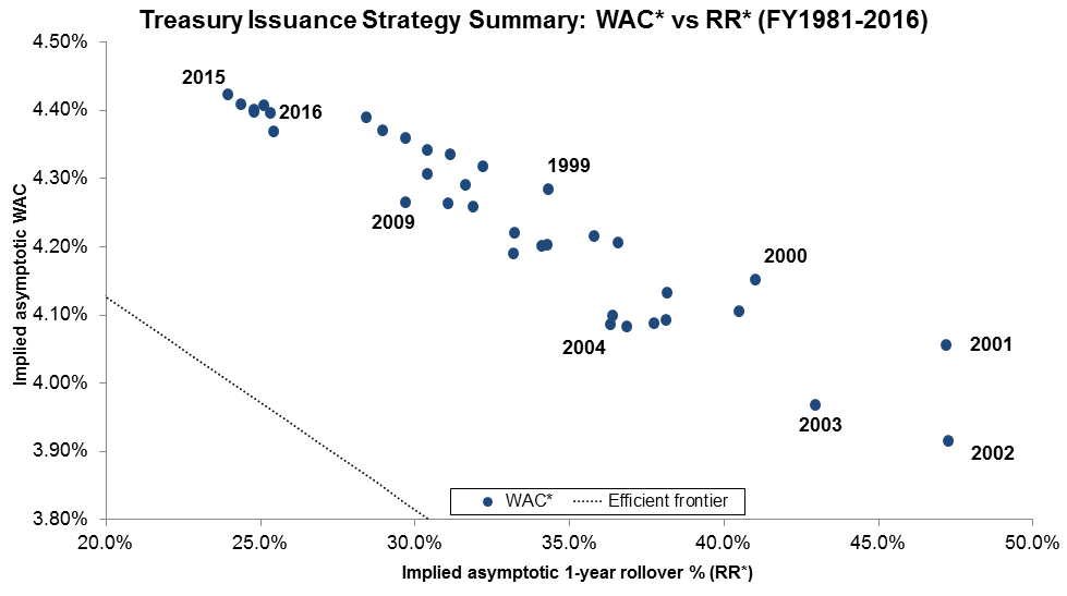
We see that current Treasury issuance (FY2016) has pulled back somewhat from its recent long bias. This is presumably a partial consequence of the mid-2015 decision to increase bills stock, but also of the February 2016 decision to reduce issue sizes of 5y and longer notes/bonds/TIPS.

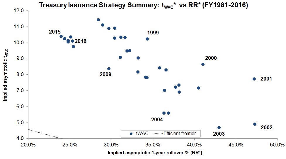
Figure 10 portrays the same diagram but using $t_{WAC}$ rather than $WAC^{*}$ as cost proxy. This transforms and stretches the diagram, but does not appear to materially alter the relative relationships between yearly strategies, or outliers. This should be unsurprising given the fact that $r$ is monotone-increasing (as would be any plausible long-term asymptotic interest-rate assumption).

Figure 10: Empirical Treasury issuance from FY1981-2016 summarized on a $(RR^{*},t_{WAC}^{*})$ diagram. Assumes deficit-growth trend $g=8\%$. The dependence of the cost metric on rates has been removed by using $t_{WAC}$ as cost proxy. Relative relationships between yearly strategies and outliers remain largely unchanged.

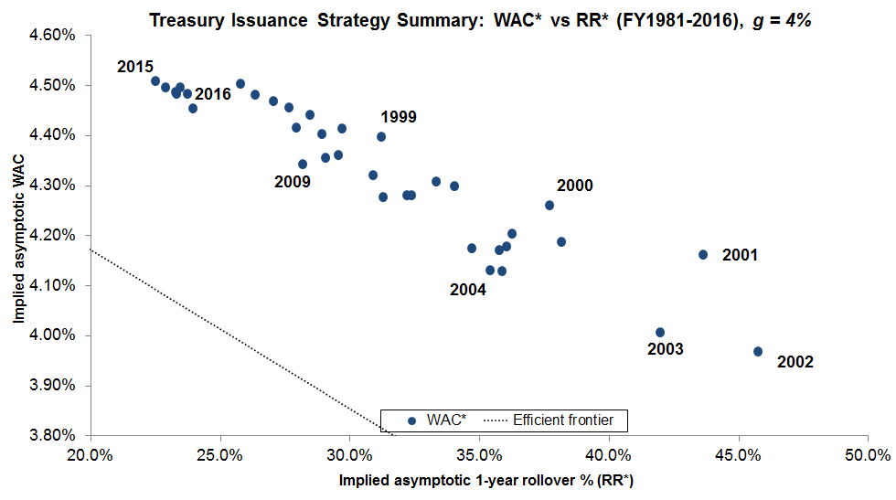
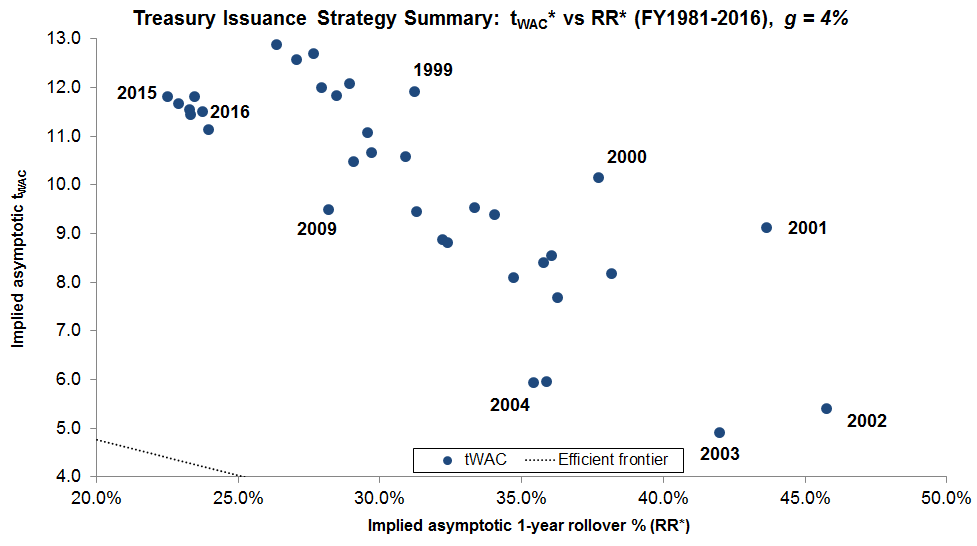
Figures 11-12 replicate these diagrams but using $g=4\%$ rather than $8\%$. We see that although the quantities change, relative relationships among yearly strategies are largely (albeit not entirely) robust to changes in the long-term deficit-growth assumption.

Figure 11: Empirical Treasury issuance from FY1981-2016 summarized on a $(RR^{*},WAC^{*})$ diagram, assuming deficit-growth trend $g=4\%$.

Figure 12: Empirical Treasury issuance from FY1981-2016 summarized on a $(RR^{*},t_{WAC}^{*})$ diagram, assuming deficit-growth trend $g=4\%$.

7.2 Spot issuance strategy

Rather than the a posteriori empirical analysis of the previous section, we can gauge the current stance of issuance strategy by using prevailing issuance sizes (rather than rolled-up issuance throughout a year) to infer the new-issue fractions $f$ that they imply.

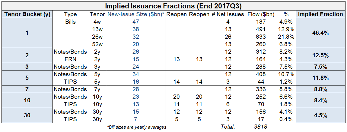
For example, the current size of a new-issue 30-year bond (as of 2017) is $\$15$ billion, a new CUSIP is issued four times per year, and each is reopened twice in amounts of $\$12$ billion. Under such a policy, the implied yearly flow of 30-year issuance is $4(15+12+12)=\$156$ billion. We calculate the flow for all other tenors in the same manner, and from those, the implied fractions $f$ these sizes represent. This is illustrated in Figure 13 for issuance sizes prevailing as of end Q3 2017. (As a technical note: when doing this for bills we use yearly-averaged bill sizes rather than current bill sizes, because bill issuance fluctuates throughout the year due to their role as fiscal shock-absorber. Since our goal is to infer the stance of issuance strategy we need to eliminate this exogenous seasonality effect.)

Figure 13: Treasury issuance strategy in terms of new-issue fractions inferred from new-issue sizes as of end 2017Q3. For bills, the average size over the preceding year is used in order to remove seasonality effects.

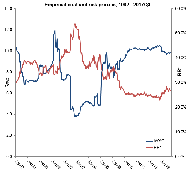
Spot strategies are calculated monthly in this manner from 1992-present (see Figure 14).

Figure 14: Implied monthly cost- and risk-proxies employed for Treasury issuance from 1992 - June 2017. Most-recent new issue sizes are combined with upcoming auction schedules to infer issuance fractions. CMBs, Bills issued as part of the Federal Reserve’s Supplementary Financing Program (SFP), and effect of 2000-2002 large scale buybacks are excluded for this exercise.

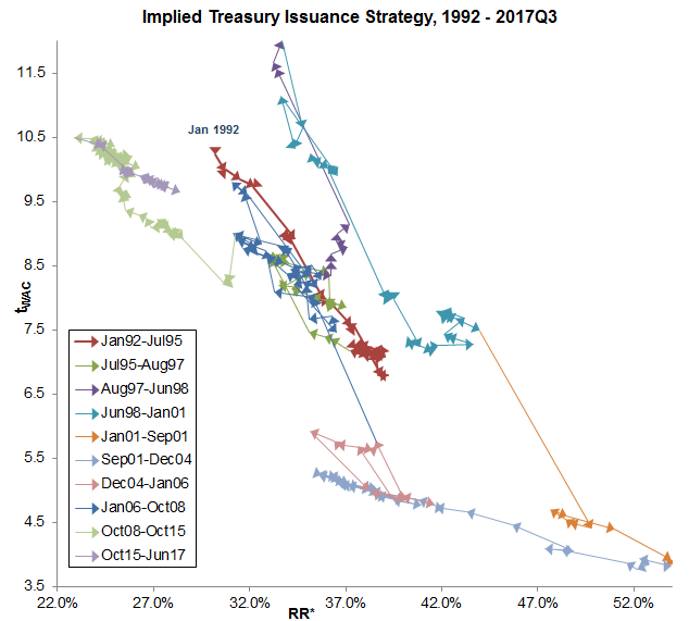
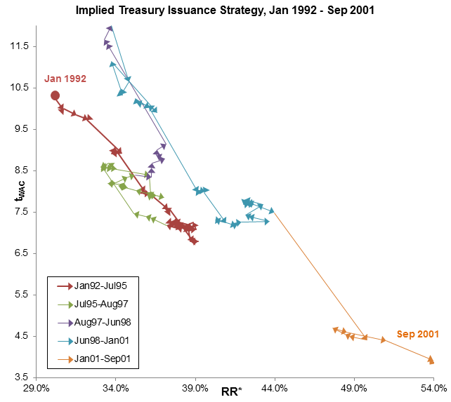
The joint evolution is portrayed in Figure 15 as a trajectory on an $(R,C)$ diagram. They are also broken out into individual periods in Figure 16. Several apparently distinct periods of Treasury issuance policy can be tracked on these illustrations:

• Reduced term borrowing from falling deficits in 1990s

• Elimination of 30y bond in 2001 - 2006

• Shift in term borrowing post 9/11/2001

• Lengthening of issuance allocation post-financial crisis

What is perhaps most salient here, in the final graph of Figure 16, is the clustering of policy points (green, upper left) that is seen from June 2010 - October 2015. This is the post-financial-crisis period of actively extending WAM, i.e., of employing a relatively static new issuance flow strategy with a long bias. The graph also shows that policy has begun to shorten modestly since, with the early 2016 reductions in all 5+ year issuance sizes.

Figure 15: Implied monthly path of Treasury issuance strategies from 1992 - June 2017 portrayed on an $(R,C)$ diagram. Most-recent new issue sizes are combined with upcoming auction schedules to infer issuance fractions. CMBs, Bills issued as part of the Federal Reserve’s Supplementary Financing Program (SFP), and effect of 2000-2002 large scale buybacks are excluded for this exercise.

Figure 16: Treasury Issuance strategy 1992 - 2017Q3 broken out into three periods: pre-9/11/2001, pre-financial crisis, and post crisis. 2010-2016 implied strategy shows as relatively constant (green cluster) in the third graph.

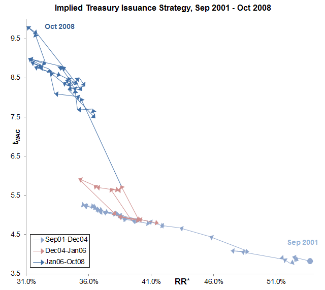
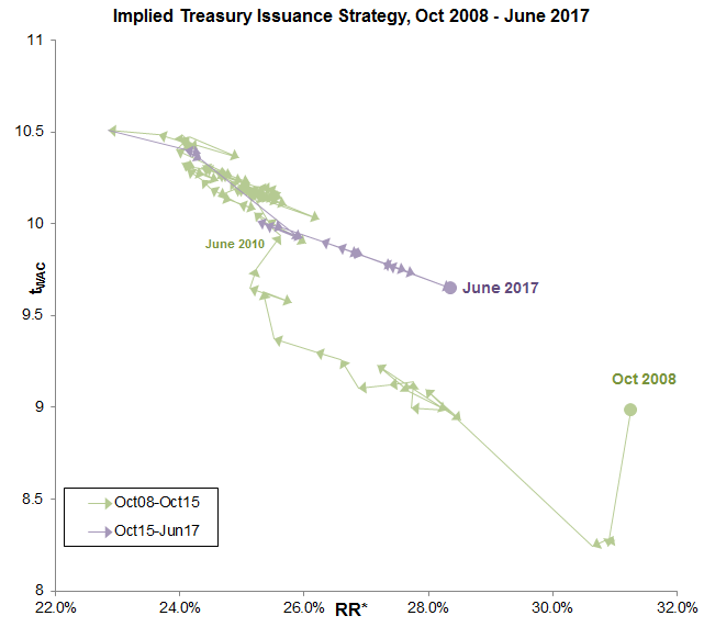
Applying $(R,C)$ metrics to spot-issuance patterns allows one to illustrate and visualize the path and direction of Treasury issuance in a way that lines up with how debt management is most directly announced and affected: by considering and/or making specific changes to issue sizes, by introducing or removing tenors, by changing auction schedules – by altering Treasury flow. Key historical decisions about Treasury issuance become plainly visible as movement in $(R,C)$ space. Conversely, periods such as 2011-16 in which (we assert) issuance strategy was effectively unchanged emerge as periods of little or no such movement. Note that in such periods of static issuance-strategy, WAM may be changing rapidly, which again highlights the distorted picture that can be painted by WAM.

7.3 Visualizing forward scenarios

Another benefit of mapping issuance to our representative $(R,C)$ metrics is that one can visualize the direction and effect of potential forward strategy options in a simple, intuitive way that escapes the need to examine dozens or hundreds of individual, projected future issue sizes.

For example, suppose financing needs are due to increase, and Treasury considers one of three strategy options in response:

• Increase only bill sizes incrementally as needed; leave all other sizes unchanged

• A shorter-tenor strategy preferentially favoring increases to bills, 2-3y notes, and the 2y floating rate note

• Keep bill, TIPS and FRN sizes constant, and increase the coupon stack pro rata as needed

In Figure 17 each of these three strategy approaches have been simulated for ten years under hypothetical rate and deficit assumptions, and the issue-size-implied allocations plotted as trajectories on the $(R,C)$ diagram. The different cost and risk implications of each of the strategy options become evident.

Figure 17: Yearly spot-$(R,C)$ diagrams of three hypothetical strategy approaches to financing incremental issuance over a 10-year forward period.

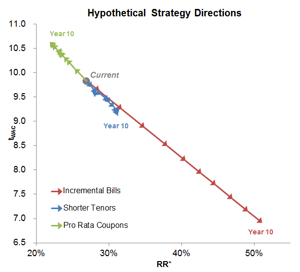
Portraying strategies in this way can help the policy maker understand the implications of and relationships between the cost-risk tradeoffs involved in strategy alternatives.

7.4 Constrained scenarios

The idealized efficient frontier mentioned above in $(R,C)$ space will typically consist of single-tenor issuance at some optimal tenor. Obviously this is not realistic, practical, or even desirable: Treasury has a long-established policy of issuing and maintaining many liquid benchmarks across the yield curve. There are other factors that can motivate against the literal interpretation of the concentrated issuance as optimal: the model omits feedback between issuances and rates, for example. For all intents, a concentrated issuance strategy $f=e_{j}$ would be considered inadmissible as a strategy option. This raises the point that strategies must belong to the admissible set of strategies in order to be legitimately considered as potential allocation adjustments.

Defining admissible strategies is ultimately the province of the debt manager; the process and considerations behind it are beyond the scope of this piece. But the effect of constraints – the debt manager’s ”policy window” of admissible strategies – on the analysis above, modifies the framework only slightly. A common approach may be to define lower and upper bounds $L$ and $U$ for the new-issuance allocations (or equivalently, upper bounds on changes from the current allocation $f_{curr}$); this defines the admissible set to be strategies such that $L\leq f\leq U$. Each such strategy has a point on the $(R,C)$ diagram, and it is straightforward to identify dominant directions that reduce cost or risk (see Appendix A.5). This idea is depicted in Figure 18.

Figure 18: Schematic illustration of issuance strategies constrained to a ”policy window” (admissible set) of allowed strategies, mapped to an $(R,C)$ diagram. Cost- and risk-dominant strategy directions from the current issuance pattern $f_{curr}$, as well as the optimal strategy within the admissible set (generally a simplex, for simple linear constraints), are easily calculated.

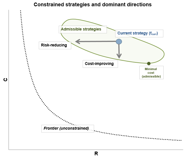
These dominant and constrained-optimal strategy directions could be used to inform policy decisions as to how to adjust borrowing patterns in the face of anticipated changes in financing requirements. For example, if deficits are anticipated to rise (creating a ”funding gap” if current issue-size flow were maintained), borrowing at which tenor(s) should be increased in order to close the gap? Different choices of tenor(s) imply different new-issue allocations $f$, which can be evaluated in terms of how they alter the cost and risk proxy metrics described above.

8 Summary

We introduce simple cost and risk proxy metrics that can be attached to empirical Treasury issuance, to ”spot” issuance patterns, and/or to forward issuance scenarios over time. These metrics are based on mapping issuance fractions to their long-term, asymptotic portfolio implications for cost ($C$) and risk ($R$) under mechanical debt-rolling dynamics, and given simple but necessary assumptions about asymptotic deficit growth and interest rates.

Mapping strategies to the resulting $(R,C)$ diagram enables one to harness the intuitions of standard portfolio theory, including the efficient frontier, which in this simple construct can be calculated analytically as an optimal single-tenor issuance strategy corresponding to a given risk tolerance.

Comparing historical or future issuance to the frontier and to past issuance enables policy makers to understand the direction and implication of the issuance decisions and implied tradeoffs they make in a way that is more dynamic and flow-centered than the traditional portfolio metric (WAM). As such these metrics are a valuable tool in discussing and understanding Treasury debt management.

Although the recursion model used to derive these metrics is clearly reductive, there is scope to expand on the work by, for example, endowing it with rate and deficit paths that are stochastic, mean-reverting, and correlated. Ultimately the steady $WAC^{*}$ and rollover-fraction $RR^{*}$ that we derive under our simple steady recursion model may be understood to represent – under appropriate assumptions – a special case of the stochastic equilibrium portfolio of a more complex and market-realistic model. Another potential area of refinement is to model the dynamics of inflation-linked (TIPS) and floating-rate (FRNs) debt rather than binning them with nominal counterparts.

While work is ongoing, we hasten to add that in bridging the gap between debt management modeling and practice model complexity and (often illusory) macroeconomic completeness ought not be impediments to intuitive metrics that can aid consideration and communication of debt management strategy – and, which are aligned with the considerations of debt management as it is implemented.

Appendix A Appendix

A.1 Equilibrium portfolio distribution

Start with equation (3.2) for new-issue amounts issued yearly, written as a vector equation for $n_{t}=(N_{t,j})_{j}$:

$$n_{t}=f(D_{t}+I_{t}+M_{t})$$

Define the stock in year $t$:

$$z_{t}=z_{t-1}+N_{t}-M_{t}=z_{t-1}+D_{t}+I_{t}$$

Using our asymptotic assumption about deficits we can write

$$D_{t}=D_{0}\gamma^{t-1}$$ (A.1)

where $\gamma:=1+g$.

We seek the steady average interest cost at equilibrium, defined as

$$WAC^{*}=\lim_{t}I_{t}/z_{t-1}$$ (A.2)

This means asymptotically we should have

$$z_{t}=\beta z_{t-1}+D_{0}\gamma^{t-1}$$

where $\beta:=1+WAC^{*}$. This can be solved:

$$z_{t}=z_{0}\beta^{t}+\frac{D_{0}}{\gamma-\beta}(\gamma^{t}-\beta^{t})$$

Now assume that $\gamma>\beta$ (i.e. that $g>WAC^{*}$). Under this assumption (which we acknowledge to depart from what is often assumed in the literature, cf. [3], but which appears to be the empirically relevant case), as $t\to\infty$ this becomes

$$z_{t}\sim\frac{D_{0}}{\gamma-\beta}\gamma^{t},$$ (A.3)

i.e. $z_{t}\sim O(\gamma^{t})$.

Define $q_{j,t}$ to be the stock of current tenor $j$ at time $t$. Of course, $z_{t}=\sum_{j}q_{j,t}$. Collect these quantities into a vector: $Q_{t}:=(q_{j,t})_{j}$. Stock of current-tenor $j$ comes from two sources: rolldown of current-tenor stock $j+1$ from the previous year, and new-issuance at tenor $j$ in the current year. This implies a recurrence for $Q_{t}$:

$$Q_{t}=SQ_{t-1}+f(D_{t}+I_{t}+M_{t})$$

where $S$ is a shift operator ($S_{ij}=\delta_{j,i+1}$). Notice that the maturing amount $M_{t}$ is simply

$$M_{t}=q_{1,t-1}=e_{1}^{T}Q_{t-1}$$

Therefore

$$Q_{t}=(S+fe_{1}^{T})Q_{t-1}+f(D_{t}+I_{t}):=RQ_{t-1}+f(D_{t}+I_{t})$$ (A.4)

where $R:=S+fe_{1}^{T}$.

We are interested in the evolution of portfolio fractions, defined as

$$\theta_{t}:=\frac{1}{z_{t}}Q_{t}$$

That is, $\theta_{j,t}$ represents the percentage of the portfolio at time $t$ with current-tenor $j$. From equation (A.4) we find

$$\theta_{t}=\frac{1}{z_{t}}Q_{t}=\frac{z_{t-1}}{z_{t}}(\frac{1}{z_{t-1}}Q_{t-1})+\frac{1}{z_{t}}f(D_{t}+I_{t})=\frac{z_{t-1}}{z_{t}}R\theta_{t-1}+\frac{1}{z_{t}}f(D_{t}+I_{t}):=A+B+C$$

and treat the terms $A$, $B$, and $C$ separately by using (A.3), (A.1) and (A.2) to write

$$A\to\frac{1}{\gamma}R\theta_{t-1}$$

$$B\to\frac{1}{\gamma}(\gamma-\beta)$$

$$C\to\frac{1}{\gamma}(\beta-1)$$

The equilibrium portfolio distribution $\theta_{t}\to\theta^{*}$ must therefore satisfy

$$\theta^{*}=\frac{1}{\gamma}R\theta^{*}+(1-\frac{1}{\gamma})f$$

or

$$\theta^{*}=(\gamma-1)(\gamma I-R)^{-1}f$$

Letting $y=\theta^{*}/(\gamma-1)$ we must have $(\gamma I-R)y=(\gamma I-S)y-y_{1}f=f$, or $y=(1+y_{1})(\gamma I-S)^{-1}f$. Equivalently

$$\theta^{*}\propto(\gamma I-S)^{-1}f:=T_{\gamma}f$$

where the constant of proportionality is pinned down by the condition that $\sum\theta^{*}_{j}=1$. So we may write

$$\theta^{*}=\frac{1}{||T_{\gamma}f||_{1}}T_{\gamma}f$$

and it is easy to show that $T_{\gamma}$ is an upper-triangular matrix with

$$(T_{\gamma})_{ij}=\frac{1}{\gamma^{j-i+1}},j\geq i$$

The preceding holds in the limiting case $\gamma\to 1$ as well.

A.2 Asymptotic WAC

Assume the interest-rate applicable to tenor-$j$ issuance in year $t$ is simply $r_{j}$. This is paid out in the following years $t+1,t+2,\dots t+j$ as an amount $r_{j}N_{j,s}$. Therefore the net interest owed in year $t$ from all prior-year issuance of tenors $j=1,\dots,M$ is

$$I_{t}=\sum_{j=1}^{M}\sum_{s=t-j}^{t-1}r_{j}N_{j,s}=\sum_{j=1}^{M}r_{j}f_{j}(\sum_{s=t-j}^{t-1}N_{s})$$

In the limit we seek, $I_{t}=WAC^{*}z_{t-1}=(\beta-1)z_{t-1}$, or

$$I_{t}\sim\frac{1}{\gamma}(\beta-1)z_{t}$$ (A.5)

using the asymptotic behavior (A.3) of $z_{t}$. To derive the appropriate $WAC^{*}$ rewrite the above as

$$I_{t}=(\sum_{j=1}^{M}r_{j}f_{j}b_{j,t})z_{t}$$ (A.6)

where

$$b_{j,t}:=\frac{1}{z_{t}}\sum_{s=t-j}^{t-1}N_{s}$$ (A.7)

Asymptotically, expression (3.2) for the sequence $N_{t}$ can be written

$$N_{t}=D_{0}\gamma^{t-1}+(\beta-1)\left[z_{0}\beta^{t}+\frac{D_{0}}{\gamma-\beta}(\gamma^{t}-\beta^{t})\right]+\sum_{j=1}^{M}f_{j}N_{t-j}$$

where we have symbolically inserted asymptotic expressions (A.1) and (A.2) for $D_{t}$ and $I_{t}$ respectively, and made use of the fact that the maturing amount relates to prior issuance by $M_{t}=\sum_{j=1}^{M}f_{j}N_{t-j}$.

This is a nonhomogeneous difference equation for $N_{t}$ of the form

$$N_{t}=\sum_{j=1}^{M}f_{j}N_{t-j}+a_{t}$$

where asymptotically, and using our assumption of $\gamma>\beta$,

$$a_{t}\sim D_{0}\gamma^{t-1}\frac{\gamma-1}{\gamma-\beta}.$$ (A.8)

It may be homogenized by defining $U_{t}:=N_{t}-Ca_{t}$, using

$$C:=\frac{1}{\sum_{j}f_{j}(1-\gamma^{-j})}$$

Then $U_{t}=\sum_{j=1}^{M}f_{j}U_{t-j}$; in particular, the sequence $U_{t}$ is bounded (because $\sum f_{j}=1$). As a result, $U_{t}/z_{t}\to 0$ as $t\to\infty$ and can be neglected. We are left with $0=N_{t}-Ca_{t}$ or $N_{t}\sim Ca_{t}$; returning to (A.7) we find asymptotically,

$$b_{j,t}\sim\frac{1}{z_{t}}C\sum_{s=t-j}^{t-1}a_{s}\sim C\frac{1-\gamma^{-j}}{\gamma},$$

where we have used expression A.8 for $a_{s}$ and A.3 for $z_{t}$. Expression (A.6) becomes

$$I_{t}=\frac{1}{\gamma}C\left(\sum_{j=1}^{M}r_{j}f_{j}(1-\gamma^{-j})\right)z_{t}$$

Comparing with (A.5), we identify

$$WAC^{*}=\beta-1=C\sum_{j=1}^{M}r_{j}f_{j}(1-\gamma^{-j})=\frac{\sum_{j=1}^{M}r_{j}f_{j}(1-\gamma^{-j})}{\sum_{j}f_{j}(1-\gamma^{-j})}=\sum w_{j}r_{j},$$

with

$$w_{j}=\frac{f_{j}(1-\gamma^{-j})}{\sum_{k}f_{k}(1-\gamma^{-k})}.$$ (A.9)

Note $\sum w_{j}=1$ and so the $w_{j}$ have an interpretation as portfolio weights; $WAC^{*}$ is a weighted-sum of the assumed interest-rate curve $r$.

A.3 Asymptotic yearly rollover

The yearly rollover fraction we seek is the limit of

$$RR_{t}:=q_{1,t}/z_{t}=\theta_{t,1}$$

From the preceding this approaches the steady quantity $RR^{*}:=\theta^{*}_{1}=(T_{\gamma}f)_{1}/||T_{\gamma}f||_{1}$.

Rewrite expression (A.9) for the coupon-effective weights $w_{j}$ as $w_{j}=c_{j}f_{j}$ with

$$c_{j}\propto 1-\gamma^{-j}$$

and $\sum w_{j}=1$. Since all $c_{j}>0$ we can just as well write this as $f_{j}\propto d_{j}w_{j}$ for $d_{j}:=1/(1-\gamma^{-j})$, as long as we again ensure that $\sum f_{j}=1$. This gives

$$f=D_{\gamma}w/||D_{\gamma}w||_{1}$$

where $D_{\gamma}$ is a diagonal matrix with $j^{th}$ entry $d_{j}$. The equilibrium portfolio written this way becomes

$$\theta^{*}=T_{\gamma}D_{\gamma}w/||T_{\gamma}D_{\gamma}w||_{1}$$

and so we have

$$RR^{*}=\theta^{*}_{1}=\frac{e_{1}^{T}T_{\gamma}D_{\gamma}w}{\mathrm{1}^{T}T_{\gamma}D_{\gamma}w}$$

For the denominator, it is easy to show that $\mathrm{1}^{T}T_{\gamma}D_{\gamma}=\mathrm{1}^{T}$; and since $\mathrm{1}^{T}w=1$ for valid weights $w$, it need not be written. Similarly, simple algebra shows

$$\tau^{T}:=e_{1}^{T}T_{\gamma}D_{\gamma}=(1,(\gamma-1)/(\gamma^{2}-1),(\gamma-1)/(\gamma^{3}-1),\dots,(\gamma-1)/(\gamma^{M}-1))$$

(Note that as $\gamma\to 1$ this approaches the more intuitive limit, $\tau\to(1,1/2,\dots,1/M)$.) We therefore have,

$$RR^{*}=\tau^{T}w$$

where $\tau_{j}=(\gamma-1)/(\gamma^{j}-1)$. This is the expression (with $\gamma-1=g$) used in the text.

A.4 Frontier, optimal tenor, and no-barbell condition

Given issuance strategy $f$, deficit-growth assumption $\gamma$, and rate assumption $r$, we now have expressions for the asymptotic portfolio cost

$$C(w)=r^{T}w$$

and risk

$$RR(w)=\tau^{T}w$$

using our chosen proxies, where $w=w(f)$ are accumulated portfolio weights ($\sum w_{j}=1$, $w_{j}\geq 0$) that relate to new-issue allocations $f(\sum_{j}f_{j}=1,f_{j}\geq 0)$ via

$$w_{j}\propto c_{j}f_{j}$$

and

$$c_{j}=\begin{cases}1-\gamma^{-j},&\gamma>1\\ j,&\gamma=1\end{cases}$$

The frontier is characterized by minimizing $C(w)$ subject to a constraint on $RR(w)=R\in(0,1]$. Here we derive conditions on the interest rate curve $r$ sufficient to ensure a unique optimal strategy, and show that it is characterized by concentrated issuance on a single tenor or combination of adjacent tenors.

Candidate optimal strategy

First, since the function defining $\tau$ above is monotone and onto $(0,1]$, we can write $R=\tau_{j}$ for some $j$, i.e. $j=\tau^{-1}(R)$. Trivially, when $j\in\mathbb{Z}$, the single-tenor strategy $w^{*}:=e_{j}$ has risk $RR(w^{*})=\tau_{j}=R$ and cost $C(w^{*})=r_{j}$. When $j\notin\mathbb{Z}$, set $w^{*}:=(1-\theta)e_{i}+\theta e_{i+1}$ where $i:=\lfloor j\rfloor$. The choice of $\theta=(\tau_{j}-\tau_{i})/(\tau_{i+1}-\tau_{i})$ ensures $RR(w^{*})=\tau_{j}=R$. The cost of this strategy is $C(w^{*})=(1-\theta)r_{i}+\theta r_{i+1}$.

The goal is to show that no other strategy $w$ with the same risk ($RR(w)=\tau_{j}$) has $C(w)\leq C(w^{*})$ as given above.

Solving the Lagrangian

The Lagrangian for this problem is

$$L(w,\lambda,\eta,\alpha)=r^{T}w+\lambda(\tau^{T}w-\tau_{j})+\eta(\mathrm{1}^{T}w-1)+\alpha^{T}w$$

where $\lambda,\eta$ and $\alpha\in\mathbb{R}^{M}$ are Lagrange multipliers associated with the constraints $\tau^{T}w=\tau_{j}$, $\sum_{l}w_{l}=1$, and $w_{l}\geq 0$ respectively. The latter constraints are not binding, and so we may have $\alpha_{l}=0$, in which case $w_{l}\neq 0$ (and vice versa).

The first-order conditions are the $M$ equations

$$0=\nabla_{w}L=r+\lambda\tau+\eta\mathrm{1}+\alpha$$

for $M+2$ unknowns $\lambda,\eta$ and $\alpha$. For any tenor $l$ that is part of issuance ($w_{l}\neq 0$) we have $\alpha_{l}=0$, which means

$$r_{l}=-\lambda\tau_{l}-\eta$$

Assume $w\neq w^{*}$ and $RR(w)=\tau_{j}$. For $j\in\mathbb{Z}$, since $w\neq e_{j}$, and if $w=e_{k}$ for $k\neq j$ it would have suboptimal cost or risk, we can assume there are at least two tenors $m<n$ with $w_{m},w_{n}\neq 0$. We know further that we can choose them such that $m<j<n$ because otherwise, either $C(w)>C(e_{j})$ or $R(w)>R(e_{j})$ due to the opposite monotonicities of $r,\tau$. By similar reasoning, when $j\notin\mathbb{Z}$, we can choose $m\leq i$ and $n\geq i+1$ – not both binding, since $w\neq w^{*}$ – so that again, $w_{m},w_{n}\neq 0$ and $m<j<n$.

Letting $l=m,n$ in the first-order conditions above pins down the values of $\lambda,\eta$

$$\lambda=-\frac{r_{m}-r_{n}}{\tau_{m}-\tau_{n}},\eta=\frac{r_{m}\tau_{n}-r_{n}\tau_{m}}{\tau_{m}-\tau_{n}}$$

At an extremum the cost function then must be

$$C(w)=\sum_{w_{l}\neq 0}r_{l}w_{l}=\sum_{w_{l}\neq 0}(-\lambda\tau_{l}-\eta)w_{l}=-\lambda\tau_{j}-\eta,$$

where we have used the constraints $\tau^{T}w=R=\tau_{j}$, and $\sum w_{l}=1$. Substituting for $\lambda,\eta$ we see

$$C(w) =(\frac{r_{m}-r_{n}}{\tau_{m}-\tau_{n}})\tau_{j}-\frac{r_{m}\tau_{n}-r_{n}\tau_{m}}{\tau_{m}-\tau_{n}}$$

$$=\frac{1}{\tau_{m}-\tau_{n}}\left((\tau_{j}-\tau_{n})r_{m}+(\tau_{m}-\tau_{j})r_{n}\right)$$

$$=C(w^{*})+\frac{1}{\tau_{m}-\tau_{n}}\left((\tau_{j}-\tau_{n})(r_{m}-C(w^{*}))+(\tau_{m}-\tau_{j})(r_{n}-C(w^{*}))\right)$$ (A.10)

Case 1: $j\in\mathbb{Z}$

When $j\in\mathbb{Z}$, then $C(w^{*})=r_{j}$ and so expression (A.10) is just

$$C(w)=r_{j}+\frac{1}{\tau_{m}-\tau_{n}}\left((\tau_{j}-\tau_{n})(r_{m}-r_{j})+(\tau_{m}-\tau_{j})(r_{n}-r_{j})\right)$$

Since $t_{m}-t_{n}>0$, the above expression suffices to show $C(w)>r_{j}=C(w^{*})$ if we ensure that

$$(\tau_{j}-\tau_{n})(r_{m}-r_{j})+(\tau_{m}-\tau_{j})(r_{n}-r_{j})>0$$ (A.11)

for any possible choices of $m<j<n$. Rearranging, this becomes (emphasizing the functional forms of $r$ and $\tau$)

$$\frac{r(j)-r(m)}{\tau(j)-\tau(m)}>\frac{r(n)-r(j)}{\tau(n)-\tau(j)}$$

Below we will derive sufficient conditions on the convexity of $r$ to ensure that this is the case for all possible $m<j<n$, which will prove that $C(w)>C(w^{*})$.

Convexity condition

Because $\tau>0$ is bijective, we can employ a change of variables by writing $s=\tau(t)$ for any $t>0$ (keeping in mind that increasing $t$ corresponds to decreasing $s$). Define $s_{j}=\tau(j)$ and similar for $m,n$. Consider the expression

$$\frac{r(j)-r(m)}{\tau(j)-\tau(m)}=\frac{r(\tau^{-1}(s_{j}))-r(\tau^{-1}(s_{m}))}{s_{j}-s_{m}}:=D[m,j]$$

Because $r,\tau^{-1}$ are smooth, this is the first derivative of the function $\phi(s):=r(\tau^{-1}(s))$ at some intermediate point $\xi_{m,j}\in(s_{j},s_{m})$:

$$D[m,j]=\phi^{\prime}(\xi_{m,j})$$

Similarly, the right side of the condition becomes

$$D[j,n]=\phi^{\prime}(\xi_{j,n})$$

for some $\xi_{j,n}\in(s_{n},s_{j})$. In particular, $\xi_{j,n}<s_{j}<\xi_{m,j}$. To show $D[m,j]>D[j,n]$ as desired, it therefore suffices to show that $\phi^{\prime}(s)$ decreases as $s$ decreases: that $-\frac{d}{ds}\phi^{\prime}(s)<0$, or $\phi^{\prime\prime}(s)>0$.

But $\phi(s)=r(\tau^{-1}(s))$, so

$$\phi^{\prime}(s)=r^{\prime}(\tau^{-1}(s))/\tau^{\prime}(\tau^{-1}(s))$$

and

$$\phi^{\prime\prime}(s)=\left[\tau^{\prime}(\tau^{-1}(s))r^{\prime\prime}(\tau^{-1}(s))/\tau^{\prime}(\tau^{-1}(s))-r^{\prime}(\tau^{-1}(s))\tau^{\prime\prime}(\tau^{-1}(s))/\tau^{\prime}(\tau^{-1}(s))\right]/(\tau^{\prime}(\tau^{-1}(s)))^{2}$$

The denominator is everywhere positive, so it suffices to ensure that the numerator of this expression (now recalling $s=\tau(t)$) is too:

$$\tau^{\prime}(t)r^{\prime\prime}(t)/\tau^{\prime}(t)-r^{\prime}(t)\tau^{\prime\prime}(t)/\tau^{\prime}(t)=r^{\prime\prime}(t)-r^{\prime}(t)\tau^{\prime\prime}(t)/\tau^{\prime}(t)>0$$

Recalling that $r^{\prime}(t)>0$, we easily rearrange this to the sufficient convexity condition on $r$:

$$r^{\prime\prime}/r^{\prime}>\tau^{\prime\prime}/\tau^{\prime}$$

Recalling that $\tau^{\prime\prime}>0$ and $\tau^{\prime}<0$, note that this amounts to a negative lower bound on the convexity of $r$ (i.e. an upper bound on its concavity), as desired. This confirms the intuition that extreme concavity in $r$ could lead to a barbell (highly separated two-tenor issuance) being optimal, but as long as $r$ is not too concave, the frontier (for $R=\tau_{j},j\in\mathbb{Z}$) consists only of single-tenor issuance.

Case 2: $j\notin\mathbb{Z}$

If $j\notin\mathbb{Z}$ the numerator of expression (A.10) instead involves the adjacent rate values $r_{i}$ and $r_{i+1}$. We can split it into

$$(1-\theta)\left[(\tau_{j}-\tau_{n})(r_{m}-r_{i})+(\tau_{m}-\tau_{j})(r_{n}-r_{i})\right]+$$

$$\theta\left[(\tau_{j}-\tau_{n})(r_{m}-r_{i+1})+(\tau_{m}-\tau_{j})(r_{n}-r_{i+1})\right]:=A+B$$

where $\theta\in(0,1)$. Writing $\tau_{j}=\tau_{i}+(\tau_{j}-\tau_{i})$ and some rearrangement converts $A$ into

$$A=(1-\theta)\left([(\tau_{i}-\tau_{n})(r_{m}-r_{i})+(\tau_{m}-\tau_{i})(r_{n}-r_{i})]+(\tau_{i}-\tau_{j})(r_{n}-r_{m})\right):=(1-\theta)[A_{0}+A_{1}]$$

Similarly, we can use $\tau_{j}=\tau_{i+1}+(\tau_{j}-\tau_{i+1})$ to convert $B$ into

$$B=\theta\left([(\tau_{i+1}-\tau_{n})(r_{m}-r_{i+1})+(\tau_{m}-\tau_{i+1})(r_{n}-r_{i+1})]-(\tau_{j}-\tau_{i+1})(r_{n}-r_{m})\right):=\theta[B_{0}+B_{1}]$$

The previously derived convexity condition $r^{\prime\prime}/r^{\prime}>\tau^{\prime\prime}/\tau^{\prime}$ ensures $A_{0},B_{0}\geq 0$ (with equality only if $m=i$ or $n=i+1$, which cannot both be true since $w\neq w^{*}$), as they are identical to expression (A.11) with $i$ and $i+1$, respectively, playing the role of $j$. It remains to examine the residual $(1-\theta)A_{1}+\theta B_{1}$. But

$$(1-\theta)A_{1}+\theta B_{1}=(r_{n}-r_{m})[(1-\theta)(\tau_{i}-\tau_{j})-\theta(\tau_{j}-\tau_{i+1})]=0$$

recalling the definition of $\theta=(\tau_{j}-\tau_{i})/(\tau_{i+1}-\tau_{i})$. We therefore again have $C(w)>C(w^{*})$, showing that the concentrated issuance $w^{*}=(1-\theta)e_{i}+\theta e_{i+1}$, for $i=\lfloor j\rfloor=\lfloor\tau^{-1}(R)\rfloor$ is the unique optimal strategy.

Expressions for convexity condition

When $\gamma=1$, then $\tau(t)=1/t$ and so the above convexity condition requires

$$r^{\prime\prime}(t)/r^{\prime}(t)>-2/t$$

The boundary of this condition would be an interest-rate curve of the form $r(t)=A-B/t$.

When $\gamma>1$, then $\tau(t)=(\gamma-1)/(\gamma^{t}-1)$. The condition reduces to

$$r^{\prime\prime}(t)/r^{\prime}(t)>\log\gamma\left(\frac{-\gamma^{t}-1}{\gamma^{t}-1}\right)$$

It can be verified that when $t>1$ this approaches, from below, the preceding bound $-2/t$ as $\gamma\to 1$. Hence $r^{\prime\prime}/r^{\prime}>-2/t$ is a sufficient, albeit more restrictive, condition for any $\gamma$.

While of course this condition may be violated (to say nothing of outright curve inversion) by the spot curve on any given day, we have found that for plausible long-term, asymptotic rate assumptions of interest, such as those drawn from averaged yield curves or from NSS modeled curves, this convexity condition is met. Of course, if it is violated – if the long-term yield-curve assumption $r$ has regions of sufficient negative-convexity (e.g. has ”corners”, or overall is steep at the short end but with a rapid switch to flat at the long end) – it is easy to see that the preceding concentrated-issuance characterization of the optimal frontier need not hold. However, it can be argued that curves with such kinks or corners are not natural candidates for a long-term, steady yield-curve.

Counterexample

For example, consider the following upward-sloping rate curve $r$:

$$r(t)=\begin{cases}t&(t\leq 2)\\ 2+\epsilon(t-2)&(t>2)\end{cases}$$

(or a smooth approximation of this) for some small $\epsilon>0$, assume for simplicity $\gamma=1$, and impose a risk constraint of $RR(w)\leq 1/2$. The concentrated single-tenor strategy $w=e_{2}$ satisfies this constraint as it has $RR(w)=1/2$, and its cost is $C(w)=2$.

Meanwhile, consider a barbelled strategy formed by combining tenors $1$ and $30$, $w_{b}:=\phi e_{1}+(1-\phi)e_{30}$. If $\phi:=14/29$ this will have the same rollover ratio, $RR(w_{b})=1/2$. Meanwhile its cost is

$$C(w_{b})=\phi+(1-\phi)[2+28\epsilon]=1+\frac{15}{29}(1+28\epsilon).$$

If $\epsilon<1/30$ then $C(w_{b})<2=C(w)$, showing that concentrated issuance is not optimal. Here the convexity condition on $r(t)$ is violated due to the corner around $t=2$. Stated differently, the extreme flatness of the 2s30s curve in this idiosyncratic case afforded a benefit to issuing longer.

A.5 Constrained optimization

Suppose constraints on issuance take the form of lower and upper bounds $L$ and $U$ placed on $f$; that is,

$$0\leq L_{j}\leq f_{j}\leq U_{j}\leq 1$$

for all $j$. Notice we also (trivially) have $U_{j}=0$ for tenors $j$ that are not part of Treasury issuance.

This constrains the problem described in the previous section A.4 but its structure and solution approach otherwise remains unchanged:

• Find weights $w$ that minimize $WAC^{*}(w)=w^{T}r$,

• Subject to constraints

  $$\sum w_{j}=\mathrm{1}^{T}w=1$$

  $$\sum\tau_{j}w_{j}=\tau^{T}w\leq R$$

  $$L\leq f(w)=D_{\gamma}w/||D_{\gamma}w||_{1}\leq U$$

The preceding is straightforward to cast as a linear programming problem. Optimal weights $w^{*}$ are easily obtained numerically, from which they are then converted into the optimal new-issue strategy $f^{*}$ via

$$f^{*}=\frac{D_{\gamma}w^{*}}{||D_{\gamma}w^{*}||_{1}}$$

Comparison of $f^{*}$ with the current implied strategy $f$ allows one to identify the cost-dominant direction of improvement. Repeating this procedure for multiple choices of $R$ one can trace the (constrained) efficient frontier.

References

- [1] Adamo, M., “Optimal Strategies for the Issuances of Public Debt Securities”, International Journal of Theoretical and Applied Finance, vol. 7, 2004
- [2] Balibek, E. and M. Koksalan, “A Multi-Objective Multi-Period Stochastic Programming Model for Public Debt Management”, European Journal of Operational Research, vol. 205, 2010
- [3] Barro, R. J., “On the Determination of the Public Debt”, Journal of Political Economy, vol. 87, 1979
- [4] Blommestein, H. and A. Hubig, “A Critical Analysis of the Technical Assumptions of the Standard Micro Portfolio Approach to Sovereign Debt Management”, OECD Working Paper, 2012
- [5] Bohn, H., “Tax Smoothing with Financial Instruments”, American Economic Review, vol. 80, 1990
- [6] Bolder, D., “A Stochastic Simulation Framework for the Government of Canada’s Debt Strategy”, Bank of Canada Working Paper, 2003
- [7] Bolder, D. and S. Deeley, “The Canadian Debt-Strategy Model: An Overview of the Principal Elements”, Bank of Canada Working Paper, 2011
- [8] Brazil Treasury, “Optimal Federal Public Debt Composition: Definition of a Long-Term Benchmark”, 2011
- [9] Cameron, C., Landoni, M. and W. Smith, “Linking Policy to Outcomes: A Simple Framework for Debt Maturity Managment”(preprint, SSRN), 2018
- [10] Cochrane, J. H., “Long-Term Debt and Optimal Policy in the Fiscal Theory of the Price Level”, Econometrica, vol. 69, No. 1, 2001
- [11] Consiglio, A. and A. Staino, “A Stochastic Programming Model for the Optimal Issuance of Government Bonds”, Annals of Operations Research, March 2012
- [12] Das, U., Y. Lu, M. Papaioannou, and I. Petrova, “Sovereign Risk and Asset and Liability Management – Conceptual Issues”, IMF Working Paper, 2012
- [13] Date, P., A. Canepa, and M. Abdel-Jawad, “A Mixed Integer Linear Programming Model for Optimal Sovereign Debt Issuance”, European Journal of Operational Research, vol. 214, 2011
- [14] Hahm, J. and J. Kim, “Cost-at-Risk and Benchmark Government Debt Portfolio in Korea”, Working Paper, 2002
- [15] Ley, E., “Fiscal (and External) Sustainability”, World Bank, 2010
- [16] Lucas, R. and N. Stokey, “Optimal Fiscal and Monetary Policy in an Economy without Capital”, Journal of Monetary Economics, vol. 12, 1983
- [17] Missale, A., “Optimal Debt Management with a Stability and Growth Pact”, Working Paper, 2001
- [18] Swedish National Debt Office, “A Measure of Cost and Rollover Risk”, Preliminary Draft, 2012
- [19] Treasury Borrowing Advisory Committee (Charge Question), “Optimization Models For Treasury Debt”, January 2017.
- [20] Treasury Borrowing Advisory Committee Discussion Charts by Calendar Year, 4th Quarter 2018.
- [21] Treasury Borrowing Advisory Committee Discussion Charts by Calendar Year, 2nd Quarter 2019.