Three-body spectrum in a finite volume: the role of cubic symmetry

Abstract

The three-particle quantization condition is partially diagonalized in the center-of-mass frame by using cubic symmetry on the lattice. To this end, instead of spherical harmonics, the kernel of the Bethe-Salpeter equation for particle-dimer scattering is expanded in the basis functions of different irreducible representations of the octahedral group. Such a projection is of particular importance for the three-body problem in the finite volume due to the occurrence of three-body singularities above breakup. Additionally, we study the numerical solution and properties of such a projected quantization condition in a simple model. It is shown that, for large volumes, these solutions allow for an instructive interpretation of the energy eigenvalues in terms of bound and scattering states.

I Introduction

Lattice QCD calculations provide an ab-initio access to hadronic processes. These calculations are usually performed in a small cubic volume with periodic boundary conditions and require an infinite-volume extrapolation for the comparison to experimental data. Methods to extract infinite-volume bound state energies and two-body phase shifts have been established long ago Luscher:1986pf ; Luscher:1990ux . In contrast, infinite-volume extrapolations for three-body systems have only been considered recently; yet they are indispensable to understand many systems of high current interest. Some examples of such systems are excited exotic and non-exotic states decaying into three mesons or excited baryons that are known to have a sizable decay into two pions and a nucleon.

In the last few years, considerable progress has been made in understanding three-body observables in a finite volume and in deriving the three-particle quantization condition – that is, an equation that determines the finite-volume spectrum of the three-particle system through the parameters of the three-particle $S$-matrix in the infinite volume pang1 ; pang2 ; Mai:2017bge ; Briceno:2017tce ; Guo:2017crd ; Guo:2017ism ; Guo:2016fgl ; Hansen:2016fzj ; Hansen:2015zta ; Hansen:2015zga ; Meissner:2014dea ; Hansen:2014eka ; Polejaeva:2012ut ; Briceno:2012rv ; Roca:2012rx , see Refs. Briceno:2017max ; Briceno:2014tqa for recent reviews. Further studies focused on the behavior of three-body systems in a finite volume Kreuzer:2008bi ; Kreuzer:2009jp ; Kreuzer:2010ti ; Kreuzer:2012sr ; Jansen:2015lha ; Aoki:2013cra and topological effects due to bound subsystems moving in a box Bour:2012hn ; Bour:2011ef . Note that, as shown in Refs. Hansen:2017mnd ; Agadjanov:2016mao , without mapping out the full three-body dynamics explicitly, one can access certain bulk properties of the scattering amplitude (including intermediate three-body channels). For example, the use of an optical potential Agadjanov:2016mao allows to access resonances in a finite volume even in the presence of multiple channels and particles.

In Refs. pang1 ; pang2 ; Mai:2017bge , simple and transparent procedures have been designed, which allow to extract the three-body observables in the infinite volume from the measured finite-volume spectrum. The complications arising from coupled two- and three-body channels in a finite volume have also been addressed recently Briceno:2017tce . Apart from the general formulation, important applications have also been considered in the literature. From these, one may single out the study of the binding energy of a shallow three-body bound state Meissner:2014dea ; Hansen:2016ync ; Meng:2017jgx , as well as the calculation of the (perturbative) shift of the three-particle ground state in a finite volume, see, e.g., Refs. Beane:2007qr ; Sharpe:2017jej .

The quantization condition is an equation, whose roots determine the entire finite-volume energy spectrum for a given system. Using the spatial symmetries of the problem, it can be diagonalized in different irreducible representations of the symmetry group. This is an analog of the partial-wave expansion in the infinite volume limit, where the symmetry group is the rotation group in coordinate space. If the underlying interaction is rotationally invariant, the different partial waves decouple and the problem simplifies significantly. In this paper, we present a similar expansion on a cubic lattice, which does not exhibit the rotational symmetry any more, and apply this expansion to a three-body model system.

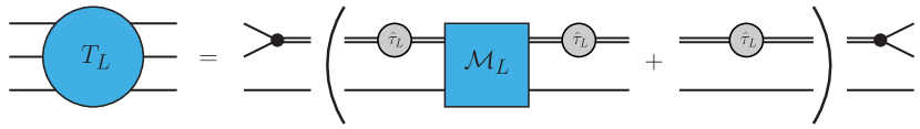
Figure 1: The three-particle scattering amplitude $T_{L}$, constructed from the particle-dimer scattering amplitude ${\cal M}_{L}$. The double line with a blob stands for the dressed dimer propagator. The quantity in the parentheses on the right hand side determines the finite volume spectrum and will be referred to as $\tilde{T}_{L}$ in the main text.

For definiteness, consider the scattering of a two-body bound state with binding energy $B_{2}>0$ and a third particle at a total center-of-mass energy $E$ in the infinite volume (we use the usual non-relativistic convention for $E$). There are the regions of three-body bound states ($E<-B_{2}$) and elastic scattering of the two-body bound state and the third particle ($-B_{2}\leq E<0$). Above the breakup threshold for the two-body bound state ($E=0$), three-body singularities from the free propagation of three-particle intermediate states appear in the interaction and the corresponding scattering amplitude SZ74 . Before the partial-wave projection, these singularities appear as single poles in the free three-body propagator. They are regulated by the usual $i\epsilon$ prescription that adds an infinitesimal positive imaginary part to the energy $E$. Integration over the solid angle, required for the partial-wave projection, transforms the poles to cuts with logarithmic branch points in the partial-wave amplitudes. The singularities of the partial-wave amplitudes are milder than before and the three-body poles in the original amplitude are restored only when the infinitely many partial waves are summed up. The branch points are in principle integrable in each partial wave but they lead to instabilities in numerical calculations if they are not handled with special care. In numerical solutions of the three-body scattering problem these cuts are thus usually treated via contour deformation (if the kernel is known analytically) or via the introduction of small but finite imaginary parts in the energy $E$ which are extrapolated to zero in the end. In practical calculations in the three-nucleon system, the partial-wave expansion then converges well, below and above breakup, see, e.g., Ref. Golak:2014ksa .

In the finite volume matters are different, as the whole spectrum is discrete. In a cubic box, only a discrete set of momenta determined by the boundary conditions (usually taken as periodic) is allowed. Therefore, the rotational symmetry is broken down to cubic symmetry including rotations and reflections, which form the octahedral group $O_{h}$. The infinitely many irreducible representations of the rotation group map onto the 10 irreducible representations of the octahedral group. Below the lowest inelastic threshold one can still expand in the infinite-volume partial waves, although they are coupled now due to the breaking of rotational symmetry Kreuzer:2008bi ; Kreuzer:2009jp ; Kreuzer:2010ti ; Polejaeva:2012ut ; Kreuzer:2012sr ; Hansen:2014eka ; pang2 . The partial-wave expansion for the interaction converges well in this region, since the regular summation theorem Luesch86 ; Doring:2012eu ensures that the infinite-volume partial-wave projection remains a good approximation for regular interactions. Above the inelastic thresholds, the finite-volume interaction has discrete poles from three-body intermediate states. This averts the convergence of the partial-wave expansion, making the expansion in eigenfunctions of the octahedral symmetry group unavoidable in this energy region. Definition and implementation of such an expansion for the three-body quantization condition is the aim of the current study. We shall in particular demonstrate that, owing to the octahedral symmetry, the three-body quantization condition pang1 ; pang2 ; Mai:2017bge ; Briceno:2017tce ; Hansen:2016fzj ; Hansen:2015zta ; Hansen:2015zga ; Hansen:2014eka ; Polejaeva:2012ut ; Briceno:2012rv ; Roca:2012rx can be split into different independent equations, whose solutions determine the finite-volume energy spectrum in different irreducible representations (irreps) of the octahedral group. This is extremely convenient, since the source/sink operators in lattice calculations are usually chosen to transform as irreducible tensor operators under the octahedral group, allowing one to determine the energy spectra in different irreps independently.

In this paper, we present two equivalent methods to implement the above expansion with different technical advantages. The plan of the paper is as follows. In Section II, we discuss the three-particle quantization condition and, in particular, various singularities, appearing there. In Sections III and IV, we describe both diagonalization procedures for the quantization condition in the basis functions of different irreps. Finally, Section V contains an example of a numerical solution of the quantization condition involving the projection method. The interpretation of the energy levels in terms of the bound and scattering states is also discussed. Technical details are relegated to the appendices.

II Three-particle quantization condition

The three-body quantization condition can be derived in the particle-dimer picture used in Refs. pang1 ; pang2 or the spectator-isobar picture used in Refs. Mai:2017bge . As far as the quantization condition is concerned, the formal differences play no role. Therefore, in the following we refer in many occasions to both as “dimers” for simplicity. To describe the interactions in the three-particle system within this picture, one needs the following blocks: the two-particle interactions, characterized by the dimers (isobars) and the interaction of the dimer (isobar) with the third particle (spectator). Two important remarks are in order. First, the dimer picture is not an approximation, but an equivalent description of the three-particle system, if one allows for dimers of any spin and for a generic two-particle-dimer vertex pang1 ; pang2 . This corresponds to the partial-wave expansion in the two-body amplitude. Second, the dimer formalism does not necessarily imply the presence of a shallow two-body bound-state (resonance), albeit in this case the use of this formalism might be more efficient, since one term will dominate the expansion of the two-body scattering amplitude. Both statements are self-evident in effective field theory, where the dimer field is just a dummy integration variable in the path integral Bedaque:1998kg ; Bedaque:1998km ; Bedaque:1999vb . However, their validity does not depend, of course, on a particular framework used. For example, in Ref. Mai:2017vot the two-body interaction in a given partial wave is parameterized by an amplitude obtained within the $N/D$ method, with the analytic properties directly determined from the three-body unitarity. Nevertheless, all final expressions are similar to those obtained in the effective field theory framework.

In a finite volume, the energy levels coincide with the position of the poles of the finite-volume three-particle amplitude. This amplitude can be related to the particle-dimer scattering amplitude – schematically, this relation is depicted in Fig. 1. Since the external vertices (outside the brackets in Fig. 1) are non-singular, they can be left out. The remaining piece of the finite-volume amplitude, which is depicted in the parentheses on the right hand side of Fig. 1, reads as

$$\tilde{T}_{L}({\bf p},{\bf q};E)=\hat{\tau}_{L}({\bf p};E)\,{\cal M}_{L}({\bf p},{\bf q};E)\, \hat{\tau}_{L}({\bf q};E)$$ (1)

$$+\hat{\tau}_{L}({\bf p};E)\,L^{3}\delta_{{\bf p}{\bf q}}\,,$$

where $L$ denotes the spatial size of the box, $E$ is the total energy of the three particles, and ${\bf p}$ and ${\bf q}$ are the discretized relative dimer-spectator three-momenta, e.g., ${\bf p}\in\{2\pi{\bf n}/L|{\bf n}\in\mathbb{Z}^{3}\}$. The particle-dimer scattering amplitude obeys the Bethe-Salpeter equation

$${\cal M}_{L}({\bf p},{\bf q};E )=Z({\bf p},{\bf q};E)$$ (2)

$$+\frac{1}{L^{3}}\,\sum_{\bf k}^{\Lambda}Z({\bf p},{\bf k};E)\,\hat{\tau}_{L}({\bf k};E)\,{\cal M}_{L}({\bf k},{\bf q};E)\,,$$

where $\Lambda$ is the ultraviolet cutoff and $\hat{\tau}_{L}$ stands for the dressed dimer propagator. Assuming, for instance, the non-relativistic kinematics as in Refs. pang1 ; pang2 , we have:

$$8\pi\hat{\tau}_{L}^{-1}({\bf k};E) = k^{*}\cot\delta(k^{*})+S({\bf k},(k^{*})^{2})\,,$$ (3)

$$S({\bf k},(k^{*})^{2}) = -\frac{4\pi}{L^{3}}\sum_{\bf l}\frac{1}{{\bf k}^{2}+{\bf k}{\bf l}+{\bf l}^{2}-mE}\,,$$

where $k^{*}$ is the magnitude of the relative momentum of the pair in the rest frame,

$$k^{*}=\sqrt{\frac{3}{4}\,{\bf k}^{2}-mE}\,.$$ (4)

In Eq. (3), unlike Eq. (2), the momentum sum is implicitly regularized by using dimensional regularization and $\delta(k^{*})$ is the S-wave phase shift in the two-particle subsystem. The effective range expansion reads

$$k^{*}\cot\delta(k^{*})=-\frac{1}{a}+\frac{1}{2}\,r(k^{*})^{2}+O((k^{*})^{4})\,,$$ (5)

where $a,r$ are the two-body scattering length and the effective range, respectively. For simplicity, we shall consider the case, when the two-body interactions are described only by the scattering length $a$. The effective range $r$ and higher-order shape parameters are all set equal to zero, corresponding to the leading order of the effective field theory for short range-interactions Bedaque:1998kg ; Bedaque:1998km .

Finally, the quantity $Z$ denotes the kernel of the Bethe-Salpeter equation. It contains the one-particle exchange diagram, as well as the local term, corresponding to the particle-dimer interaction (three-particle force). Again, for simplicity, we shall restrict ourselves to the case of non-derivative coupling, which is described by a single constant $H_{0}(\Lambda)$. The kernel then takes the form

$$Z({\bf p},{\bf q};E)=\frac{1}{-mE+{\bf p}^{2}+{\bf q}^{2}+{\bf p}{\bf q}}+\frac{H_{0}(\Lambda)}{\Lambda^{2}}\,.$$ (6)

The dependence of $H_{0}(\Lambda)$ on the cutoff is such that the infinite-volume scattering amplitude is cutoff-independent. In a finite volume, this ensures the cutoff-independence of the spectrum.

We would like to stress here that using the effective range approximation, or restricting ourselves to the non-derivative particle-dimer interactions does not affect the generality of the following arguments. The equations like Eq. (6) are displayed here for the illustrative purpose only. In Refs. Mai:2017vot ; Mai:2017bge , both the two-body scattering amplitude and the three-body force depend on the momenta in a non-trivial way and the expression of the kernel gets modified. The main reason is the relativistic formulation of Refs. Mai:2017vot ; Mai:2017bge plus the fact that the vertices in general have momentum dependence which would correspond to inclusion of higher orders in the effective field theory language. However, all statements made in the present section apply in this case as well, since the singularity structure of the kernel remains the same. Specifically, unitarity ensures that the exchange singularity is the only one leading to imaginary parts of the interaction. Furthermore, three-body unitarity determines the imaginary parts from which real parts can be obtained using dispersion relations without any regularization issues using sufficiently many subtractions. Of course, the amplitude can be mapped to field theory if desired but there is no need to do so. In that framework, the term $H_{0}$ in Eq. (6) plays the role of a term that does not violate unitarity and that can be used to accommodate genuine three-body forces. The dispersive framework of Ref. Mai:2017vot also shows that the isobar picture simply provides a convenient parameterization and can be dropped in favor of unitary on-shell $2\to 2$ amplitudes formulated in any parameterization, plus real-valued three-body forces.

In a finite volume, close to a finite-volume pole of $\mathcal{M}_{L}$ at $E_{i}$, the amplitude factorizes and can be written in the form

$$\mathcal{M}_{L}({\bf p},{\bf q};E)=\frac{f_{i}({\bf p})f^{*}_{i}({\bf q})}{E-E_{i}}\,.$$ (7)

Substituting this expression into the Eq. (2) and dropping the parametric dependence on the momentum ${\bf q}$, a homogeneous equation can be obtained

$$f_{i}({\bf p})=\frac{1}{L^{3}}\sum_{\bf k}^{\Lambda}Z({\bf p},{\bf k};E)\hat{\tau}_{L}({\bf k};E)f_{i}({\bf k}).$$ (8)

Here the inhomogeneous term has been dropped, because it can never develop a pole in the energy.

The quantization condition is obtained from the above equations in a trivial fashion. Symbolically, the solution for $\tilde{T}_{L}$ is given by:

$$\tilde{T}_{L}=(\hat{\tau}_{L}^{-1}-Z)^{-1}\,.$$ (9)

The quantity $\tilde{T}_{L}$ has poles, when the determinant of the inverse of the r.h.s. of Eq. (9) vanishes. This finally gives the quantization condition we are looking for,

$$\det(\hat{\tau}_{L}^{-1}-Z)=0\,.$$ (10)

The l.h.s. of the above equation defines a function of the total energy $E$, which, for a fixed $\Lambda$ and $L$, depends both on the two-body input (the two-body scattering amplitude both above and below the two-body threshold) as well as the three-body input (the non-derivative coupling $H_{0}(\Lambda)$ plus higher-order couplings). The former input can be independently determined from the simulations in the two-particle sector and extrapolation below threshold. Hence, measuring the three-particle energy levels, one will be able to fit the parameters of the three-body force. Finally, using the same equations in the infinite volume with the parameters determined on the lattice, one is able to predict the physical observables in the infinite volume.

An important remark is in order. The finite-volume spectrum of the three-particle system is uniquely determined by the poles of the three-particle amplitude $T_{L}$ (or $\tilde{T}_{L}$, because the insertions in the external lines are not singular, see Fig. 1). It means that every root of Eq. (10) corresponds to an energy level, and vice versa. On the other hand, as it has been noted independently in Refs. Mai:2017bge ; pang2 , both $\hat{\tau}_{L}^{-1}$ and $Z$ become singular at certain energies, which leads to the fact that the particle-dimer amplitude ${\cal M}_{L}$ will contain both, poles corresponding to the genuine three-body levels and spurious poles arising from these singularities. In the amplitude $\tilde{T}_{L}$ these poles are canceled automatically. This was noted and described in detail in Ref. Mai:2017bge , see also Refs. Polejaeva:2012ut ; Briceno:2012rv . This cancellation rests on two essential observations:

1. At the energies, where $Z$ becomes infinite, $\hat{\tau}_{L}$ is exactly zero. Physically, the reason is three-body unitarity, which restricts the singularity structure of these quantities Mai:2017bge .

2. The dressed propagator of the dimer is singular at real energies, corresponding to the two-particle energy levels in a finite volume. This singularity is canceled in $\tilde{T}_{L}$ if the disconnected piece (the second term on the r.h.s. of Fig. 1 or of Eq. (2)) is included Mai:2017bge . Physically, this is due to the LSZ-reduction formula, which relates the full $S$-matrix elements (including all possible clusterings of transitions) to the correlation functions of the underlying field theory which, by definition, do not have these singularities.

The cancellation considered above guarantees that there are no spurious poles in the quantization condition, see Eq. (10).

III Projection onto the irreps

As already mentioned, the quantization condition, Eq. (10), determines the entire spectrum of the three-body system. It would be useful to partially diagonalize this equation, projecting it to the various irreps of the octahedral group – in particular because, in practice, the energy levels corresponding to a given irrep are extracted on the lattice. Moreover, Eq. (10) may, in general, contain very large matrices. Namely, the matrices $\hat{\tau}_{L}$ and $Z$ have dimension $N^{3}\times N^{3}$, where $N$ is the largest integer that does not exceed $\Lambda L/(2\pi)$. The projection of the quantization condition to a given irrep allows one to reduce the dimension of the matrices.

In this section, we describe how such a projection, which qualitatively resembles the partial-wave expansion in the infinite volume, can be performed. As discussed in the introduction, this becomes necessary due to the occurrence of three-body singularities. For two-body systems this step is not required because the two-body interactions are regular and the regular summation theorem applies.

III.1 The group and its irreps

The symmetry group ${\cal G}$ of the cubic lattice in the rest frame is the octahedral group that consists of 24 rotations $R_{a}$ and the inversion $I$ of all axes. These rotations with $a=1,\ldots,24$ can be characterized either by the unit vector ${\bf n}^{(a)}$ along the rotation axis and angle $\omega_{a}$, or, equivalently, by three Euler angles $\alpha_{a},\beta_{a},\gamma_{a}$, given, e.g., in table A.1 of Ref. Bernard:2008ax . A general element of the group ${\cal G}$ is given by $g=R_{a}I$, where $I$ commutes with all $R_{a}$, i.e., the total number of the elements of ${\cal G}$ is equal to $48$. The irreps of the octahedral group of 24 elements (pure rotations) are

• the trivial one-dimensional representation which assigns $+1$ to all 24 elements of the group.

• the one-dimensional representation, which assigns $-1$ to the rotations from the conjugacy classes $6C_{4}$, $6C_{2}^{\prime}$ (see table A.1 of Ref. Bernard:2008ax ) and $+1$ otherwise.

• the two-dimensional representation. The corresponding matrices are given, e.g., in Eq. (A.2) of Ref. Bernard:2008ax .

• the three-dimensional representation. The corresponding matrices are given via the rotation parameters

  $$T_{\sigma\rho}(R_{a}) =\cos\omega_{a}\delta_{\sigma\rho}$$ (11)

  $$+(1-\cos\omega_{a})n^{(a)}_{\sigma}n^{(a)}_{\rho}-\sin\omega_{a}\varepsilon_{\sigma\rho\lambda}n^{(a)}_{\lambda}\,.$$

  Here, the indices $\sigma,\rho,\lambda=1,2,3$ and $a=1,\ldots,24$ (no inversions).

• is the same with a change of sign in the conjugacy classes $6C_{4}$, $6C_{2}^{\prime}$ .

For convenience, we collect all these matrices in Appendix A.

Adding inversions, each of these representation duplicates, e.g., $A_{1}\to A_{1}^{\pm}$, etc. In these representations, the elements corresponding to $R$ and $RI$ are the same for “$+$” and have the opposite sign for “$-$”.

III.2 Shells

Our aim is to carry out an analog of the partial-wave expansion in momentum space in case of cubic symmetry. For this reason, we define the shells, which are the analog of the surface $|{\bf p}|=\mbox{const.}$ in case of the rotational symmetry. In order to ease notations, we shall measure all momenta in units of $2\pi/L$ in this section.

• The (single) momentum with the smallest length is $(0,0,0)$. This defines the shell $s=1$. All 48 symmetry transformations, acting on this vector leave it invariant.

• The vectors with the second smallest length are $(1,0,0)$ and all vectors that are obtained from this vector by symmetry transformations, which always boil down to the permutation of components of a vector or a change of sign of one or several components. In this case, there are 6 different vectors which define the next shell, i.e. $s=2$ with the multiplicity $\vartheta(2)=6$. Furthermore, note once more that each vector in a shell is obtained through

  $${\bf p}=g\,{\bf p}_{0}\,,\quad\quad g\in{\cal G}\,.$$ (12)

  We shall refer to ${\bf p}_{0}$ to as reference vector of a given shell. Nothing depends on the choice of this vector.

• One can continue this procedure, consequently including the vectors with a larger length. At some point, one finds that there are vectors with the same length, which are nevertheless not related by the symmetry transformations. First, this situation arises for the sets with the reference vectors $(3,0,0)$ and $(2,2,1)$. We assign such vectors to different shells, $s=9$ and $s=10$ in this example. Thus, our definition of a shell implies that all vectors in a given shell are produced from one reference vector by applying symmetry transformations.

At this point, one may consider a spherically symmetric function, which depends only on the magnitude of ${\bf p}$. The rotation that transforms $(3,0,0)$ into $(2,2,1)$, albeit not belonging to ${\cal G}$, still leaves this function invariant – in other words, the symmetry of this function for a given $|{\bf p}|$ is larger than ${\cal G}$. It is clear that, going to higher shells, the number of the combinations of the vectors with the same length (in units of $2\pi/L$) is going to increase, rendering the symmetry larger. One may now fix $|{\bf p}|$ in physical units and increase $L$ – in a result, this vector will correspond to the shell(s) with a very high value of $s$ and hence with a very high degree of degeneracy. The above discussion provides a qualitative argument in favor of the conclusion that the rotation symmetry is restored in the limit $L\to\infty$.

III.3 Expansion in the irreps

An arbitrary function $f({\bf p})$ can be characterized by the shell to which the momentum ${\bf p}$ belongs, and the orientation of ${\bf p}$. Below, we aim at finding a counterpart of the well-known partial-wave expansion

$$f({\bf p}) =\sqrt{4\pi}\sum_{\ell m}Y_{\ell m}({\bf\hat{p}})f_{\ell m}(p)\,,$$ (13)

$$f_{\ell m}(p) =\frac{1}{\sqrt{4\pi}}\,\int d\Omega Y^{*}_{\ell m}({\bf\hat{p}})f({\bf p})$$

for the case of the cubic symmetry on the lattice. In the above expression, $Y_{\ell m}$ are spherical harmonics, and $p$, ${\bf\hat{p}}$ denote the magnitude and the unit vector in the direction of the vector ${\bf p}$, respectively.

On the cubic lattice, the analog of the above expansion is given by

$$f({\bf p})=f(g{\bf p}_{0})=\sum_{\Gamma}\sum_{\rho\sigma}T^{\Gamma}_{\sigma\rho}(g)f^{\Gamma}_{\rho\sigma}({\bf p}_{0})\,,$$ (14)

where $\Gamma=A_{1}^{\pm},A_{2}^{\pm},E^{\pm},T_{1}^{\pm},T_{2}^{\pm}$, and the matrices of the irreducible representations $T^{\Gamma}_{\sigma\rho}(g)$ are specified in Appendix A. Note also that $f^{\Gamma}_{\rho\sigma}({\bf p}_{0})=f^{\Gamma}_{\rho\sigma}(g{\bf p}_{0})$ for all $g\in{\cal G}$.

Using the orthogonality of the matrices of the irreducible representations, it is possible to project out the quantity $f^{\Gamma}_{\rho\sigma}({\bf p}_{0})$:

$$\sum_{g\in{\cal G}}(T^{\Gamma}_{\lambda\delta}(g))^{*}f(g{\bf p}_{0}) =\sum_{g\in{\cal G}}(T^{\Gamma}_{\lambda\delta}(g))^{*}\sum_{\Gamma^{\prime}}\sum_{\rho\sigma}T^{\Gamma^{\prime}}_{\sigma\rho}(g)f^{\Gamma^{\prime}}_{\rho\sigma}({\bf p}_{0})$$

$$=\sum_{\Gamma^{\prime}}\sum_{\rho\sigma}\frac{G}{s_{\Gamma}}\,\delta_{\Gamma\Gamma^{\prime}}\delta_{\sigma\lambda}\delta_{\rho\delta}f^{\Gamma^{\prime}}_{\rho\sigma}({\bf p}_{0})$$

$$=\frac{G}{s_{\Gamma}}\,f^{\Gamma}_{\delta\lambda}({\bf p}_{0})\,,$$ (15)

where $G=48$ is the total number of elements in the group ${\cal G}$ and $s_{\Gamma}$ is the dimension of the representation $\Gamma$: $s_{\Gamma}=1$ for $\Gamma=A_{1}^{\pm},A_{2}^{\pm}$, $s_{\Gamma}=2$ for $\Gamma=E^{\pm}$, $s_{\Gamma}=3$ for $\Gamma=T_{1}^{\pm},T_{2}^{\pm}$.

In order to clarify the meaning of the above expressions, let us assume that $f({\bf p})$ is a regular function which can be expanded in partial waves, see Eq. (13). Substituting this expansion into Eq. (III.3), one obtains

$$\frac{G}{s_{\Gamma}}f^{\Gamma}_{\rho\sigma}({\bf p}_{0})=\sqrt{4\pi}\sum_{\ell m}\sum_{g\in{\cal G}}(T^{\Gamma}_{\sigma\rho}(g))^{*}Y_{\ell m}(g{\bf\hat{p}}_{0})f_{\ell m}(p)\,.$$ (16)

Here, we used the fact that $|g{\bf p}_{0}|=|{\bf p}_{0}|=p$. Furthermore, we use the relation

$$Y_{\ell m}(g{\bf\hat{p}}_{0})=\sum_{m^{\prime}}\hat{D}^{(\ell)}_{mm^{\prime}}(g)Y_{\ell m^{\prime}}({\bf\hat{p}}_{0})\,,$$ (17)

where the quantity $\hat{D}^{(\ell)}_{mm^{\prime}}(g)$ is defined as follows: if $g$ is a pure rotation, then $\hat{D}^{(\ell)}_{mm^{\prime}}(g)$ coincides with the conventional Wigner matrix $D^{(\ell)}_{mm^{\prime}}(g)$; if $g$ contains the inversion, it can be represented as $g=R_{a}I$. Then, $\hat{D}^{(\ell)}_{mm^{\prime}}(g)=(-1)^{\ell}D^{(\ell)}_{mm^{\prime}}(R_{a})$.

It can be seen now that the vectors

$$\xi_{\rho\sigma m}^{\ell\Gamma}({\bf\hat{p}}_{0})=\sum_{g\in{\cal G}}(T^{\Gamma}_{\sigma\rho}(g))^{*}\sum_{m^{\prime}}\hat{D}^{(\ell)}_{mm^{\prime}}(g)Y_{\ell m^{\prime}}({\bf\hat{p}}_{0})$$ (18)

coincide with the basis vectors of the irrep $\Gamma$, corresponding to a given angular momentum $\ell$, see e.g., Refs. Bernard:2008ax ; Gockeler:2012yj . Namely, the indices $\sigma,\rho$ label the basis vectors, and $m$ the components of each vector. Consequently, the quantity $f^{\Gamma}_{\rho\sigma}({\bf p}_{0})$ can be expanded in the basis vectors of a particular irrep $\Gamma$:

$$f^{\Gamma}_{\rho\sigma}({\bf p}_{0})=\frac{{\sqrt{4\pi}}s_{\Gamma}}{G}\,\sum_{\ell m}f_{\ell m}(p)\xi_{\rho\sigma m}^{\ell\Gamma}({\bf\hat{p}}_{0})\,.$$ (19)

In Section IV, we will describe an alternative method to construct a minimal basis for a given shell $s$.

III.4 The projection of the quantization condition

The quantization condition can be obtained starting from (8). Hiding the dependence on the energy $E$ and level index $i$, we obtain

$$f({\bf p})=\frac{1}{L^{3}}\,\sum_{\bf k}Z({\bf p},{\bf k})\hat{\tau}_{L}({\bf k})f({\bf k})\,.$$ (20)

Moreover, the quantities $Z$ and $\hat{\tau}_{L}$ are scalars with respect to the group ${\cal G}$. This means that for all $g\in{\cal G}$

$$Z(g{\bf p},g{\bf k})=Z({\bf p},{\bf k})\,\quad\text{and}\quad\hat{\tau}_{L}(g{\bf k})=\hat{\tau}_{L}({\bf k})\,.$$ (21)

The summation over the lattice momenta ${\bf k}$ can be replaced by the summation over the shells $s$ and over the orientations of the momentum ${\bf k}$ inside a given shell $s$, which are described by ${\bf k}(s)=g{\bf k}_{0}(s),~{}g\in{\cal G}$ (here, we explicitly indicate the shell index $s$). Altogether, we have $\vartheta(s)$ different vectors, but $G$ terms in the sum over all elements of the group ${\cal G}$, so each vector will appear $G/\vartheta(s)$ times in this sum. Taking this fact into account, we may rewrite Eq. (20) in the following form

$$f({\bf p})=\frac{1}{L^{3}}\,\sum_{s}\sum_{g\in{\cal G}}\frac{\vartheta(s)\hat{\tau}_{L}(s)}{G}\,Z({\bf p},g{\bf k}_{0}(s))f({\bf k})\,.$$ (22)

Here, we used the fact that $\hat{\tau}_{L}({\bf k})$ does not depend on the orientation of ${\bf k}$ in a given shell, i.e., that it is a function of the shell index only.

Multiplying now this equation with $(T^{\Gamma}_{\sigma\lambda}(g^{\prime}))^{*}$ from the left and using Eqs. (14, III.3), we obtain

$$\frac{G}{s_{\Gamma}}\,f^{\Gamma}_{\lambda\sigma}(r)=\frac{1}{L^{3}}\,\sum_{s}\frac{\vartheta(s)\hat{\tau}_{L}(s)}{G}\,\sum_{\Gamma^{\prime}}\sum_{\rho\delta}Z^{(\Gamma\Gamma^{\prime})}_{\lambda\sigma,\rho\delta}(r,s)f^{\Gamma^{\prime}}_{\rho\delta}(s)\,,$$ (23)

where we have adjusted a notation $f^{\Gamma}_{\lambda\sigma}({\bf p}_{0}(r))\to f^{\Gamma}_{\lambda\sigma}(r)$. Furthermore, in the above equation,

$$Z^{(\Gamma\Gamma^{\prime})}_{\lambda\sigma,\rho\delta}(r,s)=\sum_{g,g^{\prime}\in{\cal G}}(T^{\Gamma}_{\sigma\lambda}(g^{\prime}))^{*}Z(g^{\prime}{\bf p}_{0}(r),g{\bf k}_{0}(s))T^{\Gamma^{\prime}}_{\delta\rho}(g)$$

$$=\sum_{g,g^{\prime}\in{\cal G}}(T^{\Gamma}_{\sigma\lambda}(g^{\prime}))^{*}Z(\underbrace{g^{-1}g^{\prime}}_{=g^{\prime\prime}}{\bf p}_{0}(r),{\bf k}_{0}(s))T^{\Gamma^{\prime}}_{\delta\rho}(g)$$

$$=\sum_{g,g^{\prime\prime}\in{\cal G}}(T^{\Gamma}_{\sigma\lambda}(gg^{\prime\prime}))^{*}Z(g^{\prime\prime}{\bf p}_{0}(r),{\bf k}_{0}(s))T^{\Gamma^{\prime}}_{\delta\rho}(g)$$

$$=\sum_{g,g^{\prime\prime}\in{\cal G}}\sum_{\omega}(T^{\Gamma}_{\sigma\omega}(g))^{*}(T^{\Gamma}_{\omega\lambda}(g^{\prime\prime}))^{*}Z(g^{\prime\prime}{\bf p}_{0}(r),{\bf k}_{0}(s))T^{\Gamma^{\prime}}_{\delta\rho}(g)$$

$$=\sum_{g^{\prime\prime}\in{\cal G}}\sum_{\omega}\frac{G}{s_{\Gamma}}\,\delta_{\Gamma\Gamma^{\prime}}\delta_{\sigma\delta}\delta_{\omega\rho}(T^{\Gamma}_{\omega\lambda}(g^{\prime\prime}))^{*}Z(g^{\prime\prime}{\bf p}_{0}(r),{\bf k}_{0}(s))$$

$$=\frac{G}{s_{\Gamma}}\,\delta_{\Gamma\Gamma^{\prime}}\delta_{\sigma\delta}\sum_{g\in{\cal G}}(T^{\Gamma}_{\rho\lambda}(g))^{*}Z(g{\bf p}_{0}(r),{\bf k}_{0}(s))$$

$$\doteq\frac{G}{s_{\Gamma}}\,\delta_{\Gamma\Gamma^{\prime}}\delta_{\sigma\delta}Z^{\Gamma}_{\lambda\rho}(r,s)\,.$$ (24)

Using this result, we can rewrite Eq. (23) as

$$f^{\Gamma}_{\lambda\sigma}(r)=\frac{1}{L^{3}}\,\sum_{s}\frac{\vartheta(s)\hat{\tau}_{L}(s)}{G}\,\sum_{\rho}Z^{\Gamma}_{\lambda\rho}(r,s)f^{\Gamma}_{\rho\sigma}(s)\,.$$ (25)

Note that, due to the symmetry, $Z^{\Gamma}_{\lambda\rho}(r,s)$ and hence $f^{\Gamma}_{\rho\sigma}(s)$ do not depend on $\sigma$.

Finally, the quantization condition in a given irrep $\Gamma$ takes the form

$$\det\biggl{(}\hat{\tau}_{L}(s)^{-1}\delta_{rs}\delta_{\sigma\rho}-\frac{\vartheta(s)}{GL^{3}}\,Z^{\Gamma}_{\sigma\rho}(r,s)\biggr{)}=0\,.$$ (26)

Note that, on a given shell, the quantity $Z^{\Gamma}_{\sigma\rho}(r,s)$ may vanish for certain $\Gamma$. A trivial example: as seen from Eq. (III.4), all sums except $\Gamma=A_{1}^{+}$ vanish on the first shell $r=1$ or $s=1$. In the calculation of the determinant, one could first “compress” the matrix $Z^{\Gamma}_{\sigma\rho}(r,s)$ by deleting all rows/columns which consist only of zeros. The three-particle quantization condition, projected onto the different irreps, which is displayed in Eq. (26), represents our main result. The shells are truncated by using a sharp cutoff at $N=\Lambda L/(2\pi)$. We emphasize that the solution of the quantization condition, Eq. (26), is cutoff-independent. This happens because the cutoff-dependence of the effective couplings $H_{0}(\Lambda),H_{2}(\Lambda),\cdots$ ensures that the physical observables in the infinite volume are cutoff-independent. At the same time, the finite-volume spectrum becomes cutoff-independent as well, since at short distances (of order of $1/\Lambda$), the effect of a finite-size box is not felt.

In a concluding remark we address the issue of partial-wave mixing in Eq. (26). There are two angular momenta in the problem: the angular momentum $\ell$ of the spectator-dimer system and the internal angular momentum $\ell^{\prime}$ of the dimer (the dimer spin). The dimer spin $\ell^{\prime}$ corresponds to the angular momentum of the interacting particle pair and is kept as zero throughout this paper, while $\ell$ can be arbitrary. Obviously, the $\ell^{\prime}=0$ particle-particle interactions generate contributions corresponding to all values of $\ell$ in the projected interaction kernel $Z^{\Gamma}$ in Eq. (26). Therefore, if one truncates the expansion of the polynomial term at $\ell=0$ as in Eq. (6), the energy levels in Eq. (26) are determined by the S-wave couplings only.

The inclusion of the higher partial waves proceeds in the standard fashion described, e.g., in Refs. pang1 ; pang2 . On the opposite, if one expands in the conventional spherical functions instead of the basis functions of the irreps of the octahedral group, as was done, e.g., in Refs. Kreuzer:2008bi ; Kreuzer:2009jp ; Kreuzer:2010ti ; Kreuzer:2012sr ; pang2 , one gets the partial-wave mixing already in the presence of the S-wave couplings only. It is clear that this mixing is hand-made and can be avoided, if the method described in this section is used.

IV Expansion in cubic harmonics

In the following, we describe an alternative method for the projection of the scattering amplitudes to different irreps which resembles the usual projection to partial waves in the infinite volume. Such a procedure was already applied in Ref. Mai:2017bge for the irrep $A_{1}^{+}$, but is generalized here. Finally, we will make a comparison of this method with the one presented in the previous section.

The momentum shells in the new approach are defined as in Section III.2. Furthermore, we define the finite-volume scalar product for any two functions $f$ and $g$ on a given shell $s$ by

$$\langle f,g\rangle_{s}=\frac{4\pi}{\vartheta(s)}\,\sum_{j}^{\vartheta(s)}f({\bf\hat{p}}_{j})^{*}g({\bf\hat{p}}_{j})\,,$$ (27)

where the sum runs over the $\vartheta(s)$ different orientations of the unit vector ${\bf\hat{p}}_{j}$ pointing to point $j$ in a given shell.

Our aim is to construct an orthonormal basis with respect to this scalar product, which allows one to expand an arbitrary function $f({{\bf\hat{p}}})$ into a linear combination of the basis vectors on a given shell. Each vector is a function of the ${\bf\hat{p}}_{j}$ (we therefore refer also to “basis functions”). In fact, this is an analog of the standard partial-wave expansion, Eq. (13), with some significant differences. First of all, in contrast to the basis functions on the unit sphere in infinite volume (such as spherical harmonics $Y_{\ell m}({\bf\hat{p}})$), the full set of basis functions in finite volume is given by a finite set of the so-called cubic harmonics $X_{\ell}^{\Gamma\nu\alpha}({\bf\hat{p}})$ where $\Gamma$ denotes, as before, the irrep of the octahedral group and $\alpha$ specifies the basis vector in the given irrep. The additional indices $\ell$ and $\nu$ specify the angular momentum (see Eq. (28)) and the degeneracy at that $\ell$, respectively.

The cubic harmonics are linear combinations of spherical harmonics, see, e.g., Refs. Bernard:2008ax ; Gockeler:2012yj and can be obtained by using the projection operators defined in Eq. (18) – more precisely, they can be identified with different components (labeled by the index $m$) of the vector $\xi$ in Eq. (18). The final result reads

$$X_{\ell}^{\Gamma\nu\alpha}({\bf\hat{p}})=\sum_{m}c_{\ell m}^{\Gamma\nu\alpha}Y_{\ell m}({\bf\hat{p}})\,.$$ (28)

These functions are orthogonal in $\Gamma$ and $\alpha$ with respect to the infinite-volume scalar product, and the $c_{\ell m}^{\Gamma\nu\alpha}$ are Clebsch-Gordan coefficients.

Evidently, on any shell the number of points cannot be larger than the number of elements in the cubic group $G=48$, and it changes from shell to shell according to Sec. III.2. A useful observation in this respect is that all shells can be characterized by the following seven types

$$(000),~{}(00b),~{}(0bb),~{}(bbb),~{}(0bc),~{}(bbc),~{}(bcd)\ ,$$ (29)

where all non-negative integers $0$, $b$, $c$, and $d$ are different, $x\neq y$ for $x,\,y\in\{0,b,c,d\}$. Each type specifies one point of the shell which through the symmetry transformations of the cubic group gives rise to all points in the shell. The multiplicity $\vartheta$ is unique for all shells of a given type as specified in Tab. 2.

Let us now start constructing the basis functions for each individual shell. Clearly, any function defined on the shell of type $(000)$ does not depend on momenta at all and is proportional to the cubic harmonic $X_{0}^{A_{1}^{+}11}$ which, therefore, is the sole basis vector on this shell. Other types of shells contain more points (are of higher multiplicity $\vartheta$), which coincides with the size of the maximal linear independent set of cubic harmonics. It is possible to make a unitary transformation such that all cubic harmonics are manifestly real. Conveniently one can use the following iterative procedure to determine such a set. We begin with the set $S:=\{X_{0}^{A_{1}^{+}11}\}$ and define the matrix

$$r_{mn}^{s}=\langle X_{m},X_{n}\rangle_{s}~{}~{}\text{for}~{}~{}X_{m},X_{n}\in S\,,$$ (30)

where the matrix $r$ depends explicitly on the shell index $s$. The indices $m$ and $n$ are cumulative, i.e., they comprise $\Gamma$, $\nu$, $\alpha$, and $\ell$. The set $S$ contains only one element, therefore the rank of the above $1\times 1$ matrix is $1$. If the multiplicity of the shell is also $1$ (for type $(000)$), then the set is complete and one stops here. If not, we add successively other cubic harmonics with increasing $\ell$ and different $\Gamma$, $\alpha$ and $\nu$ to set $S$, each time only keeping those, which increase the rank of the matrix $r$, and omitting the rest. When the rank of the matrix $r$ reaches the multiplicity of the given shell, the set $S$ contains the maximal number of linearly independent vectors and the procedure terminates – adding new harmonics cannot increase the rank anymore. For the afore-defined procedure, the cubic harmonics of $\ell\leq 9$ are required to build maximal sets on each of the seven types of shells. This is seen in Tab. 2, which is given in Appendix B.

It is important to note also that, according to the Wigner-Eckart theorem, the matrix $r^{s}$ is diagonal in the indices $\Gamma$ and $\alpha$, taking the block-diagonal form:

$$r^{s}_{mn}=\delta_{\Gamma\Gamma^{\prime}}\delta_{\alpha\alpha^{\prime}}r^{\Gamma s}_{uu^{\prime}}\,,$$ (31)

where the matrix $r^{\Gamma s}_{uu^{\prime}}$ does not depend on $\alpha$, and $u{}^{(}{{}^{\prime}}{}^{)}$ denotes a generalized index collecting combinations of $\nu{}^{(}{{}^{\prime}}{}^{)}$ and $l{}^{(}{{}^{\prime}}{}^{)}$. Thus, the above-described procedure can be carried out for the each irrep $\Gamma$ separately – the different irreps do not talk to each other.

Finally, the orthonormal basis

$$U_{s}:=\{\chi_{m}({\bf\hat{p}})|m=1,..,\vartheta(s)\}$$ (32)

on a given shell $s$ can be constructed by orthonormalizing the linearly independent $X_{m}$ with the use of the matrix $\zeta^{s}:=(r^{s})^{-1/2}$ as

$$\chi_{m}({\bf\hat{p}})\doteq\chi^{\Gamma\alpha s}_{u}({\bf\hat{p}})=\sum_{n}(\zeta_{mn}^{s})^{*}\hat{X}_{n}({\bf\hat{p}})\,,$$ (33)

where $m,n=1,..,\vartheta(s)$, while $u$ labels now the basis vectors for a given $\Gamma$ and $\alpha$ on shell $s$ and

$$\langle\chi_{m},\chi_{n}\rangle_{s}=\sum_{m^{\prime},n^{\prime}}\zeta^{s}_{mm^{\prime}}\,r^{s}_{m^{\prime}n^{\prime}}\,(\zeta^{s})^{*}_{nn^{\prime}}=\delta_{mn}\,.$$ (34)

Finally, we note that, while the orthonormalization procedure depends explicitly on the shell index $s$, the maximal set of linear independent cubic harmonics, see Tab. 2, depends only on the type of the shell. As an example, Tab. 2 in Appendix B shows that, for the shell type $(bcd)$, $\Gamma=T_{1}^{+}$, and $\alpha=1$, there are three cubic harmonics participating; their linear superpositions lead to the three basis vectors $\chi_{u}^{T_{1}^{+}1s}$ with $u=1,\dots,3$. In general, examining this table, one may conclude that the maximum number of the linearly independent basis vectors $\chi_{u}^{\Gamma\alpha s}$ for a given $\Gamma$ and $\alpha$ for all types of shells is given by the dimension $s_{\Gamma}$ of the irrep $\Gamma$. The basis vectors for the first 200 shells are numerically provided in the supplemental material of this manuscript.

With the orthonormal basis $U_{s}$ on a given shell $s$, any function defined on the points of this shell can be expanded similarly to the partial-wave projection Eq. (13) in infinite volume. We indicate the function defined at momentum ${\bf p}_{j}=|{\bf p}|{\bf\hat{p}}_{j}$ as $f^{s}({\bf\hat{p}}_{j})$ where ${\bf p}$ is the momentum associated with shell $s$. The expansion in basis functions reads now

$$f^{s}({\bf\hat{p}}_{j}) =\sqrt{4\pi}\sum_{\Gamma\alpha}\sum_{u}f^{\Gamma\alpha s}_{u}\chi_{u}^{\Gamma\alpha s}({\bf\hat{p}}_{j})\,,$$ (35)

$$f^{\Gamma\alpha s}_{u} =\frac{\sqrt{4\pi}}{\vartheta(s)}\,\sum_{j=1}^{\vartheta(s)}f^{s}({\bf\hat{p}}_{j})\chi^{\Gamma\alpha s}_{u}({\bf\hat{p}}_{j})\,~{}~{}\text{for}~{}~{}\chi^{\Gamma\alpha s}_{u}({\bf\hat{p}})\in U_{s}\,,$$

where $U_{s}$ is defined in Eq. (32) and the sum over $u$ is restricted to the number of basis vectors for a given $\Gamma$, $\alpha$, $s$.

The dimer-spectator amplitude (see Eq. (1) as well as Ref. Mai:2017bge ) depends on both incoming and outgoing momenta ${\bf p}$ and ${\bf p}^{\prime}$, therefore a decomposition into irreps for both momenta is required. We consider here this obvious generalization, assuming rotational symmetry for the transition $Z^{ss^{\prime}}({\bf\hat{p}}_{j},{\bf\hat{p}}_{j^{\prime}})$ as done throughout this paper. Here, ${\bf\hat{p}}_{j}$ (${\bf\hat{p}}_{j^{\prime}}$) is the direction of point $j$ ($j^{\prime}$) on shell $s$ ($s^{\prime}$). Due to rotational invariance and Schur’s lemma, the projections to the two- and three-dimensional irreps do not depend on the respective basis vectors $\alpha$. The result can then be written as

$$Z^{ss^{\prime}}({\bf\hat{p}}_{j},{\bf\hat{p}}_{j^{\prime}})=4\pi\sum_{\Gamma\alpha}\sum_{uu^{\prime}}\chi_{u}^{\Gamma\alpha s}({\bf\hat{p}}_{j})Z^{\Gamma ss^{\prime}}_{uu^{\prime}}\chi_{u^{\prime}}^{\Gamma\alpha s^{\prime}}({\bf\hat{p}}_{j^{\prime}})\,,$$ (36)

$$Z^{\Gamma ss^{\prime}}_{uu^{\prime}}=\frac{4\pi}{\vartheta(s)\vartheta(s^{\prime})}\,\sum_{j=1}^{\vartheta(s)}\sum_{j^{\prime}=1}^{\vartheta(s^{\prime})}\chi^{\Gamma\alpha s}_{u}({\bf\hat{p}}_{j})Z^{ss^{\prime}}({\bf\hat{p}}_{j},{\bf\hat{p}}_{j^{\prime}})\chi^{\Gamma\alpha s^{\prime}}_{u^{\prime}}({\bf\hat{p}}_{j^{\prime}})\,$$

for $\chi^{\Gamma\alpha s}_{u}({\bf\hat{p}})\in U_{s}$. Moreover, the dependence on the total scattering energy is not explicitly displayed and $\alpha$ is arbitrary. Note that $Z^{\Gamma ss^{\prime}}_{uu^{\prime}}$ still depends on the indices $u$ and $u^{\prime}$, corresponding to the incoming and outgoing momenta. In general, one has a (trivial) coupled-channel problem in these indices, similar to Eq. (26). As we have seen, the maximum number of the coupled equations on a given shell and in a given irrep $\Gamma$ is given by $s_{\Gamma}$, like in Eq. (26). As mentioned before, the supplemental material to this manuscript provides all needed input (basis vectors, direction of points, correspondence between $s$ and $|{\bf p}|$) to make the numerical implementation of Eq. (36) very convenient.

For completeness, we also quote the general projection of the quantization condition for the three-body method of Ref. Mai:2017bge (there, only the projection to $A_{1}^{+}$ was considered). With Eq. (36) and Eq. (17) of Ref. Mai:2017bge one obtains the projection of the quantization condition onto the different irreps, adapted to the current notation,

$$\det\left(B^{\Gamma ss^{\prime}}_{uu^{\prime}}(W^{2})+\frac{2E_{s}\,L^{3}}{\vartheta(s)}\tau_{s}(W^{2})^{-1}\delta_{ss^{\prime}}\delta_{uu^{\prime}}\right)=0\,,$$ (37)

where the relativistic energy is given by $E_{s}=\sqrt{m^{2}+{\bf p}^{2}}$, with $|{\bf p}|$ being the momentum associated with shell $s$, and $W$ is the total energy of the three-particle system. The dimer-spectator interaction kernel $B^{ss^{\prime}}({\bf\hat{p}}_{j},{\bf\hat{p}}_{j^{\prime}};W^{2})$ and dimer propagator $\tau_{s}(W^{2})$ are given by Eq. (3) and Eq. (12) of Ref. Mai:2017bge , respectively. The rows (columns) of the matrices in Eq. (37) are labeled by the indices $s$ and $u$ ($s^{\prime}$ and $u^{\prime}$).

The quantization conditions Eq. (26) derived in Sec. III and Eq. (37) above are equivalent modulo the use of relativistic kinematics and higher-order terms in the kernel, see the discussion after Eq. (6). Comparing the two approaches, we note that the decomposition defined by Eq. (14) is the same for all shells. The price to pay for the generality of the method presented in Sec. III is that the proposed basis may be too large for a given shell. This does not preclude one from carrying out the reduction of the quantization condition, but may lead to the situation that many entries in the matrix $Z^{\Gamma}_{ij}(r,s)$ are equal to zero (see the discussion at the end of Sec. III.4). The approach of the present section relies on the maximal linearly independent set of cubic harmonics, which are determined universally for all shells, ordered by the 7 types described before (see Table 2). However, the orthonormalization of such a set (determination of the basis $U_{s}$) has to be carried out on each set separately. In summary, on a given shell, the basis vectors, selected from the abundant set of all vectors in the first approach (III.4), are related to the basis vectors $U_{s}$ by a unitary transformation.

V Numerical calculations

V.1 Description of the model

In the previous sections, we have projected the three-body quantization condition onto the different irreps of the octahedral group, see Eq. (26). In this section, we wish to demonstrate, how this equation can be solved, and to discuss the properties of the finite-volume spectrum both below and above the breakup threshold. To this end, we perform the calculations in the toy model, already used for the same purpose in Refs. Kreuzer:2008bi ; Kreuzer:2009jp ; Kreuzer:2010ti ; Kreuzer:2012sr ; pang2 . This model corresponds to the leading order of the effective field theory for short range-interactions Bedaque:1998kg ; Bedaque:1998km . Moreover, it gives us an opportunity to compare our results with previous calculations.

The toy model, used here, has two coupling constants. First, the two-body scattering phase shift is given solely in terms of the scattering length $a$ through $k\cot\delta(k)=-1/a$. Second, the particle-dimer interaction contains no derivatives and is described by a single coupling constant $H_{0}(\Lambda)$ ($\Lambda$ stands for the ultraviolet cutoff). The dimer propagator $\hat{\tau}_{L}$ and the kernel $Z$ in this model are given by Eqs. (3) and (6), respectively. What remains is to fix the values of all free parameters and carry out the calculation of the energy spectrum.

As in Refs. Kreuzer:2008bi ; Kreuzer:2009jp ; Kreuzer:2010ti ; Kreuzer:2012sr ; pang2 , we assume $m=1$ and $a=1$. All length scales are given in units of $a$. We further fix the cutoff $\Lambda=225$, assuming that it is high enough for all effects of order of $1/\Lambda$ to be neglected. One may now fix the dimensionless coupling $H_{0}(\Lambda)$ e.g., by demanding that the three-body bound state has a given binding energy $B_{3}$. Assuming $B_{3}=10$ gives $H_{0}(\Lambda)=0.192$.

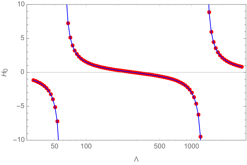
Figure 2: Running of $H_{0}(\Lambda)$ for $B_{3}=10$. Note that we take units with $m=a=1$.

What would happen, if one would choose another cutoff? Then, in order to obtain the same value of $B_{3}$, one would have to readjust $H_{0}(\Lambda)$. The outcome is shown in Fig. 2. It is clearly seen that the $\Lambda$-dependence of $H_{0}(\Lambda)$ exhibits the characteristic log-periodic behavior Bedaque:1998km ; Bedaque:1998kg . The essential point here is that fixing of one coupling constant guarantees the cutoff-independence of the whole tower of the Efimov states Efimov , as well as the particle-dimer scattering amplitude above threshold (up to the corrections of order of $1/\Lambda$). In the context of the problem we are considering, the study of the $\Lambda$-dependence is intertwined with the study of the large-$L$ behavior – recall that the dimension of the matrix in the quantization condition given in Eq. (10) is $N^{3}\times N^{3}$, where $N\simeq L\Lambda/(2\pi)$. Consequently, in order to study the scattering states in the limit $L\to\infty$ while keeping $N$ finite, one has to consider the small values of $\Lambda$ as well. Note here that the cutoff effects will not necessarily become large, since the energy of scattering states also tends to zero in this limit.

Let us now turn to the spectrum of the model – first, in the infinite volume:

1. In the two-body subsystem, there exists a bound dimer. The binding energy is

   $$B_{2}=\frac{1}{ma^{2}}=1\,.$$ (38)

   The typical momentum of a dimer is $1/a=1$ and its typical size is $a=1$.

2. We have adjusted the parameters such that there exists a three-particle bound state with the binding energy $B_{3}=10$. The corresponding bound-state momentum is $\kappa=\sqrt{mB_{3}}\simeq 3.162$ and the typical size is the inverse of this value. Since the characteristic size of the three-particle bound state is significantly smaller than that of the dimer, this state, to a certain approximation, can be considered as a bound state of three-particles (without clustering into a particle and a dimer).

3. One finds another bound state at $B_{3}=1.016$, corresponding to the bound-state momentum $\kappa=1.008$. We have now $\kappa^{2}-a^{-2}\ll\kappa^{2}$. Therefore, this state, to a good approximation, can be considered as a loosely bound state of a particle and a tightly bound dimer (see, e.g., Ref. pang1 ).

   Note also that the ratio of two energies $10/1.016\simeq 10$ strongly deviates from the value $515.03$, which is predicted by universality in the limit of infinitely large scattering length, $a\to\infty$. The typical size of the state with smaller binding energy, however, is much larger than the scattering length $a$.

Thus, in the infinite volume, we have a bound dimer and two three-body bound states. In a finite volume, we expect:

1. Two bound states, with the energies which are equal to those in the continuum up to exponentially suppressed corrections.

2. A tower of the particle-dimer scattering states in the CM frame, with the particle and dimer having quantized back-to-back momenta. In the limit $L\to\infty$, all these states tend to the threshold $E=-1$ (the sum of the particle and dimer masses minus $3m$).

3. A tower of three-particle scattering states with zero total momentum. In the limit $L\to\infty$, all these states should approach the threshold $E=0$.

In the actual calculations all energies will be slightly displaced from the free values, due to the interactions among the particles.

V.2 The entire energy spectrum

In the following, we will examine whether our expectation is indeed realized in the toy model defined in Eqs. (3,5,6). To do so, we project the quantization condition (37) to the irrep $A_{1}^{+}$, see Eq. (26). The projection of the kernel onto this irrep, see Eq. (III.4), gives

$$Z^{A_{1}^{+}}(r,s)= \sum_{g\in{\cal G}}Z(g\mathbf{p}_{0}(r),\mathbf{k}_{0}(s)),$$ (39)

which will be used in the three-body quantization condition, Eq. (26). The indices $\sigma,\rho$ are dropped since the irrep $A_{1}^{+}$ is one-dimensional.

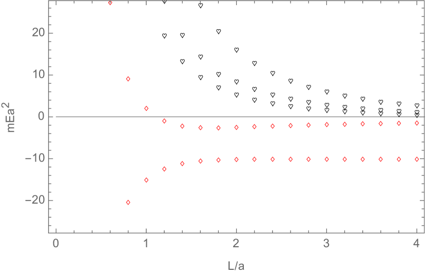
Figure 3: $L$-dependence of the energy levels of the toy model projected to $A_{1}^{+}$ irrep, determined from the solutions of Eq. (26) both below and above the threshold. Red diamonds and black hearts denote bound states and scattering states, respectively.

The entire spectrum (lowest-lying levels), obtained from the solution of the quantization condition is shown in Fig. 3 for different values of $L$.

V.3 Bound states

The two lowest levels in Fig. 3 tend to $E=-10$ and $E=-1.016$, respectively. As discussed above, the lowest energy level must look more like a bound state of three particles, so one expects that its $L$-dependence is described by the formula derived in Ref. Meissner:2014dea , see also Refs. Hansen:2016ync ; pang1 :

$$E_{L}-E_{\infty}=\frac{C}{L^{3/2}}\,\exp\biggl{(}-\frac{2}{\sqrt{3}}\,\kappa L\biggr{)}\,,\quad C<0\,.$$ (40)

From this formula it is seen that the energy level should approach the infinite-volume limit from below. The second bound state is predominately a bound state of a particle and a tightly bound dimer, so its $L$-dependence is governed by the two-body Lüscher formula luescher-1 , see also Refs. pang1 ; Konig:2017krd . The shift is again negative:

$$E_{L}-E_{\infty}=\frac{C^{\prime}}{L}\,\exp\biggl{(}-\frac{2}{\sqrt{3}}\,\sqrt{\kappa^{2}-a^{-2}}L\biggr{)}\,,~{}C^{\prime}<0~{}~{}~{}\,.$$ (41)

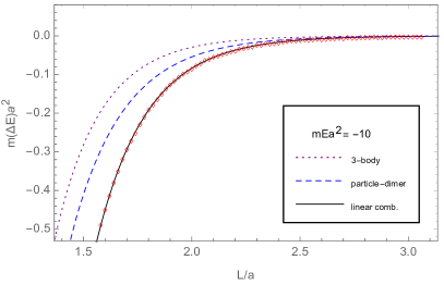
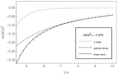
Figure 4: The two lowest energy levels from Fig. 3, corresponding to the bound states (red diamonds). We show the results of the fit by using the linear combination of Eqs. (40) and (41), as well as the individual contributions.

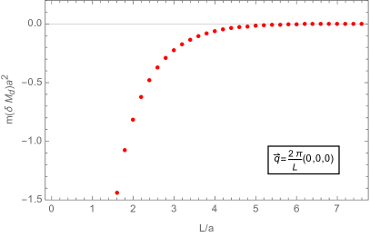
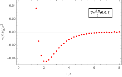
Figure 5: Finite-volume corrections $\delta M_{d}=M_{d}(L)-M_{d}(\infty)$ to the dimer mass in rest frame (left panel) as well as in the moving frame (right panel).

The volume dependence of the bound-state energy levels is shown in Fig. 4. We also show the fit to these energy levels by using the linear combination of Eqs. (40) and (41), treating $C$ and $C^{\prime}$ as free parameters, see Ref. pang1 . The fitting range for $L$ is chosen to be $[1.5,3.0]$ and $[4.6,10]$ in the left panel and right panel, respectively (it is necessary to choose different ranges because $\sqrt{\kappa^{2}-a^{-2}}\simeq 0.15\ll\kappa$). In addition, we display two different contributions to the final fit separately. Here one sees that the deeply bound state is well described by a mixture of the three-body bound state and a particle-dimer bound state with roughly equal weights in magnitude, whereas the shallow one is predominately a particle-dimer bound state. Moreover, we have checked that this picture stays robust, when one increases the lower range of the fit interval (moving this range to lower values of $L$ is not possible, because the suppressed contributions start to be sizable and the fit results are not stable anymore). Such a different behavior of two states can be understood as follows. First, we have seen before that the shallow bound state can be considered, to a good approximation, as a loosely bound state of a particle and a tightly bound dimer, since $\kappa^{2}-a^{-2}\ll\kappa^{2}$. At the same time, the deeply bound state can be considered as a predominately three-particle bound state based on the inequality $1/\kappa\ll a$. Since the inequality is fulfilled better for the shallow state than for the deep one, the particle-dimer component is stronger in the shallow state than the three-particle component in the deep one. So, the obtained results perfectly agree with our expectations.

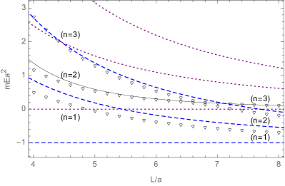
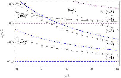
Figure 6: The three lowest-lying scattering states (black hearts) above threshold for different plot ranges. Each energy level is labeled by “(n=1,2,…)”. The result obtained using Eq. (43) is given by the black solid curve. The blue dashed curve shows the free particle-dimer states with back-to-back momenta $(0,0,0)$, $(0,0,1)$ and $(1,1,0)$, whereas the purple dotted lines denote the free three-particle states (the lowest level at $E=0$ corresponds to the threshold, where all three particles are at rest).

V.4 Scattering states

Let us start from the mass of an isolated dimer. In Fig. 5, left panel, we show the finite-volume corrections to the dimer mass in the rest frame, whereas in the right panel of the same figure, we show this quantity in the moving frame, when the CM of a dimer moves with a total momentum ${\bf k}=\frac{2\pi}{L}\,(0,0,1)$. The dimer mass is defined as

$$E_{2}(L)=M_{d}(L)+\frac{{\bf k}^{2}}{4m}\,,$$ (42)

where $E_{2}(L)$ is the energy level in the two-particle system (the solution of the Lüscher equation) and the rest mass of the dimer constituents is not included in $M_{d}(L)$. As seen from these figures, the correction is the largest in the rest frame. This directly follows from the Lüscher equation, since the finite volume corrections vanish exponentially at large $L$. The argument of the leading exponential is proportional to $k_{d}L$ with $k_{d}=\sqrt{\frac{1}{4}\,{\bf k}^{2}+mB_{2}}$ reaching its minimal value in the rest frame. Furthermore, since the energy of the particle-dimer state is given by the particle mass plus dimer mass plus the interaction energy between the particle and a dimer, one may expect that the corrections due to the $L$-dependence of the dimer mass are largest, when the dimer is in the rest frame.

Now let us return to Fig. 3 and try to interpret the states above threshold as the particle-dimer and three-particle scattering states. At large $L$, the energies of these states tend to $E=-1$ and $E=0$, respectively. In order to identify the levels at the intermediate values of $L$, let us use the expression for the volume-dependent shift of the three-particle ground-state energy level, obtained, e.g., in Refs. Beane:2007qr ; Sharpe:2017jej . Up to and including order $L^{-5}$, this expression contains only a single parameter $a$ and reads as

$$E=\frac{12\pi a}{L^{3}}-\frac{12a^{2}}{L^{4}}\,{\cal I}+\frac{12a^{3}}{\pi L^{5}}({\cal I}^{2}+{\cal J})+O(L^{-6})\,,~{}~{}~{}$$ (43)

where ${\cal I}\simeq-8.914$ and ${\cal J}\simeq 16.532$ are numerical constants. We now plot again the three lowest eigenvalues above threshold and confront them with the curve obtained from Eq. (43), see Fig. 6.

It is seen that, below $L\simeq 6.5$, the second level closely follows the prediction of the formula, so that it can be identified with the (shifted) ground state. After $L\simeq 6.5$ an avoided level crossing occurs, and it becomes clear that the third level has to be interpreted as the shifted ground state. The other two levels continue to move towards $E=-1$ and from now on should be interpreted as the particle-dimer scattering states. This is seen even better in the right panel of Fig. 6, which covers a larger interval in $L$. We observe more than one avoided level crossing in this figure.

Furthermore, as seen from these figures, the spectrum below the three-particle threshold closely follows the free particle-dimer energy levels (a small displacement is caused by interactions). However, at first glance, it seems that the counterpart of the ground-state level with the vanishing back-to-back momentum is missing.

In order to explain such a seemingly strange behavior, note that in the model we have a very shallow particle-dimer ground state with the energy $E=-1.016$, which “pushes” the next level up, close to the next free level with back-to-back momentum $(0,0,1)$. This can be seen in the following manner. One could choose the parameters of the model, so that the shallow bound state disappears. Choosing, for example, $H_{0}(\Lambda)=-1.353$ and the cutoff $\Lambda=20$, we get the energy of the deep bound state equal to $E=-5$, whereas the shallow bound state does not appear in the infinite-volume spectrum any more. The finite-volume energy spectrum for this case is shown in Fig. 7, where the level in the vicinity of the particle-dimer threshold is now a scattering state. Changing now all parameters of the model continuously, so that the lowest state just becomes the bound state again, will not change the position of the other levels very much, so in this case the level in the vicinity of the back-to-back momentum $(0,0,1)$ indeed corresponds to the lowest scattering state.

Albeit the intuitive interpretation of the energy levels, which was given above, is very transparent, we would like to stress that it is good for illustrative purposes only. Strictly speaking, in a finite volume one has only a spectrum that is determined by a full Hamiltonian of the system – no further labeling of the states can be justified rigorously.

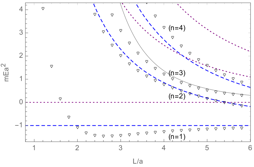
Figure 7: The same as in Fig. 6, but with a different value of the parameter $H_{0}(\Lambda)$, for which the shallow three-body bound state does not exist. The level that lies in the vicinity of the free particle-dimer threshold is a scattering state now.

VI Conclusion

The main results of our work can be summarized as follows:

• We have performed the projection of the three-particle quantization condition onto the different irreps of the octahedral group. As a result, the quantization condition partially diagonalizes – the different irreps do not talk to each other. Two alternative methods have been proposed. In both methods, the kernel that enters the quantization condition, instead of the spherical functions, is expanded in the basis vectors of various irreps of the octahedral group. The corresponding quantization conditions, given by Eqs. (26) and (37), are essentially equivalent.

• Using this method, the finite volume spectrum in the $A_{1}^{+}$ irrep was calculated, using a toy model corresponding to the leading order of the effective field theory for short range-interactions Bedaque:1998kg ; Bedaque:1998km . This model has interactions in the $S$-wave only. The results are very instructive. One directly sees that different bound states of the same model may have different nature (a three-particle bound state, a particle-dimer bound state, or something in between). Moreover, the scattering states cannot be uniquely interpreted as particle-dimer scattering states (in the infinite volume, these states appear in the elastic and rearrangement channels) and three-particle states (appearing in breakup reactions). At certain values of $L$, an “avoided level crossing” takes place when the different energy levels change their roles.

In the future, one may consider generalizations of this method in several directions. In particular, one may include interactions in higher partial waves, both in the two-body and three-body (particle-dimer) sector. One may consider moving frames. Finally, one may consider particles with spin, with the case of three nucleons being most interesting. Work in these directions is underway and will be discussed in future publications.

Acknowledgments

The authors thank U.-G. Meißner and E. Epelbaum for useful discussions. MD, MM, and AR acknowledge fruitful discussions with I. Aitchison, R. Briceño, Z. Davoudi, M. Hansen, A. Szczepaniak and S. Sharpe during the INT Workshop “Multi-Hadron Systems from Lattice QCD.” We acknowledge the support from the CRC 110 “Symmetries and the Emergence of Structure in QCD” (DFG grant no. TRR 110 and NSFC grant no. 11621131001) and the CRC 1245 “Nuclei: From Fundamental Interactions to Structure and Stars” (DFG grant no. SFB 1245) as well as support from the BMBF under contract no. 05P15RDFN1. This work was supported by the National Science Foundation under Grants No. PHY-1452055 and PHY-1415459 and by the U.S. Department of Energy, Office of Science, Office of Nuclear Physics under award number DE-SC001658 and under contract number DE-AC05-06OR23177. MM is thankful to the German Research Foundation (DFG) for the financial support, under the fellowship MA 7156/1-1, as well as to the George Washington University for the hospitality and inspiring environment. This research was also supported in part by Volkswagenstiftung under contract no. 93562 and by Shota Rustaveli National Science Foundation (SRNSF), grant no. DI-2016-26. MD, HWH, JYP, and AR thank the German Research Foundation (DFG) for support during the 2018 Hirschegg workshop “Multiparticle resonances in hadrons, nuclei, and ultracold gases” where this work was finalized.

Appendix A Matrices of the irreducible representations

In the following table, we quote the matrix representations of the five irreps $A_{1},A_{2},E,T_{1},T_{2}$. The numbering of the group elements $a=1,\ldots,24$ corresponds to table A.1 of Ref. Bernard:2008ax .

$a$	CC	$A_{1}$	$A_{2}$	$E$	$T_{1}$	$T_{2}$
1	$I$	$1$	$1$	$\begin{pmatrix}1&0\cr 0&1\end{pmatrix}$	$\begin{pmatrix}1&0&0\cr 0&1&0\cr 0&0&1\end{pmatrix}$	$\begin{pmatrix}1&0&0\cr 0&1&0\cr 0&0&1\end{pmatrix}$
2	$8C_{3}$	$1$	$1$	$\begin{pmatrix}-\frac{1}{2}&\frac{\sqrt{3}}{2}\cr-\frac{\sqrt{3}}{2}&-\frac{1}{2}\end{pmatrix}$	$\begin{pmatrix}0&1&0\cr 0&0&1\cr 1&0&0\end{pmatrix}$	$\begin{pmatrix}0&1&0\cr 0&0&1\cr 1&0&0\end{pmatrix}$
3		$1$	$1$	$\begin{pmatrix}-\frac{1}{2}&-\frac{\sqrt{3}}{2}\cr\frac{\sqrt{3}}{2}&-\frac{1}{2}\end{pmatrix}$	$\begin{pmatrix}0&0&1\cr 1&0&0\cr 0&1&0\end{pmatrix}$	$\begin{pmatrix}0&0&1\cr 1&0&0\cr 0&1&0\end{pmatrix}$
4		$1$	$1$	$\begin{pmatrix}-\frac{1}{2}&-\frac{\sqrt{3}}{2}\cr\frac{\sqrt{3}}{2}&-\frac{1}{2}\end{pmatrix}$	$\begin{pmatrix}0&0&-1\cr-1&0&0\cr 0&1&0\end{pmatrix}$	$\begin{pmatrix}0&0&-1\cr-1&0&0\cr 0&1&0\end{pmatrix}$
5		$1$	$1$	$\begin{pmatrix}-\frac{1}{2}&\frac{\sqrt{3}}{2}\cr-\frac{\sqrt{3}}{2}&-\frac{1}{2}\end{pmatrix}$	$\begin{pmatrix}0&-1&0\cr 0&0&1\cr-1&0&0\end{pmatrix}$	$\begin{pmatrix}0&-1&0\cr 0&0&1\cr-1&0&0\end{pmatrix}$
6		$1$	$1$	$\begin{pmatrix}-\frac{1}{2}&\frac{\sqrt{3}}{2}\cr-\frac{\sqrt{3}}{2}&-\frac{1}{2}\end{pmatrix}$	$\begin{pmatrix}0&1&0\cr 0&0&-1\cr-1&0&0\end{pmatrix}$	$\begin{pmatrix}0&1&0\cr 0&0&-1\cr-1&0&0\end{pmatrix}$
7		$1$	$1$	$\begin{pmatrix}-\frac{1}{2}&-\frac{\sqrt{3}}{2}\cr\frac{\sqrt{3}}{2}&-\frac{1}{2}\end{pmatrix}$	$\begin{pmatrix}0&0&-1\cr 1&0&0\cr 0&-1&0\end{pmatrix}$	$\begin{pmatrix}0&0&-1\cr 1&0&0\cr 0&-1&0\end{pmatrix}$
8		$1$	$1$	$\begin{pmatrix}-\frac{1}{2}&-\frac{\sqrt{3}}{2}\cr\frac{\sqrt{3}}{2}&-\frac{1}{2}\end{pmatrix}$	$\begin{pmatrix}0&0&1\cr-1&0&0\cr 0&-1&0\end{pmatrix}$	$\begin{pmatrix}0&0&1\cr-1&0&0\cr 0&-1&0\end{pmatrix}$
9		$1$	$1$	$\begin{pmatrix}-\frac{1}{2}&\frac{\sqrt{3}}{2}\cr-\frac{\sqrt{3}}{2}&-\frac{1}{2}\end{pmatrix}$	$\begin{pmatrix}0&-1&0\cr 0&0&-1\cr 1&0&0\end{pmatrix}$	$\begin{pmatrix}0&-1&0\cr 0&0&-1\cr 1&0&0\end{pmatrix}$
10	$6C_{4}$	$1$	$-1$	$\begin{pmatrix}-\frac{1}{2}&-\frac{\sqrt{3}}{2}\cr-\frac{\sqrt{3}}{2}&\frac{1}{2}\end{pmatrix}$	$\begin{pmatrix}1&0&0\cr 0&0&1\cr 0&-1&0\end{pmatrix}$	$\begin{pmatrix}-1&0&0\cr 0&0&-1\cr 0&1&0\end{pmatrix}$
11		$1$	$-1$	$\begin{pmatrix}-\frac{1}{2}&-\frac{\sqrt{3}}{2}\cr-\frac{\sqrt{3}}{2}&\frac{1}{2}\end{pmatrix}$	$\begin{pmatrix}1&0&0\cr 0&0&-1\cr 0&1&0\end{pmatrix}$	$\begin{pmatrix}-1&0&0\cr 0&0&1\cr 0&-1&0\end{pmatrix}$
12		$1$	$-1$	$\begin{pmatrix}-\frac{1}{2}&\frac{\sqrt{3}}{2}\cr\frac{\sqrt{3}}{2}&\frac{1}{2}\end{pmatrix}$	$\begin{pmatrix}0&0&-1\cr 0&1&0\cr 1&0&0\end{pmatrix}$	$\begin{pmatrix}0&0&1\cr 0&-1&0\cr-1&0&0\end{pmatrix}$

$a$	CC	$A_{1}$	$A_{2}$	$E$	$T_{1}$	$T_{2}$
13		$1$	$-1$	$\begin{pmatrix}-\frac{1}{2}&\frac{\sqrt{3}}{2}\cr\frac{\sqrt{3}}{2}&\frac{1}{2}\end{pmatrix}$	$\begin{pmatrix}0&0&1\cr 0&1&0\cr-1&0&0\end{pmatrix}$	$\begin{pmatrix}0&0&-1\cr 0&-1&0\cr 1&0&0\end{pmatrix}$
14		$1$	$-1$	$\begin{pmatrix}1&0\cr 0&-1\end{pmatrix}$	$\begin{pmatrix}0&1&0\cr-1&0&0\cr 0&0&1\end{pmatrix}$	$\begin{pmatrix}0&-1&0\cr 1&0&0\cr 0&0&-1\end{pmatrix}$
15		$1$	$-1$	$\begin{pmatrix}1&0\cr 0&-1\end{pmatrix}$	$\begin{pmatrix}0&-1&0\cr 1&0&0\cr 0&0&1\end{pmatrix}$	$\begin{pmatrix}0&1&0\cr-1&0&0\cr 0&0&-1\end{pmatrix}$
16	$6C_{2}^{\prime}$	$1$	$-1$	$\begin{pmatrix}-\frac{1}{2}&-\frac{\sqrt{3}}{2}\cr-\frac{\sqrt{3}}{2}&\frac{1}{2}\end{pmatrix}$	$\begin{pmatrix}-1&0&0\cr 0&0&1\cr 0&1&0\end{pmatrix}$	$\begin{pmatrix}1&0&0\cr 0&0&-1\cr 0&-1&0\end{pmatrix}$
17		$1$	$-1$	$\begin{pmatrix}-\frac{1}{2}&-\frac{\sqrt{3}}{2}\cr-\frac{\sqrt{3}}{2}&\frac{1}{2}\end{pmatrix}$	$\begin{pmatrix}-1&0&0\cr 0&0&-1\cr 0&-1&0\end{pmatrix}$	$\begin{pmatrix}1&0&0\cr 0&0&1\cr 0&1&0\end{pmatrix}$
18		$1$	$-1$	$\begin{pmatrix}1&0\cr 0&-1\end{pmatrix}$	$\begin{pmatrix}0&1&0\cr 1&0&0\cr 0&0&-1\end{pmatrix}$	$\begin{pmatrix}0&-1&0\cr-1&0&0\cr 0&0&1\end{pmatrix}$
19		$1$	$-1$	$\begin{pmatrix}1&0\cr 0&-1\end{pmatrix}$	$\begin{pmatrix}0&-1&0\cr-1&0&0\cr 0&0&-1\end{pmatrix}$	$\begin{pmatrix}0&1&0\cr 1&0&0\cr 0&0&1\end{pmatrix}$
20		$1$	$-1$	$\begin{pmatrix}-\frac{1}{2}&\frac{\sqrt{3}}{2}\cr\frac{\sqrt{3}}{2}&\frac{1}{2}\end{pmatrix}$	$\begin{pmatrix}0&0&1\cr 0&-1&0\cr 1&0&0\end{pmatrix}$	$\begin{pmatrix}0&0&-1\cr 0&1&0\cr-1&0&0\end{pmatrix}$
21		$1$	$-1$	$\begin{pmatrix}-\frac{1}{2}&\frac{\sqrt{3}}{2}\cr\frac{\sqrt{3}}{2}&\frac{1}{2}\end{pmatrix}$	$\begin{pmatrix}0&0&-1\cr 0&-1&0\cr-1&0&0\end{pmatrix}$	$\begin{pmatrix}0&0&1\cr 0&1&0\cr 1&0&0\end{pmatrix}$
22	$3C_{2}$	$1$	$1$	$\begin{pmatrix}1&0\cr 0&1\end{pmatrix}$	$\begin{pmatrix}1&0&0\cr 0&-1&0\cr 0&0&-1\end{pmatrix}$	$\begin{pmatrix}1&0&0\cr 0&-1&0\cr 0&0&-1\end{pmatrix}$
23		$1$	$1$	$\begin{pmatrix}1&0\cr 0&1\end{pmatrix}$	$\begin{pmatrix}-1&0&0\cr 0&1&0\cr 0&0&-1\end{pmatrix}$	$\begin{pmatrix}-1&0&0\cr 0&1&0\cr 0&0&-1\end{pmatrix}$
24		$1$	$1$	$\begin{pmatrix}1&0\cr 0&1\end{pmatrix}$	$\begin{pmatrix}-1&0&0\cr 0&-1&0\cr 0&0&1\end{pmatrix}$	$\begin{pmatrix}-1&0&0\cr 0&-1&0\cr 0&0&1\end{pmatrix}$

Table 1: Matrix representations of the irreps of the octahedral group (pure rotations). “CC“ denotes the conjugacy class, and $a=1,..,24$ index the group elements.

Appendix B Linear independent sets of cubic harmonics

Maximal sets of linearly independent cubic harmonics for $\ell\leq 9$ as determined by the procedure described in Section. IV for the corresponding shell types.

Shell type	$\vartheta$	Set
$(000)$	$1$	$X_{0}^{A_{1}^{+}11}$ [t]
$(00b)$	$6$	$X_{0}^{A_{1}^{+}11},X_{2}^{E^{+}11},X_{2}^{E^{+}12},X_{1}^{T_{1}^{-}11},X_{1}^{T_{1}^{-}12},X_{1}^{T_{1}^{-}13}$ [t]
$(0aa)$	$12$	$X_{0}^{A_{1}^{+}11},X_{2}^{E^{+}11},X_{2}^{E^{+}12},X_{1}^{T_{1}^{-}11},X_{1}^{T_{1}^{-}12},X_{1}^{T_{1}^{-}13},X_{2}^{T_{2}^{+}11},X_{2}^{T_{2}^{+}12},X_{2}^{T_{2}^{+}13},X_{3}^{T_{2}^{-}11},X_{3}^{T_{2}^{-}12},X_{3}^{T_{2}^{-}13}$ [t]
$(0bc)$	$24$	$X_{0}^{A_{1}^{+}11},X_{6}^{A_{2}^{+}11},X_{2}^{E^{+}11},X_{2}^{E^{+}12},X_{4}^{E^{+}11},X_{4}^{E^{+}12},X_{4}^{T_{1}^{+}11},X_{4}^{T_{1}^{+}12},X_{4}^{T_{1}^{+}13},X_{1}^{T_{1}^{-}11},X_{1}^{T_{1}^{-}12},X_{1}^{T_{1}^{-}13},$[t]
		$X_{3}^{T_{1}^{-}11},X_{3}^{T_{1}^{-}12},X_{3}^{T_{1}^{-}13},X_{2}^{T_{2}^{+}11},X_{2}^{T_{2}^{+}12},X_{2}^{T_{2}^{+}13},X_{3}^{T_{2}^{-}11},X_{3}^{T_{2}^{-}12},X_{3}^{T_{2}^{-}13},X_{5}^{T_{2}^{-}11},X_{5}^{T_{2}^{-}12},X_{5}^{T_{2}^{-}13}$
$(bbb)$	$8$	$X_{0}^{A_{1}^{+}11},X_{3}^{A_{2}^{-}11},X_{1}^{T_{1}^{-}11},X_{1}^{T_{1}^{-}12},X_{1}^{T_{1}^{-}13},X_{2}^{T_{2}^{+}11},X_{2}^{T_{2}^{+}12},X_{2}^{T_{2}^{+}13}$ [t]
$(bbc)$	24	$X_{0}^{A_{1}^{+}11},X_{3}^{A_{2}^{-}11},X_{2}^{E^{+}11},X_{2}^{E^{+}12},X_{5}^{E^{-}11},X_{5}^{E^{-}12},X_{4}^{T_{1}^{+}11},X_{4}^{T_{1}^{+}12},X_{4}^{T_{1}^{+}13},X_{1}^{T_{1}^{-}11},X_{1}^{T_{1}^{-}12},X_{1}^{T_{1}^{-}13},$ [t]
		$X_{3}^{T_{1}^{-}11},X_{3}^{T_{1}^{-}12},X_{3}^{T_{1}^{-}13},X_{2}^{T_{2}^{+}11},X_{2}^{T_{2}^{+}12},X_{2}^{T_{2}^{+}13},X_{4}^{T_{2}^{+}11},X_{4}^{T_{2}^{+}12},X_{4}^{T_{2}^{+}13},X_{3}^{T_{2}^{-}11},X_{3}^{T_{2}^{-}12},X_{3}^{T_{2}^{-}13}$
$(bcd)$	$48$	$X_{0}^{A_{1}^{+}11},X_{9}^{A_{1}^{-}11},X_{6}^{A_{2}^{+}11},X_{3}^{A_{2}^{-}11},X_{2}^{E^{+}11},X_{2}^{E^{+}12},X_{4}^{E^{+}11},X_{4}^{E^{+}12},X_{5}^{E^{-}11},X_{5}^{E^{-}12},X_{7}^{E^{-}11},X_{7}^{E^{-}12},$ [t]
		$X_{4}^{T_{1}^{+}11},X_{4}^{T_{1}^{+}12},X_{4}^{T_{1}^{+}13},X_{6}^{T_{1}^{+}11},X_{6}^{T_{1}^{+}12},X_{6}^{T_{1}^{+}13},X_{8}^{T_{1}^{+}21},X_{8}^{T_{1}^{+}22},X_{8}^{T_{1}^{+}23},X_{1}^{T_{1}^{-}11},X_{1}^{T_{1}^{-}12},$
		$X_{1}^{T_{1}^{-}13},X_{3}^{T_{1}^{-}11},X_{3}^{T_{1}^{-}12},X_{3}^{T_{1}^{-}13},X_{5}^{T_{1}^{-}11},X_{5}^{T_{1}^{-}12},X_{5}^{T_{1}^{-}13},X_{2}^{T_{2}^{+}11},X_{2}^{T_{2}^{+}12},X_{2}^{T_{2}^{+}13},X_{4}^{T_{2}^{+}11},$
		$X_{4}^{T_{2}^{+}12},X_{4}^{T_{2}^{+}13},X_{6}^{T_{2}^{+}11},X_{6}^{T_{2}^{+}12},X_{6}^{T_{2}^{+}13},X_{3}^{T_{2}^{-}11},X_{3}^{T_{2}^{-}12},X_{3}^{T_{2}^{-}13},X_{5}^{T_{2}^{-}11},X_{5}^{T_{2}^{-}12},X_{5}^{T_{2}^{-}13},$
		$X_{7}^{T_{2}^{-}21},X_{7}^{T_{2}^{-}22},X_{7}^{T_{2}^{-}23}$

Table 2: Full sets of cubic harmonics $X_{\ell}^{\Gamma\nu\alpha}$ with $\ell\leq 9$, contributing to the basis vectors on a shell of a given type. Here $\vartheta$ denotes the multiplicity, i.e., the number of points (and therefore of basis vectors) on a given shell.

References

- (1) M. Lüscher, Commun. Math. Phys. 105 (1986) 153.
- (2) M. Lüscher, Nucl. Phys. B 354 (1991) 531.
- (3) H.-W. Hammer, J.-Y. Pang and A. Rusetsky, JHEP 1709 (2017) 109, [arXiv:1706.07700].
- (4) H.-W. Hammer, J.-Y. Pang and A. Rusetsky, JHEP 1710 (2017) 115, [arXiv:1707.02176].
- (5) M. Mai and M. Döring, Eur. Phys. J. A 53 (2017) 240 [arXiv:1709.08222].
- (6) R. A. Briceño, M. T. Hansen and S. R. Sharpe, Phys. Rev. D 95 (2017) 074510 [arXiv:1701.07465 [hep-lat]].
- (7) P. Guo and V. Gasparian, arXiv:1709.08255 [hep-lat].
- (8) P. Guo and V. Gasparian, Phys. Lett. B 774 (2017) 441 [arXiv:1701.00438 [hep-lat]].
- (9) P. Guo, Phys. Rev. D 95 (2017) 054508 [arXiv:1607.03184 [hep-lat]].
- (10) M. T. Hansen and S. R. Sharpe, Phys. Rev. D 93 (2016) 096006 Erratum: [Phys. Rev. D 96 (2017) 039901] [arXiv:1602.00324 [hep-lat]].
- (11) M. T. Hansen and S. R. Sharpe, Phys. Rev. D 93 (2016) 014506 [arXiv:1509.07929 [hep-lat]].
- (12) M. T. Hansen and S. R. Sharpe, Phys. Rev. D 92 (2015) 114509 [arXiv:1504.04248 [hep-lat]].
- (13) U.-G. Meißner, G. Ríos and A. Rusetsky, Phys. Rev. Lett. 114 (2015) 091602 Erratum: [Phys. Rev. Lett. 117 (2016) 069902] [arXiv:1412.4969 [hep-lat]].
- (14) M. T. Hansen and S. R. Sharpe, Phys. Rev. D 90 (2014) 116003 [arXiv:1408.5933].
- (15) K. Polejaeva and A. Rusetsky, Eur. Phys. J. A 48 (2012) 67 [arXiv:1203.1241].
- (16) R. A. Briceño and Z. Davoudi, Phys. Rev. D 87 (2013) 094507 [arXiv:1212.3398].
- (17) L. Roca and E. Oset, Phys. Rev. D 85 (2012) 054507 [arXiv:1201.0438 [hep-lat]].
- (18) R. A. Briceño, J. J. Dudek and R. D. Young, arXiv:1706.06223 [hep-lat].
- (19) R. A. Briceño, Z. Davoudi and T. C. Luu, J. Phys. G 42 (2015) 023101 [arXiv:1406.5673 [hep-lat]].
- (20) S. Kreuzer and H.-W. Hammer, Phys. Lett. B 673 (2009) 260 [arXiv:0811.0159].
- (21) S. Kreuzer and H.-W. Hammer, Eur. Phys. J. A 43 (2010) 229 [arXiv:0910.2191].
- (22) S. Kreuzer and H.-W. Hammer, Phys. Lett. B 694 (2011) 424 [arXiv:1008.4499].
- (23) S. Kreuzer and H. W. Grießhammer, Eur. Phys. J. A 48 (2012) 93 [arXiv:1205.0277].
- (24) M. Jansen, H.-W. Hammer and Y. Jia, Phys. Rev. D 92 (2015) 114031 [arXiv:1505.04099 [hep-ph]].
- (25) S. Aoki, N. Ishii, T. Doi, Y. Ikeda and T. Inoue, Phys. Rev. D 88 (2013) 014036 [arXiv:1303.2210 [hep-lat]].
- (26) S. Bour, H.-W. Hammer, D. Lee and U.-G. Meißner, Phys. Rev. C 86 (2012) 034003 [arXiv:1206.1765 [nucl-th]].
- (27) S. Bour, S. König, D. Lee, H.-W. Hammer and U.-G. Meißner, Phys. Rev. D 84 (2011) 091503 [arXiv:1107.1272 [nucl-th]].
- (28) M. T. Hansen, H. B. Meyer and D. Robaina, Phys. Rev. D 96 (2017) 094513 [arXiv:1704.08993 [hep-lat]].
- (29) D. Agadjanov, M. Döring, M. Mai, U.-G. Meißner and A. Rusetsky, JHEP 1606 (2016) 043 [arXiv:1603.07205 [hep-lat]].
- (30) M. T. Hansen and S. R. Sharpe, Phys. Rev. D 95 (2017) 034501, [arXiv:1609.04317].
- (31) Y. Meng, C. Liu, U. G. Meißner and A. Rusetsky, arXiv:1712.08464 [hep-lat].
- (32) S. R. Beane, W. Detmold and M. J. Savage, Phys. Rev. D 76 (2007) 074507 [arXiv:0707.1670].
- (33) S. R. Sharpe, Phys. Rev. D 96 (2017) 054515, [arXiv:1707.04279].
- (34) E.W. Schmid and H. Ziegelmann, The Quantum Mechanical Three-Body Problem, Vieweg Tracts in Pure and Applied Physics Vol. 2, Pergamon Press (1974).
- (35) J. Golak et al., Eur. Phys. J. A 50 (2014) 177 [arXiv:1410.0756].
- (36) M. Lüscher, Commun. Math. Phys. 105 (1986) 153.
- (37) M. Döring, U.-G. Meißner, E. Oset and A. Rusetsky, Eur. Phys. J. A 48 (2012) 114 [arXiv:1205.4838].
- (38) P. F. Bedaque, H.-W. Hammer and U. van Kolck, Phys. Rev. Lett. 82 (1999) 463 [nucl-th/9809025].
- (39) P. F. Bedaque, H.-W. Hammer and U. van Kolck, Nucl. Phys. A 646 (1999) 444 [nucl-th/9811046].
- (40) P. F. Bedaque and H. W. Griesshammer, Nucl. Phys. A 671 (2000) 357 [nucl-th/9907077].
- (41) M. Mai, B. Hu, M. Döring, A. Pilloni and A. Szczepaniak, Eur. Phys. J. A 53 (2017) 177 [arXiv:1706.06118].
- (42) V. Bernard, M. Lage, U.-G. Meißner and A. Rusetsky, JHEP 0808 (2008) 024, [arXiv:0806.4495].
- (43) M. Göckeler, R. Horsley, M. Lage, U.-G. Meißner, P. E. L. Rakow, A. Rusetsky, G. Schierholz and J. M. Zanotti, Phys. Rev. D 86 (2012) 094513, [arXiv:1206.4141].
- (44) V. Efimov, Nucl. Phys. A 210 (1973) 157.
- (45) M. Lüscher, Commun. Math. Phys. 104 (1986) 177.
- (46) S. König and D. Lee, arXiv:1701.00279 [hep-lat].