Optimal data fitting: a moment approach

Abstract

We propose a moment relaxation for two problems, the separation and covering problems with semi-algebraic sets generated by a polynomial of degree $d$. We show that (a) the optimal value of the relaxation finitely converges to the optimal value of the original problem, when the moment order $r$ increases and (b) after performing some small perturbation of the original problem, convergence can be achieved with $r=d$. We further provide a practical iterative algorithm that is computationally tractable for large datasets and present encouraging computational results.

1 Introduction

Data fitting problems have long been very useful in many different application areas. A well-known problem is the problem of finding the minimum-volume ellipsoid in $n$-dimensional space $\mathbb{R}^{n}$ containing all points that belong to a given finite set $S\subset\mathbb{R}^{n}$. This minimum-volume covering ellipsoid problem is important in the area of robust statistics, data mining, and cluster analysis (see e.g. Sun and Freund [17] and the recent book by M. Todd [19]). Pattern separation as described in Calafiore [4] is another related problem, in which an ellipsoid that separates a set of points $S_{1}$ from another set of points $S_{2}$ needs to be found under some appropriate optimality criteria such as minimum volume or minimum distance error.

These problems have been studied for a long time. The minimum-volume covering ellipsoid (MVCE) problem was discussed by John [9] in 1948. This problem has been modeled as a convex optimization problem with linear matrix inequalities (LMI) and solved by interior-point methods (IPM) in Vandenberghe et al. [21], Sun and Freund [17] and Magnani et al. [14]. In particular, the ”dual-reduced-Newton” algorithm presented in [17] combines interior-point and active-set methods allowing one to efficiently compute the MVCE of moderately large datasets (in dimension $n=30$ and dataset with $30000$ points, it takes a few seconds on a personal laptop). The recent survey by Todd [19] provides more details on algorithms depending on the size of the datasets and the dimension. In particular, for huge-scale problems ($n=500$ and and datasets with $500000$ points), the Wolfe-Atwood algorithm [18] is the only one able to compute the MVCE.

The problem of pattern separation via ellipsoids was studied by Rosen [15] and Barnes [2]. Glineur [6] has proposed some methods to solve this problem with different optimality criteria via conic programming. Although efficient algorithms are already available, they could become computationally intractable if the cardinality of datasets is large. In addition, different semi-algebraic sets other than ellipsoidal sets could be considered for these data fitting problems. Note that for complicated clusters as in Figure 1, it will be impossible in general to separate two datasets with ellipsoids.

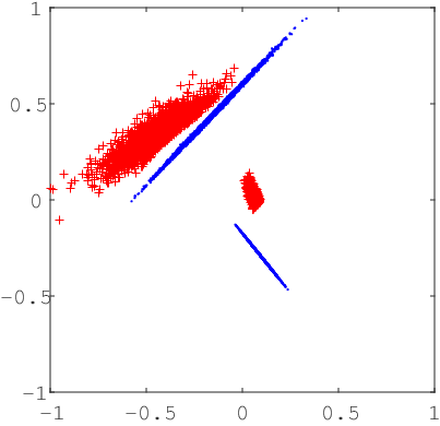
Figure 1: Two datasets $S_{1}$ (blue) and $S_{2}$ (red) non separable with ellipsoids.

This was our motivation to approximate such datasets with the level set of a polynomial $\theta$ of a priori fixed degree $d$, possibly greater than 2. Given two datasets $S_{1}$ and $S_{2}$, the superlevel (resp. sublevel) set of $\theta$ should contain $S_{1}$ (resp. $S_{2}$). Interestingly, this approach can also be used for minimum-volume covering problems when $S_{2}=\emptyset$. However for very large datasets, this may not be competitive with dedicated algorithms, such as the ones presented in [19].

With $\boldsymbol{\gamma}=(\gamma_{1},\dots,\gamma_{n})\in\mathbb{N}^{n}$, let us note $\boldsymbol{x}^{\boldsymbol{\gamma}}\stackrel{{\scriptstyle\bigtriangleup}}{{=}}x_{1}^{\gamma_{1}}\,\cdots\,x_{n}^{\gamma_{n}}$ and $|\boldsymbol{\gamma}|\stackrel{{\scriptstyle\bigtriangleup}}{{=}}\gamma_{1}+\dots+\gamma_{n}$. One possible approach to find the coefficients of the above-mentioned polynomial $\theta=\sum_{\boldsymbol{\gamma}}\theta_{\boldsymbol{\gamma}}\boldsymbol{x}^{\boldsymbol{\gamma}}$ is to solve the following linear problem (LP):

$$\left[\begin{array}[]{lrr}\inf&\sum_{|\boldsymbol{\gamma}|\leq d}|\theta_{\boldsymbol{\gamma}}|&\\ \mathop{\rm s.t.}&\theta(\boldsymbol{x})\geq 0,&\forall\boldsymbol{x}\in S_{1},\\ &-\theta({\boldsymbol{x}})\geq 0,&\forall{\boldsymbol{x}}\in S_{2},\\ &\theta\in\mathbb{R}[\boldsymbol{x}],&\deg\theta=d.\end{array}\right]$$ (1)

When $\theta$ has degree $d$, this LP has $\binom{n+d}{n}$ variables and $|S_{1}|+|S_{2}|$ constraints on the vector of coefficients of the polynomial $\theta$. The variables of LP (1) are the coefficients $(\theta_{\gamma})_{|\gamma|\leq d}$ of the polynomial $\theta$.
Given a feasible solution $\theta$ of LP (1), the superlevel (resp. sublevel) set of $\theta$ contains $S_{1}$ (resp. $S_{2}$). Therefore, we choose the $\ell_{1}$-norm of the coefficient vector of $\theta$ for the objective function, in order to minimize the volume of the level-sets of $\theta$.
This LP may become ill-conditioned whenever several points from the clusters are close to each other. The reason is that in this case the LP has almost redundant inequality constraints. We performed practical experiments with several LP solvers (Gurobi [7], SDPT3 [20], Mosek [1], SeDuMi [16]), which all include a pre-processing step to remove nearly dependent constraints (see [20, § 1.3.5]).

By solving LP (1), we were able to separate datasets of small size (less than $10^{2}$ points). For various randomly generated datasets of larger size, such as the datasets $S_{1}$ and $S_{2}$ (with $10^{5}$ points) depicted in Figure 1, we experienced numerical issues either with the algorithm implemented in the LP solvers.
Another drawback of this LP formulation is that it cannot tackle all data fitting applications considered in the present study, including minimum-volume covering ellipsoids.

Contributions and Paper Outline

In this paper we propose a common methodology for these data fitting problems and in particular its extension to general basic semi-algebraic sets (more general than ellipsoids) based on a moment approach. This methodology is based on the moment-SOS approach and has the distinguishing feature to not individualize each point of the two clouds of data points, that is, we do not incorporate positivity constraints of the type $\pm\theta(\boldsymbol{x}_{i})\geq 0$ for each point of the cloud. More precisely:

1. In Section 2, we propose a moment relaxation for these data fitting problems with basic semi-algebraic sets $\Omega=\{{\boldsymbol{x}}\in\mathbb{R}^{n}:\theta({\boldsymbol{x}})\geq 0\}$, where $\theta\in\mathbb{R}[{\boldsymbol{x}}]$ is a polynomial with a priori fixed degree $d$. One main advantage is to avoid considering $|S_{1}|+|S_{2}|$ constraints (i.e. avoids individualizing each point). The information of each dataset $|S_{i}|$ is collected in a localizing matrix $M_{r}(\theta\boldsymbol{y}^{i})$ associated to an empirical measure $\mu^{i}$ supported on $|S_{i}|$ (and where $y^{i}$ is a finite vector of moments associated with $\mu^{i}$). In our case, we perform a smoothing thanks to the two LMIs: $M_{r}(\theta\boldsymbol{y}^{1})\succeq 0$ (associated to $S_{1}$) and $M_{r}(\theta\boldsymbol{y}^{2})\preceq 0$ (associated to $S_{2}$), with $r\in\mathbb{N}$. When the first (resp. second) condition is satisfied for all $r$, this is actually equivalent to the nonnegativity of $\theta$ (resp. $-\theta$) on the support of $\mu^{1}$ (resp. $\mu^{2}$) (see [11]). We show in Proposition 1 that the optimal value of the relaxation converges in finitely many steps to the optimal value of the original problem, when the moment order $r$ increases. The key idea of our approach is that, instead of imposing a constraint for each point in the dataset, we require that the support of any probability measure $\mu$ that is generated on the dataset is contained in $\Omega$. Using powerful results from the theory of moments, we may replace all membership constraints by two Linear Matrix Inequality (LMI) constraints of size $\binom{n+r}{r}$. Hence for 3D-datasets the size of each of the two LMIs is $O(r^{3}/6)$ (and so for a quartic polynomial ($r=4$), the size of each LMI is only $\binom{3+4}{3}=35$).

2. In Section 3, we show the following result: If $\max[|S_{1}|,|S_{2}|]=s$ and the degree $d$ of the polynomial $\theta$ is such that $\binom{n+d}{n}\geq s$, then finite convergence occurs at step $r=d$, generically. This genericity condition can be ensured after performing some arbitrary small perturbation of the original problem. The possible drawbacks of this method is that for large size clusters, the size of the localizing matrices grows rapidly, leading to LMIs which are expensive to solve. Therefore to handle large datasets in practice we combine the above approach with a heuristic inspired from results on semi-infinite optimization by Ben-Tal et al. [3].

3. In Section 4, we provide a practical iterative algorithm based on the results of Section 3 for these data fitting problems that is computationally tractable for datasets with a very large number of points. The corresponding method is an iterative procedure where the degree of the polynomial is fixed in advance (typically $r=2$ or $r=4$) and where we solve a moment relaxation with measures supported on subsets of the initial cluster. Even though this algorithm does not always converge, it happens to be very efficient in practice. We present encouraging computational results of cluster separation with up to $10^{5}$ points, either with ellipsoid or quartic level sets.

2 Moment Relaxations

2.1 Problem Formulation

With $\boldsymbol{x}=(x_{1},\dots,x_{n})$, consider a polynomial $\theta\in\mathbb{R}[\boldsymbol{x}]$ of degree at most $d$: $\theta(\boldsymbol{x})=\sum_{\boldsymbol{\gamma}\in\mathbb{N}^{n}:|\boldsymbol{\gamma}\rvert\leq d}\theta_{\boldsymbol{\gamma}}\boldsymbol{x}^{\boldsymbol{\gamma}}$. Letting $\boldsymbol{\theta}=\{\theta_{\boldsymbol{\gamma}}:\boldsymbol{\gamma}\in\mathbb{N}^{n},|\boldsymbol{\gamma}\rvert\leq d\}$ be the coefficient vector of $\theta$, $\boldsymbol{\theta}\in\mathbb{R}^{t}$, where $t=\binom{n+d}{d}$ and $\Theta\subset\mathbb{R}^{t}$, we obtain a family of semi-algebraic sets $\Omega_{\theta}=\{{\boldsymbol{x}}\in\mathbb{R}^{n}:\theta({\boldsymbol{x}})\geq 0\}$ for $\theta\in\Theta$. The problem of separating a finite dataset $S_{1}\subset\mathbb{R}^{n}$ from another finite dataset $S_{2}\subset\mathbb{R}^{n}$ with one of these semi-algebraic sets can be written as follows:

$${{\cal P}}^{s}\quad\left[\begin{array}[]{llrr}\tau^{s}=&\inf&f(\boldsymbol{\theta})&\\ &\mathop{\rm s.t.}&\theta(\boldsymbol{x})\geq 0,&\forall\boldsymbol{x}\in S_{1},\\ &&-\theta({\boldsymbol{x}})\geq 0,&\forall{\boldsymbol{x}}\in S_{2},\\ &&\boldsymbol{\theta}\in\Theta,\end{array}\right]$$ (2)

where $f$ is an optimality criterion and $\tau^{s}$ is the optimal value of ${\cal P}^{s}$.

If we only consider one dataset $S$, then we can formulate the problem of covering $S$ with the best semi-algebraic set $\Omega_{\theta}$ with respect to optimality criterion $f$ as follows:

$${{\cal P}}^{c}\quad\left[\begin{array}[]{llrr}\tau^{c}=&\inf&f(\boldsymbol{\theta})&\\ &\mathop{\rm s.t.}&\theta(\boldsymbol{x})\geq 0,&\forall\boldsymbol{x}\in S,\\ &&\boldsymbol{\theta}\in\Theta.\end{array}\right]$$ (3)

If $f$ is the volume function of ellipsoids and $\theta$ is a quadratic function that generates ellipsoidal sets, then the pattern separation via ellipsoids and minimum-volume covering ellipsoid problems are obtained respectively from these two general problems. Thus, for $r=1$, we consider $f=\log\det\boldsymbol{Q}^{-1}$ with $\boldsymbol{Q}$ being a positive definite matrix of size $n$ and a separating polynomial $\theta(\boldsymbol{x})=-\boldsymbol{x}^{\prime}\boldsymbol{Q}\boldsymbol{x}+\boldsymbol{b}^{\prime}\boldsymbol{x}+c$. When using level sets of polynomials with higher degree $2r$, we consider the same cost function $f=\log\det\boldsymbol{Q}^{-1}$ with a positive definite matrix $\boldsymbol{Q}$ of size $\binom{n+r-1}{n}$ and a separating polynomial $\theta(\boldsymbol{x}):=-v_{r}(\boldsymbol{x})^{\prime}\boldsymbol{Q}v_{r}(\boldsymbol{x})+\boldsymbol{b}^{\prime}v_{r}(\boldsymbol{x})+c$, where $v_{r}(\boldsymbol{x})$ is the vector of degree-$r$ monomials, i.e. $(x_{1}^{r},x_{1}^{r-1}x_{2},\dots,x_{n}^{r})$. Note that we can also consider the more general separating polynomial $\theta(\boldsymbol{x}):=1-w_{r}(\boldsymbol{x})^{\prime}\boldsymbol{Q}w_{r}(\boldsymbol{x})$, with $w_{r}(\boldsymbol{x})$ being the vector of all monomials with degree at most $r$ (See Section 4.2 and Section 4.3 for more practical details).

Since the covering problem is a special case of the separation problem ($S_{2}=\emptyset$), we focus on the latter problem in the following sections.

2.2 Moment Formulation

We now investigate the application of the moment-SOS approach (see Henrion [8], Lasserre [10], and the references therein) to Problem (2). Let $\mu^{i}$ be a probability measure generated on $S_{i}$, $i=1,2$,

$$\mu^{i}:=\sum_{\boldsymbol{x}\in S_{i}}\mu^{i}_{\boldsymbol{x}}\delta_{\boldsymbol{x}},$$ (4)

where $\delta_{\boldsymbol{x}}$ denotes the Dirac measure at $\boldsymbol{x}$, $\sum_{\boldsymbol{x}\in S_{i}}\mu^{i}_{\boldsymbol{x}}=1$, and $\mu^{i}_{\boldsymbol{x}}\geq 0$ for all $\boldsymbol{x}\in S_{i}$, $i=1,2$. For example, the uniform probability measure $\mu^{i}$ generated on $S_{i}$ has $\mu^{i}_{\boldsymbol{x}}=1/|S_{i}\rvert$ for all $\boldsymbol{x}\in S_{i}$.

All the moments $\boldsymbol{y}^{i}=\left\{y^{i}_{\boldsymbol{\alpha}}\right\}$ of $\mu^{i}$ are calculated as follows:

$$y^{i}_{\boldsymbol{\alpha}}=\int\boldsymbol{x}^{\boldsymbol{\alpha}}\mathrm{d}\mu^{i}=\sum_{\boldsymbol{x}\in S_{i}}\mu^{i}_{\boldsymbol{x}}\boldsymbol{x}^{\boldsymbol{\alpha}},\quad\boldsymbol{\alpha}\in\mathbb{N}^{n}.$$ (5)

For any nonnegative integer $r$, the $r$-moment matrix associated with $\mu^{i}$ (or equivalently, with $\boldsymbol{y}^{i}$) $M_{r}(\mu^{i})\equiv M_{r}(\boldsymbol{y}^{i})$ is a matrix of size $\binom{n+r}{r}$. Its rows and columns are indexed in the canonical basis $\left\{\boldsymbol{x}^{\boldsymbol{\alpha}}\right\}$ of $\mathbb{R}[\boldsymbol{x}]$, and its elements are defined as follows:

$$M_{r}(\boldsymbol{y}^{i})(\boldsymbol{\alpha},\boldsymbol{\beta})=y^{i}_{\boldsymbol{\alpha}+\boldsymbol{\beta}},\quad\boldsymbol{\alpha},\boldsymbol{\beta}\in\mathbb{N}^{n},|\boldsymbol{\alpha}\rvert,|\boldsymbol{\beta}\rvert\leq r.$$ (6)

Similarly, given $\theta\in\mathbb{R}[\boldsymbol{x}]$, the localizing matrix $M_{r}(\boldsymbol{\theta}\boldsymbol{y}^{i})$ associated with $\boldsymbol{y}^{i}$ and $\theta$ is defined by

$$M_{r}(\boldsymbol{\theta}\boldsymbol{y}^{i})(\boldsymbol{\alpha},\boldsymbol{\beta}):=\sum_{\boldsymbol{\gamma}\in\mathbb{N}^{n}}\theta_{\boldsymbol{\gamma}}y^{i}_{\boldsymbol{\alpha}+\boldsymbol{\beta}+\boldsymbol{\gamma}},\quad\boldsymbol{\alpha},\boldsymbol{\beta}\in\mathbb{N}^{n},|\boldsymbol{\alpha}\rvert,|\boldsymbol{\beta}\rvert\leq r,$$ (7)

where $\boldsymbol{\theta}=\left\{\theta_{\boldsymbol{\gamma}}\right\}$ is the vector of coefficients of $\theta$ in the canonical basis $\left\{\boldsymbol{x}^{\boldsymbol{\alpha}}\right\}$.

If we define the matrix $M_{r}^{\boldsymbol{\gamma}}(\boldsymbol{y}^{i})$ with elements

$$M_{r}^{\boldsymbol{\gamma}}(\boldsymbol{y}^{i})(\boldsymbol{\alpha},\boldsymbol{\beta})=y^{i}_{\boldsymbol{\alpha}+\boldsymbol{\beta}+\boldsymbol{\gamma}},\quad\boldsymbol{\alpha},\boldsymbol{\beta},\boldsymbol{\gamma}\in\mathbb{N}^{n},|\boldsymbol{\alpha}\rvert,|\boldsymbol{\beta}\rvert\leq r,$$

then the localizing matrix can be expressed as $M_{r}(\boldsymbol{\theta}\boldsymbol{y}^{i})=\sum_{\boldsymbol{\gamma}\in\mathbb{N}^{n}}\theta_{\boldsymbol{\gamma}}M_{r}^{\boldsymbol{\gamma}}(\boldsymbol{y}^{i})$.

Note that for every polynomial $f\in\mathbb{R}[\boldsymbol{x}]$ of degree at most $r$ with its vector of coefficients denoted by $\boldsymbol{f}=\left\{f_{\boldsymbol{\gamma}}\right\}$, we have:

$$\langle\boldsymbol{f},M_{r}(\boldsymbol{\theta}\boldsymbol{y}^{i})\boldsymbol{f}\rangle=\int\theta f^{2}\mathrm{d}\mu^{i}.$$ (8)

This property shows that necessarily, $M_{r}(\boldsymbol{\theta}\boldsymbol{y}^{i})\succeq\boldsymbol{0}$, whenever $\mu^{i}$ has its support contained in the level set $\left\{\boldsymbol{x}\in\mathbb{R}^{n}:\theta(\boldsymbol{x})\geq 0\right\}$. Therefore, if we replace all membership constraints in Problem ${\cal P}^{s}$ by two LMI constraints $M_{r}(\boldsymbol{\theta}\boldsymbol{y}^{1})\succeq 0$ and $M_{r}(-\boldsymbol{\theta}\boldsymbol{y}^{2})\succeq 0$, we obtain a relaxation of Problem ${\cal P}^{s}$:

$${{\cal P}}^{s}_{r}(\boldsymbol{y}^{1},\mbox{\boldmath$y$}^{2})\quad\left[\begin{array}[]{lrl}\tau^{s}_{r}(\boldsymbol{y}^{1},\mbox{\boldmath$y$}^{2})=&\inf&f(\boldsymbol{\theta})\\ &\mathop{\rm s.t.}&M_{r}(\boldsymbol{\theta}\boldsymbol{y}^{1})\succeq\boldsymbol{0}\\ &&M_{r}(-\boldsymbol{\theta}\boldsymbol{y}^{2})\succeq\boldsymbol{0}\\ &&\boldsymbol{\theta}\in\Theta,\end{array}\right]$$ (9)

with optimal value denoted by $\tau^{s}_{r}(\boldsymbol{y}^{1},\mbox{\boldmath$y$}^{2})$. We emphasize that ${{\cal P}}^{s}_{r}(\boldsymbol{y}^{1},\mbox{\boldmath$y$}^{2})$ depends on $\boldsymbol{y}^{1}$ and $\boldsymbol{y}^{2}$, the respective moment sequences of the two measures $\mu^{1}$ and $\mu^{2}$, that are both fixed beforehand. Next, we prove that the convergence of $\tau^{s}_{r}(\boldsymbol{y}^{1},\mbox{\boldmath$y$}^{2})$ to $\tau^{s}$ occurs under mild properties of $\mu^{1}$ and $\mu^{2}$.

2.3 Convergence as the number of moments increases

Compared to ${\cal P}^{s}$, the data of $S_{1}$ and $S_{2}$ are aggregated into the vector $\boldsymbol{y}^{1}$ and $\mbox{\boldmath$y$}^{2}$ used in ${{\cal P}}^{s}_{r}(\boldsymbol{y}^{1},\mbox{\boldmath$y$}^{2})$. Both problems have exactly the same variables, but

1. Problem ${\cal P}^{s}$ has $|S_{1}\rvert+|S_{2}\rvert$ linear constraints, whereas

2. Problem ${{\cal P}}^{s}_{r}(\boldsymbol{y})$ has two LMI constraints $M_{r}(\boldsymbol{\theta}\boldsymbol{y}^{1})\succeq 0$ and $M_{r}(-\boldsymbol{\theta}\boldsymbol{y}^{2})\succeq 0$ with matrix size $\binom{n+r}{r}$.

If $r$ is not too large, solving ${{\cal P}}^{s}_{r}(\boldsymbol{y})$ is preferable to solving ${\cal P}^{s}$, especially if $|S_{1}\rvert+|S_{2}\rvert$ is large. It is natural to ask how good this moment relaxation could be as compared to the original problem and which value of $r$ we have to use to obtain a strong lower bound. In this section, let us assume that fixed probability measures $\mu^{i}$ generated on $S_{i}$, $i=1,2$, are selected; for example, the uniform probability measures as mentioned in the previous section.

Proposition 1

Let $\theta\in\mathbb{R}[{\boldsymbol{x}}]$, and let ${\cal P}^{s}$, ${{\cal P}}^{s}_{r}(\boldsymbol{y}^{1},\mbox{\boldmath$y$}^{2})$, $r\in\mathbb{N}$ be as in (2) and (9) respectively. Then:

$$\tau^{s}_{r}(\boldsymbol{y}^{1},\mbox{\boldmath$y$}^{2})\leq\tau^{s}_{r+1}(\boldsymbol{y}^{1},\mbox{\boldmath$y$}^{2}),\quad\mbox{and}\quad\tau^{s}_{r}(\boldsymbol{y}^{1},\mbox{\boldmath$y$}^{2})\leq\tau^{s},\quad\forall r\in\mathbb{N},$$

where $\tau^{s}$ and $\tau^{s}_{r}(\boldsymbol{y}^{1},\mbox{\boldmath$y$}^{2})$ are optimal values of ${\cal P}^{s}$ and ${{\cal P}}^{s}_{r}(\boldsymbol{y}^{1},\mbox{\boldmath$y$}^{2})$ respectively.

Proof. For every $\boldsymbol{\gamma}\in\mathbb{N}^{n}$, $M_{r}^{\boldsymbol{\gamma}}(\boldsymbol{y}^{i})$ is the north-west corner square sub-matrix with size $\binom{n+r}{r}$ of $M_{r+1}^{\boldsymbol{\gamma}}(\boldsymbol{y}^{i})$, $i=1,2$. This follows directly from the definition of the matrix $M_{r}^{\boldsymbol{\gamma}}(\boldsymbol{y}^{i})$.

Since $M_{r}(\boldsymbol{\theta}\boldsymbol{y}^{1})=\sum_{\boldsymbol{\gamma}\in\mathbb{N}^{n}}\theta_{\boldsymbol{\gamma}}M_{r}^{\boldsymbol{\gamma}}(\boldsymbol{y}^{1})$ for all $r$, $M_{r}(\boldsymbol{\theta}\boldsymbol{y}^{1})$ is also a north-west corner square submatrix of $M_{r+1}(\boldsymbol{\theta}\boldsymbol{y}^{1})$. This implies that if $M_{r+1}(\boldsymbol{\theta}\boldsymbol{y}^{1})\succeq\boldsymbol{0}$, then $M_{r}(\boldsymbol{\theta}\boldsymbol{y}^{1})\succeq\boldsymbol{0}$. Similar arguments can be applied for $M_{r}(-\boldsymbol{\theta}\boldsymbol{y}^{2})$ and $M_{r+1}(-\boldsymbol{\theta}\boldsymbol{y}^{2})$. Thus, any feasible solution of ${{\cal P}}^{s}_{r+1}(\boldsymbol{y}^{1},\mbox{\boldmath$y$}^{2})$ is feasible for ${{\cal P}}^{s}_{r}(\boldsymbol{y}^{1},\mbox{\boldmath$y$}^{2})$. So we have:

$$\tau^{s}_{r}(\boldsymbol{y}^{1},\mbox{\boldmath$y$}^{2})\leq\tau^{s}_{r+1}(\boldsymbol{y}^{1},\mbox{\boldmath$y$}^{2}),\quad\forall r\in\mathbb{N}.$$

Similarly, any feasible solution of ${\cal P}^{s}$ is feasible for ${{\cal P}}^{s}_{r}(\boldsymbol{y}^{1},\mbox{\boldmath$y$}^{2})$. Indeed, if $\boldsymbol{\theta}$ is feasible for ${\cal P}^{s}$ then we have $\theta(\boldsymbol{x})\geq 0$ for all $\boldsymbol{x}\in S_{1}$ and $\theta({\boldsymbol{x}})\leq 0$ for all ${\boldsymbol{x}}\in S_{2}$. Therefore, the probability measures $\mu^{1}$ and $\mu^{2}$ defined in (4) have their supports contained in the level set $\left\{\boldsymbol{x}\in\mathbb{R}^{n}:\theta(\boldsymbol{x})\geq 0\right\}$ and $\left\{\boldsymbol{x}\in\mathbb{R}^{n}:\theta(\boldsymbol{x})\leq 0\right\}$ respectively. In view of (8), we have $M_{r}(\boldsymbol{\theta}\boldsymbol{y}^{1})\succeq\boldsymbol{0}$ and $M_{r}(-\boldsymbol{\theta}\boldsymbol{y}^{2})\succeq\boldsymbol{0}$. This proves that $\boldsymbol{\theta}$ is feasible for ${{\cal P}}^{s}_{r}(\boldsymbol{y}^{1},\mbox{\boldmath$y$}^{2})$ with any $r\in\mathbb{N}$. Thus, $\tau^{s}_{r}(\boldsymbol{y}^{1},\mbox{\boldmath$y$}^{2})\leq\tau^{s},\quad\forall r\in\mathbb{N}.$ $\square$

We next show that if $\mu^{i}$ is supported on the whole set $S_{i}$, $i=1,2$, then the optimal values $\left\{\tau^{s}_{r}(\boldsymbol{y}^{1},\mbox{\boldmath$y$}^{2})\right\}$ converges to $\tau^{s}$, when $r$ increases and the convergence is finite. The statement is formally stated and proved as follows:

Theorem 1

Let ${\cal P}^{s}$, $\mu^{i}$ and ${{\cal P}}^{s}_{r}(\boldsymbol{y}^{1},\mbox{\boldmath$y$}^{2})$, $r\in\mathbb{N}$ be as in (2), (4) and (9), respectively. If $\mu^{i}_{\boldsymbol{x}}>0$ for all $\boldsymbol{x}\in S_{i}$, $i=1,2$, then

$$\tau^{s}_{r}(\boldsymbol{y}^{1},\mbox{\boldmath$y$}^{2})\uparrow\tau^{s}\quad\mbox{ as $r$ increases,}$$

and the convergence is finite.

Proof. From Proposition 1, we have $\tau^{s}_{r}(\boldsymbol{y}^{1},\mbox{\boldmath$y$}^{2})\leq\tau^{s},\quad\forall r\in\mathbb{N}.$ In addition, as $\mu^{i}$ in (4) is finitely supported, its moment matrix $M_{r}(\boldsymbol{y}^{i})$ defined in (6) with $\boldsymbol{y}^{i}$ as in (5) has finite rank. That is, there exists $r^{i}_{0}\in\mathbb{N}$ such that

$$\mbox{rank}(M_{r}(\boldsymbol{y}^{i}))=\mbox{rank}(M_{r^{i}_{0}}(\boldsymbol{y})),\quad\forall r\geq r^{i}_{0}.$$

In other words, $M_{r}(\boldsymbol{y}^{i})$ is a flat extension of $M_{r_{0}}(\boldsymbol{y}^{i})$ for all $r\geq r^{i}_{0}$ (see Curto and Fialkow [5] for more details).

Now, let $r_{0}:=\max\{r^{1}_{0},r^{2}_{0}\}$ and let $\boldsymbol{\theta}$ be an arbitrary $\epsilon$-optimal solution of ${{\cal P}}^{s}_{r_{0}}(\boldsymbol{y}^{1},\mbox{\boldmath$y$}^{2})$, $\epsilon>0$, i.e., $f(\boldsymbol{\theta})\leq\tau^{s}_{r_{0}}(\boldsymbol{y}^{1},\mbox{\boldmath$y$}^{2})+\epsilon$. As $M_{r_{0}}(\boldsymbol{\theta}\,\boldsymbol{y}^{i})\succeq\boldsymbol{0}$ and since $M_{r_{0}+\frac{\deg\theta}{2}}(\boldsymbol{y}^{i})\succeq\boldsymbol{0}$, we may invoke Theorem 1.6 in [5] and deduce that $\mu^{1}$ has its support contained in the level set $\left\{\boldsymbol{x}\in\mathbb{R}^{n}:\theta(\boldsymbol{x})\geq 0\right\}$. Similarly, $\mu^{2}$ has its support contained in the level set $\left\{\boldsymbol{x}\in\mathbb{R}^{n}:\theta(\boldsymbol{x})\leq 0\right\}$. This implies that $\theta(\boldsymbol{x})\geq 0$ for all $\boldsymbol{x}\in S_{1}$ and $\theta(\boldsymbol{x})\leq 0$ for all $\boldsymbol{x}\in S_{2}$ because $\mu^{i}$ is supported on the whole set $S_{i}$ ($\mu^{i}_{\boldsymbol{x}}>0$ for all $\boldsymbol{x}\in S_{i}$). Thus, $\boldsymbol{\theta}$ is feasible for ${\cal P}^{s}$ and $\tau^{s}\leq f(\boldsymbol{\theta})\leq\tau^{s}_{r_{0}}(\boldsymbol{y}^{1},\mbox{\boldmath$y$}^{2})+\epsilon$. We then have

$$\tau^{s}_{r_{0}}(\boldsymbol{y}^{1},\mbox{\boldmath$y$}^{2})\leq\tau^{s}\leq\tau^{s}_{r_{0}}(\boldsymbol{y}^{1},\mbox{\boldmath$y$}^{2})+\epsilon.$$

As $\epsilon>0$ was arbitrary, $\tau^{s}_{r_{0}}(\boldsymbol{y}^{1},\mbox{\boldmath$y$}^{2})=\tau^{s}$. Since from Proposition 1 $\tau^{s}_{r}(\boldsymbol{y}^{1},\mbox{\boldmath$y$}^{2})$ is monotone and bounded, we obtain that $\tau^{s}_{r}(\boldsymbol{y}^{1},\mbox{\boldmath$y$}^{2})\uparrow\tau^{s}$ and the convergence is finite. $\square$

Theorem 1 provides the rationale for solving ${{\cal P}}^{s}_{r}(\boldsymbol{y}^{1},\mbox{\boldmath$y$}^{2})$ instead of ${\cal P}^{s}$. However, despite the finite convergence we do not know how large the value of $r_{0}$ could be. In the next section, we will discuss how to select appropriate values $r$ for Problem ${{\cal P}}^{s}_{r}(\boldsymbol{y}^{1},\mbox{\boldmath$y$}^{2})$.

3 Convergence of Measures

In this section, we analyze how the genericity of the datasets $S_{1}\subset\mathbb{R}^{n}$ and $S_{2}\subset\mathbb{R}^{n}$ affects the convergence of ${{\cal P}}^{s}_{r}(\boldsymbol{y}^{1},\mbox{\boldmath$y$}^{2})$.

Definition 1 ($r$-genericity)

We say that $S$ is said “$r$-generic” when $S$ does not belong to the level set of any polynomial of degree at most $r$.

We next investigate how different (and much “smaller”) atomic probability measures can be selected to yield optimality.

3.1 Convergence in Measure

As mentioned in the previous section, $\tau^{s}_{r}(\boldsymbol{y}^{1},\mbox{\boldmath$y$}^{2})$ converges to $\tau^{s}$ as $r$ increases, and there exists an index $r_{0}$ such that $\tau^{s}_{r_{0}}(\boldsymbol{y}^{1},\mbox{\boldmath$y$}^{2})=\tau^{s}$. As for several other problems reformulated with moment relaxations, no explicit value for the relaxation order $r_{0}$ is available in general. We investigate next the dependence of $r_{0}$ on $|S_{1}\rvert$ and $|S_{2}\rvert$ and show that under certain rank conditions, we will have $\tau^{s}_{r}(\boldsymbol{y}^{1},\mbox{\boldmath$y$}^{2})=\tau^{s}$ for any probability measures $\mu^{i}$ supported on the whole set $S_{i}$, $i=1,2$.

Proposition 2

Let ${\cal P}^{s}$, $\mu^{i}$, and ${{\cal P}}^{s}_{r}(\boldsymbol{y}^{1},\mbox{\boldmath$y$}^{2})$ be as in (2), (4), and (9), respectively. Assume that $|S_{i}\rvert=\binom{n+r}{r}$, $S_{i}$ is $r$-generic (in the sense of Definition 1), and $\mu^{i}_{\boldsymbol{x}}>0$ for all $\boldsymbol{x}\in S_{i}$ for $i=1,2$. Then the following holds:

$$|S_{i}\rvert=\mbox{rank}\,(M_{r}(\boldsymbol{y}^{i}))\quad\text{and}\quad\tau^{s}_{r}(\boldsymbol{y}^{1},\mbox{\boldmath$y$}^{2})=\tau^{s}\,.$$

Proof. Note that $M_{r}(\boldsymbol{y}^{i})$ is an $\binom{n+r}{r}\times\binom{n+r}{r}$ matrix and the probability measure $\mu^{i}$ is supported on the whole set $S_{i}$, with $|S_{i}\rvert=\binom{n+r}{r}$, i.e. $\mu^{i}$ is an $|S_{i}\rvert$-atomic measure. For $i=1,2$, we first show that the rank of the matrix $M_{r}(\boldsymbol{y}^{i})$ is maximal, i.e. $\mbox{rank}\,(M_{r}(\boldsymbol{y}^{i}))=\binom{n+r}{r}=|S_{i}\rvert$. For each $x\in S_{i}$, we denote by $\zeta_{x}:=(x^{\alpha})_{|\alpha|\leq r}$ the moment sequence associated to the Dirac measure at $x$. Note that $M_{r}(\boldsymbol{y}^{i})=\sum_{x\in S_{i}}\mu_{x}\,\zeta_{x}\zeta_{x}^{T}=GG^{T}$, where $G$ is the $\binom{n+r}{r}\times\binom{n+r}{r}$ matrix whose columns are the vectors $\sqrt{\mu_{x}}\zeta_{x}$. We show that $G$ is invertible. Indeed, if $Gz=0$ for some vector $(z_{\alpha})_{|\alpha|\leq r}$, then one has $\sqrt{\mu_{x}}\sum_{|\alpha|\leq r}z_{\alpha}x^{\alpha}=0$, for all $x\in S_{i}$. Thus, $S_{i}$ belongs to the level set $\{\boldsymbol{x}:g_{i}(\boldsymbol{x})=0\}$ of the polynomial $g_{i}$ (of degree at most $r$) with vector of coefficients $z$. This contradicts our assumption and therefore necessarily $z=0$, which implies that $G$ is non singular and which in turn implies that $M_{r}(\boldsymbol{y}^{i})$ is also invertible. Hence, one has $|S_{i}\rvert=\mbox{rank}\,(M_{r}(\boldsymbol{y}^{i}))$.

Then according to Laurent [12, Lemma 2.7], there exist $|S_{i}\rvert$ interpolation polynomials $f_{j}\in\mathbb{R}[\boldsymbol{x}]$ of degree at most $r$, $j=1,\ldots,|S_{i}\rvert$, such that

$$f_{j}(\boldsymbol{x}(k))=\left\{\begin{array}[]{lr}0,&j\neq k,\\ 1,&j=k,\end{array}\right.\quad\forall j,k=1,\ldots,|S_{i}\rvert.$$

Now, let $\boldsymbol{\theta}$ be an arbitrary $\epsilon$-optimal solution of ${{\cal P}}^{s}_{r}(\boldsymbol{y}^{1},\mbox{\boldmath$y$}^{2})$, $\epsilon>0$. As $\boldsymbol{\theta}$ is feasible for ${{\cal P}}^{s}_{r}(\boldsymbol{y}^{1},\mbox{\boldmath$y$}^{2})$, $M_{r}(\boldsymbol{\theta}\boldsymbol{y}^{1})\succeq\boldsymbol{0}$, $M_{r}(-\boldsymbol{\theta}\boldsymbol{y}^{2})\succeq\boldsymbol{0}$ and $f(\boldsymbol{\theta})\leq\tau^{s}_{r}(\boldsymbol{y}^{1},\mbox{\boldmath$y$}^{2})+\epsilon$. For every $j=1,\ldots,|S_{1}\rvert$, we have:

$$\langle\boldsymbol{f}_{j},M_{r}(\boldsymbol{\theta}\boldsymbol{y}^{1})\boldsymbol{f}_{j}\rangle\geq 0,$$

where $\boldsymbol{f}_{j}$ is the vector of coefficients of the polynomial $f_{j}$. Then Eq. (8) implies that

$$\int\theta f_{j}^{2}\mathrm{d}\mu^{1}\geq 0\Leftrightarrow\mu^{1}_{\boldsymbol{x}(j)}\theta(\boldsymbol{x}_{j})\geq 0.$$

Since $\mu^{1}_{\boldsymbol{x}}>0$ for all $\boldsymbol{x}\in S_{1}$, we obtain $\theta(\boldsymbol{x}(j))\geq 0$ for all $j=1,\ldots,|S_{1}\rvert$. Similarly, we also obtain $\theta(\boldsymbol{x}(j))\leq 0$ for all $j=1,\ldots,|S_{2}\rvert$. Thus, $\boldsymbol{\theta}$ is feasible for ${\cal P}^{s}$ and $\tau^{s}\leq f(\boldsymbol{\theta})\leq\tau^{s}_{r}(\boldsymbol{y}^{1},\mbox{\boldmath$y$}^{2})+\epsilon$. Combining with results from Proposition 1, we have

$$\tau^{s}_{r}(\boldsymbol{y}^{1},\mbox{\boldmath$y$}^{2})\leq\tau^{s}\leq\tau^{s}_{r}(\boldsymbol{y}^{1},\mbox{\boldmath$y$}^{2})+\epsilon.$$

As $\epsilon>0$ was arbitrarily chosen, we obtain $\tau^{s}_{r}(\boldsymbol{y}^{1},\mbox{\boldmath$y$}^{2})=\tau^{s}$. $\square$

Remark 1

In the case when $|S_{i}\rvert=\binom{n+r}{r}$, the assumption that $S_{i}$ is $r$-generic (in the sense of Definition 1) holds. Indeed, the points of $S_{i}$ in general position impose $\binom{n+r}{r}$ independent linear conditions, which is the maximal number of coefficients of a polynomial of degree $r$.

If we select $r_{0}=\min\left\{r\in\mathbb{N}:\binom{n+r}{r}\geq\max\{|S_{1}\rvert,|S_{2}\rvert\}\right\}$, the condition $|S_{i}\rvert=\binom{n+r_{0}}{r_{0}}$, $i=1,2$, does not hold in general, thus Proposition 2 cannot be directly applied. However, we can apply the following perturbation algorithm to the initial datasets $S_{1}$ and $S_{2}$ to ensure that the rank condition generically holds:

Perturbation Algorithm

• For $i=1,2$, replicate $(r_{0}-|S_{i}\rvert)$ times an arbitrary point of $S_{i}$ to obtain a new dataset $S_{i}^{\prime}$ with $|S_{i}^{\prime}|=\binom{n+r}{r}$.

• Choose an arbitrary small $\epsilon>0$, fixed. For $i=1,2$ and each $x\in S_{i}^{\prime}$, generate a random unit vector $\tilde{u}\in\mathbb{S}^{n-1}$ from the rotation-invariant probability distribution on $\mathbb{S}^{n-1}$ and replace $\boldsymbol{x}$ with $\boldsymbol{x}+\epsilon\tilde{u}\in B(\boldsymbol{x},\epsilon)$ (where $B(\boldsymbol{x};\epsilon)$ is the ball centered at $\boldsymbol{x}$ and with radius $\epsilon$). The perturbed dataset $\tilde{S}_{i}$ is the set of all randomly generated vectors $\tilde{\boldsymbol{x}}$.

• Output $\tilde{S}_{1}$ and $\tilde{S}_{2}$.

After applying this algorithm, the rank condition generically holds and one can apply Proposition 2 to the perturbed datasets $\tilde{S}_{1}$ and $\tilde{S}_{2}$.

Although the result of Proposition 2 is interesting, it is not very useful for practical algorithms. Problem ${{\cal P}}_{r_{0}}^{s}({\boldsymbol{y}}^{1},{\boldsymbol{y}}^{2})$ has only two LMI constraints but its matrix size is at least $\max\{|S_{1}\rvert,|S_{2}\rvert\}$, which could be very large. It means that Problem ${{\cal P}}_{r}^{s}({\boldsymbol{y}}^{1},{\boldsymbol{y}}^{2})$ is still computationally difficult to solve, when $|S_{1}\rvert$ or $|S_{2}\rvert$ is large. However in the next section, we use Proposition 2 and show that we can generically find appropriate probability measures ${\mu}^{i}$ such that ${\tau}^{s}_{r}({\boldsymbol{y}}^{1},{\boldsymbol{y}}^{2})={\tau}^{s}$ for $r$ as small as $d$, which is the degree of the polynomial $\theta$.

3.2 Optimal Measure

The probability measure $\mu^{i}$ is defined in (4) as $\mu^{i}=\sum_{\boldsymbol{x}\in S_{i}}\mu^{i}_{\boldsymbol{x}}\delta_{\boldsymbol{x}}$ with $\sum_{\boldsymbol{x}\in S_{i}}\mu^{i}_{\boldsymbol{x}}=1$ and $\mu^{i}_{\boldsymbol{x}}\geq 0$ for all $\boldsymbol{x}\in S_{i}$. Let $\boldsymbol{\mu}^{i}=\left(\mu^{i}_{\boldsymbol{x}_{1}},\ldots,\mu^{i}_{\boldsymbol{x}_{|S\rvert_{i}}}\right)$, we have, $\boldsymbol{\mu}^{i}\in M_{|S_{i}\rvert}$, where $M_{|S_{i}\rvert}=\left\{\boldsymbol{x}\in\mathbb{R}^{|S_{i}\rvert}_{+}:\sum_{i=1}^{|S_{i}\rvert}x_{i}=1\right\}$. Each probability measure $\mu^{i}$ can then be represented equivalently by a vector $\boldsymbol{\mu}^{i}\in M_{|S_{i}\rvert}$. Thus, the optimal value of Problem ${{\cal P}}^{s}_{r}(\boldsymbol{y}^{1},\mbox{\boldmath$y$}^{2})$ can also be expressed as $\tau^{s}_{r}(\boldsymbol{\mu}^{1},\boldsymbol{\mu}^{2})\equiv\tau^{s}_{r}(\boldsymbol{y}^{1},\mbox{\boldmath$y$}^{2})$.

Clearly, we can form infinitely many moment relaxations from different probability measures generated on $S_{i}$ as above. But the question is then: which pair of probability measures yields the best relaxation? With $r$ fixed, consider the following problem:

$${{\cal P}}^{s}_{r}\quad\left[\rho^{s}_{r}=\sup_{\boldsymbol{\mu}^{i}\in M_{|S_{i}\rvert}}\tau^{s}_{r}(\boldsymbol{\mu}^{1},\boldsymbol{\mu}^{2})\right]\,,$$ (10)

where $\rho^{s}_{r}$ is the optimal value of ${{\cal P}}^{s}_{r}$. We then immediately have the following result

Proposition 3

Let ${\cal P}^{s}$ and ${{\cal P}}^{s}_{r}$ be as in (2) and (10) respectively. Then $\rho^{s}_{r}\leq\tau^{s}.$

Proof. From Proposition 1, we have $\tau^{s}_{r}(\boldsymbol{\mu}^{1},\boldsymbol{\mu}^{2})\equiv\tau^{s}_{r}(\boldsymbol{y}^{1},\mbox{\boldmath$y$}^{2})\leq\tau^{s}$ for all $\boldsymbol{\mu}^{i}\in M_{|S_{i}\rvert}$, $i=1,2$. Therefore $\sup_{\boldsymbol{\mu}^{i}\in M_{|S_{i}\rvert}}\tau^{s}_{r}(\boldsymbol{\mu}^{1},\boldsymbol{\mu}^{2})\leq\tau^{s}$.

$\square$

We are interested in finding the minimum value of the moment order $r$ that turns the above inequality into an equality. We observe that in view of the convexity of $f$ and $\Theta$, the optimal solution of ${\cal P}^{s}$ depends only on some (possibly small) subsets of $S_{1}\subset\mathbb{R}^{n}$ and $S_{2}\subset\mathbb{R}^{n}$. Indeed, the following result was proved by Ben-Tal et al. [3]:

Theorem 2

[Ben-Tal et al. [3, Theorem 3.1]] Consider the problem

$${{\cal P}}\quad\left[\begin{array}[]{rl}\inf&f(\boldsymbol{\theta})\\ \mathop{\rm s.t.}&g_{k}(\boldsymbol{\theta},{\boldsymbol{x}})\leq 0,\quad{\boldsymbol{x}}\in S_{k},\quad k=1,\ldots,m,\\ &\boldsymbol{\theta}\in\Theta,\end{array}\right]$$

and assume that

1. the set $\Theta\subset\mathbb{R}^{t}$ is convex with non empty interior,

2. the function $f$ is continuous and convex on $\Theta$,

3. the function $g_{k}$ is continuous in ${\boldsymbol{x}}$,

4. for all $k\in\mathbb{N}$, the function $g_{k}$ is continuous and convex in $\boldsymbol{\theta}$ on $\Theta$ and the set $\{\boldsymbol{\theta}:g_{k}(\boldsymbol{\theta},{\boldsymbol{x}})<0\}$ is open, for each ${\boldsymbol{x}}\in S_{k}$,

5. (Slater condition) the set $\{\boldsymbol{\theta}\in\mathbb{R}^{t}:g_{k}(\boldsymbol{\theta},{\boldsymbol{x}})<0,{\boldsymbol{x}}\in S_{k},k=1,\ldots,m\}$ is nonempty.

Let $\boldsymbol{\theta}^{*}$ be a feasible solution of ${\cal P}$, $S_{k}(\boldsymbol{\theta}^{*})=\{{\boldsymbol{x}}\in S_{k}:g_{k}(\boldsymbol{\theta}^{*},{\boldsymbol{x}})=0\}$, and $K^{*}=\{k:S_{k}(\boldsymbol{\theta}^{*})\neq\emptyset\}$. Then $\boldsymbol{\theta}^{*}$ is an optimal solution of ${\cal P}$ if and only if there is a set $S^{*}\subset\cup_{k\in K^{*}}S_{k}(\boldsymbol{\theta}^{*})$ with at most $t$ elements such that $\boldsymbol{\theta}^{*}$ is the optimal solution of the problem:

$${{\cal P}}^{*}\quad\left[\begin{array}[]{rl}\inf&f(\boldsymbol{\theta})\\ \mathop{\rm s.t.}&g_{k}(\boldsymbol{\theta},{\boldsymbol{x}})\leq 0,\quad{\boldsymbol{x}}\in S^{*}\cap S_{k},\quad k\in K^{*},\\ &\boldsymbol{\theta}\in\Theta.\end{array}\right]$$

Using Theorem 2 with $g_{1}(\boldsymbol{\theta},{\boldsymbol{x}}):=-\boldsymbol{\theta}({\boldsymbol{x}})$ and $g_{2}(\boldsymbol{\theta},{\boldsymbol{x}}):=\boldsymbol{\theta}({\boldsymbol{x}})$, we see that our initial problem of separating the two datasets $S_{1}$ and $S_{2}$ boils down to separating the two datasets $S^{*}\cap S_{1}$ and $S^{*}\cap S_{2}$, of smaller size, bounded by $\binom{n+d}{n}$. Our aim is then to apply Proposition 2 in order to solve exactly this equivalent problem. To do so, we need the two initial datasets $S_{1}$ and $S_{2}$ to fulfill genericity conditions, which are slightly stronger than the one stated in Definition 1.

Theorem 3

Let ${\cal P}^{s}$, ${{\cal P}}^{s}_{r}$ be defined as in (2), (10) respectively, whose variables are the coefficients of a degree $d$ polynomial $\theta\in\Theta$. Assume that $\Theta$ is convex, $f$ is convex on $\Theta$, Slater condition is satisfied and that each subset of $S_{i}$ of size less than $\binom{n+d}{n}$ for $i=1,2$ is $d$-generic (in the sense of Definition 1). If ${{\cal P}}^{s}$ is solvable, then the following generically holds for all $r\geq d$:

$${\rho}^{s}_{r}={\tau}^{s}.$$

Proof. Let us consider the separation problem ${{\cal P}}^{s}$. In our context $g_{k}(\theta,\boldsymbol{x})=\sum_{\alpha}\theta_{\alpha}\boldsymbol{x}^{\alpha}$ and therefore $g_{k}$ satisfies (A3) and (A4). As ${{\cal P}}^{s}$ is solvable with optimal solution $\boldsymbol{\theta}^{*}$, we can apply the results of Theorem 2 with $t=\binom{n+d}{n}$. Thus, there exists a set $S^{*}$ such that $\boldsymbol{\theta}^{*}$ is the optimal solution of the reduced problem ${{\cal P}}^{*}$ associated to ${{\cal P}}^{s}$:

$${{\cal P}}^{*}\quad\left[\begin{array}[]{rl}\inf&f(\boldsymbol{\theta})\\ \mathop{\rm s.t.}&\theta({\boldsymbol{x}})\geq 0,\quad{\boldsymbol{x}}\in S^{*}\cap S_{1},\\ &\theta({\boldsymbol{x}})\leq 0,\quad{\boldsymbol{x}}\in S^{*}\cap S_{2},\\ &\boldsymbol{\theta}\in\Theta.\end{array}\right]$$

In general, the cardinal $c_{i}$ of $S^{*}\cap S_{i}$ will be strictly less than $t=\binom{n+d}{n}$ and we cannot apply Proposition 2 to the reduced problem ${{\cal P}}^{*}$. However, we can modify ${{\cal P}}^{*}$ by considering two sets $S_{i}^{*}$ of cardinal $t$, obtained after adding $t-c_{i}$ points of $S_{i}$ to $S^{*}\cap S_{i}$, for $i=1,2$. Since $S^{*}\cap S_{i}\subseteq S_{i}^{*}$ for $i=1,2$, if $\theta$ (resp. $-\theta$) is nonnegative on $S_{1}^{*}$ (resp. $S_{2}^{*}$) then it is also nonnegative on $S^{*}\cap S_{1}$ (resp. $S^{*}\cap S_{2}$). In other words, it is sufficient to separate $S_{1}^{*}$ and $S_{2}^{*}$ with the level set of $\theta$ since the same level set separates $S^{*}\cap S_{1}$ and $S^{*}\cap S_{2}$ (and thus $S_{1}$ et $S_{2}$).

This leads to the following problem:

$${{\cal P}}^{s}(S_{1}^{*},S_{2}^{*})\quad\left[\begin{array}[]{lrl}{\tau}^{s}(S_{1}^{*},S_{2}^{*})=&\inf&f(\boldsymbol{\theta})\\ &\mathop{\rm s.t.}&\theta({\boldsymbol{x}})\geq 0,\quad{\boldsymbol{x}}\in S_{1}^{*},\\ &&\theta({\boldsymbol{x}})\leq 0,\quad{\boldsymbol{x}}\in S_{2}^{*},\\ &&\boldsymbol{\theta}\in\Theta.\end{array}\right]$$

where ${\tau}^{s}(S_{1}^{*},S_{2}^{*})$ denotes the optimal value of ${{\cal P}}^{s}(S_{1}^{*},S_{2}^{*})$. In other words, the problem of separating $S_{1}$ and $S_{2}$ is equivalent to the problem of separating two datasets $S_{1}^{*}$ and $S_{2}^{*}$ of smaller size (but of course, $S_{1}^{*}$ and $S_{2}^{*}$ are not known in advance).

Note that ${\tau}^{s}(S_{1}^{*},S_{2}^{*})$ is equal to the optimal value of ${{\cal P}}^{*}$, which is also equal to the optimal value of ${{\cal P}}^{s}$. Both optimal values are reached at the same $\boldsymbol{\theta}^{*}$ and $\tau^{s}=\tau^{s}(S_{1}^{*},S_{2}^{*})$.

Then we choose probability measures ${\mu}^{i}_{0}$ (with the moment vector ${\boldsymbol{y}}^{i}_{0}$) supported exactly on the whole set $S_{i}^{*}$, that is, for all $\boldsymbol{x}\in S_{i}$, $\mu^{i}_{\boldsymbol{x}}>0$ if and only if $\boldsymbol{x}\in S_{i}^{*}$, for $i=1,2$. Clearly, $\boldsymbol{\mu}^{i}_{0}\in M_{|{S}_{i}\rvert}$, for $i=1,2$, thus ${\tau}^{s}_{d}({\boldsymbol{\mu}}^{1}_{0},{\boldsymbol{\mu}}^{2}_{0})\leq\rho^{s}_{d}$.

The probability measure ${\mu}^{i}_{0}$ is supported on the whole set $S_{i}^{*}$, for $i=1,2$, thus ${\cal P}^{s}_{d}({\boldsymbol{y}}^{1}_{0},{\boldsymbol{y}}^{2}_{0})$ is also a moment relaxation of Problem ${{\cal P}}^{s}(S_{1}^{*},S_{2}^{*})$. Thanks to the $d$-genericity assumptions on all subsets of $S_{1}$ and $S_{2}$, the two datasets $S_{1}^{*}$ and $S_{2}^{*}$ do not belong to the level set of any polynomial of degree at most $d$. Therefore, we can apply the result from Proposition 2, yielding ${\tau}^{s}_{d}({\boldsymbol{y}}^{1}_{0},{\boldsymbol{y}}^{2}_{0})\equiv\tau^{s}_{d}({\boldsymbol{\mu}}^{1}_{0},{\boldsymbol{\mu}}^{2}_{0})={\tau}^{s}(S_{1}^{*},S_{2}^{*})$ since the points of $S_{i}^{*}$ are in generic position and $|S_{i}^{*}|=t=\binom{n+d}{n}$, for $i=1,2$.

From Proposition 3, we have ${\rho}^{s}_{d}\leq{\rho}^{s}_{r}\leq{\tau}^{s}$ for all $r\geq d$. From these inequalities and equalities, we have: ${\tau}^{s}={\tau}^{s}(S_{1}^{*},S_{2}^{*})={\tau}^{s}_{d}({\boldsymbol{\mu}}^{1}_{0},{\boldsymbol{\mu}}^{2}_{0})\leq{\rho}^{s}_{d}\leq{\rho}^{s}_{r}\leq{\tau}^{s}$, for all $r\geq d$.

$\square$

Note that after running the perturbation algorithm from § 3.1, the $d$-genericity assumption of Theorem 3 is fulfilled for all subsets of $S_{1}$ and $S_{2}$. The result is that, with $r$ as small as $d$, some moment relaxation ${{\cal P}}^{s}_{r}({\boldsymbol{y}}^{1},{\boldsymbol{y}}^{2})$ is equivalent to Problem ${{\cal P}}^{s}$, given that the appropriate probability measures $\mu^{1}$ and $\mu^{2}$ are used. These appropriate measures are uniformly supported on two datasets $S_{1}^{*}$ and $S_{2}^{*}$ of smaller size. If we would know these smaller datasets, we could easily separate $S_{1}$ and $S_{2}$ by solving the equivalent reduced problem. Notice that for instance with $d=4$ and $n=3$ ($2$ clouds of 3D-points), one is left with $35\times 35$ psd matrices only (with $2D$-points then the size of each matrix drops to $15\times 15$).

The goal of the next section is to propose a practical iterative algorithm to compute separating candidate polynomials.

4 Practical Algorithm

4.1 Algorithm

The key question is how to select the optimal probability measures for Problem ${{\cal P}}^{s}_{r}$. The proof of Theorem 3 suggests that in order to find the optimal probability measures, we need to find the set of points $S_{i}^{*}$, for $i=1,2$, that defines the optimal solution of Problem ${{\cal P}}^{s}$. We propose a practical iterative algorithm to select the optimal probability measures. At step $k$, one provides subsets $S_{1}^{k}\subseteq S_{1}$ and $S_{2}^{k}\subseteq S_{2}$ of size potentially larger than $\binom{n+d}{n}$, and defines two probability measures $\mu^{1}$ and $\mu^{2}$, supported on $S_{1}^{k}$ and $S_{2}^{k}$ respectively. Then one solves Problem ${{\cal P}}^{s}_{r}({\boldsymbol{y}}^{1},{\boldsymbol{y}}^{2})$ to obtain a candidate polynomial $\theta_{k}$ to separate $S_{1}$ and $S_{2}$. By Theorem 3, theoretically it would be enough to consider subsets $S_{1}^{k}$ and $S_{2}^{k}$ of size exactly equal to $\binom{n+d}{n}=|S_{1}^{*}|=|S_{2}^{*}|$. But for practical efficiency, we may and will tolerate subsets $S_{1}^{k}$ and $S_{2}^{k}$ of size potentially larger than $\binom{n+d}{n}$. If the algorithm terminates at iteration $k=K$, then $S_{1}^{K}\supseteq S_{1}^{*}$ and $S_{2}^{K}\supseteq S_{2}^{*}$, for $S_{1}^{*}$ and $S_{2}^{*}$ as in Theorem 3, and the resulting $\theta_{K}$ separates $S_{1}$ and $S_{2}$.

In each iteration, we solve Problem ${{\cal P}}^{s}_{r}({\boldsymbol{y}}^{1},{\boldsymbol{y}}^{2})$ with different ${\mu}^{1}$ and ${\mu}^{2}$ until we (possibly) find the optimal probability measures.

The main algorithm is described as follows:

Main Algorithm

• Initialization: set $k\leftarrow 0$, ${S}^{k}\leftarrow{S_{1}}\cup{S_{2}}$, $r\leftarrow d$.

• Create ${\mu}^{i}_{k}$ uniformly over ${S}^{k}\cap{S}_{i}$. Solve ${{\cal P}}^{s}_{r}({\boldsymbol{y}}^{1},{\boldsymbol{y}}^{2})$. Obtain optimal solution $\theta_{k}$.

• Form the set of outside points $O^{k}:=\left\{\boldsymbol{x}\in{S}_{1}:\theta_{k}(\boldsymbol{x})<0\right\}\cup\left\{\boldsymbol{x}\in{S}_{2}:\theta_{k}(\boldsymbol{x})>0\right\}$. If $O^{k}=\emptyset$, STOP. Return $\theta=\theta_{k}$.

• Update: $k\leftarrow k+1$, ${S}^{k}\leftarrow\left\{\boldsymbol{x}\in{S}_{1}:\theta_{k}(\boldsymbol{x})\leq 0\right\}\cup\left\{\boldsymbol{x}\in{S}_{2}:\theta_{k}(\boldsymbol{x})\geq 0\right\}$. Go to step 2.

The update rule for supporting sets is based on the fact that the set of points outside the current optimal set, obtained from the moment relaxation, is likely to contain points that define the optimal separation (or covering) set. This is also the reason why ${S}^{0}$ is selected as ${S}_{1}\cup{S}_{2}$, which helps to separate critical and non-critical points right after the first iteration. After a supporting set is created, all points in the set are to be equally considered; therefore, uniform probability measures are used to form the moment relaxation in each iteration.

Proposition 4

Let us assume that the main algorithm terminates. Then, we obtain an optimal solution of Problem ${\cal P}^{s}$.

Proof. Suppose that the algorithm terminates at iteration $K$. Then, the set of outside points, $O^{K}=\left\{\boldsymbol{x}\in{S}_{1}:\theta_{K}(\boldsymbol{x})<0\right\}\cup\left\{\boldsymbol{x}\in{S}_{2}:\theta_{K}(\boldsymbol{x})>0\right\}$, is empty. Let us define ${S}^{K}_{i}:={S}^{K}\cap{S}_{i}$, for $i=1,2$. Since $\theta_{K}$ is an optimal solution of Problem ${{\cal P}}^{s}_{r}({\boldsymbol{y}}^{1},{\mbox{\boldmath$y$}}^{2})$ with the uniform distribution ${\mu}^{i}_{K}$ over ${S}^{K}_{i}\subset{S}_{i}$, for $i=1,2$, then $\theta_{K}$ is a feasible solution of Problem ${{\cal P}}^{s}$. Hence, we have ${\tau}^{s}\leq{\tau}^{s}_{r}({\boldsymbol{\mu}}_{K}^{1},{\boldsymbol{\mu}}_{K}^{2})$, the optimal value of Problem ${{\cal P}}^{s}_{r}({\boldsymbol{y}}^{1},{\mbox{\boldmath$y$}}^{2})$. On the other hand, Problem ${{\cal P}}^{s}_{r}({\boldsymbol{y}}^{1},{\mbox{\boldmath$y$}}^{2})$ is a relaxation of Problem ${{\cal P}}^{s}({S}^{K}_{1},{S}^{K}_{2})$, the separation problem constructed over ${S}_{i}^{K}$ instead of ${S}_{i}$, $i=1,2$. Therefore, $\tau^{s}_{r}({\boldsymbol{y}}_{K}^{1},{\boldsymbol{y}}_{K}^{2})\leq{\tau}^{s}({S}^{K}_{1},{S}^{K}_{2})$, as ${\tau}^{s}({S}^{K}_{1},{S}^{K}_{2})$ is the optimal value of Problem ${{\cal P}}^{s}({S}^{K}_{1},{S}^{K}_{2})$. In addition, ${S}^{K}_{i}\subset{S}_{i}$, for $i=1,2$, thus ${\tau}^{s}({S}^{K}_{1},{S}^{K}_{2})\leq{\tau}^{s}$. Combining these inequalities, we obtain:

$${\tau}^{s}\leq{\tau}^{s}_{r}({\boldsymbol{\mu}}_{K}^{1},{\boldsymbol{\mu}}_{K}^{2})\leq{\tau}^{s}({S}^{K}_{1},{S}^{K}_{2})\leq{\tau}^{s}\,,$$

which proves that the optimal solution of Problem ${{\cal P}}^{s}_{r}({\boldsymbol{y}}^{1},{\mbox{\boldmath$y$}}^{2})$ is also optimal for Problem ${{\cal P}}^{s}$. $\square$

Despite the fact that our algorithm is a heuristic and has no guarantee to terminate, the results established in the following sections show that this algorithm often terminates in practice after a few iterations.

In the sequel, we consider the minimum-volume covering ellipsoids problem (Section 4.2) and the separation problem (Section 4.3) via ellipsoids. Some computational results with this iterative algorithm for these two problems are reported.

4.2 Minimum-Volume Covering Ellipsoid Problem

4.2.1 Problem Formulations

The minimum-volume covering ellipsoid problem involves only one dataset. Let $S\subset\mathbb{R}^{n}$ be a finite set of points, $S=\left\{\boldsymbol{x}_{1},\ldots,\boldsymbol{x}_{t}\right\}$, where $t=|S\rvert$. We assume that the affine hull of $\boldsymbol{x}_{1},\ldots,\boldsymbol{x}_{t}$ spans $\mathbb{R}^{n}$, which will guarantee any ellipsoids that cover all the points in $S$ have positive volume.

The ellipsoid $\Omega\in\mathbb{R}^{n}$ to be determined can be written

$$\Omega:=\left\{\boldsymbol{x}\in\mathbb{R}^{n}:({\boldsymbol{x}}-\boldsymbol{d})^{\prime}\boldsymbol{Q}({\boldsymbol{x}}-\boldsymbol{d})\leq 1\right\},$$

where $\boldsymbol{Q}\succ 0$, $\boldsymbol{Q}=\boldsymbol{Q}^{\prime}$. The volume of $\Omega$ is proportional to $\det\boldsymbol{Q}^{-1/2}$; therefore, the minimum-volume covering ellipsoid problem can be formulated as a maximum determinant problem (see Vandenberghe et al. [21] and recent survey by Todd [19] for more details) as follows:

$${\cal P}\stackrel{{\scriptstyle\bigtriangleup}}{{=}}\left[\begin{array}[]{rl}\inf_{\boldsymbol{Q},\boldsymbol{d}}&\det\boldsymbol{Q}^{-1/2}\\ \mathop{\rm s.t.}&({\boldsymbol{x}}-\boldsymbol{d})^{\prime}\boldsymbol{Q}({\boldsymbol{x}}-\boldsymbol{d})\leq 1,\quad\forall\boldsymbol{x}\in S,\\ &\boldsymbol{Q}=\boldsymbol{Q}^{\prime}\succ\boldsymbol{0}.\end{array}\right]$$ (11)

Let $\boldsymbol{A}=\boldsymbol{Q}^{1/2}$ and $\boldsymbol{a}=\boldsymbol{Q}^{1/2}\boldsymbol{d}$. Then ${\cal P}$ is equivalent to a convex optimization problem with $|S\rvert+1$ LMI constraints in the unknown variables $\boldsymbol{A}$ and $\boldsymbol{a}$. Indeed, each constraint $({\boldsymbol{x}}-\boldsymbol{d})^{\prime}\boldsymbol{Q}({\boldsymbol{x}}-\boldsymbol{d})\leq 1$ for $\boldsymbol{x}\in S$ can be rewritten as follows:

$$\left[\begin{array}[]{cc}\boldsymbol{I}&\boldsymbol{A}\boldsymbol{x}-\boldsymbol{a}\\ (\boldsymbol{A}\boldsymbol{x}-\boldsymbol{a})^{\prime}&1\end{array}\right]\succeq\boldsymbol{0},\quad\boldsymbol{x}\in S,$$

where $\boldsymbol{I}$ is the $n\times n$ identity matrix.

Instead of using $\boldsymbol{A}$ and $\boldsymbol{a}$, let consider $\boldsymbol{b}=2\boldsymbol{Q}\boldsymbol{d}$ and $\boldsymbol{c}=1-\frac{1}{4}\boldsymbol{b}^{\prime}\boldsymbol{Q}^{-1}\boldsymbol{b}$, then the ellipsoid $\Omega$ can be written:

$$\Omega:=\left\{\boldsymbol{x}\in\mathbb{R}^{n}:-\boldsymbol{x}^{\prime}\boldsymbol{Q}\boldsymbol{x}+\boldsymbol{b}^{\prime}\boldsymbol{x}+c\geq 0\right\}.$$

The minimum-volume covering ellipsoid problem is formulated as follows:

$$\begin{array}[]{rl}\inf_{\boldsymbol{Q},\boldsymbol{b},c}&\det\boldsymbol{Q}^{-1/2}\\ \mathop{\rm s.t.}&-\boldsymbol{x}^{\prime}\boldsymbol{Q}\boldsymbol{x}+\boldsymbol{b}^{\prime}\boldsymbol{x}+c\geq 0,\quad\forall\boldsymbol{x}\in S,\\ &\boldsymbol{c}=1-\frac{1}{4}\boldsymbol{b}^{\prime}\boldsymbol{Q}^{-1}\boldsymbol{b},\\ &\boldsymbol{Q}=\boldsymbol{Q}^{\prime}\succ\boldsymbol{0}.\end{array}$$ (12)

Consider the relaxation

$$\begin{array}[]{rl}\inf_{\boldsymbol{Q},\boldsymbol{b},c}&\det\boldsymbol{Q}^{-1/2}\\ \mathop{\rm s.t.}&-\boldsymbol{x}^{\prime}\boldsymbol{Q}\boldsymbol{x}+\boldsymbol{b}^{\prime}\boldsymbol{x}+c\geq 0,\quad\forall\boldsymbol{x}\in S,\\ &\boldsymbol{c}\leq 1-\frac{1}{4}\boldsymbol{b}^{\prime}\boldsymbol{Q}^{-1}\boldsymbol{b},\\ &\boldsymbol{Q}=\boldsymbol{Q}^{\prime}\succ\boldsymbol{0}.\end{array}$$ (13)

Lemma 1

Any optimal solution $(Q^{*},b^{*},c^{*})$ of Problem (13) is an optimal solution of Problem (12).

Proof. Since Problem (13) is an relaxation of Problem (12), we just need to prove that $(Q^{*},b^{*},c^{*})$ is a feasible solution of Problem (12).

Suppose there exists an optimal solution $(Q,b,c)$ of Problem (13) that satisfies the inequality $\gamma=c+\frac{1}{4}\boldsymbol{b}^{\prime}\boldsymbol{Q}^{-1}\boldsymbol{b}<1$. We have:

$$-\boldsymbol{x}^{\prime}\boldsymbol{Q}\boldsymbol{x}+\boldsymbol{b}^{\prime}\boldsymbol{x}+c\geq 0\Leftrightarrow c+\frac{1}{4}\boldsymbol{b}^{\prime}\boldsymbol{Q}^{-1}\boldsymbol{b}\geq(\boldsymbol{Q}^{1/2}{\boldsymbol{x}}-\frac{1}{2}\boldsymbol{Q}^{-1/2}\boldsymbol{b})^{\prime}(\boldsymbol{Q}^{1/2}{\boldsymbol{x}}-\frac{1}{2}\boldsymbol{Q}^{-1/2}\boldsymbol{b})\geq 0.$$

If we assume that $|S\rvert>1$ then we have $\gamma=c+\frac{1}{4}\boldsymbol{b}^{\prime}\boldsymbol{Q}^{-1}\boldsymbol{b}>0$. Thus $0<\gamma<1$.

Let us consider the solution $(\tilde{\boldsymbol{Q}},\tilde{\boldsymbol{b}},\tilde{c})$ that satisfies $\boldsymbol{Q}=\gamma\tilde{\boldsymbol{Q}}$, $\boldsymbol{b}=\gamma\tilde{\boldsymbol{b}}$, and $\tilde{c}=1-\frac{1}{4}\tilde{\boldsymbol{b}}^{\prime}\tilde{\boldsymbol{Q}}^{-1}\tilde{\boldsymbol{b}}$, we have:

$$(\boldsymbol{Q}^{1/2}{\boldsymbol{x}}-\frac{1}{2}\boldsymbol{Q}^{-1/2}\boldsymbol{b})^{\prime}(\boldsymbol{Q}^{1/2}{\boldsymbol{x}}-\frac{1}{2}\boldsymbol{Q}^{-1/2}\boldsymbol{b})=\gamma(\tilde{\boldsymbol{Q}}^{1/2}{\boldsymbol{x}}-\frac{1}{2}\tilde{\boldsymbol{Q}}^{-1/2}\tilde{\boldsymbol{b}})^{\prime}(\tilde{\boldsymbol{Q}}^{1/2}{\boldsymbol{x}}-\frac{1}{2}\tilde{\boldsymbol{Q}}^{-1/2}\tilde{\boldsymbol{b}})$$

Thus

$$-\boldsymbol{x}^{\prime}\boldsymbol{Q}\boldsymbol{x}+\boldsymbol{b}^{\prime}\boldsymbol{x}+c\geq 0\Leftrightarrow(\tilde{\boldsymbol{Q}}^{1/2}{\boldsymbol{x}}-\frac{1}{2}\tilde{\boldsymbol{Q}}^{-1/2}\tilde{\boldsymbol{b}})^{\prime}(\tilde{\boldsymbol{Q}}^{1/2}{\boldsymbol{x}}-\frac{1}{2}\tilde{\boldsymbol{Q}}^{-1/2}\tilde{\boldsymbol{b}})\leq 1,$$

or we have $-\boldsymbol{x}^{\prime}\tilde{\boldsymbol{Q}}\boldsymbol{x}+\tilde{\boldsymbol{b}}^{\prime}\boldsymbol{x}+\tilde{c}\geq 0$ for all ${\boldsymbol{x}}\in S$. Therefore, the solution $(\tilde{\boldsymbol{Q}},\tilde{\boldsymbol{b}},\tilde{c})$ is a feasible for Problem (13). However, we have:

$$\boldsymbol{Q}=\gamma\tilde{\boldsymbol{Q}}\Rightarrow\det\tilde{\boldsymbol{Q}}^{-1/2}=\gamma^{n/2}\det\boldsymbol{Q}^{-1/2}<\det\boldsymbol{Q}^{-1/2}.$$

This contradicts the fact that $(\boldsymbol{Q},\boldsymbol{b},c)$ is an optimal solution of Problem (13). Thus we must have $\boldsymbol{c}=1-\frac{1}{4}\boldsymbol{b}^{\prime}\boldsymbol{Q}^{-1}\boldsymbol{b}$ or $(\boldsymbol{Q},\boldsymbol{b},c)$ is a feasible (optimal) solution of Problem (12). $\square$

Using Lemma 1 and the following fact:

$$\left\{\begin{array}[]{l}\frac{1}{4}\boldsymbol{b}^{\prime}\boldsymbol{Q}^{-1}\boldsymbol{b}\leq 1-c\\ \boldsymbol{Q}=\boldsymbol{Q}\succeq\boldsymbol{0}\end{array}\right.\Leftrightarrow\left[\begin{array}[]{cc}\boldsymbol{Q}&\frac{1}{2}\boldsymbol{b}\\ \frac{1}{2}\boldsymbol{b}^{\prime}&1-c\end{array}\right]\succeq\boldsymbol{0},$$

we can then formulate the minimum-volume covering problem as the following maximum determinant problem with $|S\rvert$ linear constraints:

$${\cal P}\stackrel{{\scriptstyle\bigtriangleup}}{{=}}\left[\begin{array}[]{rl}\inf_{\boldsymbol{Q},\boldsymbol{b},c}&\log\det\boldsymbol{Q}^{-1}\\ \mathop{\rm s.t.}&-\boldsymbol{x}^{\prime}\boldsymbol{Q}\boldsymbol{x}+\boldsymbol{b}^{\prime}\boldsymbol{x}+c\geq 0,\quad\forall\boldsymbol{x}\in S,\\ &\left[\begin{array}[]{cc}\boldsymbol{Q}&\frac{1}{2}\boldsymbol{b}\\ \frac{1}{2}\boldsymbol{b}^{\prime}&1-c\end{array}\right]\succeq\boldsymbol{0}.\end{array}\right]$$ (14)

Clearly, with this formulation, the minimum-volume covering ellipsoid problem is one of the covering problems ${\cal P}^{c}$ as shown in (3).

4.2.2 Computational Results

We have implemented the algorithm presented in Section 4.1 with $r=2$ for the minimum-volume covering ellipsoid problem (we just need to set $S_{2}=\emptyset$). Datasets are generated using several independent normal distributions to represent data from one or more clusters. The data are then affinely transformed so that the geometric mean is the origin and all data points are in the unit ball. This affine transformation is done to make sure that data samples have the same magnitude. Computation is done in Matlab 8.5.0.197613 (R15a, SP3) with general-purpose YALMIP 3 interface [13] and SDPT3 3.4.0 solver [20] on on an Intel Core i7-5600U CPU ($2.60\,$GHz). Clearly, this algorithm can be implemented with SeDuMi [16] or maxdet solver [21] in particular for this determinant maximization problem. We have also implemented a variant of the minimum-volume covering ellipsoid to obtain level sets of quartic polynomials. This variant is obtained by replacing $\boldsymbol{x}=(x_{1},\dots,x_{n})$ with the vector of degree-two monomials $v_{1}(\boldsymbol{x}):=(x_{1}^{2},x_{1}x_{2},x_{2}^{2},\dots,x_{n}^{2})$ in Problem (14). That is, the function $f(\boldsymbol{\theta})$ to minimize reads $\log\,{\rm det}\,\boldsymbol{Q}^{-1}$ with $\boldsymbol{Q}\succeq 0$ and with:

$$x\mapsto\theta(\boldsymbol{x})\,:=-\,v_{1}(\boldsymbol{x})^{T}\boldsymbol{Q}v_{1}(\boldsymbol{x})+\boldsymbol{b}^{T}v_{1}(\boldsymbol{x})+c.$$

for some matrices $\boldsymbol{Q}$, vector $\boldsymbol{b}$, and scalar $c$. We obtain very similar results after choosing $\theta(\boldsymbol{x})=1-w_{1}(\boldsymbol{x})^{\prime}\boldsymbol{Q}w_{1}(\boldsymbol{x})$, with $w_{1}(\boldsymbol{x})$ being the vector of all monomials with degree at most $2$.

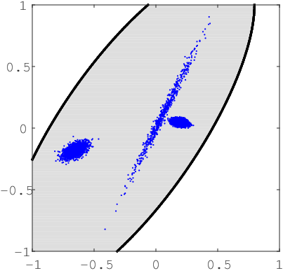
(a) $d=2$

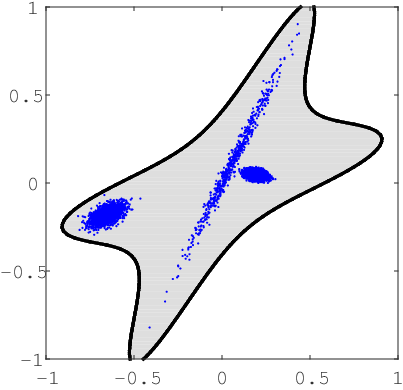
(b) $d=4$

Figure 2: Minimum-volume covering ellipsoid ($d=2$) and quartic ($d=4$) for a $10000$-point dataset.

The test cases show that the algorithm works well with data in two or three dimensions. Figure 2 shows the minimum-volume covering ellipsoids and quartic for a $10000$-point dataset on the plane. This figure also indicates that when the degree $d$ of the polynomial $\theta$ increases, the corresponding level set provides tighter approximation of the dataset. When $n=3$, we have run the algorithm for datasets with up to $100,000$ points. The number of iterations we need is about $6$ and it decreases when we decrease the number of points to be covered. We also have results for datasets with $10,000$ points when $n=10$. However, the time to prepare moment matrices increases significantly in terms of the dimension. We need to prepare $O(n^{2})$ square matrices of size $O(n^{2})$ as data input for the relaxation if $r=2$. If the probability measure is supported on $m$ points, then the total computational time to prepare all necessary moment matrices is proportional to $O(n^{7}m)$. Clearly, this algorithm is more suitable for datasets in low dimensions with a large number of points. The computational time could be reduced significantly if we implement additional heuristic to find a good initial subset instead of the whole set. A problem-specific SDP code that exploits the data structure of the relaxation could be useful for datasets in higher dimensions.

4.3 Separation Problem via Ellipsoids

4.3.1 Problem Formulation

The separation problem via ellipsoids with two datasets $S_{1}\subset\mathbb{R}^{n}$ and $S_{2}\subset\mathbb{R}^{n}$ is to find an ellipsoid that contains one set, for example, $S_{1}$, but not the other, which is $S_{2}$ in this case. If we represent the ellipsoid as the set $\Omega:=\left\{\boldsymbol{x}\in\mathbb{R}^{n}:-\boldsymbol{x}^{\prime}\boldsymbol{Q}\boldsymbol{x}+\boldsymbol{b}^{\prime}\boldsymbol{x}+c\geq 0\right\}$ with $\boldsymbol{Q}=\boldsymbol{Q}^{\prime}\succ\boldsymbol{0}$, then similar to the minimum-volume covering ellipsoid problem, we can formulate the separation problem as follows:

$${\cal P}\stackrel{{\scriptstyle\bigtriangleup}}{{=}}\left[\begin{array}[]{rl}\inf_{\boldsymbol{Q},\boldsymbol{b},c}&\log\det\boldsymbol{Q}^{-1}\\ \mathop{\rm s.t.}&-\boldsymbol{x}^{\prime}\boldsymbol{Q}\boldsymbol{x}+\boldsymbol{b}^{\prime}\boldsymbol{x}+c\geq 0,\quad\forall\boldsymbol{x}\in S_{1},\\ &-\boldsymbol{x}^{\prime}\boldsymbol{Q}\boldsymbol{x}+\boldsymbol{b}^{\prime}\boldsymbol{x}+c\leq 0,\quad\forall\boldsymbol{x}\in S_{2},\\ &\left[\begin{array}[]{cc}\boldsymbol{Q}&\frac{1}{2}\boldsymbol{b}\\ \frac{1}{2}\boldsymbol{b}^{\prime}&1-c\end{array}\right]\succeq\boldsymbol{0}.\end{array}\right]$$ (15)

4.3.2 Computational Results

Similar to the minimum-volume ellipsoid problem, the algorithm for this separation problem can be implemented with $r=2$. With YALMIP interface and SDPT3 solver, the logdet objective function is converted to geometric mean function, which is $-(\det\boldsymbol{Q})^{1/n}$. If the problem is feasible, the optimal solution will have $\boldsymbol{Q}\succ\boldsymbol{0}$, which means that the objective value is strictly negative. This can be considered as a sufficient condition to determine that the problem is feasible. In each iteration of the algorithm, if the optimal value is zero ($\boldsymbol{Q}=\boldsymbol{0}$, $\boldsymbol{b}=\boldsymbol{0}$, and $c=0$ is a feasible solution for the subproblem solved in each iteration), then we can stop and conclude that the problem is infeasible. Existence of the critical subset that determines the problem infeasibility can be proved using the same arguments as in the proof of Theorem 3 for the feasibility problem:

$${\cal P}\stackrel{{\scriptstyle\bigtriangleup}}{{=}}\left[\begin{array}[]{rl}\inf_{\boldsymbol{Q},\boldsymbol{b},c,d}&d\\ \mathop{\rm s.t.}&-\boldsymbol{x}^{\prime}\boldsymbol{Q}\boldsymbol{x}+\boldsymbol{b}^{\prime}\boldsymbol{x}+c\geq 0,\quad\forall\boldsymbol{x}\in S_{1},\\ &-\boldsymbol{x}^{\prime}\boldsymbol{Q}\boldsymbol{x}+\boldsymbol{b}^{\prime}\boldsymbol{x}+c\leq d,\quad\forall\boldsymbol{x}\in S_{2},\\ &\left[\begin{array}[]{cc}\boldsymbol{Q}&\frac{1}{2}\boldsymbol{b}\\ \frac{1}{2}\boldsymbol{b}^{\prime}&1-c\end{array}\right]\succeq\boldsymbol{0}.\end{array}\right]$$ (16)

As for the minimum-volume covering ellipsoid problem, we have implemented a variant of the minimum-volume separation ellipsoid to separate datasets by using quartic polynomials. In order to test the algorithm, we generate datasets $S_{1}$ and $S_{2}$ as for the minimum-volume covering ellipsoids problem. In most cases, if we run the algorithm for $S_{1}$ and $S_{2}$, we get infeasibility results. In order to generate separable datasets, we run the minimum-volume covering ellipsoid algorithm for $S_{1}$ and generate the separable set $S_{2}^{\prime}$ from $S_{2}$ by selecting all points that are outside the ellipsoid. We also try to include some points that are inside the ellipsoid to test the cases when $S_{1}$ and $S_{2}^{\prime}$ are separable by a different ellipsoid rather than the minimum-volume ellipsoid that covers $S_{1}$.

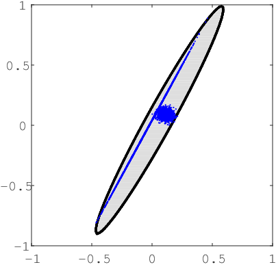
(a) Minimum-volume covering ellipsoid

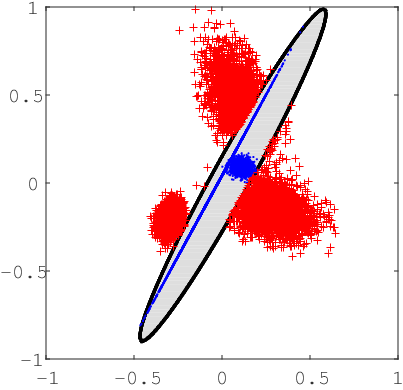
(b) Separating ellipsoid

Figure 3: Separating ellipsoid is the same as the minimum-volume covering ellipsoid.

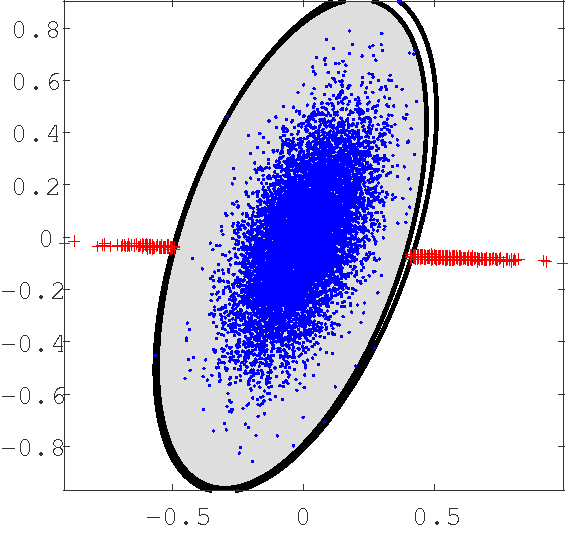
Figure 4: Separating ellipsoid is different from the minimum-volume covering ellipsoid.

(a) Separable datasets $S_{1}$ and $S_{2}$

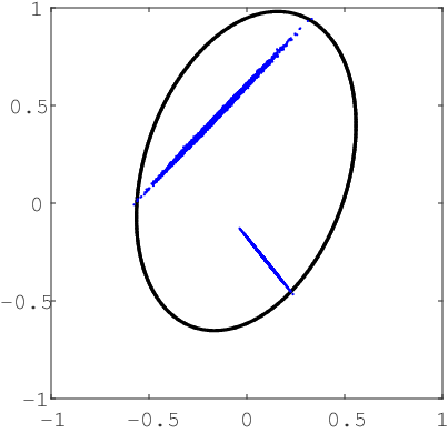
(b) Minimum-volume ellipsoid for $S_{1}$

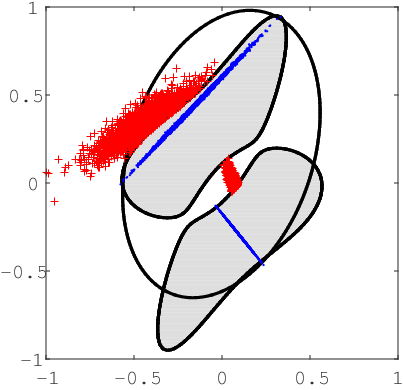
(c) Separating quartic for $S_{1}$ and $S_{2}$

Figure 5: Separating quartic for two $10000$-point datasets.

The test cases show that the algorithm can detect problem infeasibility and in the separable case, finds an ellipsoid that separates two datasets. Figure 3 shows the separation of two datasets on the plane with $10000$ points by the minimum-volume ellipsoid, while Figure 4 represents the case when a different ellipsoid is needed to separate two particular sets. We also ran the algorithm for datasets with $n=3$ and $n=10$. Similar remarks can be made with respect to data preparation and other algorithmic issues as in Section 4.2.2. In general, the algorithm is suitable for datasets in low dimensions with a large number of points.

Figure 5 shows an example where there is no ellipsoid that can separate two given datasets $S_{1}$ and $S_{2}$. We indicate the border of the minimum-volume covering ellipsoid for the dataset $S_{1}$ as well as the level set of the separating quartic for $S_{1}$ and $S_{2}$. In such cases, one has to rely on higher degree polynomials to be able to separate the two datasets.

References

• [1] E. D. Andersen and K. D. Andersen. The Mosek Interior Point Optimizer for Linear Programming: An Implementation of the Homogeneous Algorithm. In Hans Frenk, Kees Roos, Tamás Terlaky, and Shuzhong Zhang, editors, High Performance Optimization, volume 33 of Applied Optimization, pages 197–232. Springer US, 2000.
• [2] E. R. Barnes. An algorithm for separating patterns by ellipsoids. IBM Journal of Research and Development, 26(6):759–764, 1982.
• [3] A. Ben-Tal, E.E. Rosinger, and A. Ben-Israel. A Helly-type theorem and semi-infinite programming. In C.V. Coffman and G.J. Fix, editors, Constructive Approaches to Mathematical Models, pages 127–135. Academic Press, New York, 1979.
• [4] G. Calafiore. Approximation of n-dimensional data using spherical and ellipsoidal primitives. IEEE Transactions on Systems, Man, and Cybernetics, Part A, 32(2):269–278, 2002.
• [5] R. E. Curto and L. A. Fialkow. The truncated complex K-moment problem. Transactions of the American Mathematical Society, 352(6):2825–2855, 2000.
• [6] F. Glineur. Pattern separation via ellipsoids and conic programming. In Mémoire de DEA. Faculté Polytechnique de Mons, Belgium, September 1998.
• [7] LLC Gurobi Optimization. Gurobi Optimizer Reference Manual, 2018.
• [8] D. Henrion and J. B. Lasserre. Solving nonconvex optimization problems. IEEE Control System Magazine, 24:72–83, 2004.
• [9] F. John. Extreme problems with inequalities as subsidiary conditions. In Studies and Essays Presented to R. Courant on his 60th Birthday, pages 187–204. Wiley Interscience, New York, 1948.
• [10] J. B. Lasserre. Global optimization with polynomials and the problem of moments. SIAM Journal on Optimization, 11(3):796–817, 2001.
• [11] Jean B. Lasserre. A New Look at Nonnegativity on Closed Sets and Polynomial Optimization. SIAM J. Opt, 21(3):864–885, 2011.
• [12] M. Laurent. Revisiting two theorems of Curto and Fialkow on moment matrices. Proceedings of the American Mathematical Society, 133(10):2965–2976, 2005.
• [13] J. Löfberg. YALMIP : A Toolbox for Modeling and Optimization in MATLAB. In Proceedings of the CACSD Conference, Taipei, Taiwan, 2004.
• [14] A. Magnani, S. Lall, and S. Boyd. Tractable fitting with convex polynomials via sum-of-squares. In Proceedings of the 44th IEEE Conference on Decision and Control, Seville, Spain, December 2005.
• [15] J. B. Rosen. Pattern separation by convex programming. Journal of Mathematical Analysis and Applications, 10:123–134, 1965.
• [16] Jos F. Sturm. Using SeDuMi 1.02, a MATLAB toolbox for optimization over symmetric cones, 1998.
• [17] P. Sun and R. M. Freund. Computation of Minimum-Volume Covering Ellipsoids. Operations Research, 52(5):690–706, 2004.
• [18] Michael J. Todd and E. Alper Yildirim. On Khachiyan’s algorithm for the computation of minimum-volume enclosing ellipsoids. Discrete Applied Mathematics, 155(13):1731 – 1744, 2007.
• [19] M.J. Todd. Minimum-Volume Ellipsoids: Theory and Algorithms. MOS-SIAM Series on Optimization. SIAM, 2016.
• [20] R. H. Tütüncü, K. C. Toh, and M. J. Todd. Solving semidefinite-quadratic-linear programs using SDPT3. Mathematical Programming, 95(2):189–217, 2003.
• [21] Lieven Vandenberghe, Stephen Boyd, and Shao-Po Wu. Determinant Maximization with Linear Matrix Inequality Constraints. SIAM Journal on Matrix Analysis and Applications, 19(2):499–533, 1998.