Production of pairs via
subprocess
with photon transverse momenta
Abstract
We discuss production of pairs in proton-proton collisions induced by two-photon fusion including, for a first time, transverse momenta of incoming photons. The unintegrated inelastic fluxes (related to proton dissociation) of photons are calculated based on modern parametrizations of deep inelastic structure functions in a broad range of their arguments ( and ). In our approach we can get separate contributions of different helicities states. Several one- and two-dimensional differential distributions are shown and discussed. The present results are compared to the results of previous calculations within collinear factorization approach. Similar results are found except of some observables such as e.g. transverse momentum of the pair of and . We find large contributions to the cross section from the region of large photon virtualities. We show decomposition of the total cross section as well as invariant mass distribution into the polarisation states of both W bosons. The role of the longitudinal structure function is quantified. Its inclusion leads to a 4-5 % decrease of the cross section, almost independent of .
I Introduction
Recently the partonic processes initiated by one or two photons in hadronic collisions at the Large Hadron Collider (LHC) are becoming an active field of research. The corresponding theoretical approach requires the calculation of photon fluxes in the proton-proton collision. The majority of practical approaches focused on a collinear factorization approach where the momentum of the colliding photon is collinear to the parent proton momentum. For a comprehensive review on photon-photon fusion reactions, see Budnev:1974de . Recently, for the conditions of LHC, photon-photon fusion was discussed in the context of lepton pairs daSilveira:2014jla ; Luszczak:2015aoa , LSR2015 or possible signals beyond the Standard Model, such as the production of charged Higgs bosons LS2015 . In Ref.LSR2015 it was shown that photon-photon partonic processes are important for large invariant masses of pairs.
Several groups that provide the high-energy community with parton distribution functions included photons as partons in the proton Martin:2004dh ; Ball:2013hta ; Schmidt:2015zda ; Giuli:2017oii , solving the corresponding coupled DGLAP evolution equations.
This strategy differs from the one adopted in Ref. daSilveira:2014jla ; Luszczak:2015aoa (see also Ref.Ginzburg:1998vb ), where following Ref. Budnev:1974de , the photon fluxes had been calculated in a data-driven way using their relation to the well-measured proton structure functions. Subsequently, such a data-driven approach was taken up in Refs. Manohar:2016nzj ; Manohar:2017eqh .
The transverse momenta of photons were included so far only for or subprocesses daSilveira:2014jla ; Luszczak:2015aoa . There we identified corners of phase space where transverse momenta of photons (or their virtualities) are large.
In the present paper we extend our studies to the production of pairs. We expect that here the virtualities of photons may be much larger than for production.
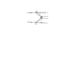
Particularly interesting is the region of large invariant masses of the system where the diphoton mechanism becomes one of the most important contributions for pair production. We shall compare the calculation within the -factorization approach with those obtained previously in the collinear approximation. We shall discuss all types of processes as shown in Fig.1.
The subprocess is interesting also in the context of searches of effects beyond Standard Model effects Chapon:2009hh ; Pierzchala:2008xc , such as anomalous quartic gauge-boson couplings. First experimental studies on anomalous couplings were already presented recently both by the CMS and ATLAS collaborations Khachatryan:2016mud ; Aaboud:2016dkv . We expect that our present estimate within the Standard Model will be therefore a useful reference point in searches beyond Standard Model. We shall also present a separate contribution for longitudinal boson which is interesting in the contex of final state interactions and/or searches for possible resonances, see for example Kilian:2015opv ; Delgado:2016rtd ; Szleper:2014xxa .


II Accounting for transverse momenta of photons
In this section we will include the transverse momentum of photons, so that the distributions of the transverse momentum of the pair and the azimuthal angle between the ’s have a nontrivial behaviour already at the lowest order. In daSilveira:2014jla ; Luszczak:2015aoa a -factorization approach for the -fusion reactions in the high-energy limit of the -collision has been given. This approach has its domain of applicability in the region of small momentum fractions carried by photons.
In this case, the unintegrated photon distributions can be calculated from the proton structure function alone in a data-driven way.
A broader range of applicability has the generalized equivalent-photon approximation of Budnev:1974de , in which a whole density matrix of photons appears. In some instances, for example when the masses squared of produced particles are much larger than the typical virtualities of photons, the density matrix simplifies and only transverse polarizations in the center-of-mass of colliding photons are important. We will adopt this approach for our numerical calculations of bosons below.
In both -dependent approaches described above, the cross section for production can be written in the form
where the indices denote elastic or inelastic final states. The longitudinal momentum fractions of photons are obtained from the rapidities and transverse momenta of final state as:
| (2) |
For photons which carry transverse polarization in the -cms frame, we write the relevant “off-shell” cross section as:
where the matrix element in terms of transverse momenta of incoming photons is given by
| (4) | |||||
with . The helicity matrix elements for the process are taken from Ref. Nachtmann:2005en , where one can also find explicit helicity states defined in the cm-frame of the pair. It is useful to decompose the matrix element further, using the identity
| (5) | |||||
Here the antisymmetric symbol is defined by , and
| (6) |
furthermore
| (7) |
We then obtain for the helicity-matrix element
| (8) | |||||
Together with these matrix elements, we use the photon fluxes from Budnev:1974de . We write the photon distribution differentially as
| (9) |
The virtuality of the photon carrying momentum fraction and transverse momentum is
| (10) |
where is the invariant mass of the proton remnant in the final state. Then using
| (11) |
we can write the fluxes from Budnev:1974de as
| (12) | |||||
and similarly for the elastic piece
These fluxes differ from the ones from Ref. daSilveira:2014jla ; Luszczak:2015aoa , which apply in the high energy limit. The difference in these approaches is threefold: firstly, fluxes in Ref. daSilveira:2014jla ; Luszczak:2015aoa also include a contribution from longitudinal polarizations of photons in the cms, secondly within the accuracy of the high-energy limit, the fluxes of daSilveira:2014jla ; Luszczak:2015aoa depend on only, and thirdly these fluxes must be accompanied by the corresponding off-shell matrix element. Notice that in (12) instead of , one may use the pair , where
| (14) |
is the longitudinal structure function of the proton.
III Collinear-factorization approach
In some cases it can be sufficient to neglect the transverse momenta of partons. Then photons are treated as collinear partons in a proton. Like other parton densities, the photon distribution is a function of the longitudinal momentum fraction carried by the photon and the factorization scale of the hard process the photon participates in.
A number of parametrizations of the photon parton distributions have become available recently Martin:2004dh ; Ball:2013hta ; Schmidt:2015zda ; Giuli:2017oii ; Manohar:2016nzj ; Manohar:2017eqh . Most of them are based on including photons into the coupled DGLAP evolution equations for quarks and gluons Martin:2004dh ; Ball:2013hta ; Schmidt:2015zda ; Giuli:2017oii and attempt to extract the photon distributions from either global fits or fits to processes that are deemed to have a strong sensitivity to the photon distribution. A different approach is taken in Ref.Manohar:2016nzj ; Manohar:2017eqh , where similarly to Ref.Luszczak:2015aoa a data driven approach is taken. An explicit coherent contribution is related to the electromagnetic form factors of a proton. A second contribution is related to the proton structure functions and .
In the collinear approach the photon-photon contribution to inclusive cross section for production can be written as:
| (15) |
Here
| (16) |
Above indices and denote , i.e. they correspond to elastic or inelastic components similarly as for the -factorization discussed in section II above. The factorization scale is chosen as .
Calculations with collinear partons from eq. 15 have the drawback, that at the lowest order the produced two-body system is strictly in back-to-back kinematics. Consequently the distribution in transverse momentum of the produced pair is a delta-function. Similarly behaved the distribution of the azimuthal angle between the produced particles, which is a delta function centered at .
It should be made clear, however, that in Monte-Carlo simulations of the inclusive -pair production, collinear cross sections, such as the one given by (15) can be embedded into events including e.g. initial state emissions from parton showers, which will give a finite transverse momentum to the -pair. The effect of highly virtual photons must then be accounted for by matching to higher order processes such as e.g. or . The necessary rather sophisticated computational techniques are described e.g. in Alwall:2014hca . We are not aware of calculations of the processes of interest here in this approach and prefer to stick to the more straightforward -factorization described in the previous section. Also, it should be noted that when we refer to the collinear approximation in the remainder of the text, we always refer to calculations from Eq.(15).
IV Results
In this section we shall show our results for the -factorization approach. We shall concentrate first on the inelastic-inelastic contribution (see Fig.1). In the present paper we will not include experimental cuts but rather consider full phase space calculations.
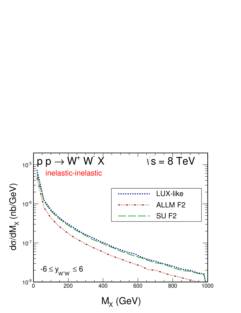
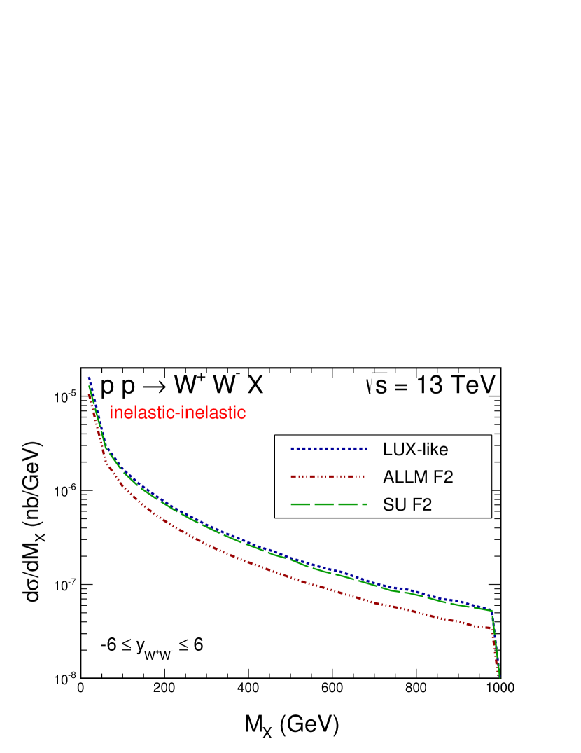
We start from showing the cross sections using different parametrizations of proton structure functions.
Here we use the following options:
-
1.
the Abramowicz-Levy-Levin-Maor fit Abramowicz:1991xz ; Abramowicz:1997ms used previously also in Luszczak:2015aoa , abbreviated here ALLM.
-
2.
a newly constructed parametrization, which at uses an NNLO calculation of and from NNLO MSTW 2008 partons Martin:2009iq . It employs a useful code by the MSTW group Martin:2009iq to calculate structure functions. At this fit uses the parametrization of Bosted and Christy Bosted:2007xd in the resonance region, and a version of the ALLM fit published by the HERMES Collaboration Airapetian:2011nu for the continuum region. It also uses information on the longitudinal structure function from SLAC Abe:1998ym . As the fit is constructed closely following the LUXqed work Ref.Manohar:2017eqh , we call this fit LUX-like.
-
3.
a Vector-Meson-Dominance model inspired fit of proposed in SU at low , which is completed by the same NNLO MSTW structure function as above at large . This fit is labelled SU for brevity.
One can see from Table 1 that the largest inelastic-inelastic component is in all calculations systematically bigger than the elastic-elastic component, which gives the smallest contribution. For the case of production of or via fusion all components were of the same size Luszczak:2015aoa .
| contribution | 8 TeV | 13 TeV |
|---|---|---|
| LUX-like | ||
| 0.214 | 0.409 | |
| 0.214 | 0.409 | |
| 0.478 | 1.090 | |
| ALLM97 F2 | ||
| 0.197 | 0.318 | |
| 0.197 | 0.318 | |
| 0.289 | 0.701 | |
| SU F2 | ||
| 0.192 | 0.420 | |
| 0.192 | 0.420 | |
| 0.396 | 0.927 | |
| LUXqed collinear | ||
| 0.366 | 0.778 | |
| MRST04 QED collinear | ||
| 0.171 | 0.341 | |
| 0.171 | 0.341 | |
| 0.548 | 0.980 | |
| Elastic- Elastic | ||
| (Budnev) | 0.130 | 0.273 |
| (DZ) | 0.124 | 0.267 |
We obtain cross sections of about 0.8–1 pb at = 8 TeV and 1.5–1.8 pb at = 13 TeV. This may be compared to 41.1 15.3 (stat) 5.8 (syst) 4.5 (lumi) pb (CMS CMS_inclusive ) and 54.4 4.0 (stat) 3.9 (syst) 2.0 (lumi) pb (ATLAS ATLAS_inclusive ) measured (and extrapolated) at the LHC for = 7 TeV. This shows that the two-photon production constitutes about 2 % of the total cross section. However, its relative contribution, as will be discussed below, increases with .
IV.1 One-dimensional distributions
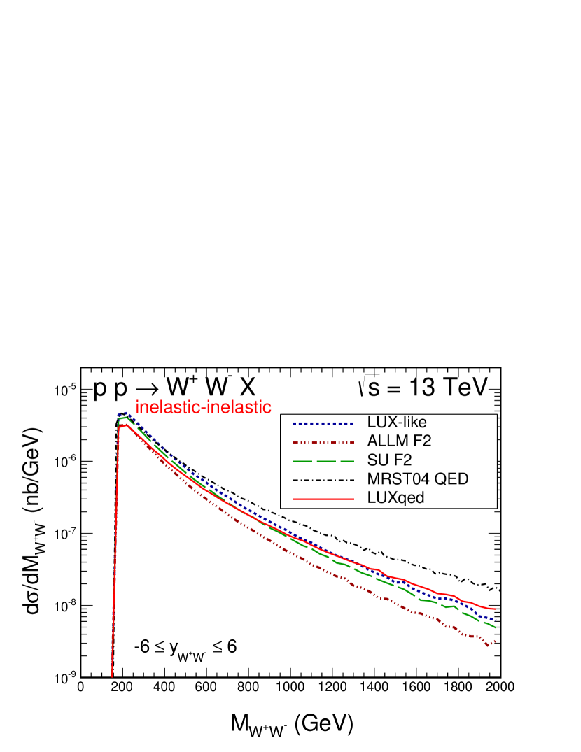
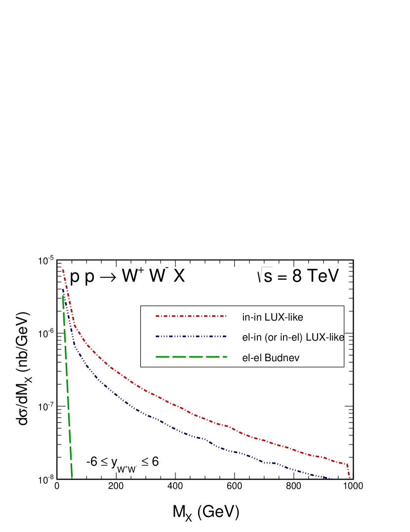
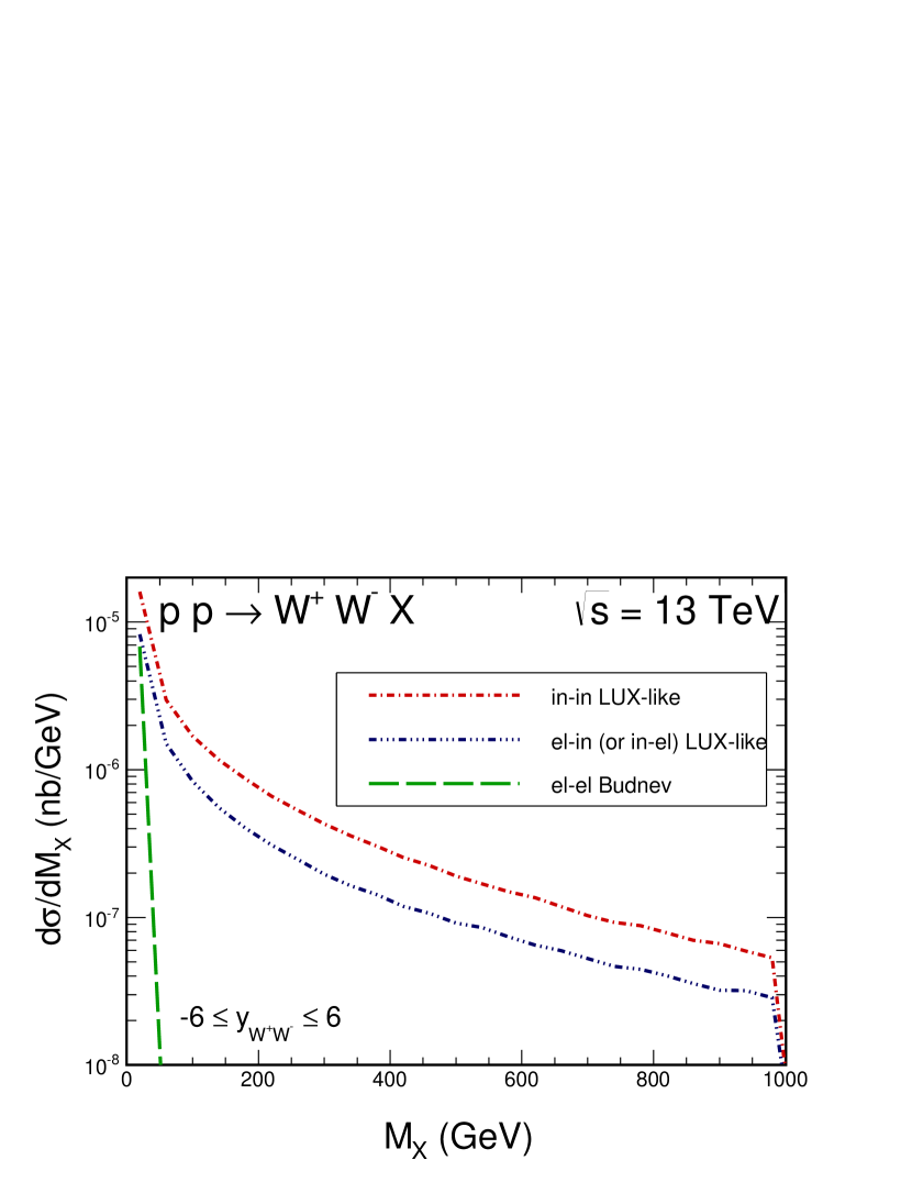
In Fig.2 we show invariant mass distributions for = 8 TeV (left panel) and = 13 TeV (right panel). The calculations have been performed with different parametrizations of structure functions including the LUX-like one. There are large uncertainties in the region of large invariant masses. The uncertainties become smaller for larger . We will compare to Ref.LSR2015 , i.e. to result of collinear calculations with the rather old MRST04 QED set Martin:2004dh (dash-dotted line). The new results should be regarded as an update of the older results in LSR2015 .

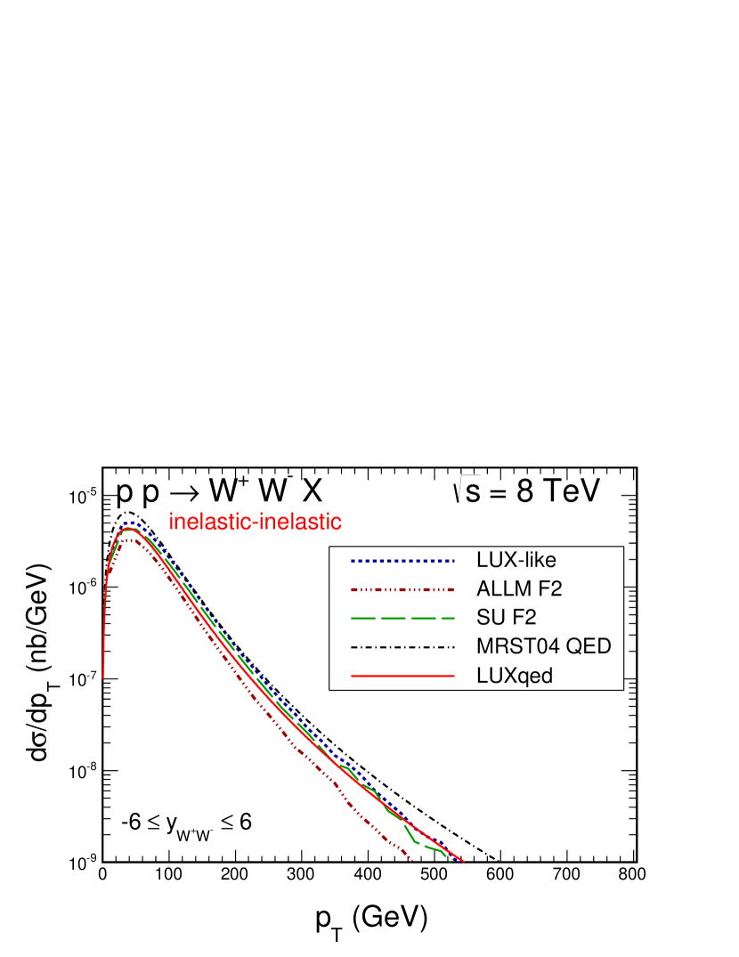
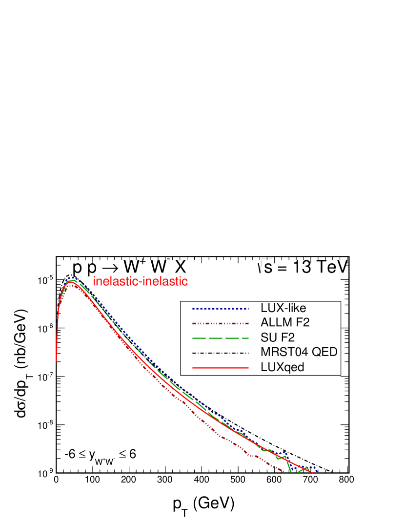
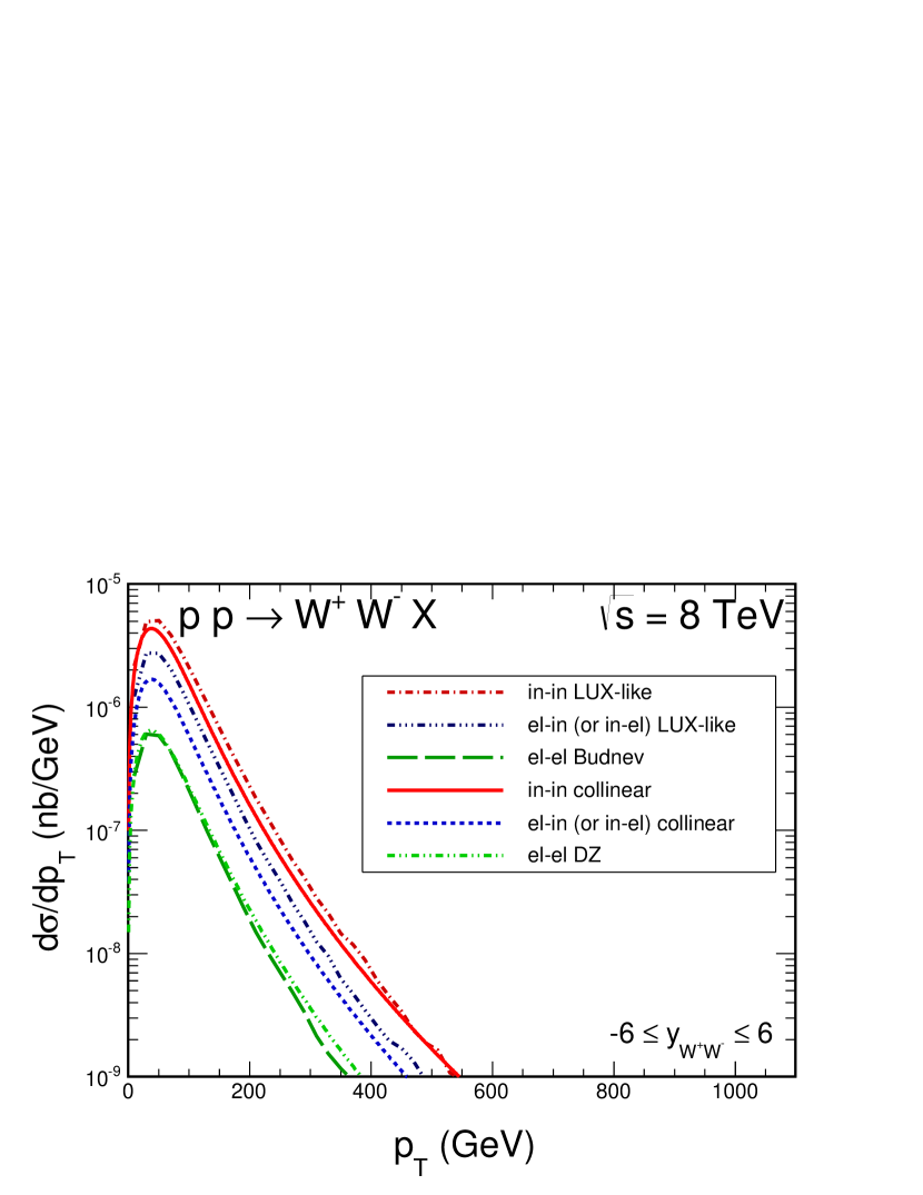
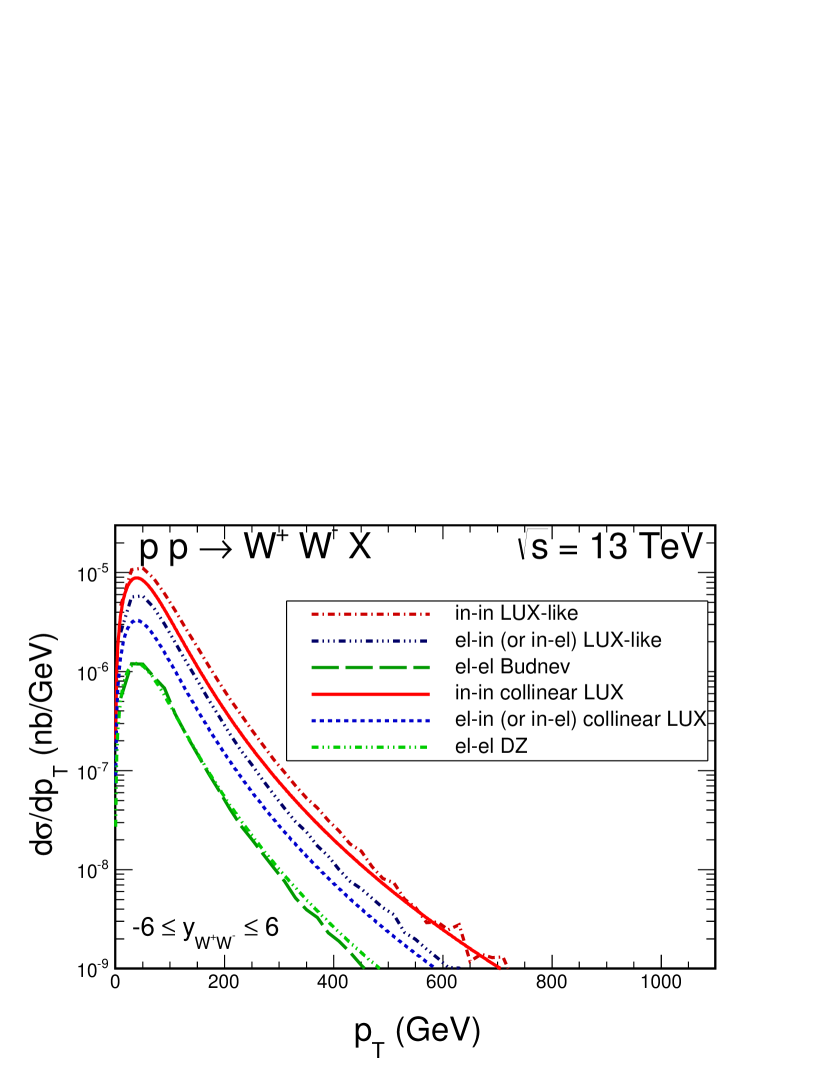
The distribution in transverse momentum of a boson is shown in Fig.3. At low transverse momenta there is a relatively small theoretical uncertainty. The result obtained with our LUX-like structure function should be considered as our best estimate.
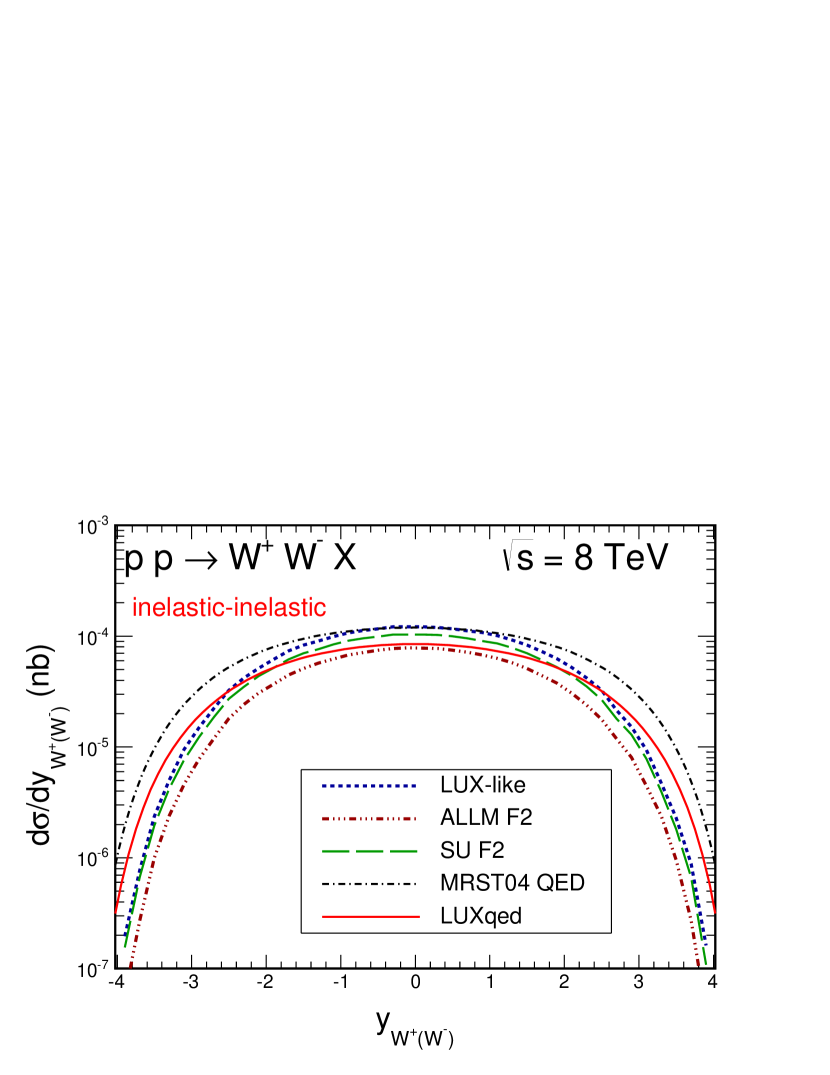
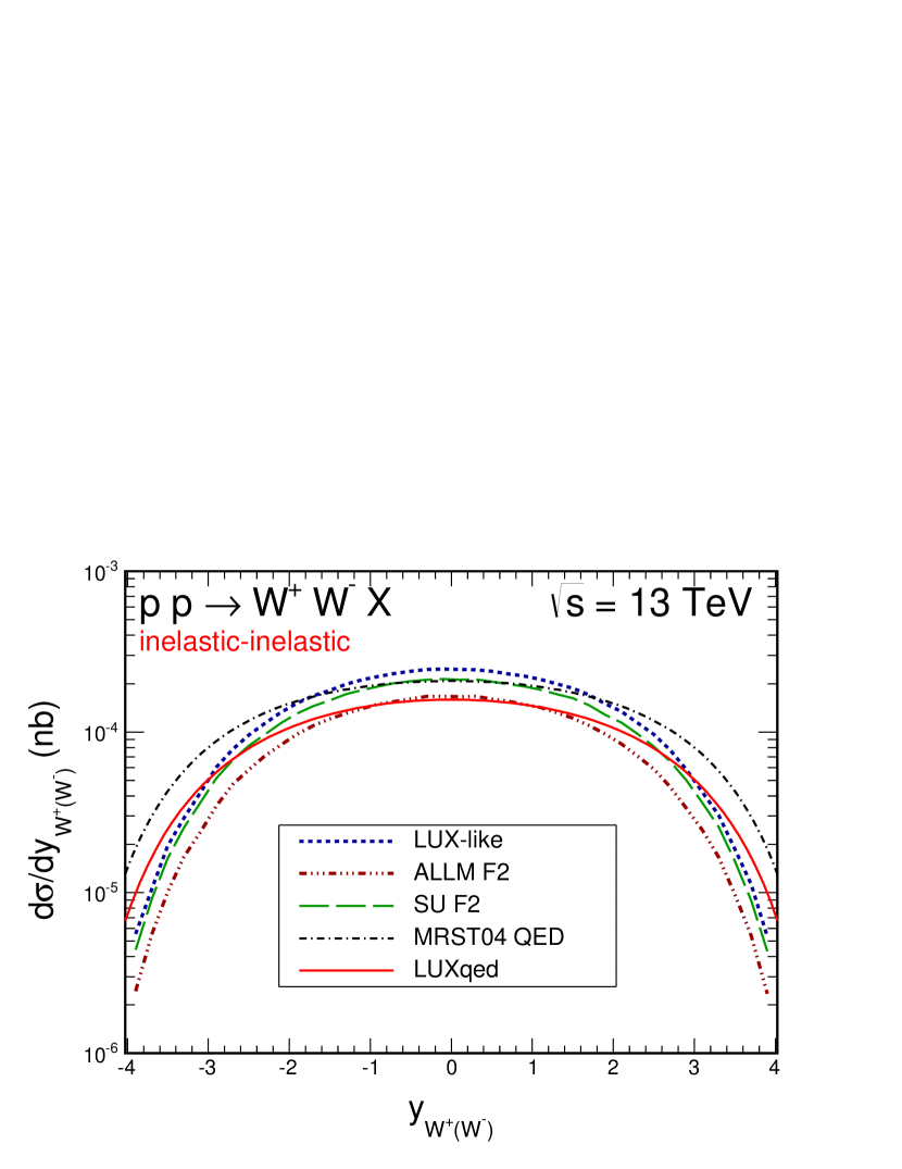
For completeness we show also rapidity distributions of bosons in Fig.4. The distribution in collinear approach extends to much larger rapidities, especially for = 13 TeV.
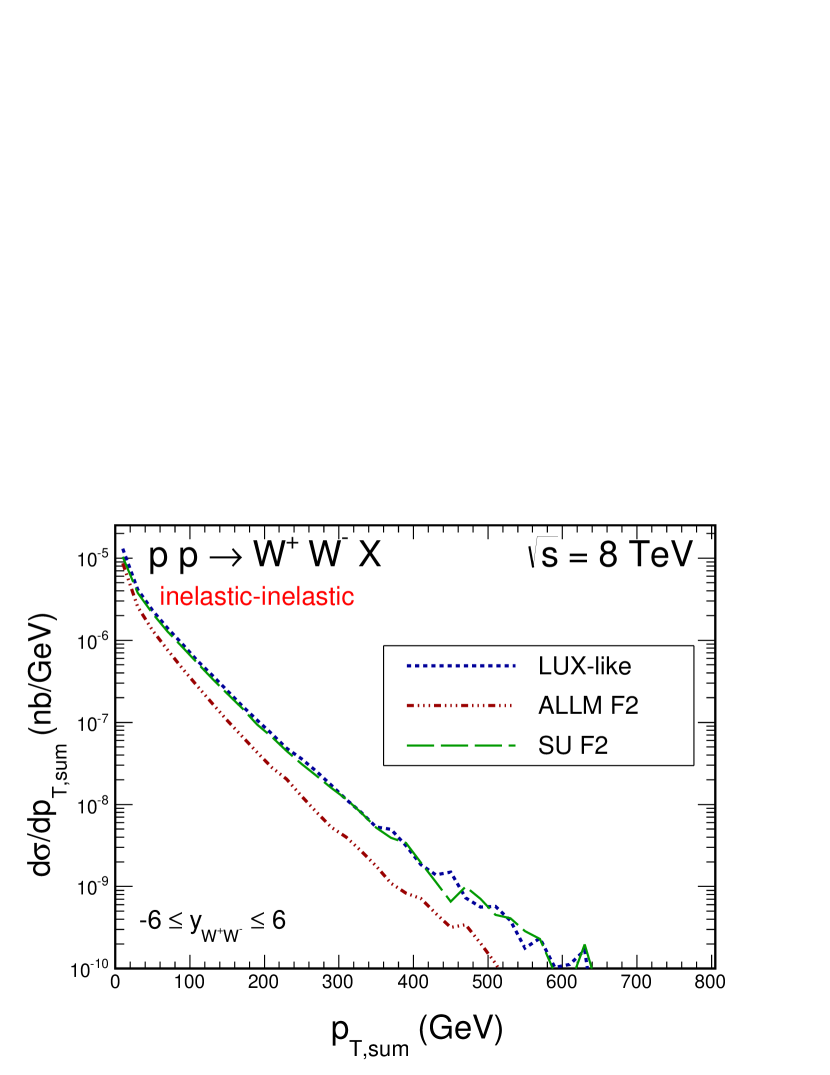
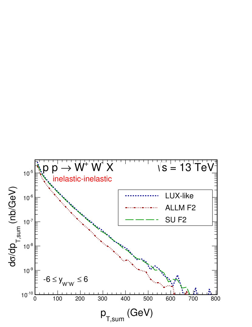
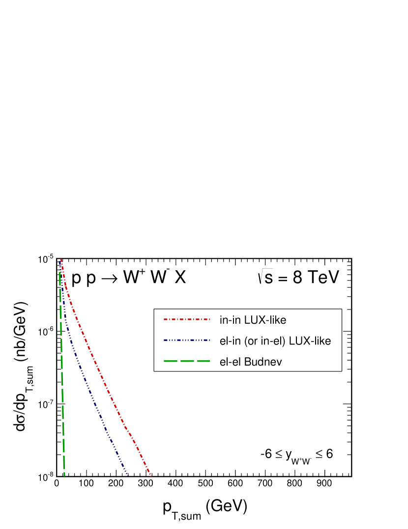
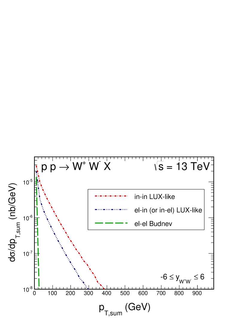
In Fig.5 we show distribution in transverse momentum of the pair, . Quite large pair transverse momenta are possible. In contrast in leading-order using collinear partons, the corresponding distribution is just a Dirac delta function at = 0. The -factorization approach should be therefore here a much better approach. This distribution is, however, a bit academic as in practice one measures only charged leptons and the neutrinos escape experimental observation, but the figure demonstrates theoretical preference of the -factorization approach over the collinear approach. The nonvanishing pair transverse momentum can influence the transverse momentum distributions of associated leptons (usually or ) when it is large. This effect will be discussed elsewhere.
Our approach also goes beyond Manohar:2016nzj ; Manohar:2017eqh in that it allows us to obtain the distribution of the mass of the proton remnant(s). These distributions are shown in Fig.6. Quite large masses of the remnant system are generated. Notice, that the larger is the invariant mass, the smaller is the rapidity gap from the proton remnant to the system. Detailed studies of this effect require a hadronisation of the remnant system, which goes beyond the scope of the present paper.
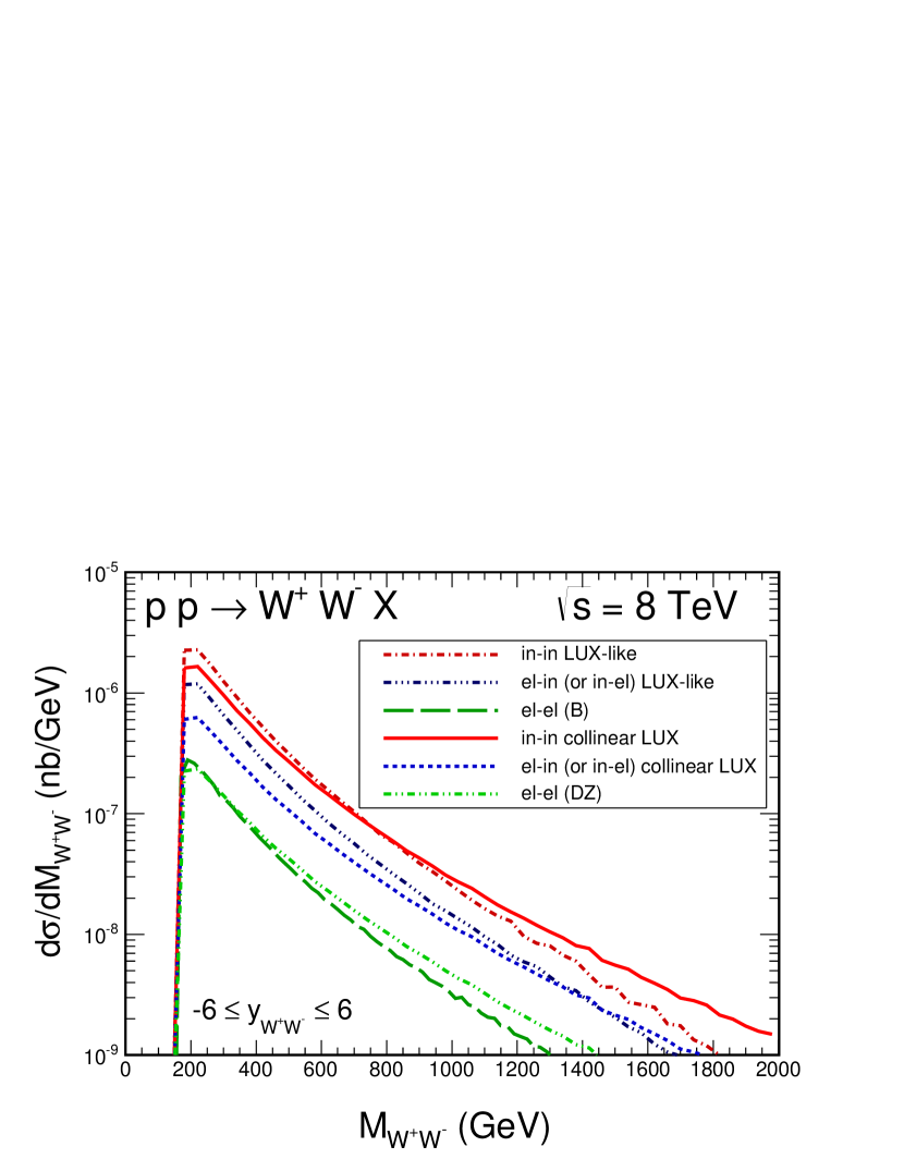
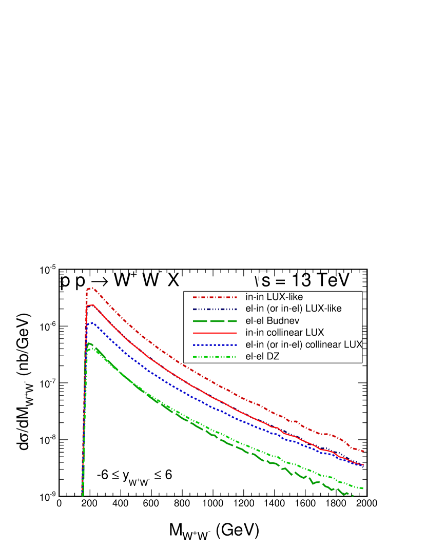
Now we shall compare results corresponding to different diagrams shown in Fig.1. We start by showing distributions in invariant mass (see Fig.7). The inelastic contributions (inelastic-inelastic, inelastic-elastic or elastic-inelastic) are larger than the purely elastic (elastic-elastic) contribution. For reference we show distributions in the collinear approach with the LUXqed structure function parametrization.
In Fig.8 we compare transverse momentum distributions for all components of Fig.1. Similar slopes are obtained for different components, while the corresponding cross sections are different.
A similar result for the pair transverse momentum distribution is shown in Fig.8. The distribution for the inelastic-inelastic contribution is broader than that for elastic-inelastic or inelastic-elastic component. The elastic-elastic contribution gives very narrow distribution compared to the two other components.
The missing mass distributions for different components are shown in Fig.10. The shape for the elastic-inelastic and inelastic-elastic is the same as that for inelastic-inelastic component. The one for the elastic-elastic contribution is just the Dirac delta function at . We shall return to the issue whether the distributions in and for the inelastic-inelastic component are correlated when discussing two-dimensional distributions of correlation character.
IV.2 Correlation observables
Now we shall proceed to two-dimensional distributions of correlation character.
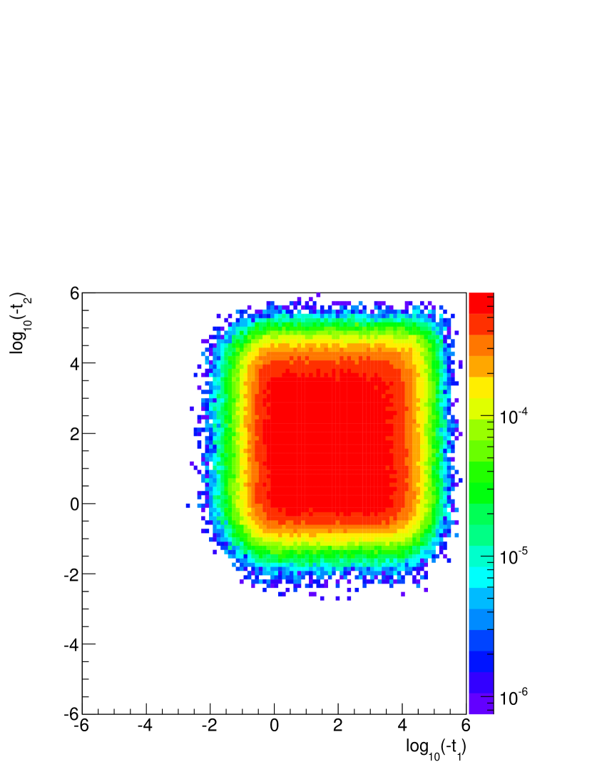
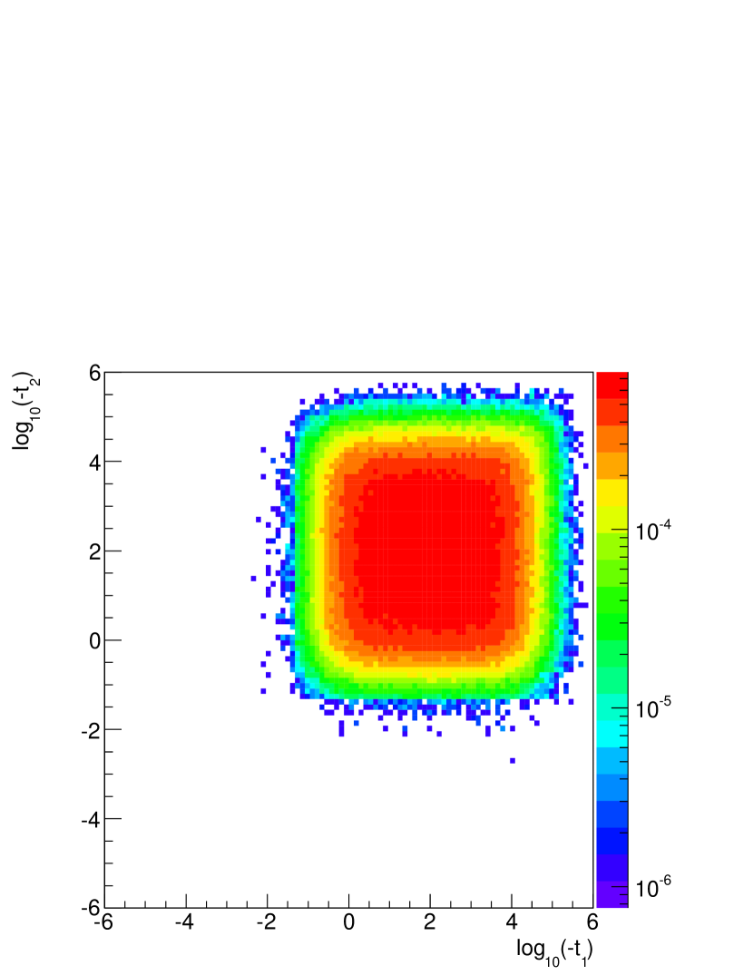
In the collinear approximation, the incoming photons are taken to be on-mass shell, i.e. massless. How the situation changes in our approach will be discussed in the following. In Fig.11 we show distribution in (please note logarithmic scales on both axes). A plateau extending to 104 GeV can be seen. The result shows that collinear-factorization approach could be far from being realistic for the production, at least in some parts of the phase space.

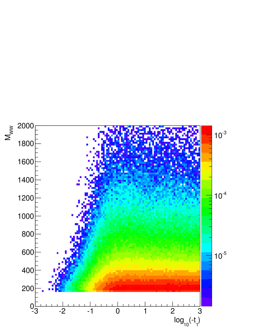
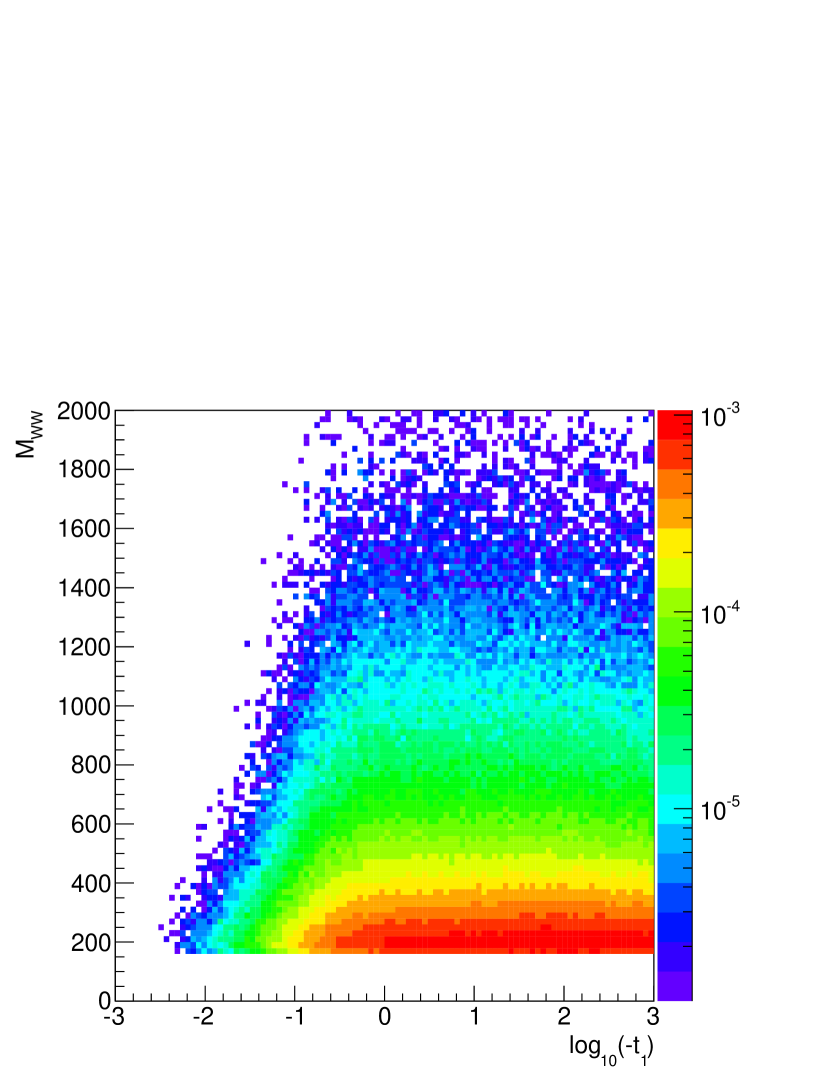
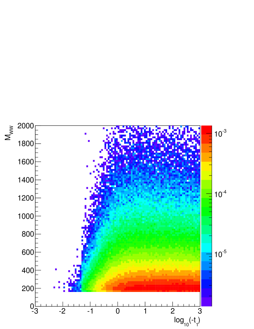
In Fig.12 we discuss correlation between or and invariant mass of the system produced in the photon-photon fusion (please note logarithmic scale in rapidity). At large there are no small virtualities of photons. Therefore the collinear-factorization approach may be expected to be better close to the threshold and worse for large invariant masses. This may be important in establishing a reference Standard Model result in the studies searching for effects beyond Standard Model. The result does not depend on the parametrization of the structure function.
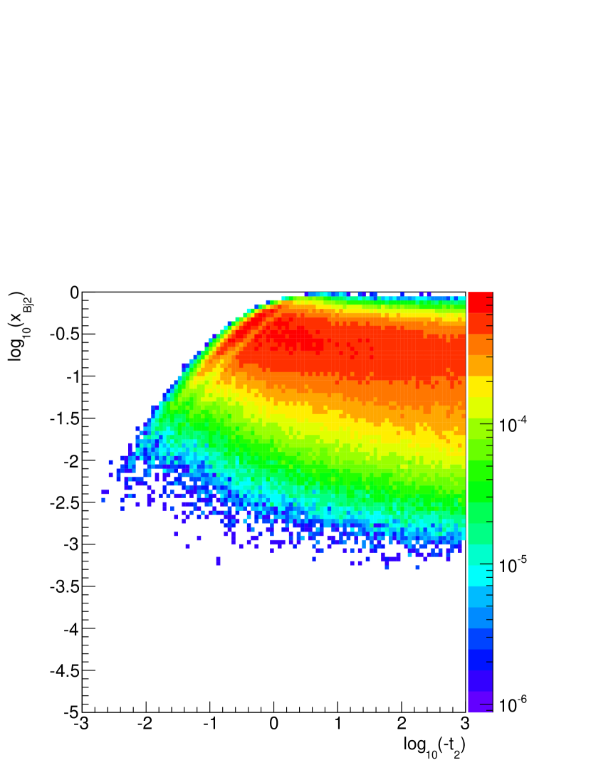
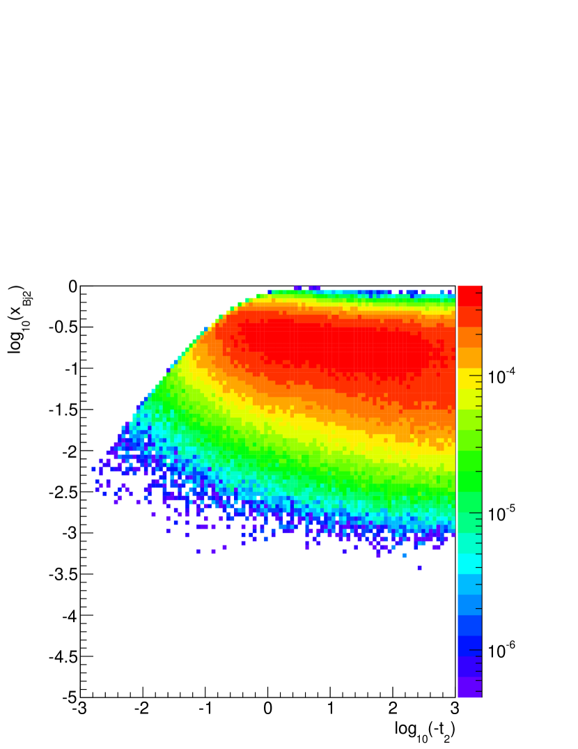
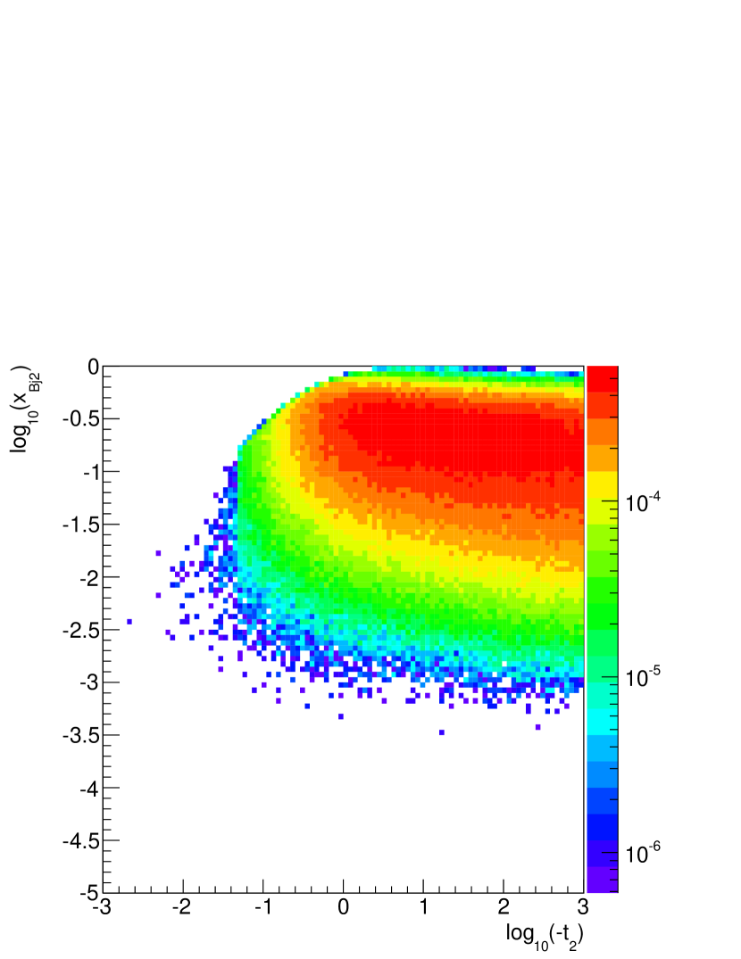
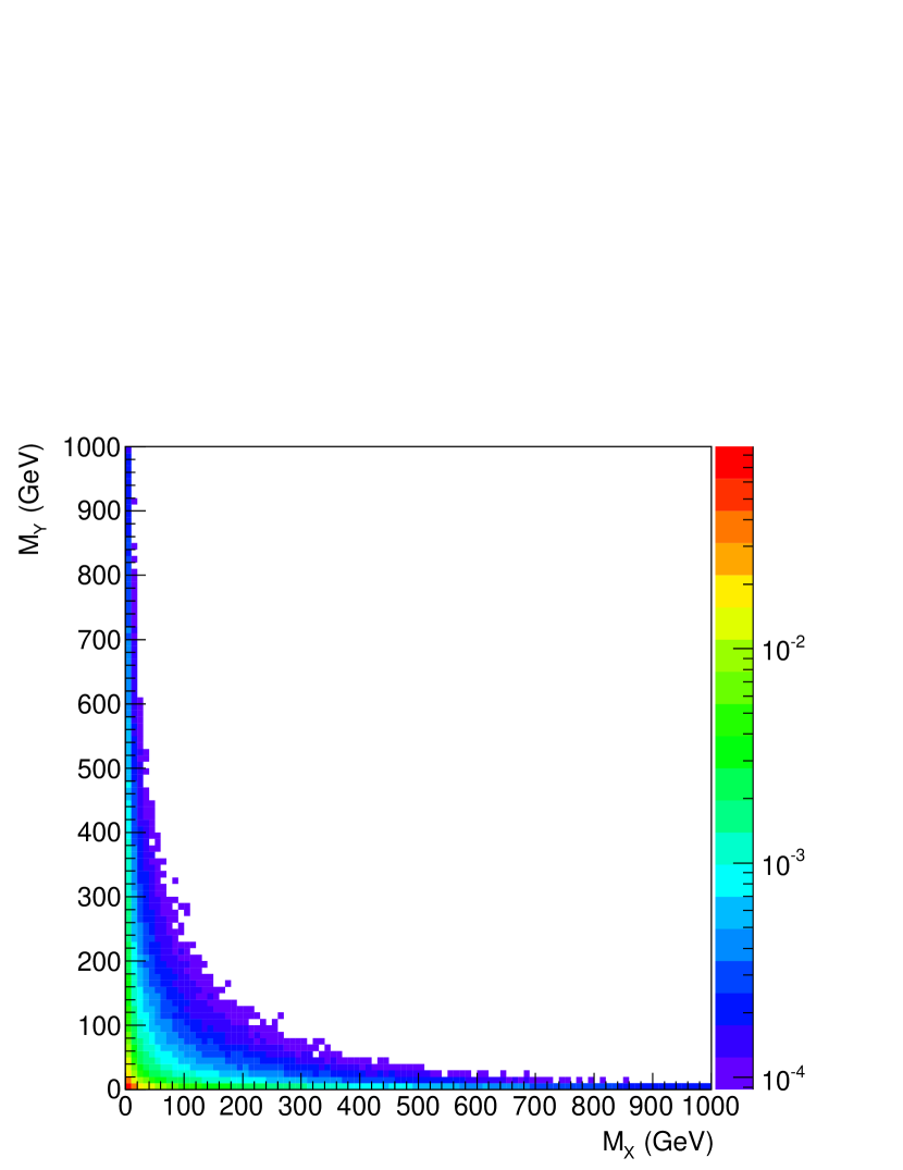
In the inelastic-inelastic case both protons undergo dissociation into a complicated final state. What happens to the remnant systems will be discussed elsewhere. Here we show whether the photon virtualities and Bjorken- values (arguments of the structure functions) are correlated. Only a small correlation can be observed. The figure shows that rather large Bjorken- give the dominant contribution. This is region corresponding to fixed-target experiments performed in 80ies and 90ies.
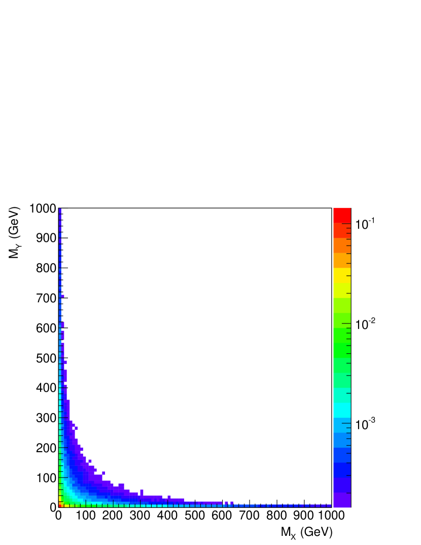
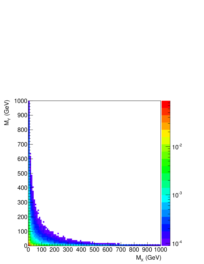
For completeness in Fig.14 we show potential correlations in masses of both dissociated systems. The maximum of the two-dimensional distribution occurs when are rather small. When one of the masses is large the second is typically small. So we typically expect situations with small rapidity gap on one side and large gap on the other side of the “centrally” produced system. This will be discussed in detail elsewhere.
IV.3 Decomposition into polarization components
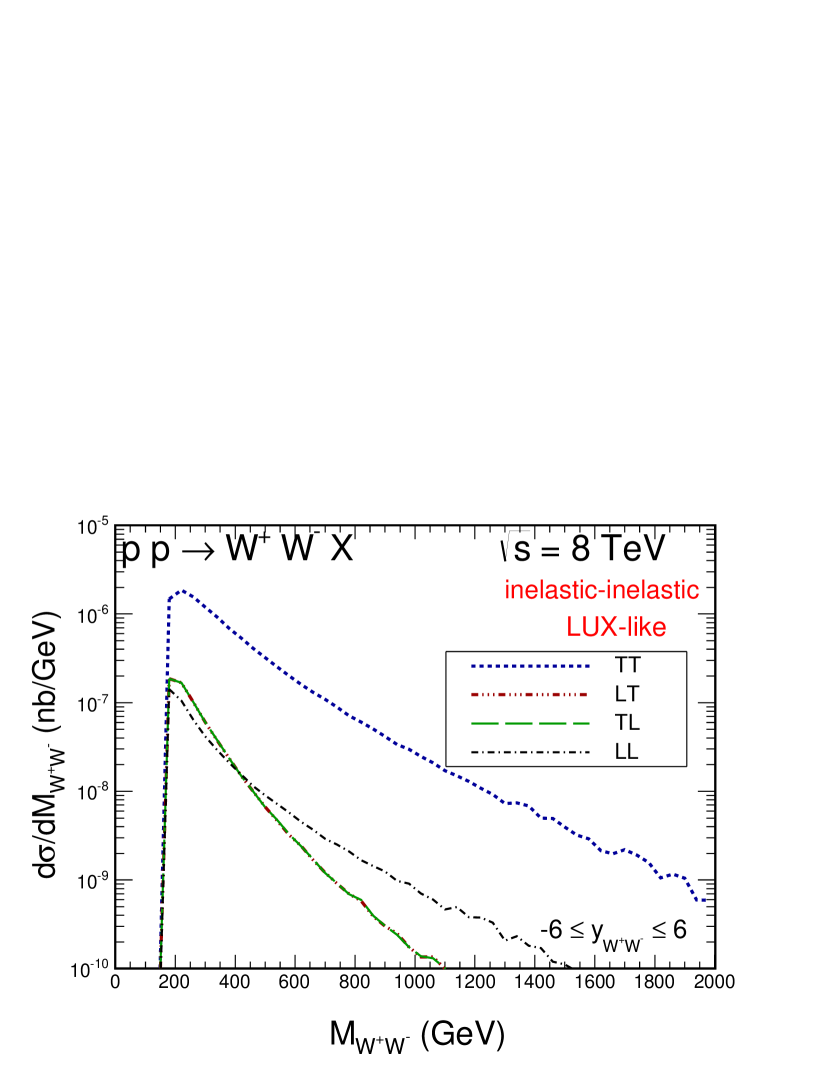
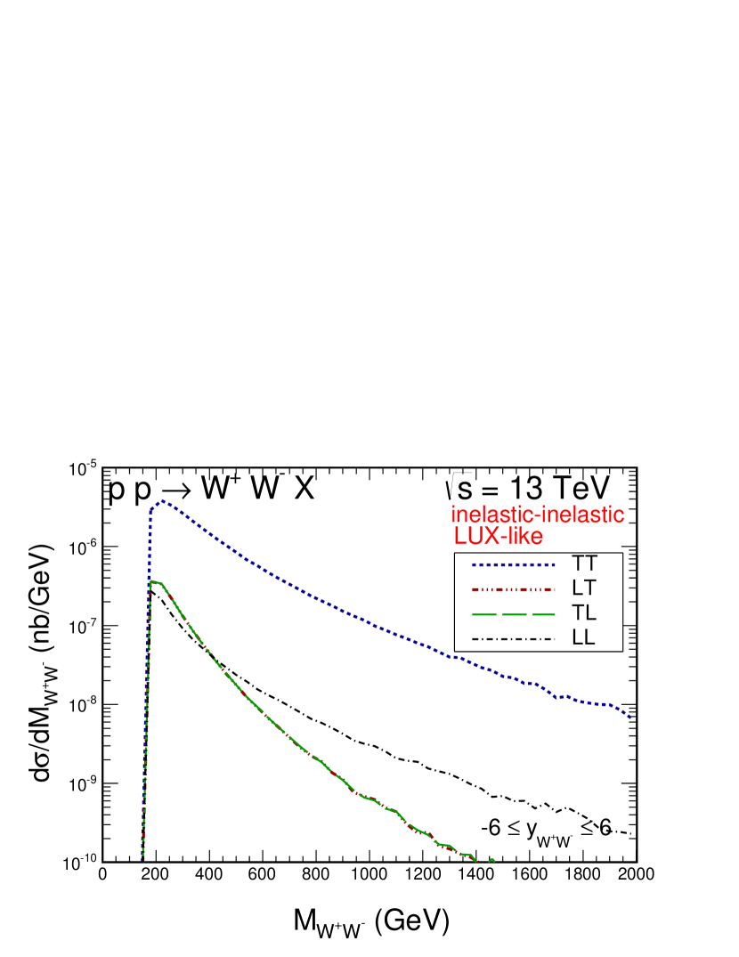
The matrix elements in Eq.(8) allow to calculate cross sections for different states of polarization of bosons (polarizations here are defined in the center-of-mass frame, for explicit formulas, see Nachtmann:2005en ). It can be seen that the TT (both ’s are transversely polarized) component is larger than 80 %. The LL (both ’s longitudinally polarized) component plays a special role in studies of interactions. However in the photon-photon fusion the cross section for production of this component is smaller than 5 % of the total cross section.
To make a thorough study of possible effects beyond the SM in the LL channel, one should include decays of ’s. Then, the small LL component can be enhanced by interference with transverse ’s.
| contribution | 8 TeV | 13 TeV |
|---|---|---|
| TT | 0.405 | 0.950 |
| LL | 0.017 | 0.046 |
| LT + TL | 0.028 + 0.028 | 0.052 + 0.052 |
| SUM | 0.478 | 1.090 |
In fact it is more interesting what happens at large invariant masses 1 TeV where effect beyond Standard Model could show up. In Fig.15 we show the decomposition into different polarization states of W bosons as a function of the invariant mass. We observe that the component dominates in the whole invariant mass region.
IV.4 Role of longitudinal structure function
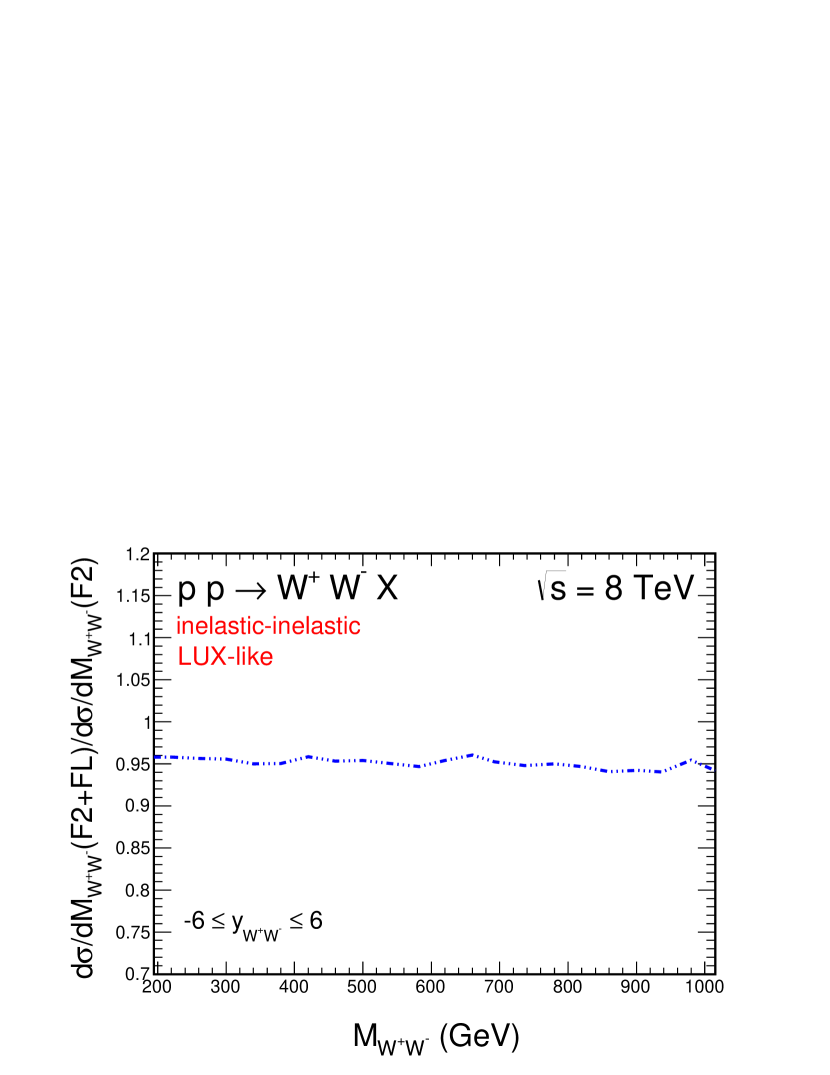
We now wish to discuss the importance of the longitudinal structure function in the photon-flux. This needs some clarification. Arguably the most physical representation of the inelastic flux would be to write the inelastic flux 12 directly in terms of structure functions and . In terms of these structure functions decomposes as , with . If we insert this into Eq.(12), we get positive contributions from as well as . In practice, we have a wealth of experimental data on , and much less knowledge of . It is therefore more practical to express the photon flux directly in terms of and .
We now want to check to which extent the photon fluxes can be evaluated from only. We therefore evaluate the photon flux for two different cases:
In Fig.16 we show the ratio for two different energies. In such a decomposition the cross section when both and are taken into account is smaller by 4-5 % than the cross section when only is taken into account, independent of .

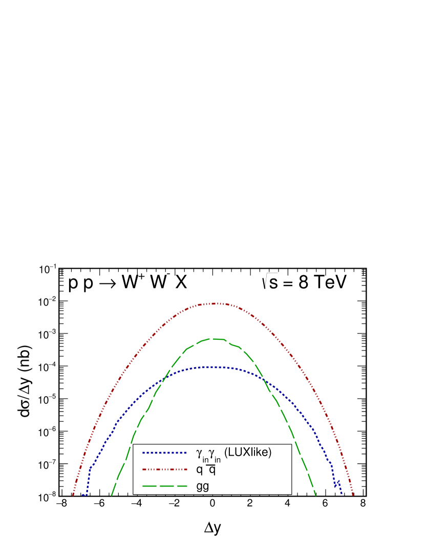
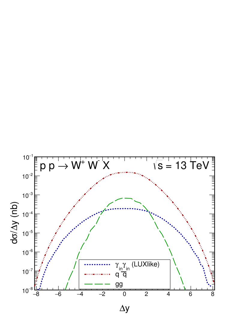
IV.5 Rapidity distance between bosons
The contribution is of the order of 2 % for the inclusive cross section as discussed at the beginning of this section. The technical problem is how to measure the contribution in experiment. This can be done by imposing an extra condition on the size of the rapidity gaps around the electroweak vertex.
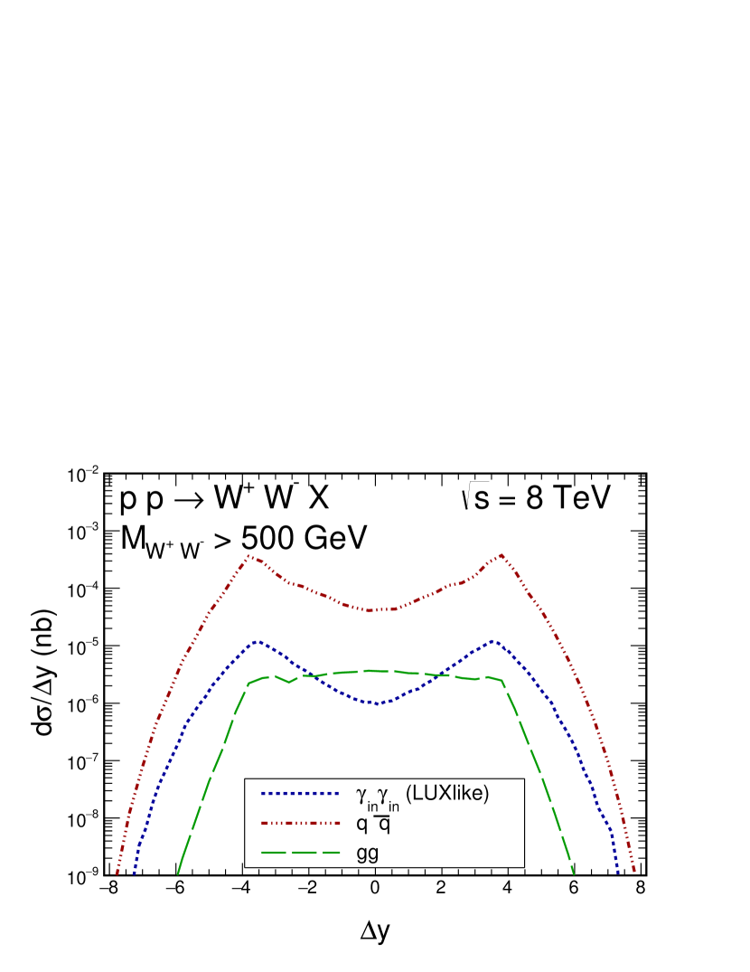
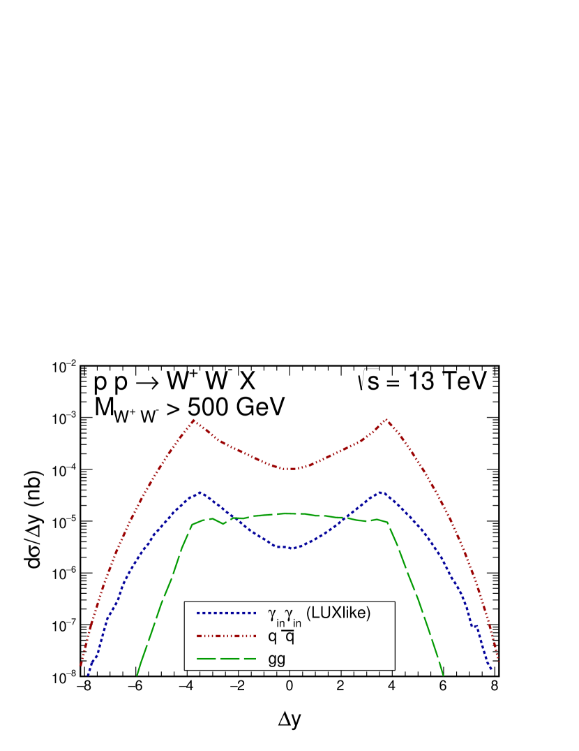
In Fig.17 we show the distribution in the distance in rapidity between the two produced bosons (dotted line) without any extra condition on rapidity gaps. The distribution is fairly flat over several units. This (rapidity distance between muon and electron) can perhaps be used to enhance the data sample for the mechanism. For reference we show also contribution of the annihilation (dash-dotted line) and gluon-gluon fusion (dashed line) which proceed via quark loops. The latter calculation is performed with LoopTools package Hahn:1998yk (for details we refer to LS2013 ). The distribution corresponding to gluon-gluon fusion is much narrower than that of the fusion. It is not so for the quark-antiquark annihilation. The latter is broader due to parton distribution product (, containing valence quarks) as well as due to presence of -channel photon and -boson exchanges. Excluding artificially the latter contributions makes the distribution in much narrower. The distributions change shapes when imposing extra cut on 500 GeV (lower panels), but the general situation is similar.
V Conclusions
In the present paper we have discussed the production of pairs created via the photon-photon fusion mechanism. In contrast to previous approaches we include transverse momenta of photons incoming to the hard process. The matrix elements derived in Nachtmann:2005en have been used. The explicit dependence on polarization state of bosons has allowed us to calculate different polarization contributions.
We have obtained cross section of about 1 pb for the LHC energies. This is about 2 % of the total integrated cross section dominated by the quark-antiquark annihilation and gluon-gluon fusion.
Different combinations of the final states (elastic-elastic, elastic-inelastic, inelastic-elastic, inelastic-inelastic) related to whether the incoming protons do or do not undergo dissociation have been considered. We have focused rather on the dominant inelastic-inelastic component.
The unintegrated photon fluxes were calculated based on modern parametrizations of the proton structure functions from the literature.
Several differential distributions in boson transverse momentum and rapidity, invariant mass, transverse momentum of the pair have been presented and compared with previous results obtained in the collinear approach in LSR2015 . We have obtained a smaller cross section for large invariant masses than in the collinear approximation. Our predictions may be considered as realistic Standard Model reference in searches of effects beyond Standard Model in the process.
Several correlation observables have been studied. Large contributions from the regions of large photon virtualities and/or have been found putting in question the reliability of leading-order collinear-factorization approach. We have found larger virtualities for larger invariant masses of the system. This results seems universal and would be similar e.g. for production of charged Higgs pairs via fusion.
We have found that values (arguments of structure functions) are typically 0.1-0.5. In contrast to the production of charged lepton pairs the production of pairs requires therefore structure functions in the region where they were studied (measured and fitted). The dominant part comes from the region described by the DGLAP evolution equation and only a small fraction comes from nonperturbative region. The nonperturbative contribution (small region) was much larger for the charged lepton production Luszczak:2015aoa where a detailed studies of resonances was necessary.
We have presented a decomposition of the cross section into individual contributions of different polarizations of both bosons. It has been shown that the (both transversally polarized) contribution dominates and constitutes a little bit more than 80 % of the total cross section. The (both longitudinally polarized) contribution is interesting in the context of studying interactions or searches beyond the Standard Model. However, the corresponding cross section is only about 5 %. We have found only a mild dependence of relative amount of different contributions as a function of invariant mass.
We have quantifield the effect of inclusion of longitiudinal structure function into the transverse momentum dependent fluxes of photons. A rather small, approximataly - independent, effect was found.
The discussed here mechanism leads to rather large rapidity separations of and boson. It requires further studies to understand whether it can be used to relatively enhance contribution of the in experimental studies.
Acknowledgments
We are indebted to Piotr Lebiedowicz for providing us a program to calculate gluon-gluon fussion mechanism. This study was partially supported by the Polish National Science Centre grants DEC-2013/09/D/ST2/03724 and DEC-2014/15/B/ST2/02528 and by the Center for Innovation and Transfer of Natural Sciences and Engineering Knowledge in Rzeszów. We are indebted to Laurent Forthomme for discussion of some issues presented here.
References
- (1) V. M. Budnev, I. F. Ginzburg, G. V. Meledin and V. G. Serbo, Phys. Rept. 15, 181 (1975).
- (2) G. G. da Silveira, L. Forthomme, K. Piotrzkowski, W. Schäfer and A. Szczurek, JHEP 1502 (2015) 159 [arXiv:1409.1541 [hep-ph]].
- (3) M. Łuszczak, W. Schäfer and A. Szczurek, Phys. Rev. D 93, no. 7, 074018 (2016) [arXiv:1510.00294 [hep-ph]].
- (4) M. Łuszczak, A. Szczurek and Ch. Royon, JHEP 02 (2015) 098.
- (5) P. Lebiedowicz and A. Szczurek, Phys. Rev. D91 (2015) 095008.
- (6) A. D. Martin, R. G. Roberts, W. J. Stirling and R. S. Thorne, Eur. Phys. J. C 39 (2005) 155 [hep-ph/0411040].
- (7) R. D. Ball et al. [NNPDF Collaboration], Nucl. Phys. B 877 (2013) 290 [arXiv:1308.0598 [hep-ph]].
- (8) C. Schmidt, J. Pumplin, D. Stump and C. P. Yuan, Phys. Rev. D 93 (2016) no.11, 114015 [arXiv:1509.02905 [hep-ph]].
- (9) F. Giuli et al. [xFitter Developers’ Team], Eur. Phys. J. C 77 (2017) no.6, 400 [arXiv:1701.08553 [hep-ph]].
- (10) I. F. Ginzburg and A. Schiller, Phys. Rev. D 57, 6599 (1998) [hep-ph/9802310].
- (11) A. Manohar, P. Nason, G. P. Salam and G. Zanderighi, Phys. Rev. Lett. 117 (2016) no.24, 242002 [arXiv:1607.04266 [hep-ph]].
- (12) A. V. Manohar, P. Nason, G. P. Salam and G. Zanderighi, JHEP 1712 (2017) 046 [arXiv:1708.01256 [hep-ph]].
- (13) E. Chapon, C. Royon and O. Kepka, Phys. Rev. D 81 (2010) 074003 [arXiv:0912.5161 [hep-ph]].
- (14) T. Pierzchala and K. Piotrzkowski, Nucl. Phys. Proc. Suppl. 179-180, 257 (2008) [arXiv:0807.1121 [hep-ph]].
- (15) V. Khachatryan et al. [CMS Collaboration], JHEP 1608, 119 (2016) [arXiv:1604.04464 [hep-ex]].
- (16) M. Aaboud et al. [ATLAS Collaboration], Phys. Rev. D 94, no. 3, 032011 (2016) [arXiv:1607.03745 [hep-ex]].
- (17) W. Kilian, T. Ohl, J. Reuter and M. Sekulla, Phys. Rev. D 93, no. 3, 036004 (2016) [arXiv:1511.00022 [hep-ph]].
- (18) R. L. Delgado, A. Dobado and F. J. Llanes-Estrada, Eur. Phys. J. C 77, no. 4, 205 (2017) [arXiv:1609.06206 [hep-ph]].
- (19) M. Szleper, arXiv:1412.8367 [hep-ph].
- (20) O. Nachtmann, F. Nagel, M. Pospischil and A. Utermann, Eur. Phys. J. C 45, 679 (2006) [hep-ph/0508132].
- (21) J. Alwall et al., JHEP 1407 (2014) 079 [arXiv:1405.0301 [hep-ph]].
- (22) H. Abramowicz, E. M. Levin, A. Levy and U. Maor, Phys. Lett. B 269 (1991) 465.
- (23) H. Abramowicz and A. Levy, hep-ph/9712415.
- (24) P. E. Bosted and M. E. Christy, Phys. Rev. C 77, 065206 (2008) [arXiv:0711.0159 [hep-ph]].
- (25) A. Airapetian et al. [HERMES Collaboration], JHEP 1105, 126 (2011) [arXiv:1103.5704 [hep-ex]].
- (26) K. Abe et al. [E143 Collaboration], Phys. Lett. B 452, 194 (1999) doi:10.1016/S0370-2693(99)00244-0 [hep-ex/9808028].
- (27) A. D. Martin, W. J. Stirling, R. S. Thorne and G. Watt, Eur. Phys. J. C 63, 189 (2009) [arXiv:0901.0002 [hep-ph]].
- (28) A. Szczurek and V. Uleshchenko, Eur. Phys. C12 (2000) 663; Phys. Lett. B475 (2000) 120.
- (29) M. Drees and D. Zeppenfeld, Phys. Rev. D 39, 2536 (1989). doi:10.1103/PhysRevD.39.2536
- (30) S. Chatrchyan et al. [CMS Collaboration], Phys. Lett. B 699, 25 (2011) [arXiv:1102.5429 [hep-ex]].
- (31) G. Aad et al. [ATLAS Collaboration], Phys. Lett. B 712, 289 (2012) [arXiv:1203.6232 [hep-ex]].
- (32) T. Hahn and M. Perez-Victoria, Comput. Phys. Commun. 118 (1999) 153 [hep-ph/9807565].
- (33) P. Lebiedowicz, R. Pasechnik and A. Szczurek, Nucl. Phys. B 867 (2013) 61 [arXiv:1203.1832 [hep-ph]].