Projecting UK Mortality using Bayesian Generalised Additive Models

Abstract

Forecasts of mortality provide vital information about future populations, with implications for pension and health-care policy as well as for decisions made by private companies about life insurance and annuity pricing. Stochastic mortality forecasts allow the uncertainty in mortality predictions to be taken into consideration when making policy decisions and setting product prices. Longer lifespans imply that forecasts of mortality at ages 90 and above will become more important in such calculations.

This paper presents a Bayesian approach to the forecasting of mortality that jointly estimates a Generalised Additive Model (GAM) for mortality for the majority of the age-range and a parametric model for older ages where the data are sparser. The GAM allows smooth components to be estimated for age, cohort and age-specific improvement rates, together with a non-smoothed period effect. Forecasts for the United Kingdom are produced using data from the Human Mortality Database spanning the period 1961-2013. A metric that approximates predictive accuracy under Leave-One-Out cross-validation is used to estimate weights for the ‘stacking’ of forecasts with different points of transition between the GAM and parametric elements.

Mortality for males and females are estimated separately at first, but a joint model allows the asymptotic limit of mortality at old ages to be shared between sexes, and furthermore provides for forecasts accounting for correlations in period innovations. The joint and single sex model forecasts estimated using data from 1961-2003 are compared against observed data from 2004-2013 to facilitate model assessment.

1 Introduction

The future level of mortality is of vital interest to policy makers and private insurers alike, as lower mortality results in greater expenditure on pension payments and higher social care spending. Individuals are living longer due to improved mortality conditions and will reach higher ages in greater number as the post-war baby-boom cohort ages, and thus forecasts of mortality at the oldest ages are becoming more important. However, these remain challenging to produce, as the available mortality data at these ages are sparse and concentrated in the most recent years. The work of Dodd et al. (2018a) in producing the 17^th iteration of the English Life Tables provided a methodology for mortality estimation that combines smoothing based on Generalised Additive Models (GAMs) (Wood, 2006) at the youngest ages with a parametric model at older ages. This paper extends this approach to a forecasting context and introduces period and cohort effects, producing fully probabilistic mortality projections within a Bayesian framework.

2 Mortality Forecasting

2.1 Mortality Rates

The raw materials for stochastic mortality forecasts are data on the number of deaths $d_{xt}$ in year $t$ and age last birthday $x$, and matching population counts $P_{xt}$ derived from census data adjusted for births, deaths and migration in the intervening period. The appropriate exposures to risk, needed for the calculation of mortality rates, can be estimated from these population counts. Most often, the estimated mid-year population totals $P_{x(t+0.5)}$ are used to directly approximate exposures over the whole year $R_{xt}$, under the assumption that births, deaths and migrations occur uniformly throughout the year.

The observed deaths rates $d_{xt}/R_{xt}$ for the United Kingdom for the years 1961, 1981, 2001 and 2013 are displayed in Figure 1, based on data taken from the Human Mortality Database (Human Mortality Database, 2016). The Human Mortality Database uses a more sophisticated method of approximating exposure to risk than that described above, accounting for the distribution of deaths within single years of age (Wilmouth et al., 2017). The plotted mortality rates can be seen to decrease with time, and consistently increase with age beyond early adulthood, as might be expected. The empirical rates appear volatile at higher ages where there are fewer survivors and therefore less data.

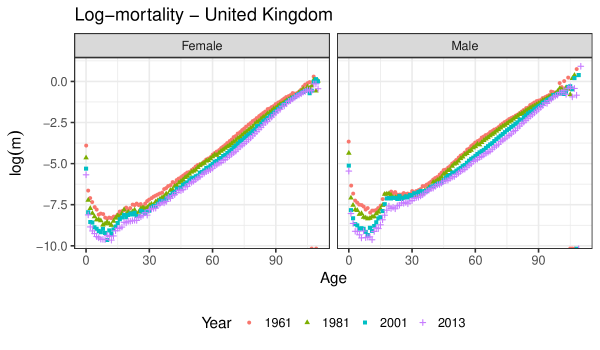
Figure 1: Log-Mortality rates for the United Kingdom for selected years, males and females. Source: Human Mortality Database

The central mortality rate, the quantity which we wish to estimate and forecast, is defined as

$$m_{xt}=\frac{E[d_{xt}]}{R_{xt}}.$$ (1)

This is equal to the force of mortality or hazard of death $\mu(x)$ within the year and age group under the assumption that the force of mortality is constant over that interval. Thatcher et al. (1998) and Keyfitz and Caswell (2005) provide more detail on the exact relationship between these quantities.

2.2 Models of Mortality

A large part of the existing literature on stochastic mortality modelling has developed from the work of Lee and Carter (1992). This approach models the log-mortality rate $\text{log}(m_{xt})$ using an age-specific term $\alpha_{x}$, giving the mean mortality rate for each age $x$, and a bi-linear term $\beta_{x}\kappa_{t}$, where the $\kappa$ vector describes the overall pace of mortality decline, while the $\beta$ coefficients describe how this decline varies by age, so that

$$\text{log}({m_{xt}})=\alpha_{x}+\beta_{x}\kappa_{t}.$$ (2)

This reduces the complexity of the forecasting problem, as only the $\kappa$ component varies over time. This can be modelled using standard Box-Jenkins methods (most often a random walk with drift), which also provide for measures of forecast uncertainty.

The simplicity of the Lee-Carter model has led to a large range of other adjustments and extensions. Brouhns et al. (2002), for example, estimate the parameters through maximisation of a Poisson likelihood for the observed deaths rather than working with a Gaussian likelihood on the log-rates, as in the original paper. Renshaw and Haberman (2003b), in contrast, include multiple bi-linear age-period terms to capture a greater proportion of the total variation than is possible with a single term.

Renshaw and Haberman (2006) go further by adding a cohort term $\beta^{(2)}_{x}\gamma_{t-x}$ to allow for differences in mortality by year of birth. Models that include cohort terms are attractive as in some countries, and notably in the United Kingdom, cohort effects are prevalent in the underlying mortality data, possibly reflecting the different life experiences and lifestyle habits of those born in different periods (Willets, 2004; Cairns et al., 2009). Standard Age-Period-Cohort (APC) models can therefore capture such characteristics of the data, but given the linear dependence in such models (in that $c=t-x$, with $c$ indexing cohort), identifying constraints are needed for fitting.

The work of Cairns and collaborators (Cairns et al., 2009; Dowd et al., 2010) describes a family of models where mortality is modelled through sums of terms of the form $\beta_{x}\kappa_{t}\gamma_{t-x}$, where $\beta_{x}$ refers to age effects, $\kappa_{t}$ to period effects, and $\gamma_{t-x}$ to cohort effects. Any of these elements may be constant or deterministic in particular models, and so the Lee-Carter and Age-Period-Cohort models are incorporated as special cases. The in-sample and forecasting performance of these models are assessed against a number of criteria in Cairns et al. (2009). A notable finding was the lack of robustness of many of the models investigated that included cohort effects; in particular, parameters in such models were found to be sensitive to the fitting period. Furthermore, Palin (2016) has identified some concerns regarding potentially spurious quadratic patterns in cohort effects in several of the models discussed above, caused by variation in mortality improvement rates by age being captured in the cohort effect.

Renshaw and Haberman (2003a) identify commonalities between the Lee-Carter model and their Generalised Linear Model (GLM) approach to mortality modelling focusing on mortality reduction factors. Instead of modelling declines in mortality using a bi-linear term $b_{x}\kappa_{t}$, however, Renshaw and Haberman include a term $b_{x}t$ that is linear in time, simplifying the fitting process. The $b_{x}$ parameters now represent age-specific mortality improvements, where improvements are defined as differences in log-mortality. In as similar vein, and building on the cohort enhancement proposed by Renshaw and Haberman (2006), an Age-Period-Cohort model for Improvements (APCI) has been developed by the Continuous Mortality Investigation (CMI) (Continuous Mortality Investigation, 2016). However, this forces a deterministic convergence to user-specified long-term rates of mortality improvement rather than using time-series methods for forecasting. Richards et al. (2017), however, do provide full stochastic forecasts using the APCI model by fitting time-series models to the period and cohort effects, and also find that this model fits the data better in-sample than either the APC or Lee-Carter models.

The smoothing of mortality rates is important in forecasting applications to avoid roughness in the age profile of log-mortality due to random variation being perpetuated into the future. A number of smoothing models have thus been proposed. Hyndman and Ullah (2007) approach the problem of mortality forecasting from within the functional data paradigm. From a different perspective, Currie et al. (2004) fits a two-dimensional P-spline to mortality, and produces forecasts by extending the spline into the future. The penalisation of differences in the basis function coefficients used in the P-spline method to ensure smoothness in-sample also provides for extrapolation. Although this model fits the data well, forecasts wholly dependent on extrapolation from splines are likely to be over-sensitive to data and trends at the forecast origin.

Bayesian methods are also increasingly being employed for mortality forecasting in order to incorporate prior knowledge about underlying processes, and provide distributions of future mortality risk accounting for multiple sources of uncertainty. Girosi and King (2008) demonstrate methods for mortality forecasting within a Bayesian framework that allow for smoothing the underlying data together with borrowing strength across regions, as well as jointly forecasting cause-specific mortality. Wiśniowski et al. (2015) use the Lee-Carter method for all three components of demographic change (fertility, mortality and migration), again using Bayesian methods to obtain predictive probability distributions.

The method developed in this paper combines elements of many of the approaches above, including allowing for smooth functions of age and cohort, while providing stable estimates of mortality at extreme ages and avoiding some of the problems caused by lack of robustness in parameter estimation discussed above. The model also shares some features with the APCI model of Richards et al. (2017), particularly in the structure of the main part of the model. However, there are some significant points of difference; the model described here applies to the entire age range, and adopts a Bayesian approach to account for all sources of uncertainty.

2.3 Structure

The remainder of the paper is structured as follows: the next section (3) sets out the features of the model used in later sections. Section 4 details the data used and the estimation procedure. Section 5 presents the posterior distributions of the GAM components and provides predictive distributions for log-rate forecasts, and Section 6 displays posterior distributions combined over several alternative models on the basis of in-sample predictive performance, using the method of Yao et al. (2017). Section 7 presents an alternative model where the sexes are fitted jointly, while Section 8 compares out-of-sample performance of the single-sex and joint models, using the years 2004-2013. Section 9 contrasts forecasts from the joint model with those made by the UK Office for National Statistics (Office for National Statistics, 2016), and the final section offers some conclusions and directions for future work.

3 Model Description

3.1 Bayesian Generalised Additive Models

Generalised Additive Models provide a flexible framework for modelling outcomes where the functional form of the response to covariates is not known with certainty, but is expected to vary smoothly. The general form for such models is as follows (Wood, 2006):

$$g(E(y_{i}))=\mathbf{x}_{i}\boldsymbol{\theta}+s_{1}(x_{i1})+s_{2}(x_{i2})+\;...$$

Here, the expectation of the outcome $y$, possibly transformed by link function $g(.)$, is modelled as the sum of a purely parametric part $\mathbf{X_{i}}\boldsymbol{\theta}$ and a number of smooth functions of covariates $s(.)$. A number of possible choices exist for the implementation of the individual smooth functions, but P-splines are chosen in this case. P-splines are appealing because they are defined in terms of strictly local basis functions, with the domain of each function defined by a set of knots spread across the covariate space (Wood, 2006). Following the Bayesian P-splines approach of Lang and Brezger (2001), prior distributions are used to represent a belief that adjacent P-spline covariates $\boldsymbol{\beta}$ will be close to one another. Multivariate normal prior distributions are used, with the covariance matrix constructed from two matrices, $A$ providing a penalty on the first differences of the vector of coefficients $\boldsymbol{\beta}$, and $B$ penalising the null-space of $A$ ensuring that the resulting prior is proper (Wood, 2016):

$$s(x) =\boldsymbol{\beta}^{T}\textbf{b}(x)$$ (3)

$$\boldsymbol{\beta} \sim\text{MVN}\left(\textbf{0},\;\left[\frac{1}{\sigma^{2}_{A}}A+\frac{1}{\sigma_{B}^{2}}B\right]^{-1}\right).$$

3.2 Generalised Additive Models for Mortality Forecasting

The method of mortality forecasting developed in this paper fits a GAM to the majority of the age range, whilst applying separate parametric models to older age groups and to infants. This allows a flexible but smooth fit where the data allow, and imposes some structure on the model where data are sparse, particularly at very high ages. Deaths $d_{xt}$ are considered to follow a negative binomial distribution parameterised in terms of the mean, which in this case is equal to the product of the relevant exposure $E_{xt}$ and expected death rate $m_{xt}$. The dispersion $\phi$ captures additional variance relative to the Poisson distribution:

$$d_{xt} \sim\text{Neg. Binomial}(E_{xt}m_{xt},\;\phi)$$

$$p(d_{xt}|m_{xt},E_{xt},\phi) =\frac{\Gamma(d_{xt}+\phi)}{d_{xt}!\;\Gamma(\phi)}\left(\frac{E_{xt}m_{xt}}{E_{xt}m_{xt}+\phi}\right)^{d_{xt}}\left(\frac{\phi}{E_{xt}m_{xt}+\phi}\right)^{\phi}.$$

An Age-Period-Cohort GAM for the log-mortality improvement ratios $\text{log}(\frac{m_{xt}}{m_{x(t-1)}})$ could be expressed with P-spline based smooth functions for age and cohort improvements, and an additional period component $\kappa$:

$$\text{log}(\frac{m_{xt}}{m_{x(t-1)}})=s_{\beta}(x)+s_{\gamma}^{*}(t-x)+\kappa^{*}_{t}$$ (4)

.

An equivalent expression of this model can be made in terms of mortality rates rather than mortality log-improvement ratios

$$\text{log}(m_{xt})=s_{\alpha}(x)+s_{\beta}(x)t+s_{\gamma}(t-x)+\kappa_{t},$$ (5)

with the cohort and period terms now accumulated versions of their equivalents in the Equation 4. This is the model used in the estimation process. There are now two smooth functions of age: $s_{\alpha}(x)$, which describes the underlying shape of the log mortality curve; and $s_{\beta}(x)$ which describes the pattern of (linear) mortality improvements with age. Knots are spaced on regular intervals in both the age and cohort direction (every 4 years), with 3 knots placed outside the range of the data at either end of the age range, allowing for proper definition of the P-spline at the edge of the data.

In common with other models involving age, period, and cohort elements, constraints are needed in order to identify the different effects because of the linear relationship between the three components. To this end, the cohort component $s_{\gamma}(t-x)$ is constrained so that the first and last components are equal to zero, and the sum of effects over the whole range of cohorts is zero. The period components $\kappa_{t}$ are similarly constrained to sum to zero and to display zero growth over the fitting period. The full set of constraints is thus:

$$\sum^{T}_{t=1}\kappa_{t} =0;\;\sum^{T}_{t=1}t\kappa_{t}=0;$$ (6)

$$\sum^{C}_{c=1}s_{\gamma}(c) =0;\;s_{\gamma}(1)=0;\;s_{\gamma}(\text{C})=0\;,$$

with $C$ here indicating the most recent cohort and $T$ the latest year. These constraints ensure that linear improvements in mortality with time are estimated as part of the $s_{\beta}(x)$ term.

For older ages, a parametric model is adopted due to the sparsity of the data in these regions – the additional structure provided by specifying a parametric form guards against over-fitting and instabilities in this age range:

$$m_{xt}=\frac{\text{exp}(\beta^{old}_{0}+\beta^{old}_{1}x+\beta^{old}_{2}t+\beta^{old}_{3}xt)}{1+\text{exp}(\beta^{old}_{0}-\text{log}(\psi)+\beta^{old}_{1}x+\beta^{old}_{2}t+\beta^{old}_{3}xt)}\;\text{exp}(s_{\gamma}(t-x)+\kappa_{t})$$ (7)

$$\forall x:x\geq x_{old}.$$

A logistic form is used, allowing mortality rates to tend toward a constant $\psi$ as age increases, as in the model in Beard (1963). Such a pattern in mortality at the population level has some theoretical justification, as it can result when heterogeneity (‘frailty’) is applied to rates that follow a log-linear Gompertz mortality model at the individual level, and this frailty is assumed to be distributed amongst the population according to a gamma distribution (Vaupel et al., 1979). In the life-table context, Dodd et al. (2018a) found that the logistic form performed better than the log-linear equivalent when assessed using cross-validation techniques. Linear age and time effects are included in the old-age model, together with an interaction term, and the cohort and period effects are held in common with the model applied to younger ages and are applied multiplicatively to the logistic model.

Constraints are also applied to the parameters of the old age model to ensure that the derivative of the parametric part of the model with respect to age (ignoring the period and cohort effects) is never less than zero; this reflects our prior belief that mortality should not decrease with age after middle-age. The constraints required are as follows, with $H$ describing the most distant time for which forecasts are desired:

$$\beta^{old}_{1} >0$$ (8)

$$\beta^{old}_{2} <0$$

$$\beta^{old}_{3} >-\frac{\beta^{old}_{1}}{\text{H}}\;.$$

Infant mortality is also excluded from the GAM, as it behaves differently from mortality at other ages. The model for infants is given a similar structure to the old age model, except that the period effect $\kappa_{t}$ is excluded, as variation in infant mortality with time does not appear to follow the same pattern as it does over the rest of the age range.

$$\text{log}(m_{0t})=\beta_{1}^{0}+\beta^{0}_{1}t+s_{\gamma}(t)\;.$$ (9)

The period-specific effects $\kappa_{t}$ in Equations 5 and 7 are common across ages and capture deviations from the linear trend described by the smooth improvements $s_{\beta}$. These effects are not modelled as smooth, as they may capture effects such as weather conditions or infectious disease outbreaks that would not be expected to vary smoothly from year to year. The innovations in these period effects $\epsilon$ are given a normal prior with variance $\sigma_{\kappa}$, so that

$$\kappa_{t} =\kappa_{t-1}+\epsilon_{t}$$ (10)

$$\epsilon_{\kappa} \sim\text{Normal}(0,\sigma_{\kappa}^{2})\;.$$

However, these effects are constrained in order to identify the APC model, so we need to account for this by conditioning on the two period constraints given in Equation 6. This is achieved by transforming the $\boldsymbol{\epsilon}$ parameters using a matrix $Z$, constructed so that the final $T-2$ parameters remain unchanged, but the first two transformed parameters will equal zero if the constraints on the cumulative sum of the $\boldsymbol{\epsilon}$ series hold (see Appendix). The resulting vector $\eta$ has a multivariate normal distribution

$$\boldsymbol{\eta} =Z\boldsymbol{\epsilon}$$ (11)

$$\boldsymbol{\eta} \sim\text{Multivarate Normal}(\boldsymbol{0},ZZ^{T}\sigma_{\kappa}^{2}).$$

A distribution conditioning on the first two elements of $\boldsymbol{\eta}$, denoted $\eta_{\dagger}$, equaling zero can be obtained using standard results for the multivariate normal. This conditional prior on $\boldsymbol{\eta^{*}}$ (which contains the last $T-2$ elements of $\boldsymbol{\eta}$) is the distribution used for sampling, and the full set of values of $\boldsymbol{\epsilon}$ can then be recovered deterministically

$$\boldsymbol{\eta} =\begin{bmatrix}\boldsymbol{\eta^{\dagger}}\\ \boldsymbol{\eta^{*}}\end{bmatrix}$$ (12)

$$\boldsymbol{\eta{*}}|(\boldsymbol{\eta^{\dagger}}=\textbf{0}) \sim\text{N}(0,\Sigma_{**}-\Sigma_{*\dagger}\Sigma_{\dagger\dagger}^{-1}\Sigma_{\dagger*})$$

$$\Sigma =ZZ^{T}\sigma_{\epsilon}^{2}$$

$$\boldsymbol{\epsilon} =Z^{-1}\begin{bmatrix}\boldsymbol{0}\\ \boldsymbol{\eta^{*}}\end{bmatrix},$$

where subscripts on the covariance matrices indicate partitions so that $\Sigma_{*\dagger}$ is the sub-matrix of $\Sigma$ with rows corresponding to $\eta^{*}$ and columns to $\eta^{\dagger}$. For forecasts, innovations of the period coefficients are unconstrained and so have independent normal distributions with variance $\sigma_{\kappa}^{2}$.

The same method is used to define a distribution for the innovations in the basis functions coefficients for the cohort spline, accounting for the cohort constraints in Equation 6. In contrast to the period effects, however, the transformation matrix used accounts for the fact that the constraints apply to the resulting smooth function and not the coefficient values themselves. Knots for the basis functions of the cohort smooth are evenly spaced along the range of cohorts to be estimated, so forecasts of future cohort values can be obtained by drawing new coefficient innovations from the normal distribution with mean zero and variance $\sigma_{\gamma}^{2}$. Full details are given in the appendix.

Priors for the model hyper-parameters are generally vague, although not completely uninformative:

$$\beta^{old} \sim\text{Normal}(0,100)$$

$$\beta^{0} \sim\text{Normal}(0,100)$$

$$\sigma_{A} \sim\text{Normal}_{+}(0,100)$$

$$\sigma_{B} \sim\text{Normal}_{+}(0,100)$$

$$\sigma_{\kappa} \sim\text{Normal}_{+}(0,100)$$

$$\sigma_{\gamma} \sim\text{Normal}_{+}(0,100)$$

$$\phi \sim U(-\infty,\infty)$$

$$\psi \sim\text{Log Normal}(0,1).$$

The adoption of weakly informative priors aims to capture something about the expected scale and location of the parameters in question; this aids convergence of the Monte Carlo Markov Chain (MCMC) samples, but with reasonable amounts of data should not affect the final inference to any great extent (Gelman et al., 2014). The scale of the data and covariates is also important in determining the interpretation of these priors; the use of standardised age and time indexes means that regression coefficients are unlikely to take large values. The use of addition symbol as a subscript appended to the normal distribution, $\text{Normal}_{+}$, indicates that only the positive part of the normal distribution is used, therefore referring to a half-normal distribution.

4 Estimation

Samples from the posterior distributions of the parameters and rates were drawn using Hamiltonian Monte Carlo (HMC) and specifically using the stan software package (Stan Development Team, 2015). Stan and its interface in the R programming language (R Development Core Team, 2017) allows the construction of a HMC ‘No U-turns Sampler’ (NUTS) (Hoffman and Gelman, 2014) from a simple user specification of the Bayesian model to be estimated. The code required to fit the model is provided in the supplementary materials for this paper. HMC is a special case of the more general Metropolis-Hastings algorithm for Markov Chain Monte-Carlo sampling, and uses the derivatives of log-posterior with respect to the parameters of interest in the sampling process, often allowing the posterior to be traversed much more quickly than is the case under standard methods (Neal, 2010). The model was fitted using Human Mortality Database data for the UK from 1961–2013 (Human Mortality Database (2016)). The first five cohorts (those born before 1856) are excluded, as exposures are very low for these groups. Four parallel chains were constructed, each with 8000 samples, and the first half of each chain was used as a warm-up period (during which stan tunes the algorithm to best reflect the characteristics of the posterior) and discarded. Parallel chains were used to better assess convergence to the posterior distribution; the diagnostic measure advocated by Gelman and Rubin (1992) indicates that all parameters have converged to an acceptable degree. The 16000 post-warm-up samples were ‘thinned’ by a factor of 4 by discarding three values in four to avoid excessive memory usage, leaving 4000 posterior samples for inference for each model.

5 Initial Results

Some preliminary results are displayed in this section, conditional on a particular choice for the point of transition between the GAM to the parametric old-age model. Fitting a similar model to ONS data for England and Wales for 2010-2012, Dodd et al. (2018a) found using cross-validation methods that the most probable points of transition were age 91 for females and 93 for males. Samples were obtained for models using these transition points, and the posterior distributions of the parameters of the GAM model are given in Figures 2 and 3 for males and females respectively. The colour scheme in these plots identifies intervals containing various proportions of the posterior density, so that the deepest red represents the central 2% interval, whilst 90% of the posterior density is contained between the lightest pink bands. The distributions of mortality improvement rates for both males and females display greater uncertainty at younger ages where there are fewer deaths. As might be expected, uncertainty for cohort effects increases for the oldest and most recent cohorts, as these have the fewest data-points. Note that it is the differenced cohort and period effects ($s_{\gamma}^{*}(t-x)$ and $\kappa^{*}_{t}$ from Equation 4) that are plotted rather than their summed equivalents.

Differences between the sexes are most notable in the age-specific component, for which the accident hump for young males is more prominent, and in the improvement rates, for which males show lower rates of improvement than females in their late 20s. Cohort and period contributions to mortality decline show similar but not identical patterns for each sex.

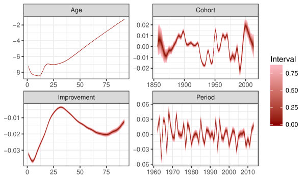
Figure 2: GAM components, males, transition point=93

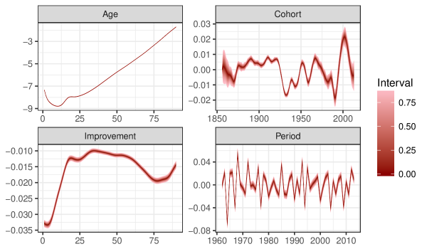
Figure 3: GAM Components, females, transition Point=91

Posterior distributions for log rates generated from this model fit the data relatively closely. However, Figure 4 displays forecasts at fifty years into the future, which, while appearing reasonable, contain a small discontinuity in the distribution of log rates, particularly visible for males, at the point of transition between the GAM and the parametric model. This suggests that some sort of averaging over or combination of models using different transition points might be advisable.

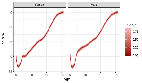
Figure 4: Predictive distribution of log rates using single points of transition, 2063

6 Transition Points and Model Stacking

The choice made regarding the age at which the model transitions from the GAM (used over the majority of the age range) to the parametric model for old ages is essentially arbitrary; we do not believe that there is a switch between data-generating processes at some point $x_{old}$, but rather that the task of predicting mortality is better served by two models. There is thus no ‘true’ value for the point of transition, and decisions regarding transition should be governed by model performance. The methodology used in the latest English Life Tables (Dodd et al., 2018a) used cross-validation to obtain posterior weights over a set of models $M$ defined by $K$ different points of transition, based on mortality data from 2010–2012. In that analysis, age 91 for females and 93 for males are the most probable points of transition, and the final predictive distribution was obtained by averaging over models using the calculated weights. However, the model described here differs to that used in Dodd et al. (2018a) in that it varies in time and applies to a period spanning many years, so the question of the distribution of the transition between the parametric model and the GAM must be revisited.

Separate models were therefore estimated for transition points ranging from 80 to 95, and their accuracy was assessed using the Leave-One-Out Information Criteria, (LOOIC), developed by Vehtari et al. (2015). LOOIC is a measure of how well we might expect a model to perform in predicting a data-point without including it in the data used to fit the model. It is based on an approximation of the Leave-One-Out (LOO) log point-wise predictive density $\sum^{n}_{i=1}\text{log}\;p(y_{i}|y_{-i})$, where the $y_{-i}$ subscript indicates a data-set excluding the $i$th observation, $\theta$ is a vector of parameters, and:

$$p(y_{i}|y_{-i})=\int p(y_{i}|\theta)p(\theta|y_{-i})d\theta\;.$$

Rather than fitting the model $n$ times (once for every data-point), Vehtari et al. (2015) provide a method for approximating the LOOIC from just one set of posterior samples of the predictive density computed from the full data-set, implemented within the loo R package. This uses importance sampling to approximate the LOO log-predictive density, correcting for instabilities caused by high or infinite variance of the importance weights by fitting a Pareto distribution to the upper tail of the raw weights.

The LOOIC scores for males and females for the models with transition points $k=[80,81,...,95]$ are given below in Figure 5. Later cut-points tend to be preferred because the greater flexibility of the GAM model gives higher LOOIC values even at relatively high ages, although the absolute differences between the models are small. Models with points of transition above age 95 are not considered, as this would leave too few data-points with which to estimate the old-age model effectively.

Although LOOIC is not a measure of forecast performance as such, as it is focused on how the model would perform at predicting data-points contained within the original data-set and does not consider the times at which data-points become available, it does provide an indication of how well the specified models reflect the structure of the data.

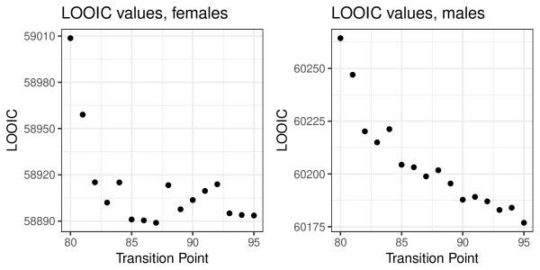
Figure 5: LOOIC values for models using different transition points

Following the work by Yao et al. (2017), these LOOIC values can be used for as the basis for ‘stacking’ the predictive distributions of each model to obtain a distribution which combines models in a principled way, with weights determined by approximate cross-validation performance. Stacking is often used for averaging over point estimates in ensemble models, but Yao et al. (2017) extend the approach to apply to combining distributions. More specifically, the weights $\boldsymbol{w}$, elements of which corresponding to one of $K$ possible models $M_{k}$, are estimated through the solution of the optimisation problem

$$\underset{\boldsymbol{w}}{\operatorname{argmax}}\sum_{i=1}^{n}\text{log}\left(\sum_{k=1}^{K}w_{k}\;p(y_{i}|y_{-i},M_{k})\right)$$ (13)

$$\text{s.t.}\;w_{k}>0;\;\sum_{k=1}^{K}w_{k}=1\;.$$

(Yao et al., 2017, p.7), where $p(y_{i}|y_{-i},M_{k})$ is approximated using the LOOIC measure described above. The form of the combined predictive distribution is then $\hat{p}(\tilde{y}|y)=\sum_{k=1}^{K}w_{k}p(\tilde{y}|y,M_{k})$. The estimated model weights are shown in Figure 6; the greatest individual weight is given to models with the latest points of transitions, reflecting the pattern in the LOOIC measure. Other models with earlier transition points are also given weight, however, reflecting that they perform well at predicting some data-points which are not so well estimated by the late-transition model.

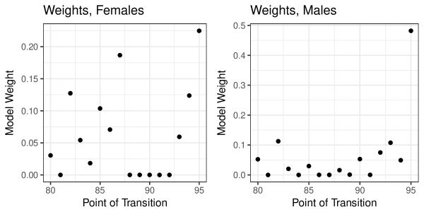
Figure 6: LOOIC values for models using different points of transition

Samples from the combined posterior predictive distribution were obtained using the estimated weights by sampling from the posterior distribution associated with each model in proportion to its weight. The resulting stacked forecasts are given below in Figure 7; the discontinuities seen previously are now smoothed out through the process of taking the weighted combination of distributions.

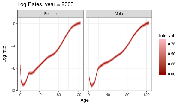
Figure 7: Stacked forecasts for 2063, single-sex models

7 Jointly modelling male and female mortality

In the work described above, models for males and females are estimated separately. However, much of what drives the underlying processes of mortality and how it changes over time is likely to be common between sexes. Thus, we may gain from borrowing strength across models and also from explicitly representing covariances between parameters for each sex, as in Wiśniowski et al. (2015). Because males tend to die sooner than females, there are fewer data-points (that is, lower total exposure) with which to estimate parameters in the old-age model. For this reason, the parameter $\psi$, representing the asymptote of the logistic function in the old-age model, is now shared between sexes.

We also allow the innovations in the period effects $\kappa_{t}$ to be correlated, so that that joint forecasts can be generated accounting for the fact that in potential futures where mortality for females is high, it will tend to be high for males as well. The joint distribution for the period innovations for both sexes, conditional on the constraints, is obtained in a similar way as for the single-sex models, described in Section 3. Full details are given in the appendix.

As before, LOOIC scores and model weights are obtained for the joint model (Figure 8). The pattern of LOOICs and weights are similar to those for the separate models, with the highest transition point obtaining most weight, but considerable weight also attached to earlier transitions.

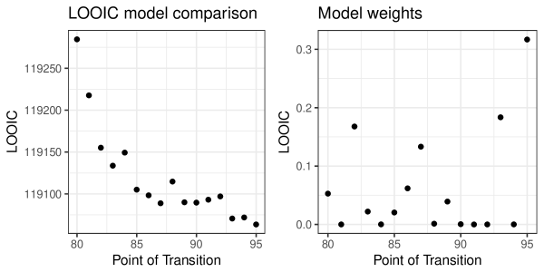
Figure 8: LOOIC and model weights, joint-sex model

Joint forecasts of log-mortality are displayed in Figure 9. The estimated correlation in the innovations of the period effects (the off-diagonal elements of $P$) is high - generally above 95%.

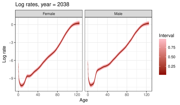
Figure 9: Stacked forecasts from joint-sex model, 2038

8 Model Assessment

In order to assess the robustness and forecasting accuracy of the models described above, fitting was conducted on a truncated data-set, excluding the years 2004-2013. Robustness was then assessed by comparing posterior means of the main smooth functions estimated on this reduced data-set against the same quantities estimated on all the data. Figure 10 displays such a comparison for males, plotting posterior means for each point of transition and fitting period. Estimates of period and cohort effects are relatively stable, particularly in the interior of the data. While some differences are evident in the pattern of improvements, the general shape of the curve is notably similar, and the downward shift appears to reflect real increases in the rate of mortality decline after 2003, particularly for younger adults. The shape of the age effect is again very similar, and the differing location of the smooth curve is accounted for by a change in the location of the intercept of the time index in Equation 5 for different data periods.

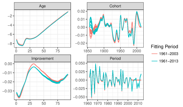
Figure 10: Comparison of posterior means of GAM model components for different fitting periods and transition points, males

Both the single and joint-sex models presented above appear to give reasonable forecasts for future mortality. Figures 11 and 12 display predictive distributions and empirical rates for younger and older ages respectively. Comparing the predictive posterior distributions against the observed outcomes, it is evident that for most of the age range, empirical rates fall within the 90% predictive interval. The exception is young adult males, between the ages of about 15 and 40, for whom recent drops in mortality far outpace those seen in the observed data 1961-2003. More formal assessments of forecast performance are difficult, as we observe only one correlated set of outcomes (that is, male and female log-rates 2004-2013).

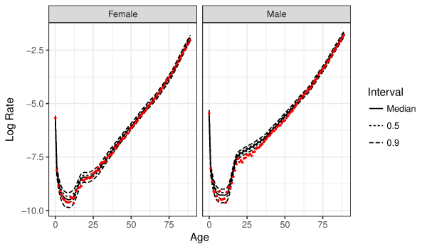
Figure 11: Comparison of posterior predictive distributions for log-rates against empirical observations, 2013, joint-sex model.

Focusing on older ages (Figure 12), we can see that there are few differences between the predictive distributions of the joint- and single-sex models, and those that are evident occur only at high ages. In part, this may be because the weighting procedure works to select models with similar properties. Other considerations may be taken into account when deciding between the two models; the joint model is more parsimonious in that fewer parameters are required to fit it, and it allows for correlations in the paths of mortality by sex to be taken into account. In contrast, the single sex model is less computationally demanding, particularly with respect to memory, as each sex is fitted and processed separately.

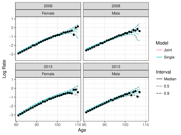
Figure 12: Comparison of posterior predictive distributions for old-age log-rates against empirical observations, 2008 and 2013, single and joint-sex models.

9 Comparison to offical projections and variants

The final stacked forecast from the joint model in the previous section are now compared with forecasts produced by the United Kingdom Office for National Statistics (ONS) in the 2014-based National Population Projections (NPP) (Office for National Statistics, 2016). These work with the predicted probabilities of deaths $q_{x}$ rather than the central mortality rates $m_{x}$; the former represents the probability of dying by age $x+1$ given that an individual attains age $x$. Posterior predictive samples of $q_{xt}$ were acquired using the approximation

$$q_{xt}\approx 1-\text{exp}(-m_{xt}).$$ (14)

As well as the principal ONS projection from the 2014-based NPP, the variant projections involving high and low mortality scenarios have been included, allowing some understanding of how the existing indications of uncertainty resulting from different projection assumptions compare with the fully Bayesian probability distributions.

Figure 13 shows posterior distributions of log-transformed death probabilities $q_{x}$ for a forecast horizon of 25 years for both males and females, together with the equivalent $q_{x+0.5}$ quantities for the same year (2038) obtained from the ONS 2014-based NPP. For most of the age range, the forecasts are similar, with the principal projection falling close to the median prediction under the GAM-based model. However, the ONS model projects lower mortality for young adults for both sexes, to the extent that the principal projections fall outside the outermost 90% predictive interval of the probabilistic projections. This is due to a greater weight given by the ONS methodology to more recent high improvement rates at these ages (see Office for National Statistics, 2016, for more details regarding the ONS methodology).

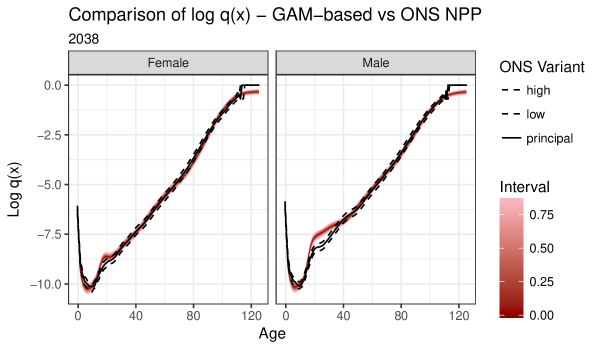
Figure 13: Forecast log-probabilities of death for 2038

9.1 Life Expectancy

Period life expectancy at birth is a useful summary measure of the mortality conditions in a given year. It captures the expected number of years lived of a hypothetical individual who experiences a given period’s schedule of mortality rates over the course of their whole life. Figure 14 compares the posterior distribution of life expectancy at birth ($e_{0}$) from the jointly fitted GAM-based model with the equivalent quantity from the NPP. The GAM-based forecasts appear more optimistic than the ONS equivalent, with median life expectancy higher than the principal ONS projection due to the lower predictions of mortality at ages 70-95 under the GAM-based model. Figure 14 also reveals that uncertainty in $e_{0}$ initially grows more quickly in the Bayesian approach developed above, in that the gap between the high and low variants is much narrower than the fan intervals for at least the first decade of the forecast. After 30 years, however, the range spanned by the ONS variants becomes wider than 90% probabilistic interval from the GAM-based model. The uncertainty in the probabilistic forecast reflects past variability in the observed data, and from the comparison with hold-back data given in Figures 11 and 12, the calibration of this uncertainty appear reasonable. As a result, we believe that the probabilistic intervals provide a better indication of the uncertainty around future life expectancy than the scenario-based equivalents, at least in the short term, particularly as they have a readily understandable interpretation in terms of probability.

Figure 14: Forecast Life Expectancy at Birth, ONS NPP and GAM-based forecast

10 Discussion and Conclusion

This paper details methodology for the fully probabilistic forecasting of mortality rates, accounting for uncertainty in parameter estimates as well as in forecasting. The approach uses a GAM to produce smooth rate estimates at younger ages, and combines this with a parametric model at higher ages where the data are more sparse, allowing rate estimates to be obtained for extreme old ages. The use of Hamiltonian Monte Carlo sampling and the stan software package allowed posterior sampling to be conducted with reasonable efficiency.

Stacking predictive distributions following the approach of Yao et al. (2017) provides a principled approach to avoiding a single choice of transition point between these two sub-models governing younger and older age ranges. These weights are based on approximate Leave-One-Out cross-validation performance, and thus weight models based on their ability to predict data contained in the original fitting period. An alternative approach may be to fit models on a subset of data, and produce weights based on model performance in forecasting data at the end of the time period. However, this would involve additional model refitting, and it may also be the case that such assessments are overly sensitive to characteristics of the held-out data. Furthermore, log-scores based on a single set of observed outcomes are likely to be highly correlated, and thus rolling n-step-ahead forecasts may be required to assess forecast performance robustly, which would necessitate repeated model fitting with even greater computational expense.

A comparison with ONS forecasts provides an indication of how Bayesian predictive intervals compare with the deterministic scenario-based indicators of forecast variability produced by ONS. For life expectancy in particular, the probabilistic intervals are considerably wider over a short time horizon than those suggested by the high and low mortality scenarios. Future work could investigate the inclusion of expert opinion in probabilistic mortality forecasting models like the one presented in this paper. The NPP uses experts to provide target rates of mortality improvement over longer time horizons (25 years) (Office for National Statistics, 2016), reflecting the fact that extrapolative methods may prove inferior to expertise at this distance into the future. A similar approach within a Bayesian framework would have to consider that using expert opinion about future rates is different from the standard approach of eliciting information about model parameters directly. Work in Dodd et al. (2018b) describes one way in which this could be achieved. Beyond this, there are also opportunities to investigate the possibility of extending similar methods to other demographic components, particularly fertility.

References

- (1)
- Beard (1963) Beard, R.: 1963, A theory of mortality based on actuarial, biological, and medical considerations., Proceedings of the International Population Conference1, International Union for the Scientific Study of Population, New York, pp. 611–625.
- Brouhns et al. (2002) Brouhns, N., Denuit, M. and Vermunt, J. K.: 2002, A Poisson log-bilinear regression approach to the construction of projected lifetables, Insurance: Mathematics and Economics 31(3), 373–393.
- Cairns et al. (2009) Cairns, A. J. G., Blake, D., Dowd, K., Coughlan, D., Epstein, D. and Ong, A.: 2009, A Quantitative Comparison of Stochastic Mortality Models Using Data from England and Wales and the United States, North American Actuarial Journal 13, 1–35.
-
Continuous Mortality Investigation (2016)
Continuous Mortality Investigation: 2016, CMI Mortality Projections Model
consultation.
https://www.actuaries.org.uk/documents/cmi-working-paper-90-cmi-mortality-projections-model-consultation - Currie et al. (2004) Currie, I. D., Durban, M. and Eilers, P. H. C.: 2004, Smoothing and forecasting mortality rates, Statistical Modelling 4, 279–298.
-
Dodd et al. (2018a)
Dodd, E., Forster, J. J., Bijak, J. and Smith, P. W. F.: 2018a, Smoothing
mortality data: the English Life Tables , 2010-2012, Journal of the
Royal Statistical Society: Series A (Statistics in Society) Early
View.
http://doi.wiley.com/10.1111/rssa.12309 - Dodd et al. (2018b) Dodd, E., Forster, J. J., Bijak, J. and Smith, P. W. F.: 2018b, Stochastic Modelling and Projection of Mortality Improvements Allowing for Overdispersion, Working Paper.
-
Dowd et al. (2010)
Dowd, K., Cairns, A. J. G., Blake, D., Coughlan, G. D., Epstein, D. and
Khalaf-Allah, M.: 2010, Evaluating the goodness of fit of stochastic
mortality models, Insurance: Mathematics and Economics 47(3), 255–265.
http://dx.doi.org/10.1016/j.insmatheco.2010.06.006 - Forster et al. (2016) Forster, J. J., Dodd, E., Bijak, J. and Smith, P. W. F.: 2016, A Comprehensive Framework for Mortality Forecasting, Joint Eurostat/UNECE Work Session on Demographic Projections, Geneva.
- Gelman et al. (2014) Gelman, A., Carlin, J. B., Stern, H. S., Dunson, D. B., Vehtari, A. and Rubin, D. B.: 2014, Bayesian Data Analysis, third edn, CRC Press, Abingdon.
- Gelman and Rubin (1992) Gelman, A. and Rubin, D. B.: 1992, Inference from Iterative Simulation Using Multiple Sequences, Statistical Science 7(4), 457–472.
- Girosi and King (2008) Girosi, F. and King, G.: 2008, Demographic Forecasting, Princeton Univeristy Press, Princeton.
-
Hoffman and Gelman (2014)
Hoffman, M. D. and Gelman, A.: 2014, The no-U-turn sampler: Adaptively setting
path lengths in Hamiltonian Monte Carlo, Journal of Machine Learning
Research 15(2008), 1–31.
http://arxiv.org/abs/1111.4246 -
Human Mortality Database (2016)
Human Mortality Database: 2016, Human Mortality Database.
http://www.mortality.org/cgi-bin/hmd - Hyndman and Ullah (2007) Hyndman, R. J. and Ullah, M. S.: 2007, Robust forecasting of mortality and fertility rates: A functional data approach, Computational Statistics and Data Analysis 51(10), 4942–4956.
- Keyfitz and Caswell (2005) Keyfitz, N. and Caswell, H.: 2005, Applied Mathematical Demography, third edn, Springer, New York.
-
Lang and Brezger (2001)
Lang, S. and Brezger, A.: 2001, Bayesian P-Splines.
https://epub.ub.uni-muenchen.de/1617/ -
Lee and Carter (1992)
Lee, R. D. and Carter, L. R.: 1992, Modeling and Forecasting U.S Mortality,
Journal of the American Statistical Association 87(419), pp.
659–671.
http://www.jstor.org/stable/2290201 - Neal (2010) Neal, R.: 2010, MCMC using Hamiltonian Dynamics, in S. Brooks, A. Gelman, G. Jones and X.-L. M. Meng (eds), Handbook of Markov Chain Monte Carlo, Chapman and Hall / CRC Press.
-
Office for National
Statistics (2016)
Office for National Statistics: 2016, National Population Projections:
2014-based Reference Volume, Series PP2, Technical report, Office for
National Statistics.
https://www.ons.gov.uk/peoplepopulationandcommunity/populationandmigration/populationprojections/compendium/nationalpopulationprojections/2014basedreferencevolumeseriespp2 -
Palin (2016)
Palin, J.: 2016, When is a cohort not a cohort ? Spurious parameters in
stochastic longevity models, International Mortality and Longevety
Symposium, London.
https://www.actuaries.org.uk/documents/c2-when-cohort-not-cohort-spurious-parameters-stochastic-longevity-models -
R Development Core Team (2017)
R Development Core Team: 2017, R: A Language and Environment for Statistical
Computing.
http://www.r-project.org/ -