Diffusion of Elements in the Interstellar Medium in Early-Type Galaxies

Abstract

We consider the role of diffusion in the redistribution of elements in the hot interstellar medium (ISM) of early-type galaxies. It is well known that gravitational sedimentation can affect significantly the abundances of helium and heavy elements in the intracluster gas of massive galaxy clusters. The self-similarity of the temperature profiles and tight mass–temperature relation of relaxed cool-core clusters suggest that the maximum effect of sedimentation take place in the most massive virialized objects in the Universe. However, Chandra and XMM-Newton observations demonstrate more complex scaling relations between the masses of early-type galaxies and other parameters, such as the ISM temperature and gas mass fraction. An important fact is that early-type galaxies can show both decreasing and increasing radial temperature profiles. We have calculated the diffusion based on the observed gas density and temperature distributions for 13  early-type galaxies that belonging to the different environments and cover a wide range of X-ray luminosities. To estimate the maximum effect of sedimentation and thermal diffusion, we have solved the full set of Burgers’ equations for a non-magnetized ISM plasma. The results obtained demonstrate a considerable increase of the He/H ratio within one effective radius for all galaxies of our sample. For galaxies with a flat or declining radial temperature profile the average increase of the helium abundance is 60% in one billion years of diffusion. The revealed effect can introduce a significant bias in the metal abundance measurements based on X-ray spectroscopy and can affect the evolution of stars that could be formed from a gas with a high helium abundance.

1 Introduction

The role of diffusion in shaping the spatial distribution of elements in the intracluster medium (ICM) of galaxy clusters has been the subject of many previous studies (Fabian & Pringle, 1977; Gilfanov & Syunyaev, 1984; Chuzhoy & Loeb, 2004; Peng & Nagai, 2009a; Shtykovskiy & Gilfanov, 2010; Medvedev et al., 2014). In the approximation of a non-magnetized ICM plasma the diffusion is driven by the gravity, concentration and temperature gradients. In particular, large temperature gradients in cool-core clusters slow down the sedimentation of elements heavier than hydrogen at the cluster center. Given the observed self-similar ICM temperature profile in relaxed clusters (Vikhlinin et al., 2006), it can be asserted that the integrated effect of diffusion depends mainly on the global properties of the clusters: the total mass ($M$), the mean temperature ($T$), and the gas mass fraction ($f_{b}$). However, these parameters are not independent. Observations (Vikhlinin et al., 2006) revealed a tight correlation between the cluster temperature and total mass, in agreement with expected on theoretical grounds (see, e.g., Mathiesen & Evrard, 2001). At the same time, the enclosed baryon fraction in clusters is expected to be close to the cosmic mean (White et al., 1993), which is also confirmed by observations (Vikhlinin et al., 2006). The small scatter of values in the relations suggests a similar galaxy cluster formation history. Thus, one may talk about an explicit dependence of the sedimentation amplitude on cluster mass and expect a maximum effect for the most massive (hot) virialized objects.

In this paper we consider the elements diffusion in the interstellar medium (ISM) in early-type (elliptical and lenticular) galaxies. Although the total mass, temperature, and gas mass fraction are also correlated for such objects, there is a large scatter at a fixed value of any parameter. It is also important that no “universal” temperature profile is observed for early-type galaxies: the ISM can have both decreasing and increasing with radius temperature profiles. This can affect significantly the sedimentation amplitude.

The scatter in observed X-ray properties can be partly related to the difficulty of studying the emission from the ISM. It is often challenging to disentangle relatively weak ISM emission from the strong emission of surrounding ICM gas. X-ray spectroscopy of low-luminosity galaxies runs into the problem of a too small signal-to-noise ratio. Yet another difficulty in studying such objects is related to the necessity of separating the diffuse thermal X-ray emission of the ISM from the emission of the galactic stellar population (low-mass X-ray binaries and cataclysmic variables) and occasionally also the emission of the central supermassive black hole. On the other hand, by now dozens of early-type galaxies have been observed with Chandra and XMM-Newton, and, hence, a large volume of sufficient quality data has been accumulated. The unprecedented Chandra angular resolution and the high XMM-Newton sensitivity allow the gas temperature and density to be obtained in a uniform way for the entire sample of galaxies being studied.

The mass–temperature relation demonstrates a more complex behaviour for early-type galaxies (Boroson et al., 2011) than does the virial relation, $M\sim T^{3/2}$, which is closely followed by the measured relation for galaxy clusters (adjusted for the same redshift). Besides, the measured gas temperatures in such galaxies always turn out to be higher than the virial values. This suggests the importance of additional gas heating sources, apart from the heating by adiabatic compression during infall in the galactic gravitational potential and the thermalization of the gas kinetic energy associated with random stellar motions (see Pellegrini, 2011). The explosions of SNe Ia and the accretion of gas onto a central supermassive black hole can be such additional heating mechanisms (see, e.g., Ciotti et al., 1991). The contribution of additional heating sources to the overall gas thermal balance changes with galaxy mass. This is observed as a change of the slope in the $\sigma_{c}-T$ relation for galaxies with different luminosities: the faintest galaxies deviate more strongly from the virial relation (Pellegrini, 2011). Note that the central velocity dispersion, $\sigma_{c}$, is believed to be a representative measure of the galactic potential well (O’Sullivan et al., 2003); therefore, one may talk about similar features in the $M-T$ relation.

In the case of galaxy clusters, the baryon fraction $f_{b}$ approaches the cosmological value within a radius $r\sim r_{500}$(within which the mean density exceeds the critical density of the Universe by a factor of 500). Since the accessible region of observations of early-type galaxies is considerably smaller than $r_{500}$, it is hard to judge the universal value of $f_{b}$. Measurements of the density of the ISM show a smaller gas mass fraction in the accessible region of observations. This is partly due to the much larger mass fraction of stars in galaxies than in clusters. This also can lead to a significant increase of the diffusion efficiency in such objects.

The low observed metallicity of the ISM (Su & Irwin, 2013) remains an important issue in understanding the history of the star formation and evolution of early-type galaxies. Since the red giant winds, planetary nebulae, and supernova explosions serve as the main suppliers of the ISM gas, the heavy-element abundances in the gas are expected to be at least solar. Apart from its direct influence on the heavy-element distribution, diffusion may lead to considerable changes in the helium abundance profile. Therefore, the assumption about a solar helium abundance in analyzing the X-ray spectra can lead to a significant bias in the measured metal abundance (Ettori & Fabian, 2006; Markevitch, 2007; Medvedev et al., 2014). Interestingly, an enhanced helium abundance compared to the cosmological value could result from diffusion already at the galaxy formation stage, but this effect could not exceed a few tenths of a percent (Medvedev et al., 2016).

In this paper we calculate the diffusion of elements in the ISM gas based on Chandra  and XMM-Newton observational data. We consider an idealized problem: without magnetic fields and a deviation of the ISM from hydrostatic equilibrium, and with a constant (in time) temperature profile. The goal of this exercise was to estimate the role of diffusion among other physical processes in a hot ISM plasma. By solving the full set of Burgers equations, we demonstrate a nontrivial dependence of the integrated effect on galaxy mass and surrounding environment.

2 The sample of galaxies

Table 1: The early-type galaxies selected for diffusion calculations. The morphological type was taken from NED, $D$ is the distance to the galaxy from Tonry et al. (2001) (the method of surface brightness fluctuations, SB1200F), $r_{\rm eff}$ is the effective radius from the RC3 catalogue (de Vaucouleurs et al., 1991), $L_{X}$ is the deprojected luminosity of the thermal emission within $4\,r_{\rm eff}$ in the soft X-ray range 0.3–2 keV from Nagino & Matsushita (2009) recalculated for the distances from column 3, $M_{\rm ISM}$ is the mass of the interstellar gas within $4\,r_{\rm eff}$, $M_{\rm tot}$ is the total mass within $10\,r_{\rm eff}$ found from Eq. 7, classification of galaxy environments is based on (Faber et al., 1989): 0 for galaxies in the field, 1 for galaxies in groups and clusters, and 2 for galaxies at group center.

Galaxy	Morphological	$D$,	$r_{\rm eff}$,	$L_{X}$,	$M_{\rm ISM}$,	$M_{\rm tot}$,	Environment
	type	Mpc	kpc	$10^{40}$  erg s-1	$10^{8}\,M_{\sun}$	$10^{11}\,M_{\sun}$
IC 1459	E3–4	29.2	4.9	2.1	9.6	14.0	1
NGC 720	E5	27.7	4.8	4.4	11.0	12.0	0
NGC 1316	SAB0	21.5	8.4	5.7	27.0	29.7	1
NGC 1332	S0	22.9	3.1	1.8	2.7	7.4	2
NGC 1395	E2	24.1	5.7	3.2	11.4	19.2	1
NGC 1399	E1	20.0	3.9	13.5	17.7	14.2	2
NGC 3923	E4–5	22.9	5.5	3.8	11.7	11.7	1
NGC 4472	E2	16.3	8.2	21.4	58.0	31.9	2
NGC 4552	E0–1	15.3	2.2	3.3	2.4	6.3	1
NGC 4636	E0–1	14.7	6.3	20.3	25.9	27.8	2
NGC 4649	E2	16.8	5.6	9.9	17.0	21.9	1
NGC 5044	E0	31.2	8.1	166.1	164.7	45.5	2
NGC 5846	E0–1	24.9	7.6	37.9	70.0	92.4	2

To investigate the diffusion, we use 13  galaxies from Nagino & Matsushita (2009, hereafter NM09). Their basic characteristics are presented in Table 2. These are all early-type galaxies and have been studied in detail in the soft X-ray range with the ROSAT, XMM-Newton, and Chandra  space observatories (Humphrey et al., 2006; Fukazawa et al., 2006; Su & Irwin, 2013, NM09). For this work we selected only those galaxies for which the total number of counts with XMM-Newton (the MOS and PN detectors) within four effective radii ($r_{\rm eff}$) exceeded 12 000. These data have good statistics, which allows the spectrum deprojection procedure to be used more reliably to determine the 3D temperature and density profiles of the ISM (for a detailed discussion of the deprojection procedure, see NM09 and Humphrey et al. 2011). The selected 13 galaxies satisfy well our main criterion: to consider galaxies with a wide range of luminosities, various surrounding environment, and a relatively regular X-ray morphology.

In the soft X-ray range 0.3–2 keV the galaxies of our sample span two orders of magnitude in luminosity: $L_{X}\sim 1$–$300\times 10^{40}$  erg s^-1. The selected galaxies can be separated by the environments type into three groups: isolated (0), groups/clusters galaxies (1), and galaxies located at group centers (2). A characteristic feature of the galaxies in rarefied environments (0 and some galaxies 1) is a temperature profile with a negative gradient or a nearly isothermal profile. These galaxies typically have a smaller size and a mass $\lesssim 10^{12}\ M_{\sun}$. In contrast, the galaxies located in relatively high-density environments (mostly 2) have a positive temperature gradient, while their temperature distribution is similar to the temperature profile of the ICM gas in clusters (Vikhlinin et al., 2006). Studying and comparing the diffusion in galaxies surrounded by different environments is of great interest, because the diffusion rate and the structure of the diffusion flows depend most strongly on plasma temperature. As has been shown previously, sharp temperature gradients in cool-core clusters change significantly the pattern of gravitational sedimentation of all elements (Chuzhoy & Loeb, 2004; Peng & Nagai, 2009a; Shtykovskiy & Gilfanov, 2010; Medvedev et al., 2014). The brightest galaxy from our sample, NGC 5044, is the brightest cluster galaxy (BCG). The recent observations with GALEX show strong ultraviolet excess in the spectrum of such objects (also known as the UV upturn) whose origin is still unknown (see Ree et al., 2007). Studying the diffusion in BCGs is very interesting, because the UV upturn can be associated with an extremely high helium abundance in the ISM (Peng & Nagai, 2009b).

A regular X-ray morphology and the absence of a significant asymmetry and large-amplitude surface brightness perturbations suggest dynamical relaxation of the system and hydrostatic equilibrium of the gas in the galactic gravitational potential. Almost all of the galaxies we investigate have regular X-ray morphologies. The hydrostatic equilibrium condition for the gas in the galaxies NGC 720, NGC 4472, and NGC 4636 is discussed in detail in Humphrey et al. (2006, 2011); for a discussion of this condition in the remaining galaxies of our sample, see Fukazawa et al. (2006, NM09). The galaxy NGC 4636, in which large-scale X-ray brightness perturbations were detected (Jones et al., 2002), is an exception. Two galaxies, NGC 1316 and NGC 1332, are lenticular. The diffuse component of the X-ray emission from NGC 1332 was studied in detail by Humphrey et al. (2004). The galaxy NGC 1316 is a merger remnant in the Fornax cluster; this galaxy was studied in detail in X-rays by Kim & Fabbiano (2003).

3 Analysis of X-ray data

We use the Chandra and XMM-NewtonX-ray spectroscopy. The primary data reduction and the determination of the ISM temperature and luminosity were made in NM09. We use the luminosities and temperatures from Table 4 in NM09, which were estimated through a spectral analysis of the deprojected spectra accumulated in annuli with radii up to $8\,r_{\rm eff}$. The maximum radius for which the data are available for all galaxies of this sample is $4\,r_{\rm eff}$. In NM09 the spectra were deprojected by the “onion-peeling” method; one can familiarize oneself with its algorithm, for example, in Buote (2000). NM09 used the Chandra and XMM-Newton  data for the central region (1–2 $r_{\rm eff}$) and the region $\leq 8r_{\rm eff}$, respectively. The ISM gas temperature was determined by fitting the spectra by the sum of vAPEC (Smith et al., 2001) and a power-law model with a photon index of 1.6 corresponding to the contribution of low-mass X-ray binaries. We recalculate the luminosities derived in NM09 for the distances to the galaxies from Tonry et al. (2001).

The luminosity of a spherical shell is defined as

$$L_{i}=\int\limits_{R_{i}}^{R_{i+1}}\Lambda_{A_{i}}(T_{i})n_{e}^{2}(r)X\,dV=\Lambda_{A_{i}}(T_{i})\int\limits_{R_{i}}^{R_{i+1}}n_{e}^{2}(r)X\,dV,$$ (1)

where $L_{i},A_{i}$ and $T_{i}$ are the luminosity, element abundance, and temperature in the spherical shell with an inner radius $R_{i}$ and an outer radius $R_{i+1}$, $dV=4\pi r^{2}dr$, $X=n_{i}/n_{e}$ is the ratio of the ion number density ($n_{i}$) to the electron number density ($n_{e}$), $X\approx 0.91$ for a solar gas composition. The integrated emissivity $\Lambda_{A_{i}}(T_{i})=\int\epsilon(E,T_{i})dE$ is calculated in the coronal approximation for a hot optically thin plasma with a specific value of element abundance $A_{i}$ (AtomDB/APEC, version 3.0.6, Foster et al. 2012). We use the values for the oxygen-group (O, Ne, Mg), silicon-group (Si, S), and iron-group (Fe, Ni) elements found in NM09; the abundances of the remaining elements were assumed to be solar. The solar abundance is specified in accordance with NM09 from Anders & Grevesse (1989). For most galaxies the abundance is specified by a single value for all radii: $A_{i}=A$; for NGC 4472, NGC 4636, NGC 4639, and NGC 4649 we use the values in each spherical shell.

The electron number density $n_{e}$ for the galaxies of the sample is most often described well by a simple beta profile:

$$n_{e}=n_{e0}(1+(r/r_{c})^{2})^{-3\beta/2}.$$ (2)

For some of the bright galaxies, following NM09, we use a modified beta profile whose slope changes at radius $r_{c2}$:

$$n_{e}=n_{e0}[1+(r/r_{c})^{2}]^{-3\beta/2}[1+(r/r_{c2})^{2}]^{-3(\beta_{2}-\beta)/2}.$$ (3)

For faint galaxies with a large central bin we fix the core radius $r_{c}=0.05\ r_{\rm eff}$. As was shown in NM09 based on Chandra data, $r_{c}$ is always close to this value for the galaxies in the sample.

Using $L_{i}$, $A_{i}$, $T_{i}$, and Eq. (1), we determine the parameters of the density profile; the values found are given in Table 2. The large value of $\beta$ for NGC 4552 is probably related to the small region of available data $\leq 4\,r_{\rm eff}$. The data were obtained within $6\,r_{\rm eff}$ for NGC 4649 and within $8\,r_{\rm eff}$ for all the remaining galaxies.

Table 2: Parameters of the ISM density and temperature profiles. $a$ and $b$ — Eq. (2) and (3) for the density, respectively; $c,d$ and $e$ — Eq. (4), (5) and (6) for the temperature, respectively; $*$ — the parameter is fixed during the fit.

Name	$n_{0}$,	$r_{c}$,	$\beta$	$r_{c2},$	$\beta_{2}$	$T_{0}$,	$r_{t}$,	$a$	$T_{{\rm bg}}$/$T_{{\rm ICM}}$,
	$10^{-1}\mbox{cm}^{-3}$	$r_{\rm eff}$		$r_{\rm eff}$		keV	$r_{\rm eff}$		keV
IC $1459^{a,c}$	1.63	$0.05^{*}$	0.43	–	–	0.62	–	–	–
NGC $720^{a,d}$	0.19	0.35	0.46	–	–	0.61	$4.00^{*}$	0.21	0/–
NGC $1316^{a,c}$	1.33	$0.05^{*}$	0.46	–	–	0.71	–	–	–
NGC $1332^{a,d}$	3.04	$0.05^{*}$	0.48	–	–	0.16	$2.00^{*}$	2.00	0.46/–
NGC $1395^{a,e}$	0.14	0.26	0.41	–	–	0.58	1.573	2.86	–/0.77
NGC $1399^{b,e}$	4.64	$0.05^{*}$	0.46	1.09	0.25	0.83	1.79	1.68	–/1.45
NGC $3923^{a,d}$	1.14	0.10	0.50	–	–	0.63	0.32	0.08	0/–
NGC $4472^{b,d}$	1.59	$0.05^{*}$	0.48	0.46	0.30	0.62	7.90	1.5	–/1.69
NGC $4552^{a,d}$	1.10	0.37	0.63	–	–	0.35	0.74	0.78	0.41/–
NGC $4636^{b,e}$	1.62	$0.05^{*}$	0.20	0.16	0.50	0.51	0.92	2.08	–/0.83
NGC $4649^{a,e}$	2.88	0.03	0.40	–	–	0.88	0.11	1.29	–/0.96
NGC $5044^{b,e}$	0.53	0.13	0.25	2.20	0.44	0.70	4.07	1.74	–/1.52
NGC $5846^{b,e}$	1.29	$0.05^{*}$	0.31	4.12	1.13	0.62	7.90	1.51	–/1.69

The measured radial temperature profiles of the ISM cannot be described by a universal model. We use three simple models to describe the temperature profile in different galaxies. The first model is isothermal:

$$T=T_{0}={\rm const}.$$ (4)

The next model is a temperature profile with a negative gradient:

$$T=T_{0}(1+(r/r_{t})^{2})^{-a}+T_{{\rm bg}}.$$ (5)

Finally, the galaxies with a positive gradient are described by a function that is commonly used to describe the cool cores of galaxy clusters (see Vikhlinin et al., 2006):

$$T=T_{{\rm ICM}}\frac{(r/r_{t})^{a}+T_{0}/T_{{\rm ICM}}}{1+(r/r_{t})^{a}}.$$ (6)

The best-fit parameters of the temperature profile are presented in Table 2.

Assuming a hydrostatic equilibrium of the ISM and a spherically symmetric distribution, we determine the galaxy mass profile $M(<r)$:

$$M(<r)=\frac{k_{b}Tr}{G\mu m_{p}}\left(\frac{\log{n}}{\log{r}}+\frac{\log{T}}{\log{r}}\right),$$ (7)

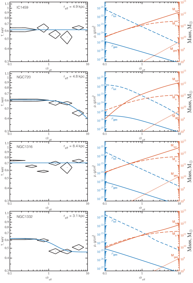
Figure 6: Left: Interstellar gas temperature versus radius (in units of the effective radius) for the galaxies from Table 2. The diamonds denote the observed temperature with errors; the solid lines indicate the fit from Eqs. (4)–(6). Right: The left vertical axes correspond to the gas densities ($\rho_{\rm gas}$, the solid line) and the total mass ($\rho_{\rm tot}$, the dashed line) found from Eqs. (1) and (7). The right vertical axes correspond to the profiles of the total mass ($M_{\rm tot}$ , the solid line), the gas mass ($M_{\rm gas}$, the dotted line), and the best fit to the stellar component ($M_{\rm s}$, the dash line).

where $k_{b}$ and $G$ are the Boltzmann and gravitational constants, respectively; $\mu$ is the mean molecular weight, $\mu\approx 0.62$ for solar element abundances; and $n=(1+X)n_{e}$ is the particle number density. The derived temperature and density profiles of the ISM as well as the mass profiles are presented below in Fig. 6.

4 Diffusion calculations

Depending on the strength and topology of the magnetic field as well as the MHD turbulence characteristics, the transport processes in the ISM can be significantly suppressed by the magnetic fields. A simple approach is to introduce a constant suppression factor (in the context of diffusion in the ICM, see Peng & Nagai, 2009a): $S_{B}\equiv\kappa/\kappa_{sp}\leqslant 1$, where $\kappa_{sp}$ is the Spitzer thermal conductivity of a non-magnetized plasma (Spitzer, 1962). The current theoretical constrains on the suppression magnitude is provided by numerical simulations only for the ICM plasma in galaxy clusters. In this case the global thermal conductivity is expected to be moderately suppressed in a tangled magnetic field of the ICM plasma: $S_{B}\sim 0.1$–$0.2$ (Chandran & Cowley, 1998; Narayan & Medvedev, 2001; Chandran & Maron, 2004). Besides that, the weakly collisional magnetized plasma of the ICM is subject to a wide variety of instabilities, such as the firehose and mirror instabilities, which can suppress transport efficiency by another factor of 5–10 (Riquelme et al., 2016; Komarov et al., 2016). However the collision mean free path and other physical properties of the ISM can be considerably different from that of the ICM, therefore, the role of the above-mentioned instabilities remains unclear and requires further numerical simulations. In this paper the ISM plasma is assumed to be non-magnetized ($S_{B}=1$), i.e., we estimate the maximum possible effect of diffusion.

To calculate the element diffusion in the ISM, we use the same numerical scheme as developed by Shtykovskiy & Gilfanov (2010) to model the diffusion in the ICM. We consider the Burgers’ flow equations for the mass, momentum, and energy conservation. Under the assumption of hydrostatic equilibrium, spherical symmetry and the same temperature for all gas species the Burgers’ equations are (Burgers, 1969; Thoul et al., 1994)

$$\frac{\partial{n_{s}}}{\partial{t}}+\frac{1}{r^{2}}\frac{\partial}{\partial{r}}[r^{2}n_{s}\,(w_{s}+u)]=0,$$ (8)

$$\frac{d(n_{s}k_{B}T)}{dr}+n_{s}m_{s}g-n_{s}Z_{s}eE=\sum_{t\neq s}K_{st}[(w_{t}-w_{s})+\\ +0.6(x_{st}r_{s}-y_{st}r_{t})],$$ (9)

$$\frac{5}{2}n_{s}k_{B}\frac{dT}{dr}=\sum_{t\neq s}K_{st}\{\frac{3}{2}x_{st}(w_{s}-w_{t})-\\ -y_{st}[1.6x_{st}(r_{s}+r_{t})+Y_{st}r_{s}-4.3x_{st}r_{t}]\}-0.8K_{ss}r_{s},$$ (10)

where $g=[GM(r)/r^{2}]$ is the gravitational acceleration modulus, $E$ is the radial induced electric field, $m_{s}$ is the mass of particles of species $s$, $\mu_{st}=m_{s}m_{t}/(m_{s}+m_{t})$, $x_{st}=\mu_{st}/m_{s}$, $y_{st}=\mu_{st}/m_{t}$ and $Y_{st}=3y_{st}+1.3x_{st}m_{t}/m_{s}$. The numerical coefficients in these equations correspond to Coulomb potential with a long-range cut-off at the Debye length. The gas viscosity in Eqs. 9–10 is assumed to be negligible.

The friction coefficient $K_{s,t}$ between particles of species $s$ and $t$ for a Coulomb interaction potential is defined by the expression (Chapman & Cowling, 1991):

$$K_{st}=(2/3)\mu_{st}(2k_{B}T/\mu_{st})^{1/2}n_{s}n_{t}\sigma_{st},$$ (11)

where the transport cross-section is:

$$\sigma_{st}=2\sqrt{\pi}e^{4}Z_{s}^{2}Z_{t}^{2}(k_{B}T)^{-2}\ln\Lambda_{st}.$$ (12)

Since the ISM gas is considerably denser and colder than the ICM, the Coulomb logarithm, $\ln\Lambda_{st}$, can be considerably smaller than 40 (the typical value for the ICM conditions). Nevertheless, the condition $\Lambda_{st}\gg 1$ (ideal plasma) is always fulfilled for the ISM plasma. Therefore, we use the approximate formulas by Huba (2009) for a Coulomb potential with shielding at the Debye length. Denote the gas temperature in eV by $T_{{\rm eV}}$ and the plasma electron component by the subscript $e$. For the ion–ion interaction

$$\ln\Lambda_{st}=23-\ln\left[\frac{Z_{s}Z_{t}}{T_{{\rm eV}}^{3/2}}(n_{s}Z_{s}^{2}+n_{t}Z_{t}^{2})^{1/2}\right].$$ (13)

For the electron–electron interaction

$$\ln\Lambda_{ee}=23.5-\ln n_{e}^{1/2}T_{{\rm eV}}^{-5/4}-[10^{-5}+(\ln T_{{\rm eV}}-2)^{2}/16]^{1/2}.$$ (14)

For the ion–electron interaction, if $T_{{\rm eV}}m_{e}/m_{s}<T_{{\rm eV}}<10Z_{s}^{2}\,{{\rm eV}}$,

$$\ln\Lambda_{se}=23-\ln n_{e}^{1/2}Z_{s}T_{{\rm eV}}^{-3/2},$$ (15)

and for $T_{{\rm eV}}m_{e}/m_{s}<10Z_{s}^{2}\,{{\rm eV}}<T_{{\rm eV}}$:

$$\ln\Lambda_{se}=24-\ln n_{e}^{1/2}T_{\rm eV}^{-1}.$$ (16)

For all interactions $\ln\Lambda_{st}=\ln\Lambda_{ts}$. In the ranges of temperatures and densities of interest to us the Coulomb logarithm lies within the range 30–37. When passing from Eq. (15) to (16), a discontinuity emerges in the derivative of the diffusion velocity. To prevent the ensuing numerical instability of our calculations, we used Eq. (15) for ions with a nuclear charge $>+8$ and Eq. (16) for ions with a smaller charge. The values of the Coulomb logarithm obtained in this way lie within the accuracy of the approximate formulas, 10% (Huba, 2009).

The thermal diffusion occurs due to the interference between Eq. 9 and 10 via the quantities $r_{s}$, which are the so-called residual heat flow velocities defined as the local heat flow transported by particles of species $s$, divided by the partial pressure $p_{s}$ (Burgers, 1969). A phenomenological explanation of the thermal diffusion can be found, e.g., in Monchick & Mason (1967). For the the Coulomb cross-section given by Eq.12, the thermal diffusion tends to move the more highly charged and more massive particles up the temperature gradient. Note that even in the absence of a temperature gradient the total local heat flow $Q=\sum r_{s}n_{s}k_{b}T$, even if small, is nonzero (Chuzhoy & Loeb, 2004). As in the case of galaxy clusters, we deemed the temperature profile to be constant in time ($T(t)={\rm const}$) during the entire calculations by assuming an equilibrium between the heating and cooling of the ISM.

The diffusion velocities obey the mass and charge (the absence of a current) conservation laws that should be added to the set of equations (9)–(10):

$$\sum\rho_{i}w_{i}=0,$$ (17)

$$\sum Z_{i}n_{i}w_{i}=0.$$ (18)

As a result of sedimentation, the mean molecular weight of particles in the galactic central region, $\mu=\sum m_{i}n_{i}/m_{p}n$, increases. This causes the total local gas pressure to decrease and the hydrostatic equilibrium to be upset. However, the system rapidly returns to an equilibrium state due to the net mass flow into the galactic central region:

$$\frac{du}{dt}=-\frac{\nabla p}{\rho}-g.$$ (19)

Since the characteristic diffusion time scale is always larger than the characteristic hydrodynamic time by many orders of magnitude, Eqs. (9)–(10) remain applicable, because the inertial terms ($\sim du_{s}/dt$) in Eqs. (9)–(10) make a negligible contribution. Equations (8)–(19) completely define the diffusion velocities $w_{s}$, the quantities $r_{s}$, the low gas flow velocity $u$, and the induced electric field strength $E$.

4.1 Description of the Model

To solve the set of equations (8)–(19), we use a homogeneous spatial grid covering the region from 0 to $10\,r_{\rm eff}$ (22–85 kpc) for each galaxy. The spatial grid step is 7–28 pc. The time step is specified so as to ensure the numerical stability of the scheme, $dt=2.5\times 10^{3}$ yr. We limit the diffusion calculation by 2 Gyr.

As an outer boundary condition for the continuity equation, the particle number density was specified to be equal to the initial one at the outer boundary of the computational domain. This boundary condition qualitatively corresponds to a galaxy placed in an infinite gas reservoir with a fixed density. To calculate the velocities (Eqs. (9), (10), (19)) at the outer boundary, we used one-sided derivatives. At $r=0$ the number density was calculated by expanding Eq. (8) near zero (see Shtykovskiy & Gilfanov, 2010). The velocities at $r=0$ were assumed to be zero.

The derived analytical expressions (Eq. 2–6) for the gas temperature and density were extrapolated to $10\,r_{\rm eff}$. This reduces the influence of outer boundary conditions on the results of our calculations for the region of galaxies under study ($r\leq 8\,r_{\rm eff}$). We tested our solution by replacing the outer boundary condition with an “opaque wall” (all velocities are zero). For the galaxy with the strongest diffusion at large radii, NGC 4636, this replacement leads to significant changes only for the region $r>9\,r_{\rm eff}$ ($\sim 10$% in the change of He to H). For the mass of any element within $r<8\,r_{\rm eff}$ the difference in 2 Gyr does not exceed 8%; the difference within $r<4\,r_{\rm eff}$ is less than 4%. The net mass flow (Eq. (19)) causes the gas mass in the galaxy to increase by 5% in 2 Gyr of diffusion. For the remaining galaxies the differences turn out to be even smaller.

We also checked that the Coulomb mean free path (Eq. 12) is always much smaller than the size of the computational region. In the temperature and density ranges under consideration the mean free path lies within the range $10^{-9}<\lambda_{C}<0.1$ kpc.

The abundances of all elements at the initial time of our simulations were assumed to be solar (Lodders, 2003) and identical at all radii. Although the heavy-element abundances in the interstellar gas of early-type galaxies can be considerably lower than the solar ones (Su & Irwin, 2013), this affects weakly the diffusion calculations, because the heavy elements are a small admixture in the H–He plasma.

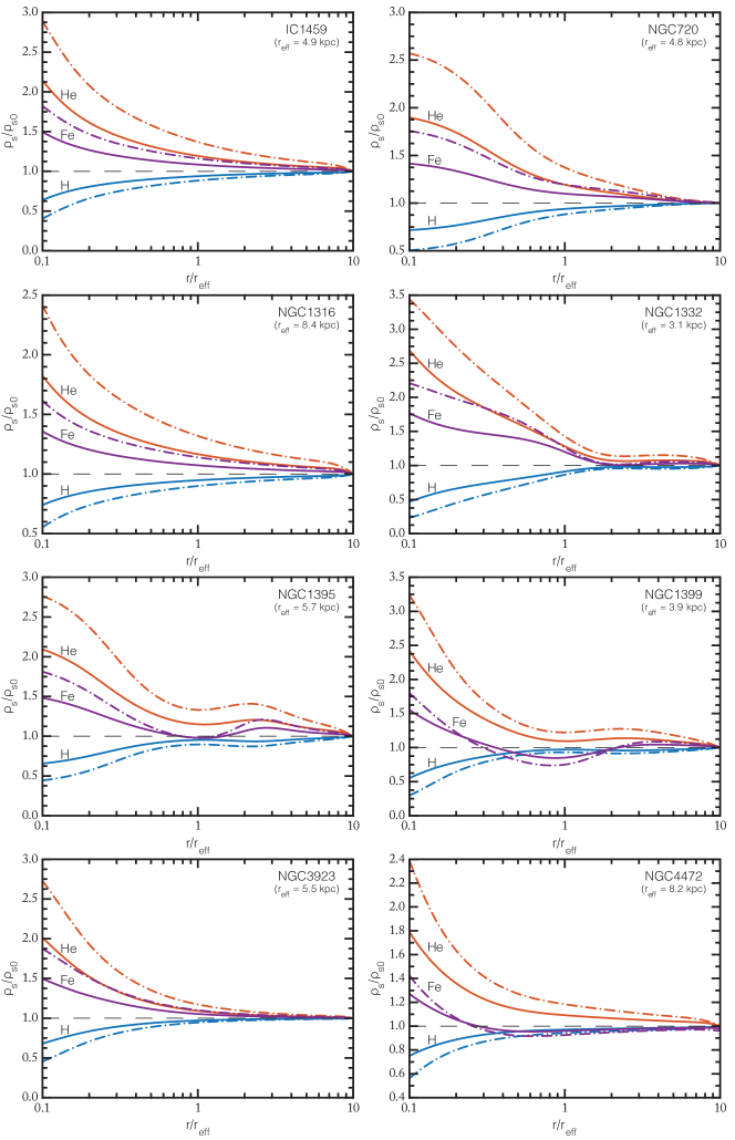
Figure 1: Hydrogen (blue lines), He III (red lines), and Fe XXII (purple lines) density distributions as a function of radius (in units of the effective radius) after 1 (solid lines) and 2 (dash-dotted lines) Gyr of diffusion. The results of our calculations are presented for the galaxies from Table 2.

5 Results

5.1 The Spatial Distribution of Elements

The spatial distributions of elements after 1 and 2 Gyr of diffusion are presented in Fig. 1. The results for hydrogen (blue lines), helium (red lines), and Fe XXII (purple lines) are shown. Fe XXII was chosen to demonstrate the diffusion of heavy ions; a slight change in the ionization fraction ($\pm 2$) affects weakly the result (within 1%). For all of the chosen galaxies diffusion leads to an increase in the abundances of elements heavier than hydrogen within $r_{\rm eff}$. The greatest effect is expected for helium. A strong dependence of the element abundance profile on temperature gradient is seen in Fig. 6. The temperature gradient exerts the greatest influence on the iron diffusion due to the dependence of thermal diffusion on nuclear charge. Thus, accurate measurements of the heavy-element abundances in the ISM could provide additional information both about the gas temperature profile and about the transport efficiency in the gas (or the magnetic field strength). However, this method will probably be difficult to apply in practice, because it is necessary to take into account the enrichment of the interstellar medium with heavy elements from stellar winds and during supernova explosions as well as the turbulent mixing and resonant scattering in metal lines (Gilfanov & Syunyaev, 1984; Zhuravleva et al., 2010).

5.2 Change in the Mass Fraction of Elements

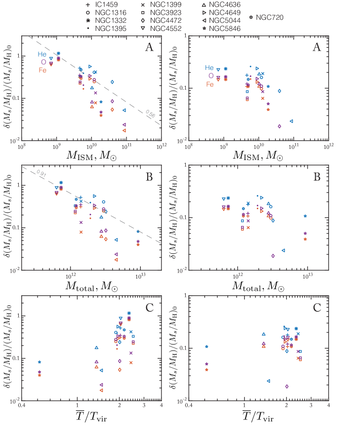
Figure 2: Relative change in the He III (blue symbols), O VIII (purple symbols), and Fe XXII (red symbols) mass divided by the hydrogen mass within 1 (left panels A, B, and C) and 4 (right panels A, B, and C) effective radii after 1 Gyr of diffusion as a function of the interstellar gas mass within $10\,r_{\rm eff}$ (panel A), the total mass within $10\,r_{\rm eff}$ (B), and the mean temperature $\overline{T}$ (determined from Eq. 4, panel C) divided by $T_{\rm vir}=\gamma\mu m_{p}GM/(3\times 10\,r_{\rm eff})$ (for more details, see the text). The gray dashed line indicates the fit to the helium change by a power law with its index specified near the line.

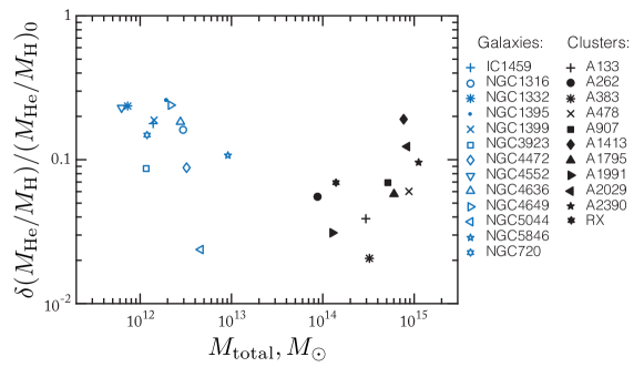
Figure 3: Relative increase in the helium mass divided by the hydrogen mass for the galaxies of our sample and clusters from Vikhlinin et al. (2006) as a function of the total mass after 1 Gyr of diffusion. We calculated the hydrogen and helium mass for the galaxies within $4\,r_{\rm eff}$ and the total mass within $10\,r_{\rm eff}$. For the galaxy clusters the corresponding sizes were taken to be $0.08\,r_{\rm 500}$ and $r_{\rm 500}$ (see the text). “RX” denotes the “X-ray superbright elliptical galaxy” RX J1159$+$5531.

We see that for most galaxies (NGC 1332,NGC 1395, NGC 1399, NGC 4472, NGC 4636, NGC 5044, NGC 5846) the effect of thermal diffusion dominates over the gravitational sedimentation of iron in the places where the temperature gradient is largest. All these galaxies, except NGC 1395, are at the group center (environment type 2, see Table 2). The element sedimentation profile in the galaxy NGC 4636, where helium (and to a lesser degree iron) is accumulated in the entire observed region ($r_{\rm eff}$–$8\,r_{\rm eff}$), is of greatest interest. In the remaining cases, the greatest increase in element abundances occurs in a small central region, $r<0.3\ r_{\rm eff}\sim 0.7$–$2.5$ kpc. The huge effect of diffusion at $r\sim 5$–$6\,r_{\rm eff}$ for the galaxy NGC 5846 is associated with a sharp drop in density at $r>4\,r_{\rm eff}$ and simultaneously a high gas temperature. For comparison, diffusion in NGC 4552, on the whole, affects weakly the element abundances, despite the fact that the gas density at large radii in NGC 4552 and NGC 5846 is of the same order of magnitude.

The right and left panels in Fig. 2 show the change in the mass contained in different elements in the galaxies being studied after 1 Gyr of diffusion within $r_{\rm eff}$ and $4\,r_{\rm eff}$, respectively. Apart from the iron diffusion, we calculate the diffusion of the main groups of heavy elements: O VIII and Si XIII (the result for Si XIII is not shown, because the points are close to O VIII, but listed in Table 3). The results are shown in the form of dependences of the relative change in the mass of an element divided by the hydrogen mass ($\frac{M_{s}}{M_{{\rm H}}}/(\frac{M_{s}}{M_{{\rm H}}})_{t=0}-1$) on (A) the ISM gas mass within $10\,r_{\rm eff}$ (i.e., the total volume of the computational domain) found by integrating the gas density, (B) the total mass within $10\,r_{\rm eff}$ derived from the hydrostatic equilibrium condition, and (C) the ratio $\overline{T}/T_{\rm vir}$, where $\overline{T}$ is the mean gas temperature obtained by fitting the measured temperature profile by Eq. (4), and $T_{\rm vir}=\gamma\mu m_{p}GM/(3\times 10\,r_{\rm eff})$ (where $\mu=0.62$, $\gamma=1.2$) is the “virial” temperature corresponding to the galactic gravitational potential (Makino et al., 1998). The results of our calculations are also presented in Table 3.

We see that the integrated effect of diffusion grows with decreasing gas mass and total mass of the galaxy. This is partly related to an increase in the ratio $\overline{T}/T_{{\rm vir}}$ for such objects (right panels). The decrease of the gas fraction, $f_{b}$, in lower-mass galaxies serves as an additional factor, with the diffusion velocity being $\sim f_{b}^{-1}$ (Peng & Nagai, 2009a). The increase in the concentration of heavy elements, on the whole, follows the change in the helium abundance.

5.3 Comparison with the Diffusion in Galaxy Clusters

It is interesting to compare the calculated change in the abundances of elements due to diffusion in early-type galaxies with the expected result of diffusion in galaxy clusters; the sample of clusters from Vikhlinin et al. (2006) can be used in this case. We use the results from Shtykovskiy & Gilfanov (2010) and Medvedev et al. (2014) for the clusters A262 and A2029, respectively, and calculate the diffusion in a similar way for the remaining clusters using the best-fit formulas for the temperature and density from Vikhlinin et al. (2006) by extrapolating them to the cluster center. During our calculations the ICM gas is assumed to be in hydrostatic equilibrium in the gravitational potential of a dark matter cluster halo with an NFW density profile (Navarro et al., 1997). For a more detailed description, see Shtykovskiy & Gilfanov (2010).

To compare the results of diffusion in clusters and galaxies, it is necessary to choose a spatial scale within which the integrated effect could be calculated. It is convenient to choose the radius $r_{\rm 500}$ as such a scale. Unfortunately, the ISM region accessible to measurements turns out to be smaller than $r_{\rm 500}$ by an order of magnitude. Therefore, we can give only a rough estimate of this radius for the galaxies of our sample: $r_{e}\sim 0.02\,r_{\rm 500}$ (see Section 2).

Figure 3 compares the relative increase of the helium mass divided by the hydrogen mass for the galaxies of our sample and clusters from Vikhlinin et al. (2006) as a function of the total mass after 1 Gyr of diffusion. In the case of galaxies, we determine the helium and hydrogen mass within $4\,r_{\rm eff}$ and the total mass within $10\,r_{\rm eff}$. For the clusters we calculate the helium and hydrogen mass within $0.08\,r_{\rm 500}$ and the total mass within $r_{\rm 500}$; $r_{\rm 500}$ is taken from Vikhlinin et al. (2006). The sedimentation amplitude in early-type galaxies is seen to be comparable to that in galaxy clusters. Interestingly, in the case of clusters the effect is enhanced for more massive clusters, while in the case of galaxies an inverse dependence is observed. For the clusters this result is a consequence of the increase in the temperature of the ICM with increasing cluster mass. We checked that a change in the radius within which the effect is calculated for galaxy clusters ($0.08\,r_{\rm 500}$) does not affect the general dependence of the sedimentation amplitude on cluster mass.

5.4 Helium Sedimentation

A significant increase of the helium abundance in the entire ISM volume under consideration, with the greatest value in the central region $<1\,r_{\rm eff}$, is expected from the results of our calculations. The largest increase in the helium mass relative to hydrogen is expected at the center of NGC 1332, 115% in 1 Gyr (by more than a factor of 2). This is one of the least massive galaxies in our sample. For the lowest-mass galaxy from the sample, NGC 4552, the expected increase in the helium abundance within $r_{\rm eff}$ is 88%. A maximum increase in helium within $4\,r_{\rm eff}$ is expected for the large galaxy NGC 1395, 25.8%, while a maximum increase in the total helium mass (within $10\,r_{\rm eff}$) is expected for the galaxy NGC 5846, 26%.

The deviation of the helium abundance from its solar value turns out to be important in analyzing the X-ray observations (Drake, 1998; Ettori & Fabian, 2006; Markevitch, 2007; Peng & Nagai, 2009a; Medvedev et al., 2014). Since the helium abundance cannot be directly estimated from X-ray spectroscopy, the helium abundance is commonly assumed to be solar when analyzing the spectra. This assumption leads to a biased estimate of the quantities derived from X-ray spectroscopy: the gas temperature, density, and heavy-element abundances. To find the amplitude of these biases, we perform the following test (see Medvedev et al., 2014). Using the vvAPEC model (AtomDB/APEC, version 3.0.6, Foster et al. 2012) in the XSPEC software (heasoft v6.19, Arnaud 1996), we generate a set of thermal spectra for an optically thin hot plasma in wide ranges of temperatures ($0.1<T^{\rm tr}<8$) and helium abundances ($0<x^{\rm tr}<5$, in solar units). The abundances of the remaining elements are assumed to be solar (Lodders, 2003). Next, for each such spectrum we model the spectrum that could be measured with the Chandra ACIS-S camera (the data on the instrumental response are taken for ACIS Cycle 18) by means of the fakeit command. We assume that the data could be obtained with a long exposure; therefore, no random noise is added to the model spectra. As a result, the derived spectra are fitted in the energy range 0.5–10 keV by the APEC model, with the helium abundance having been fixed at its solar value.

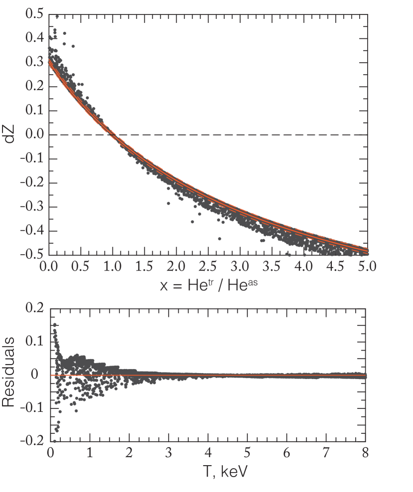
Figure 4: Error in the metal abundance $dZ=Z^{{\rm tr}}/Z^{{\rm fit}}-1$ under the erroneous assumption about the helium abundance $x={\rm He}^{{\rm tr}}/{\rm He}^{{\rm as}}$. The black dots correspond to the result of our numerical test (see the text), the solid line indicates the fit by Eq. (20). The red dash-dotted line indicates the region that contains 95% of the dots. The lower panel shows the residuals of our numerical test and the fit as a function of gas temperature.

In the temperature range under consideration an optically thin H–He plasma radiates mostly by bremsstrahlung. In that case, the integrated specific energy release depends on the square of the nuclear charge of the ion interacting with the electron. This leads to a change of the continuum level in the plasma spectrum when varying the helium abundance (${\rm He}^{{\rm tr}}$). Therefore, the heavy-element abundances ($Z^{{\rm fit}}$) found by fitting this spectrum by a model with a solar helium abundance (${\rm He}^{{\rm as}}$) will be biased relative to those specified in the model ($Z^{{\rm tr}}$). The shape of the bremsstrahlung spectrum also depends on the nuclear charge, but to a lesser degree (the charge dependence of the Gaunt factor; see, e.g., Rybicki & Lightman 1979). This effect leads to a biased estimate of the gas temperature ($T^{{\rm fit}}$).

The results of the test described above for $2\times 10^{4}$ realizations are presented in Fig. 4. There is a significant bias of the heavy-element abundances that can be described by a simple approximate formula:

$$dZ=(1-x)/(3.28+x),$$ (20)

where $x={\rm He}^{{\rm tr}}/{\rm He}^{{\rm as}}$ is the deviation of the helium abundance from the solar one and $dZ=Z^{{\rm fit}}/Z^{{\rm tr}}-1$ is the error in the metal abundance. The visible “step” on the panel with residuals is equal to the step in the temperatures for which the spectroscopic AtomDB data were computed and is associated with the XSPEC interpolation for intermediate temperatures. However, this effect does not affect the main trend of the residual. We made sure of this by applying the vMEKAL and MEKAL models (Kaastra, 1992) in a similar way by calculating the thermal spectrum for each temperature (without using any interpolation). The result obtained is analogous to the APEC model. We see that the error in the metal abundance increases for a temperature $T^{{\rm tr}}<4$ keV. Thus, at $T^{{\rm tr}}\sim 0.1$ keV determining the heavy element abundances by fitting the thermal spectrum at energies $>0.5$ keV can lead to an uncertain result that will depend strongly on the assumed helium abundance. The associated error in the temperature determination turns out to be insignificant, $dT=T^{{\rm fit}}/T^{{\rm tr}}-1<0.03$, with the biased estimate of the metal abundance contributing to this error.

A variation of the helium abundance ${\rm He}^{{\rm tr}}$ also leads to a change in the ratio of the determined and specified normalization quantities: $\eta\equiv\frac{N^{{\rm fit}}}{N^{{\rm tr}}}\sim\frac{n^{{\rm fit}}_{H}n^{{\rm fit}}_{e}}{n^{{\rm tr}}_{H}n^{{\rm tr}}_{e}}$. However, $\eta$ gives no direct information about the error in the gas density. Fixing the solar hydrogen abundance in the vvAPEC model and varying the helium abundance implies changing the total density in the model of a plasma. Therefore, the change in $\eta$ when fitting this spectrum by the APEC model reflects mainly the actual change of the density in the plasma model.

5.5 The Impact of Thermal Diffusion

To demonstrate an important role of the thermal diffusion, we perform additional calculations by artificially removing the terms proportional to $r_{s}$ from Eq. (9). In that case, Eq. 10 is not used. These calculations were performed for NGC 1399 with the highest mean temperature, $\overline{T}=0.93$ keV, and NGC 3923 with the lowest mean temperature, $\overline{T}=0.56$ keV.

Figure 5 shows the ratio of the helium (red lines) and iron (black lines) abundances derived with and without thermal diffusion (the element abundance is defined as $n_{s}/n_{{\rm H}}$). We show the result for NGC 1399 for 1 and 2 Gyr and for NGC 3923 for 1 Gyr. We see that thermal diffusion changes significantly the element abundance profile and the amplitude of the effect. Thermal diffusion exerts the greatest influence on ions with a large nuclear charge. In addition, thermal diffusion slows down the sedimentation of elements heavier than hydrogen for NGC 1399, whose temperature profile has a positive gradient. For NGC 3923 the reverse is true: thermal diffusion accelerates the sedimentation of elements, because the temperature profile has a negative gradient. The same is also characteristic of all low-mass galaxies, where the temperature gradient is negative.

Figure 5: Spatial distribution of the He III (red lines) and Fe XXII (black lines) abundances calculated with thermal diffusion divided by the corresponding distribution found without thermal diffusion. The results are shown for 1 (solid lines) and 2 (long dashed lines) Gyr for NGC 1399 and 1 Gyr (dash-dotted lines) for NGC 3923.

6 Conclusions

We calculated the diffusion of elements in the interstellar medium (ISM) for 13  early-type galaxies. To estimate the maximum effect of diffusion, we considered the full set of Burgers’ equations in the approximation of a non-magnetized ISM plasma using observational data for the gas density and temperature. Our calculations showed that a significant gravitational sedimentation of helium and other heavy elements is possible. For X-ray-bright galaxies with a rising radial temperature profile the average relative increase of the helium mass is 23% within $1\,r_{\rm eff}$ in 1 Gyr. For less massive galaxies with a flat or declining radial temperature profiles the corresponding increase in helium is 60%. The effect of thermal diffusion accelerates significantly the sedimentation of elements for galaxies of this type, while for cool-core galaxies thermal diffusion leads to a reduction in sedimentation.

We compared our results with the gravitational helium sedimentation amplitude in cool-core galaxy clusters. It turned out that the helium abundance in the ISM could change equally significantly as in the ICM plasma. This occurs despite the fact that the temperature of the ISM is considerably lower than the ICM temperature. The strong effect of diffusion in the ISM is associated with a lower gas mass fraction and a complex mass–temperatures relation for early-type galaxies.

Helium sedimentation may be partially responsible for the reduced heavy element abundances determined from X-ray spectroscopy. A two-fold increase in the helium abundance relative to the solar value leads to an underestimation of the metal abundance by 20%.

An interstellar medium with an enhanced helium abundance can affect the evolution of the galactic stellar population. Whereas most early-type galaxies contain mainly an old stellar population, observational data demonstrate that the star formation process still takes place in some of such objects (see, e.g., O’Dea et al., 2008). In particular, in large elliptical galaxies at the center of cool-core clusters the star formation rate can reach dozens of$M_{\sun}\,\mbox{year}^{-1}$ (O’Dea et al., 2008). Thus, as a result of sedimentation, the cooling ISM gas can form helium enriched stars that leave the main sequence more rapidly. Therefore, hot stars can fall on the horizontal branch of the Hertzsprung-Russell diagram more effectively. Such stars are brighter in the ultraviolet, which can be responsible for the ultraviolet upturn in early-type galaxies (Dorman et al., 1995; Peng & Nagai, 2009b).

The Chandra  and XMM-Newton  X-ray observatories have already observed dozens of early-type galaxies. This allows the physical processes in the interstellar gas of galaxies to be studied in detail. Adding the diffusion of elements to the simulations of such objects can help in forming a clear understanding of their observational properties.

Table 3: Change in the mass fraction of elements in the interstellar gas within $1\,r_{\rm eff}$, $4\,r_{\rm eff}$ and $10\,r_{\rm eff}$ after 1 (2) Gyr of diffusion.The change in the mass fraction of an element ($s=$ He III, O VIII, Si XIII, Fe XXII), divided by the hydrogen mass: $(\frac{M_{s}}{M_{{\rm H}}}/\left(\frac{M_{s}}{M_{{\rm H}}}\right)_{t=0}-1)\times 100$, where the mass is calculated within $1\,r_{\rm eff}$, $4\,r_{\rm eff}$, and $10\,r_{\rm eff}$. The values for 2 and 1 Gyr of diffusion are given in and without parentheses, respectively.

Galaxy	He III/H	O VIII/H	Si XIII/H	Fe XXII/H	He III/H	O VIII/H	Si XIII/H	Fe XXII/H	He III/H
	$<1\,r_{\rm eff}$				$<4\,r_{\rm eff}$				$<10\,r_{\rm eff}$
IC1459	51.4 (110.5)	35.1 (75.3)	31.4 (67.5)	29.5 (63.5)	17.6 (36.4)	12.0 (24.8)	10.8 (22.2)	10.1 (20.9)	8.1 (15.9)
NGC720	46.8 (101.9)	32.8 (71.7)	29.7 (64.9)	28.0 (61.3)	14.8 (30.1)	11.6 (23.7)	10.8 (22.1)	10.4 (21.2)	4.7 (9.4)
NGC1316	40.6 (85.8)	27.7 (58.4)	24.8 (52.4)	23.3 (49.2)	16.0 (33.0)	10.9 (22.5)	9.8 (20.2)	9.2 (18.9)	8.1 (15.8)
NGC1332	114.5 (243.2)	88.5 (188.5)	82.1 (175.3)	78.6 (168.1)	23.4 (48.7)	16.4 (33.9)	14.8 (30.6)	14.0 (28.9)	11.1 (21.7)
NGC1395	38.8 (84.0)	20.5 (43.3)	16.7 (35.6)	14.8 (31.7)	25.8 (54.7)	17.0 (36.3)	15.0 (32.1)	13.9 (29.9)	12.0 (23.4)
NGC1399	41.8 (90.0)	13.4 (28.1)	7.8 (17.3)	5.1 (12.1)	18.8 (39.6)	8.7 (18.6)	6.4 (14.0)	5.3 (11.7)	8.6 (16.5)
NGC3923	32.6 (67.2)	24.5 (50.6)	22.6 (46.7)	21.6 (44.7)	8.6 (17.3)	6.5 (13.1)	6.0 (12.1)	5.8 (11.6)	3.5 (7.0)
NGC4472	23.9 (50.2)	8.6 (18.1)	5.4 (11.7)	3.8 (8.6)	8.7 (17.9)	1.9 (4.0)	0.4 (1.1)	-0.3 (-0.4)	4.3 (8.2)
NGC4552	88.0 (181.3)	68.7 (139.7)	64.0 (130.1)	61.6 (125.0)	22.7 (47.3)	16.2 (33.4)	14.7 (30.4)	13.9 (28.8)	14.1 (27.6)
NGC4636	17.5 (38.4)	8.1 (18.5)	6.2 (14.6)	5.2 (12.6)	18.3 (38.3)	12.1 (25.4)	10.8 (22.6)	10.0 (21.1)	10.7 (21.0)
NGC4649	55.7 (123.1)	33.7 (74.2)	29.0 (64.3)	26.6 (59.2)	23.7 (50.0)	15.1 (32.0)	13.2 (28.1)	12.2 (26.0)	11.3 (21.9)
NGC5044	5.2 (10.4)	2.4 (4.7)	1.7 (3.5)	1.4 (2.8)	2.3 (4.8)	0.1 (0.3)	-0.3 (-0.6)	-0.6 (-1.1)	3.5 (6.7)
NGC5846	8.1 (15.3)	4.7 (8.8)	4.0 (7.4)	3.6 (6.6)	10.7 (26.4)	5.0 (12.8)	3.9 (10.4)	3.3 (9.2)	25.9 (49.0)

References

- Anders & Grevesse (1989) Anders E., Grevesse N., 1989, Geochim. Cosmochim. Acta, 53, 197
- Arnaud (1996) Arnaud K. A., 1996, in Jacoby G. H., Barnes J., eds, Astronomical Society of the Pacific Conference Series Vol. 101, Astronomical Data Analysis Software and Systems V. p. 17, http://adsabs.harvard.edu/abs/1996ASPC..101...17A
- Boroson et al. (2011) Boroson B., Kim D.-W., Fabbiano G., 2011, ApJ, 729, 12
- Buote (2000) Buote D. A., 2000, ApJ, 539, 172
- Burgers (1969) Burgers J. M., 1969, Flow Equations for Composite Gases. http://adsabs.harvard.edu/abs/1969fecg.book.....B
- Chandran & Cowley (1998) Chandran B. D. G., Cowley S. C., 1998, Physical Review Letters, 80, 3077
- Chandran & Maron (2004) Chandran B. D. G., Maron J. L., 2004, ApJ, 602, 170
- Chapman & Cowling (1991) Chapman S., Cowling T. G., 1991, The Mathematical Theory of Non-uniform Gases. http://adsabs.harvard.edu/abs/1991mtnu.book.....C
- Chuzhoy & Loeb (2004) Chuzhoy L., Loeb A., 2004, MNRAS, 349, L13
- Ciotti et al. (1991) Ciotti L., D’Ercole A., Pellegrini S., Renzini A., 1991, ApJ, 376, 380
- Dorman et al. (1995) Dorman B., O’Connell R. W., Rood R. T., 1995, ApJ, 442, 105
- Drake (1998) Drake J. J., 1998, ApJ, 496, L33
- Ettori & Fabian (2006) Ettori S., Fabian A. C., 2006, MNRAS, 369, L42
- Faber et al. (1989) Faber S. M., Wegner G., Burstein D., Davies R. L., Dressler A., Lynden-Bell D., Terlevich R. J., 1989, ApJS, 71, 173
- Fabian & Pringle (1977) Fabian A. C., Pringle J. E., 1977, MNRAS, 181, 5P
- Foster et al. (2012) Foster A. R., Ji L., Smith R. K., Brickhouse N. S., 2012, ApJ, 756, 128
- Fukazawa et al. (2006) Fukazawa Y., Botoya-Nonesa J. G., Pu J., Ohto A., Kawano N., 2006, ApJ, 636, 698
- Gilfanov & Syunyaev (1984) Gilfanov M. R., Syunyaev R. A., 1984, Soviet Astronomy Letters, 10, 137
- Huba (2009) Huba J., 2009, Technical report, NRL Plasma Formulary 2009. NAVAL RESEARCH LAB WASHINGTON DC BEAM PHYSICS BRANCH
- Humphrey et al. (2004) Humphrey P. J., Buote D. A., Canizares C. R., 2004, ApJ, 617, 1047
- Humphrey et al. (2006) Humphrey P. J., Buote D. A., Gastaldello F., Zappacosta L., Bullock J. S., Brighenti F., Mathews W. G., 2006, ApJ, 646, 899
- Humphrey et al. (2011) Humphrey P. J., Buote D. A., Canizares C. R., Fabian A. C., Miller J. M., 2011, ApJ, 729, 53
- Jones et al. (2002) Jones C., Forman W., Vikhlinin A., Markevitch M., David L., Warmflash A., Murray S., Nulsen P. E. J., 2002, ApJ, 567, L115
- Kaastra (1992) Kaastra J., 1992, An X-ray spectral code for optically thin plasmas
- Kim & Fabbiano (2003) Kim D.-W., Fabbiano G., 2003, ApJ, 586, 826
- Komarov et al. (2016) Komarov S. V., Churazov E. M., Kunz M. W., Schekochihin A. A., 2016, MNRAS, 460, 467
- Lodders (2003) Lodders K., 2003, ApJ, 591, 1220
- Makino et al. (1998) Makino N., Sasaki S., Suto Y., 1998, ApJ, 497, 555
- Markevitch (2007) Markevitch M., 2007, preprint (arXiv:0705.3289)
- Mathiesen & Evrard (2001) Mathiesen B. F., Evrard A. E., 2001, ApJ, 546, 100
- Medvedev et al. (2014) Medvedev P., Gilfanov M., Sazonov S., Shtykovskiy P., 2014, MNRAS, 440, 2464
- Medvedev et al. (2016) Medvedev P., Sazonov S., Gilfanov M., 2016, MNRAS, 459, 431
- Monchick & Mason (1967) Monchick L., Mason E. A., 1967, Physics of Fluids, 10, 1377
- Nagino & Matsushita (2009) Nagino R., Matsushita K., 2009, A&A, 501, 157
- Narayan & Medvedev (2001) Narayan R., Medvedev M. V., 2001, ApJ, 562, L129
- Navarro et al. (1997) Navarro J. F., Frenk C. S., White S. D. M., 1997, ApJ, 490, 493
- O’Dea et al. (2008) O’Dea C. P., et al., 2008, ApJ, 681, 1035
- O’Sullivan et al. (2003) O’Sullivan E., Ponman T. J., Collins R. S., 2003, MNRAS, 340, 1375
- Pellegrini (2011) Pellegrini S., 2011, ApJ, 738, 57
- Peng & Nagai (2009a) Peng F., Nagai D., 2009a, ApJ, 693, 839
- Peng & Nagai (2009b) Peng F., Nagai D., 2009b, ApJ, 705, L58
- Ree et al. (2007) Ree C. H., et al., 2007, ApJS, 173, 607
- Riquelme et al. (2016) Riquelme M. A., Quataert E., Verscharen D., 2016, ApJ, 824, 123
- Rybicki & Lightman (1979) Rybicki G. B., Lightman A. P., 1979, Radiative processes in astrophysics. http://adsabs.harvard.edu/abs/1979rpa..book.....R
- Shtykovskiy & Gilfanov (2010) Shtykovskiy P., Gilfanov M., 2010, MNRAS, 401, 1360
- Smith et al. (2001) Smith R. K., Brickhouse N. S., Liedahl D. A., Raymond J. C., 2001, ApJ, 556, L91
- Spitzer (1962) Spitzer L., 1962, Physics of Fully Ionized Gases. http://adsabs.harvard.edu/abs/1962pfig.book.....S
- Su & Irwin (2013) Su Y., Irwin J. A., 2013, ApJ, 766, 61
- Thoul et al. (1994) Thoul A. A., Bahcall J. N., Loeb A., 1994, ApJ, 421, 828
- Tonry et al. (2001) Tonry J. L., Dressler A., Blakeslee J. P., Ajhar E. A., Fletcher A. B., Luppino G. A., Metzger M. R., Moore C. B., 2001, ApJ, 546, 681
- Vikhlinin et al. (2006) Vikhlinin A., Kravtsov A., Forman W., Jones C., Markevitch M., Murray S. S., Van Speybroeck L., 2006, ApJ, 640, 691
- White et al. (1993) White S. D. M., Navarro J. F., Evrard A. E., Frenk C. S., 1993, Nature, 366, 429
- Zhuravleva et al. (2010) Zhuravleva I. V., Churazov E. M., Sazonov S. Y., Sunyaev R. A., Forman W., Dolag K., 2010, MNRAS, 403, 129
- de Vaucouleurs et al. (1991) de Vaucouleurs G., de Vaucouleurs A., Corwin Jr. H. G., Buta R. J., Paturel G., Fouqué P., 1991, Third Reference Catalogue of Bright Galaxies. Volume I: Explanations and references. Volume II: Data for galaxies between 0h and 12h. Volume III: Data for galaxies between 12h and 24h.. http://adsabs.harvard.edu/abs/1991rc3..book.....D