Reducing the Upfront Cost of Private Clouds with Clairvoyant Virtual Machine Placement

Abstract

Although public clouds still occupy the largest portion of the total cloud infrastructure, private clouds are attracting increasing interest from both industry and academia because of their better security and privacy control. According to the existing studies, the high upfront cost is among the most critical challenges associated with private clouds. To reduce cost and improve performance, virtual machine placement (VMP) methods have been extensively investigated; however, few of these methods have focused on private clouds. This paper proposes a heterogeneous and multidimensional clairvoyant dynamic bin packing (CDBP) model, in which the scheduler can conduct more efficient VMP processes using additional information on the arrival time and duration of virtual machines to reduce the datacenter scale and thereby decrease the upfront cost of private clouds. In addition, a novel branch-and-bound algorithm with a divide-and-conquer strategy (DCBB) is proposed to effectively and efficiently handle the derived problem. One state-of-the-art and several classic VMP methods are also modified to adapt to the proposed model to observe their performance and compare with our proposed algorithm. Extensive experiments are conducted on both real-world and synthetic workloads to evaluate the accuracy and efficiency of the algorithms. The experimental results demonstrate that DCBB delivers near-optimal solutions with a convergence rate that is much faster than those of the other search-based algorithms evaluated. In particular, DCBB yields the optimal solution for a real-world workload with an execution time that is an order of magnitude shorter than that required by the original branch-and-bound (BB) algorithm.

1 Introduction

Cloud computing is a computing paradigm that enables convenient, measurable, and on-demand network access to a pool of configured physical resources, such as CPU and memory. It can be categorized into three major deployment models: public clouds, private clouds and hybrid clouds Mell et al (2011). Although public clouds still occupy the largest portion of the total cloud infrastructure, private clouds are attracting increasing attention from both industry and academia Framingham (2017) because of their better security and privacy control. According to a 2017 survey Kim (2017) focusing on the adoption of cloud computing among IT professionals, 95% of respondents used cloud platforms, and 75% used private clouds or hybrid clouds. Moreover, previous studies Kim (2017); Goyal (2014) have revealed that a high upfront cost is among the most critical challenges associated with private clouds. Thus, there is a demand for efficient resource management methods those can reduce the scale of datacenters in order to popularize private cloud computing.

Although the existing resource management methods have been well exploited, most of them are designed for general or public clouds. There is a need for more research based on the distinctive characteristics of private clouds, such as their predictable workloads and limited resources, to develop more efficient resource scheduling methods for the private cloud environment. In recent years, researchers have proposed multiple resource management methods, including task allocation Ficco et al (2017); Ramanathan and Latha (2018) and workflow scheduling Ye et al (2017) methods, for achieving various goals specifically in the private cloud environment.

The motivation of this work is to propose efficient virtual machine placement (VMP) methods for private clouds, in which resources are more limited and the workloads are more predictable than those of public clouds. The aim is to reduce the high upfront cost of datacenters, which is a key barrier to the popularization of private clouds. To achieve this goal, this work focuses on minimizing the number of servers (#servers), which can also contribute to energy efficiency. Reducing the #servers is one of the most straightforward and efficient methods of reducing the upfront cost of a private cloud since it can directly lower the costs of site use, server purchase, refrigeration, etc. Since resources are relatively limited in private clouds, we employ advance reservation Toosi et al (2015); de Assuncao and Lefèvre (2017) to increase the resource utilization ratio and reduce resource contention.

VMP is a critical resource management method for cloud computing to improve performance, lower resource consumption and reduce maintenance cost Masdari et al (2016). Many VMP methods have been proposed with various objectives, including effective load balancing, high energy efficiency, and high network traffic efficiency. However, the private cloud environment, in which resources are more limited and workloads are more predictable, has received little attention. As private clouds receive increasing interest from industry and academia, one of the emerging challenges of VMP is to determine how to conduct efficient scheduling to minimize the #servers and thus reduce the high upfront cost in the private cloud environment.

Although the majority of research and industry applications still focus on on-demand provision, advance reservation has been attracting increasing interest in the literature. Similar to the widely adopted appointment system Feldman et al (2014), the advance reservation approach can improve the scheduling efficiency and mitigate resource contention by making use of additional time information. Applications of advance reservation in cluster computing Irwin et al (2006); Lawson and Smirni (2002) and grid computing Elmroth and Tordsson (2009); Farooq et al (2005) have been extensively researched to exploit its potential. In recent years, researchers have applied advance reservation in cloud computing to improve energy efficiency de Assuncao and Lefèvre (2017) and maximize revenue Toosi et al (2015); Chase and Niyato (2017). Moreover, cloud providers (e.g., Amazon ) have also provided reserved instances to satisfy user requirements. Because of the more predictable workloads and the resource limitations in private clouds, advance reservation can be effectively employed to increase the resource utilization ratio and reduce resource contention.

Bin packing approaches are typically employed to address VMP problems. However, classic bin packing concentrates only on resources and ignores time information, which makes it difficult to address problems with an additional time dimension (e.g., advance reservation). Compared to classic bin packing, dynamic bin packing (DBP) can better handle VMP problems involving reservations since it considers time factors. By definition, DBP Coffman et al (1983) aims to model scenarios in which items arrive and depart randomly. DBP can be further classified into clairvoyant and nonclairvoyant settings depending on when the scheduler becomes aware of the departure times of virtual machines (VMs). Initially, researchers focused on nonclairvoyant dynamic bin packing (NCDBP), in which the system does not know the departure times of VMs until they have departed. However, with advances in workload prediction techniques Park and Kim (2017); Calheiros et al (2015); Gandhi et al (2012), clairvoyant dynamic bin packing (CDBP), in which the system becomes aware of the departure times of VMs when they arrive, has received increasing attention in recent years. Although efforts have been made to apply the DBP model in cloud computing, few studies have been conducted that have considered a heterogeneous environment or multidimensional resources, and this research gap impedes the further application of DBP in this context.

The present research is applicable to the following scenario:

• The employees of an organization need to use computing resources to support their work.

• The workloads are reasonably predictable and stable with regard to the required amounts of resources and their periods of usage.

• The company is concerned with issues such as security and confidentiality and thus prefers a private cloud.

• The organization hopes to minimize the datacenter size to reduce the upfront cost of building its own datacenter.

The main contributions of this paper are as follows:

1. A novel model and algorithm are proposed to reduce the upfront cost, which is the main barrier to the popularization of private clouds, by reducing the total #servers required.

2. A formal definition of the enhanced CDBP problem with a heterogeneous environment and multidimensional resources is presented to better address VMP problems with an additional time dimension.

3. A novel branch-and-bound algorithm with a divide-and-conquer strategy (DCBB) is proposed to deliver near-optimal scheduling solutions within an execution time that is significantly shorter than those required by the other search-based algorithms evaluated.

4. The previously proposed ant colony system with an order exchange and migration technique (OEMACS) is enhanced by endowing it with the ability to handle heterogeneous environments, multidimensional resources, and additional time information, thus making the algorithm more practical.

5. Various algorithms are analyzed, evaluated, and compared from different perspectives on real-world and synthetic workloads.

A list of common acronyms used throughout this paper is presented in Table 1 for the reader’s convenience.

Table 1: List of the main acronyms used in this paper

Acronym	Definition
#servers	Number of servers
#VMs	Number of virtual machines
BB	Branch-and-bound
CS	Clustered set of virtual machines
CDBP	Clairvoyant dynamic bin packing
DBP	Dynamic bin packing
DCBB	Branch-and-bound algorithm with a divide-and-conquer strategy
DDFF	Duration-descending first fit
DDFF+	Duration-descending first fit with a shuffling process
FF	First fit
FF+	First fit with a shuffling process
MGC	Most-greedy clustering
NCDBP	Nonclairvoyant dynamic bin packing
OEMACS	Ant colony system with an order exchange and migration technique
OEMACS+	Time-aware and multidimensional OEMACS
SCS	Set of clustered sets of virtual machines
VM	Virtual machine
VMP	Virtual machine placement

The remainder of this paper is organized as follows. Section 2 first introduces related work. Then, Section 3 explains the system model. Next, Section 4 presents the scheduling algorithms, and Section 5 describes the implementation and experiments. Finally, Section 6 concludes the paper.

2 Related Work

In this paper, CDBP is applied in VMP to enhance the classic VMP model with an additional time dimension, corresponding algorithms are designed to address the modified problem, and the proposed methods are analyzed. In this section, the existing methods those focus on VMP and CDBP models are introduced and discussed.

2.1 Virtual Machine Placement

VMP, an essential process for the initial placement of new VMs, has been extensively investigated in the literature Masdari et al (2016); Usmani and Singh (2016); Panigrahy et al (2011); Gao et al (2013); Tang and Pan (2015) on cloud computing resource management. The goal of this process is to initially allocate VMs to servers based on certain objectives, including energy conservation Fard et al (2017); Zheng et al (2016); Xiao et al (2015), cost minimization Vu and Hwang (2014); Kanagavelu et al (2014), resource saving Gupta and Amgoth (2018); Liang et al (2014); Sayeedkhan and Balaji (2014), and load balancing Xu et al (2017).

Researchers have applied numerous algorithms to achieve efficient VMP. Accurate algorithms such as linear programming Anand et al (2013), stochastic integer programming Chaisiri et al (2009), and pseudo-Boolean optimization Ribas et al (2012) have been studied to provide optimal scheduling solutions. Despite their accuracy, optimal algorithms are computationally prohibitive since VMP is well known to be an NP-hard problem Panigrahy et al (2011). To accelerate the scheduling process, many heuristic algorithms based on a first-fit (FF) strategy Panigrahy et al (2011); Fang et al (2013), a best-fit strategy Fang et al (2013); Dong et al (2013), a worst-fit strategy Fang et al (2013) or a first-come-first-served strategy Moreno et al (2013) have been proposed to reduce the execution time, at the cost of some decrease in accuracy. With recent advances in evolutionary algorithms, researchers have also applied algorithms such as the frog leaping algorithm Luo et al (2014), ant colony optimization Gao et al (2013); Liu et al (2016), and genetic algorithms Tang and Pan (2015) for VMP to improve the scheduling performance. In 2016, Liu et al. Liu et al (2016) proposed OEMACS, an ant colony system with an order exchange and migration technique, which addresses VMP problems more effectively than other evolutionary and traditional algorithms do.

Although extensive studies have been conducted in the field of VMP, only a small number of these studies have focused on private clouds, in which the workloads are more predictable and resources are more limited. Researchers have applied the genetic algorithms Quang-Hung et al (2013); Agrawal and Tripathi (2015) and an artificial bee colony algorithm Agrawal and Tripathi (2015) to address VMP problems in private clouds with a focus on power efficiency, but these studies did not consider the distinctive characteristics (e.g., predictable workloads and limited resources) of private clouds to improve their performance. To better handle such scenarios, a formal representation of the VMP problem combined with CDBP is presented in this paper, and efficient algorithms are proposed to handle this problem effectively and efficiently. In addition, several VMP algorithms designed for the classic model, including FF and OEMACS, are adapted for use within our proposed heterogeneous and multidimensional CDBP model to observe their performance and enable comparisons with the proposed algorithm.

2.2 Clairvoyant Dynamic Bin Packing

Resource-aware VMP has typically been abstracted into a bin-packing problem that consists of a situation in which several items need to be packed into the minimum number of bins Shi et al (2013). Bin packing and its $d$-dimensional variants have been extensively studied Coffman Jr et al (2013); De La Vega and Lueker (1981); Bansal et al (2006); Han et al (1994) since the 1960s. Many approximation algorithms have been proposed for $1$-dimensional bin packing Coffman Jr et al (2013). Fernandez de La Vega and Lueker De La Vega and Lueker (1981) proposed the first polynomial-time approximation scheme for $1$-dimensional bin-packing problems and proved that no such polynomial-time approximation scheme is possible for $2$-dimensional packing problems. In addition to the commonly considered case of homogeneous bins, several researchers have proposed algorithms for bin-packing problems in heterogeneous environments Han et al (1994). Although classic bin packing has been extensively employed to model resource-aware VMP, it encounters difficulties in describing time-enhanced cases, e.g., advance reservation.

DBP Coffman et al (1983) is an extension of classic bin packing that additionally considers arrival time and duration, with items arriving and departing dynamically. Compared to classic bin packing, DBP can better model the advance reservation scenario and result in more efficient scheduling with time multiplexing. When DBP was first proposed and analyzed by Coffman et al. Coffman et al (1983) for allocation problems in computer systems, they focused on the NCDBP case, in which the scheduler does not know the departure times of VMs until they depart. Coffman et al. Coffman et al (1983) applied an FF strategy to reduce the #servers required and proved that no online algorithm can obtain a performance bound that is lower than the FF bound. Later, researchers applied this model to reduce the total server usage time. Li et al. Li et al (2014) proved that the upper bound on the competitive ratio achieved with the FF strategy is 2$\mu$ + 13 and that the competitive ratio of the best fit is not bounded for $\mu$. They then proposed a modified FF strategy to improve the competitive ratio to $\mu$ + 8 when $\mu$ is known. Subsequently, Kamali et al. Kamali and López-Ortiz (2015) improved the upper bound on the competitive ratio to $2\mu$ + 1, and Tang et al. Tang et al (2016) reduced the value to $\mu$ + 4.

In recent years, researchers have paid more attention to the application of CDBP to minimize the total usage time of servers. In contrast to the nonclairvoyant model, in CDBP, the scheduler can perceive the departure time of a VM upon its arrival, which enables more flexible scheduling. Ren et al. Ren and Tang (2016) proposed the duration-descending first fit (DDFF) algorithm, with an approximation ratio of 5, and the dual-coloring algorithm, with an approximation ratio of 4, as offline solutions. In 2017, Azar and Yossi Azar and Vainstein (2017) proposed a classify-by-duration FF strategy with a competitive ratio equal to the lower bound on the competitive ratio $\sqrt{\log\mu}$ of any online algorithm.

The DBP model, which enables more efficient and flexible resource scheduling using the additional time dimension, seems promising for application in the private cloud environment, in which workloads are predictable and controllable. However, despite the great efforts researchers have directed toward DBP, their contributions have remained limited to homogeneous environments and $1$-dimensional resources to simplify the work. Moreover, as shown above, most research on DBP has sought to minimize the usage time of all servers. In this paper, a heterogeneous and multidimensional CDBP model and DCBB algorithm are proposed that can handle heterogeneous environments and multidimensional resources in order to minimize the total #servers required.

3 System Model

In this section, a novel heterogeneous and multidimensional CDBP model is presented for the VMP problem in private clouds, in which the workloads are predictable and resources are limited. This model aims to better characterize the real-world VMP problem by providing a more detailed description of resources and time factors. In addition, with the additional arrival and duration information provided by the model, the scheduler can perform more efficient scheduling through time multiplexing. To provide a formal representation of the model, the VMs and servers are first defined; then, the time-enhanced constraints and objectives are clarified; and finally, the presented model is analyzed.

Let $S=(s_{1},s_{2},...,s_{m})$ and $V=(v_{1},v_{2},...,v_{n})$ denote the set of servers and the set of VMs, respectively. The VM $v_{j}$ in $V$ consists of a triple $(a_{j},p_{j},\vec{r^{v}_{j}})$, where $a_{j}$ is the arrival time, $p_{j}$ is the usage duration, and $\vec{r^{v}_{j}}$ represents the resources that $v_{j}$ demands. Thus, $v_{j}$ represents that a VM demanding $\vec{r^{v}_{j}}$ resources arrives at time $a_{j}$ and remains for a period of $p_{j}$. It is assumed that $a_{j}\geq 0$ and $p_{j}\geq 0$ for all $j$. Regarding servers, each server $s_{i}$ in $S$ can be simply represented by its resources $\vec{r^{s}_{i}}$ since it does not need an additional time dimension. Given that $l$ types of resources in total are considered, the resources associated with the server $s_{i}$ and the VM $v_{j}$ can be represented as $\vec{r^{s}_{i}}=(r^{s}_{i1},...,r^{s}_{il})$ and $\vec{r^{v}_{j}}=(r^{v}_{j1},...,r^{v}_{jl})$, respectively. Moreover, for each VM $v_{j}$, there exists at least one server $s_{i}$ satisfying $r^{s}_{ik}\geq r^{v}_{jk},$ $\forall k\in{1,2,...,l}$. Then, the heterogeneous and multidimensional CDBP model for VMP can be presented as follows.

$$\min\quad \sum_{i=1}^{m}\max_{j=1}^{n}x_{ij}$$ (1)

$$s.t.\quad \sum_{j=1}^{n}r_{jk}^{v}x_{ij}u_{jt}\leq{}r_{ik}^{s} \forall i=1,...,m,\forall k=1,...,l,\forall t=0,...,T$$ (2)

$$\sum_{i=1}^{m}x_{ij}=1 \forall j=1,...,n$$ (3)

$$x_{ij}\in\{0,1\} \forall i=1,...,m,\forall j=1,...,n$$ (4)

$$u_{jt}\in\{0,1\} \forall j=1,...,n,\forall t=0,...,T$$ (5)

The symbols used in the formulae are explained in Table 2.

Table 2: Symbols used in the system model

Symbol	Definition
$l$	Number of resource dimensions
$m$	#servers
$n$	#VMs
${{r}^{s}_{ik}}$	Amount of the $k^{th}$ resource possessed by the $i^{th}$ server
${{r}^{v}_{jk}}$	Amount of the $k^{th}$ resource demanded by the $j^{th}$ VM
$t$	An instant of time in the experimental period
$T$	Total time of the experiment
${{u}_{jt}}$	A variable indicating whether the execution time of the $j^{th}$ VM contains the time instant $t$;
	its value is 1 if the execution time of the $j^{th}$ VM contains $t$ and is 0 otherwise
${{x}_{ij}}$	A variable indicating whether the $j^{th}$ VM is assigned to the $i^{th}$ server;
	its value is 1 if the $j^{th}$ VM is assigned to the $i^{th}$ server and is 0 otherwise

As Equations 1, 2, 3, 4 and 5 indicate, the proposed model considers the uptime of the VMs, which enables more flexible and efficient resource scheduling. Furthermore, because it considers heterogeneous and multidimensional resources, the model can better reflect real-world scheduling problems. The objective is to minimize the total #servers required ($i.e.$, minimize the datacenter scale), as shown in Equation 1. If required, the objective function can be modified based on the user requirements. The constraints given in Equation 2 indicate that, at any time, each server should have an amount of resources equal to or greater than the total resources demanded by all the VMs that it is accommodating. Specifically, the left-hand side of Equation 2 represents the total amount of the $k^{th}$ resource demanded from the $i^{th}$ server by all VMs, while the right-hand side represents the total amount of the $k^{th}$ resource possessed by the $i^{th}$ server. Moreover, the constraints in Equation 3 ensure that every VM is scheduled to one and only one server; this indicates that all VMs should be accommodated and that migration is not considered in this model. The constraints in Equation 4 and Equation 5 represent the ranges of $x$ and $u$, respectively.

6cm][b].5

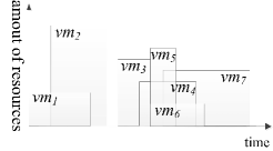
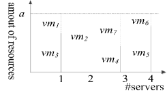
(a) VM requests

(b) Solution under the classic model

6cm][b].5

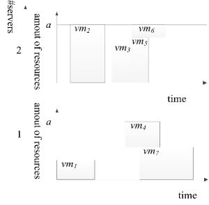
(c) Solution under the CDBP model

Figure 1: Schematic illustrations of the classic and CDBP models

To provide an intuitive description of the proposed model, the allocation results obtained in the classic setting and in the CDBP setting are presented in Figure 1(b) and Figure 1(c), respectively, given the VM requests in Figure 1(b). In Figure 1, rectangles are used to represent the VMs, with the height representing the amount of resources, the width representing the duration, and the horizontal position representing the arrival time. To clearly visualize the allocation results, $a$ is used to denote the amount of resources possessed by each server, as shown in Figures 1(b) and 1(c). Note that resources can have multiple dimensions (e.g., CPU, memory, and SSD) and that the servers can be heterogeneous in the present model, although only one dimension is used to represent the resources in Figure 1 to make the figure simpler and more concise. As shown in Figure 1(b), under the classic model, the scheduler must allocate new resources for each VM because of the lack of time information. By contrast, as Figure 1(c) indicates, the CDBP model allows different VMs, for example, $vm_{2}$ and $vm_{3}$, to occupy the same resources in different periods to reduce the required #servers. The resultant #servers required to accept all requests is 4 in the classic setting and 2 in the CDBP setting. Thus, it can be concluded that the CDBP model can decrease the total #servers required to accept all requests by means of time multiplexing.

There are several special forms available for requests in the proposed model, as follows:

1. arrival time $=0$: the request should be executed immediately, without a reservation.

2. execution time $=\infty$: the duration of the request is undetermined, and the demanded resources should be reserved until it terminates.

3. arrival time $=0$ and execution time $=\infty$: the request will be degraded into a classic request since it does not provide any valid time information.

The use of these three special forms in the CDBP model is not recommended because they will reduce the degree of time multiplexing. In addition, from the third form, we find that the request under the CDBP model is more general than the original one, which indicates a wider range of application.

As shown in Equation 1, the aim is to minimize the #servers, thus reducing the upfront cost, while accepting all VMs. However, other objectives (e.g., load balancing and cost minimization) can also be adopted. Section 4 will present the algorithms proposed to address the VMP problem with an additional time dimension derived from the heterogeneous and multidimensional CDBP model introduced in this section.

4 Scheduling Algorithms

To handle the problem derived from the model proposed in Section 3, this section proposes DCBB algorithm and improves the state-of-the-art algorithm OEMACS and the classic algorithm DDFF. First, the motivations for and requirements of the algorithms for use within our proposed heterogeneous and multidimensional CDBP model are introduced. Then, we present the improved versions of DDFF and OEMACS, namely, DDFF⁺ and OEMACS⁺, that have been adapted for use within the proposed model. Finally, the DCBB procedure and its theoretical analysis are shown.

4.1 Motivations and Requirements

Although various algorithms for the classic VMP problem have been proposed, as described in Section 2, there is a need to design novel algorithms or improve existing algorithms to handle the additional time dimension in the CDBP model. Although the time dimension can be addressed in a time-sequential fashion using the classic online algorithms, their accuracies need to be improved, as shown in Section 5. Therefore, the DCBB algorithm is proposed to effectively and efficiently handle the VMP problem with the additional time dimension. In addition, DDFF and OEMACS are modified for use within the proposed model to observe their performance with additional time information and to compare them with the proposed DCBB algorithm.

A practical VMP algorithm under the proposed model should satisfy the following requirements.

1. Multidimensional resources Luo et al (2014): the algorithm should be able to handle resources with multiple dimensions, although some algorithms will become slower as the number of resource dimensions increases.

2. Heterogeneity Luo et al (2014): the algorithm should consider heterogeneous environments, in which servers have different amounts of resources, since such environments are a common feature of cloud datacenters.

3. Time dimension Gu et al (2017): the algorithm should be able to handle the time dimension, which is the key feature of the CDBP model. Time multiplexing should be enabled to increase the resource utilization ratio and thus reduce the #servers required to accommodate VMs.

4. Availability Toosi et al (2015): the algorithm should ensure that resources are reserved in the appointed period for every accepted VM request, which is the basic requirement of the advance reservation mechanism.

The following subsections present the improved algorithms DDFF⁺ and OEMACS⁺ and the proposed algorithm DCBB.

4.2 Duration-Descending First Fit with a Shuffling Process

In the literature, Runtian et al. Ren and Tang (2016) proposed the DDFF and dual-coloring algorithms to minimize the total usage time of servers under the CDBP model, with approximation ratios of 5 and 4, respectively. In this subsection, the aim is to modify the DDFF algorithm to minimize the #servers in a heterogeneous environment with multidimensional resources. Although the dual-coloring algorithm has a lower approximation ratio, the difficulty of enhancing it to consider multidimensional resources impedes its application to our proposed model. DDFF first sorts the VMs in descending order by duration and then allocates the VMs in an FF manner. It can be easily adapted to a scenario with multidimensional resources because of its natural features. However, FF-based algorithms such as DDFF, which were originally designed for scenarios with 1 resource dimension, generally have difficulty sorting servers by their resources in a multidimensional-resource scenario since no inclusion relationship exists in this case. Inspired by Liu et al (2016), DDFF⁺ has been designed as an improved version of DDFF with an additional shuffling process to improve the scheduling performance. In addition, FF⁺ has been designed using a similar improvement technique, although the detailed procedure is not presented here to avoid repetition. The pseudocode for DDFF⁺ with a shuffling process is shown in Algorithm 1.

1

Input: a set of $n$ VMs, $vmSet$; a set of $m$ servers, $serverSet$

Output: an allocation of the VM requests in $vmSet$ to the servers in $serverSet$

2

3$vmSet$ $\leftarrow\textnormal{{descendingSortByDuration}}(\textnormal{{$vmSet$}})$ $O(nlogn)$

4 $serverSet$ $\leftarrow\textnormal{{shuffle}}(\textnormal{{$serverSet$}})$ $O(m)$

5 $allocation\leftarrow\emptyset$ $O(1)$

6 foreach  $vm$ in $vmSet$ do

7      foreach  $server$ in $serverSet$ do

8            if $server.\textnormal{{canAccommodate}}(vm)$ then

9                  $allocation.\textnormal{{add}}(\{server,vm\})$ $O(1)$

10            

11      

12

return $allocation$

Algorithm 1 DDFF⁺

In Line 1 of Algorithm 1, the VMs are sorted in descending order by duration, with the aim of improving the accuracy of the algorithm. In Line 2, the servers are shuffled to improve the scheduling performance in multidimensional-resource scenarios (R1) and heterogeneous environments (R2). The effectiveness of the sorting and shuffling processes has been demonstrated through experiments (Section 5). When the algorithm judges whether a server can accommodate a VM, as shown in Line 6, every resource dimension (R1) and the time dimension (R3) are simultaneously considered. Once a server that can accommodate the VM is found, the corresponding demanded resources will be reserved for the VM (R4), as shown in Line 7.

Now that the details of DDFF⁺ have been introduced, it can be proven that it is a polynomial-time algorithm with a time complexity of $O(nlogn)+O(mn)$, where $m$ and $n$ are the #servers and the number of VMs (#VMs), respectively. Although this algorithm has a fast processing speed, its outcome is generally far from the optimum. To compensate for this degradation in accuracy, two more algorithms are presented below that are designed to achieve more accurate scheduling solutions.

4.3 Time-aware and Multidimensional OEMACS

As mentioned in Section 2, the OEMACS algorithm Liu et al (2016) performs better than the conventional heuristics and other evolutionary algorithms when addressing the classic VMP problem in heterogeneous environments (R2). The local search techniques, namely, order exchange and migration, proposed by the authors for the ant colony system contribute to the impressive performance of OEMACS. Inspired by this algorithm, OEMACS⁺ has been designed to consider the additional time dimension (R3) and the possibility of advance reservation (R4), allowing this algorithm to be applied to our proposed heterogeneous and multidimensional CDBP model. Furthermore, OEMACS⁺ is also enhanced in terms of its consideration of multidimensional resources (R1), whereas OEMACS was originally designed for only two resource dimensions. To achieve the above goals, the majority of OEMACS was preserved, with the main modifications being concentrated in only a few formulae. The modified formulae are shown in Equations 6, 7, 8, 9 and 10, and the notations used are explained in Table 3.

Table 3: List of notations used to describe OEMACS⁺

Notation	Definition
$D$	The set of resource dimensions
$M_{t}$	The set of servers utilized at time $t$
$P_{id}$	The total amount of the $d^{th}$ resource possessed by the $i^{th}$ server
$R_{itd}$	The remaining amount of the $d^{th}$ resource of the $i^{th}$ server available at time $t$
$S$	A solution to the VMP problem
$S_{b}$	The best solution in the current iteration
$T(i)$	The execution period of the $i^{th}$ VM
$v_{id}$	The amount of the $d^{th}$ resource demanded by the $i^{th}$ VM
$y_{i}$	A variable indicating whether the $i^{th}$ server is used ($y_{i}=1$) or not ($y_{i}=0$)

1. The expression for identifying feasible servers is modified to ensure that the total amount of resources demanded by all VMs is not larger than the capacity of the target server in every resource dimension at any time, as shown in Equation 6.

   $$I{{{}^{\prime}}_{j}}=\left\{\left.i\left|{{R}_{itd}}\geq{{v}_{jd}},1\leq i\leq{{M}_{t}},\forall t\in T(j),\forall d\in D\right|\right\}\right.$$ (6)

2. The expressions for the heuristic information (Equation 7), overload ratio (Equation 8), heuristic objective (Equation 9) and global pheromone updating operation (Equation 10) are improved by calculating the average remaining resource ratio during a time period considering all resource dimensions, as shown below.

   $$\eta^{\prime}(i,j)=\frac{1-\frac{\sum\limits_{{{d}_{1}}\in D}{\sum\limits_{\begin{smallmatrix}{{d}_{2}}\in D\\ {{d}_{1}}\neq{{d}_{2}}\end{smallmatrix}}{\left|\frac{1}{{{P}_{id{{}_{1}}}}}\left(\frac{\sum\limits_{t\in T(j)}{{{R}_{i}}_{t{{d}_{1}}}}}{|T(j)|}-{{v}_{j{{d}_{1}}}}\right)-\frac{1}{{{P}_{id{{}_{2}}}}}\left(\frac{\sum\limits_{t\in T(j)}{{{R}_{i}}_{t{{d}_{2}}}}}{|T(j)|}-{{v}_{j{{d}_{2}}}}\right)\right|}}}{\text{C}_{\left|D\right|}^{2}}}{\frac{\sum\limits_{d\in D}{\left|\frac{1}{{{P}_{id}}}\left(\frac{\sum\limits_{t\in T(j)}{{{R}_{i}}_{td}}}{|T(j)|}-{{v}_{jd}}\right)\right|}}{\left|D\right|}\text{+}1.0}$$ (7)

   
   

   $$over^{\prime}(i)=\sum\limits_{d\in D}{\left|\frac{1}{{{P}_{id}}}\left(\frac{\sum\limits_{t\in T(j)}{{{R}_{i}}_{td}}}{|T(j)|}-v_{jd}\right)\right|}$$ (8)

   
   

   $$f{{{}^{\prime}}_{2}}(S)=\sum\limits_{i\in{{M}_{t}}}{\left(\sum\limits_{d\in D}{\left(\left|\frac{1}{{{P}_{id}}}\left(\frac{\sum\limits_{t\in T(j)}{{{R}_{i}}_{td}}}{|T(j)|}\right)\right|\right)}\cdot{{y}_{i}}\right)}$$ (9)

   
   

   $$\Delta\tau{{{}^{\prime}}_{i}}=\frac{1}{{{f}_{1}}({{S}^{b}})}+\frac{1}{\sum\limits_{d\in D}{\frac{1}{{{P}_{id}}}\left(\frac{\sum\limits_{t\in T(j)}{{{R}_{i}}_{td}}}{|T(j)|}\right)}+1}$$ (10)

Through the modifications shown in Equations 6, 7, 8, 9 and 10, OEMACS⁺ can be applied in our proposed heterogeneous and multidimensional CDBP model for enhancing the classic ant colony system with order exchange and migration as local search techniques. A brief explanation of the modified formulae is presented here, and the reader can refer to Liu et al (2016) for more details. First, Equation 6 is used to select the feasible servers that have sufficient resources for the VM. Then, the heuristic information that is used to guide the greedy search is calculated using Equation 7. The overload ratio calculated in Equation 8 represents the difference between the required and total resources after a VM has been accommodated. Then, the heuristic objective expressed in Equation 9 is used to evaluate the solution. Finally, Equation 10 is used to calculate the global pheromone, which guides the construction of better solutions.

4.4 Branch-and-Bound Algorithm with a Divide-and-Conquer Strategy

Although the classic BB algorithm can yield the optimal solution when applied to the linear programming model introduced in Section 3, its execution time is beyond tolerance, especially in large-scale cases. In this subsection, we propose the DCBB algorithm, which is based on the BB algorithm and includes an additional divide-and-conquer process to improve the scheduling efficiency with little to no degradation in accuracy. To achieve this goal, DCBB first clusters the VMs into several VM sets, then works out the scheduling solutions for each set, and finally merges these subsolutions into the final one.

The main DCBB procedure is as follows.

1. Cluster the VMs into a set of clustered sets (SCS) that satisfy the following conditions:

   1. The execution times of every two VMs in the same clustered set (CS) overlap with each other.

   2. The execution times of any two VMs in different CSs do not overlap.

   Then, place the VMs that cannot be clustered into any CS into the left set (LS).

2. Schedule the VMs in different CSs separately with BB.

3. Schedule the VMs in LS with DDFF⁺.

4. Combine the solutions obtained in Steps 2 and 3.

As shown above, rather than scheduling the VMs as a unit, the DCBB algorithm employs a divide-and-conquer strategy to handle the problem more efficiently. Step 1 enables time multiplexing (R3) by clustering the VMs into several VM sets based on time information. Then, these sets of VMs are scheduled separately in Steps 2 and 3, and finally, the subsolutions are merged without resource contention (R4) in Step 4. Although the original BB algorithm can be used to solve the VMP problem with multidimensional resources (R1) in heterogeneous environments (R2), it is computationally prohibitive. Through the divide-and-conquer process, DCBB achieves significantly improved efficiency at the cost of a minor degradation in precision, as demonstrated in Section 5.

Input: a set of VM requests, $vmSet$; a set of servers, $serverSet$

Output: an allocation of the VM requests in $vmSet$ to the servers in $serverSet$

// Cluster the VMs into the SCS and LS. A typical clustering algorithm is presented in Algorithm 3

1 ($scs$, $ls$) $\leftarrow\textnormal{{cluster}}(\textnormal{{$vmSet$}})$

2foreach  $cs$ in $scs$ do

3      $allocation\leftarrow allocation\cup\textnormal{{BB}}(\textnormal{{$cs$}},\textnormal{{$serverSet$}})$

4

5$allocation\leftarrow allocation\cup\textnormal{{DDFF}}^{+}(\textnormal{{$ls$}},\textnormal{{$serverSet$}})$

return $allocation$

Algorithm 2 DCBB

1

2

Input: a set of VM requests, $vmSet$

Output: SCS $scs$; LS $ls$

3

4$scs$ $\leftarrow\emptyset$, $ls$ $\textnormal{{$\leftarrow$}}\emptyset$

5while $|\textnormal{{$vmSet$}}|\neq 0$ do

       // determine the time $t$ when the most VMs will be running

6       $t\textnormal{{$\leftarrow$}}\textnormal{{findTimeMostVmsContaining}}(\textnormal{{$vmSet$}})$

       // put all remaining VMs whose execution times contain $t$ into $cs$

7       $\textnormal{{$cs$}}\textnormal{{$\leftarrow$}}\textnormal{{getVMSetContainingTime}}(t,\textnormal{{$vmSet$}})$

8       $scs$ $\leftarrow$ $scs$ $\cup$ $cs$

9      $vmSet$ $\leftarrow$ $vmSet$ \$cs$

10      

11      foreach  $vm_{1}$ in $vmSet$ do

12            foreach  $vm_{2}$ in $cs$ do

                  // $\textnormal{{p}}(v)$ represents the execution time of VM $v$

13                   if $\textnormal{{p}}(vm_{1})\cap\textnormal{{p}}(vm_{2})\neq\emptyset$  then

14                        $ls$ $\leftarrow$ $\textnormal{{$ls$}}\cup\{vm_{1}\}$

15                         $vmSet$ $\leftarrow$ $vmSet$ \{$vm_{1}$}

16                  

17            

18      

return $scs$, $ls$

Algorithm 3 Most-Greedy Clustering Algorithm

The pseudocode for DCBB is shown in Algorithm 2. In this algorithm, Line 1 corresponds to the clustering process, while Lines 2 to 5 represent the processes of solving and merging. Various clustering algorithms have been designed such that the CSs will satisfy the two conditions described in the DCBB procedure. However, in the current work, the different clustering algorithms perform similarly in both the theoretical analysis presented later in this subsection and the experiments we conducted. Thus, only one clustering algorithm, namely, most-greedy clustering (MGC), is presented here to demonstrate the process. The main strategy of MGC is to iteratively find the CS of the maximum size. The pseudocode presented in Algorithm 3 shows that MGC mainly involves the following steps:

1. Build a CS with the largest VM set in which the execution times of every two VMs overlap with each other. (Lines 3-5)

2. Place all remaining VMs whose execution times overlap with that of any VM in a CS into the LS. (Lines 7-11)

3. Repeat Steps 1 and 2 until all VM have been clustered into a set. (Lines 2-11)

Steps 1 and 2 guarantee that the execution times of any two VMs in a CS will overlap with each other and that no two VMs in different CSs will overlap, while Step 3 ensures that all VMs will be clustered into VM sets, based on which they will be scheduled later.

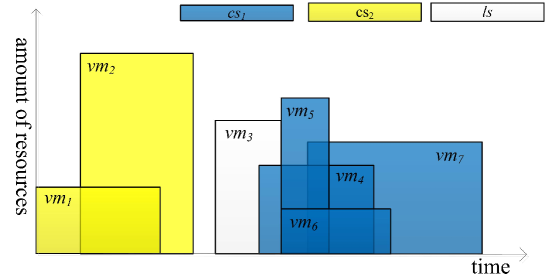
Figure 2: Schematic illustration of MGC

Figure 2 illustrates the clustering results obtained by MGC for 7 VMs. It shows that $vm_{4}–vm_{7}$ constitute the maximal set of overlapping VMs, the size of which is 4. Thus, MGC first puts $vm_{4}–vm_{7}$ into $\textnormal{{$cs$}}_{1}$. Then, $vm_{3}$ is clustered into the $ls$ since its execution time overlaps with that of $vm_{4}$. Finally, MGC clusters $vm_{1}$ and $vm_{2}$ into $\textnormal{{$cs$}}_{2}$ since their execution times overlap.

Although much more theoretical research on DCBB and suitable clustering algorithms needs to be conducted, some of the features of the clustering algorithm and its influence on DCBB have already been discovered, as described by the following lemmas and theorems, in which the abbreviations listed in Table 4 are used.

Table 4: List of abbreviations used to describe DCBB

Abbreviation	Definition
A$(V)$	#servers required by algorithm A for VM set $V$
$ls$	The LS generated by a clustering algorithm
OPT	The optimal algorithm
p$(v)$	The run time of VM $v$
$scs$	The SCS generated by a clustering algorithm

Lemma 1

If one clustering algorithm yields $|\textnormal{{$ls$}}|$ = 0, then all clustering algorithms will yield $|\textnormal{{$ls$}}|$ = 0.

Proof

Assume that the lemma is invalid. Suppose that clustering algorithm $a_{1}$ yields SCS $\textnormal{{$scs$}}_{1}=\{\textnormal{{$cs$}}_{11},\textnormal{{$cs$}}_{12},...,\textnormal{{$cs$}}_{1n}\}$ and that clustering algorithm $a_{2}$ yields SCS $\textnormal{{$scs$}}_{2}=\{\textnormal{{$cs$}}_{21},\textnormal{{$cs$}}_{22},...,\textnormal{{$cs$}}_{2n}\}$ and LS $ls^{\prime}$. Then, for any $v_{i}\in ls^{\prime}$, there must exist two VMs $v_{k_{1}}$ and $v_{k_{2}}$ belonging to the same CS $\textnormal{{$cs$}}_{2j}$ in $\textnormal{{$scs$}}_{2}$ that satisfy Equations 11 to 13:

$$\textnormal{{p}}(v_{i})\cap\textnormal{{p}}(v_{k_{1}})=\emptyset,$$ (11)

$$\textnormal{{p}}(v_{i})\cap\textnormal{{p}}(v_{k_{2}})\neq\emptyset,\\$$ (12)

$$\textnormal{{p}}(v_{k_{1}})\cap\textnormal{{p}}(v_{k_{2}})\neq\emptyset.\\$$ (13)

From Equations 12 and 13, it can be inferred that $v_{i}$ and $v_{k_{1}}$ belong to the same $\textnormal{{$cs$}}_{1k}$ since both $v_{i}$ and $v_{k_{1}}$ should belong to the same CS as $v_{k_{2}}$ does in $\textnormal{{$scs$}}_{1}$. However, according to Equation 11, $v_{i}$ and $v_{k_{1}}$ cannot be clustered into the same CS. Thus, the lemma is validated because the assumption fails.

Lemma 2

If the clustering algorithm used in DCBB yields $|ls|$ = 0, then DCBB will produce the optimal solution.

Proof

According to the independence of the execution times of the VMs in different CSs and given $|\textnormal{{$ls$}}|=0$,

$$\text{DCBB}(vmSet)=\text{DCBB}(\underset{\textnormal{{$cs$}}_{i}\in\textnormal{{$scs$}}}{\bigcup}\textnormal{{$cs$}}_{i})=\underset{\textnormal{{$cs$}}_{i}\in\textnormal{{$scs$}}}{max}\text{BB}(\textnormal{{$cs$}}_{i}).$$ (14)

Since

$$\text{BB}(\textnormal{{$cs$}}_{i})\leq\text{BB}(vmSet)\ \text{for}\ \forall\textnormal{{$cs$}}_{i}\in\textnormal{{$scs$}},$$ (15)

the following holds:

$$\text{DCBB}(vmSet)\leq\text{BB}(vmSet).$$ (16)

Since the BB algorithm is ideally accurate, it can be inferred that DCBB yields the optimal solution.

Theorem 4.1

If one clustering algorithm yields $|\textnormal{{$ls$}}|=0$, then $DCBB$ integrated with any clustering algorithm will yield the optimal solution.

Proof

Theorem 4.1 can be deduced based on Lemma 1 and Lemma 2.

Lemma 3

If clustering algorithm $a$ yields $|\textnormal{{$ls$}}|$ = 0 and the VMs $v_{a}$ and $v_{b}$ are clustered into the same CS $\textnormal{{$cs$}}_{i}$ by algorithm $a$, then $v_{a}$ and $v_{b}$ will be clustered into the same CS by all clustering algorithms.

Proof

Assume that $v_{a}$ and $v_{b}$ are clustered into different CSs produced by a certain clustering algorithm. Then, $\textnormal{{p}}(v_{a})\cap\textnormal{{p}}(v_{b})=\emptyset$. However, it can be inferred that $\textnormal{{p}}(v_{a})\cap\textnormal{{p}}(v_{b})\neq\emptyset$ since $v_{a}$ and $v_{b}$ are both clustered into $\textnormal{{$cs$}}_{i}$ by algorithm $a$, which leads to a contradiction.

Lemma 4

If one clustering algorithm results in $|\textnormal{{$ls$}}|$ = 0, then all clustering algorithms will yield the same results.

Proof

For any two clustering algorithms $a_{1}$ and $a_{2}$, if $a_{1}$ yields $\textnormal{{$scs$}}_{1}=\{\textnormal{{$cs$}}_{11},$ $\textnormal{{$cs$}}_{12},…,\textnormal{{$cs$}}_{1m}\}$, then $a_{2}$ yields $\textnormal{{$scs$}}_{2}=\{\textnormal{{$cs$}}_{21},\textnormal{{$cs$}}_{22},…,\textnormal{{$cs$}}_{2n}\}$ without the LS because of Lemma 1. Assume that $v_{x}$ belongs to $\textnormal{{$cs$}}_{1i}$ and $\textnormal{{$cs$}}_{2j}$. If $\textnormal{{$cs$}}_{1i}$ is different from $\textnormal{{$cs$}}_{2j}$, then a VM $v_{y}$ must exist such that either $v_{y}\in\textnormal{{$cs$}}_{1i}$ and $v_{y}\notin\textnormal{{$cs$}}_{2j}$ or $v_{y}\notin\textnormal{{$cs$}}_{1i}$ and $v_{y}\in\textnormal{{$cs$}}_{2j}$. Thus, $v_{x}$ and $v_{y}$ are clustered into the same CS only in $\textnormal{{$scs$}}_{1}$ or $\textnormal{{$scs$}}_{2}$, which contradicts Lemma 3.

Theorem 4.2

$\text{DCBB}(vmSet)\leq\text{OPT}(vmSet)+|\textnormal{{$ls$}}|$.

Proof

The proof can be divided into two separate cases:

1. When $|\textnormal{{$ls$}}|=0$, $\text{DCBB}(vmSet)=\text{OPT}(vmSet)$ according to Lemma 1.

2. When $|\textnormal{{$ls$}}|>0$, let $vmSet^{\prime}=vmSet-|\textnormal{{$ls$}}|$. Since $vmSet^{\prime}$ can be clustered into CSs, the following equation is satisfied according to Lemma 1:

   $$\begin{split}\text{DCBB}(vmSet^{\prime})&=\text{OPT}(vmSet^{\prime})\\ &\leq\text{OPT}(vmSet)\end{split}$$ (17)

   The worst case for DDFF($vmSet$) is $|\textnormal{{$ls$}}|$ when each VM in $ls$ needs to be scheduled to a different server. Thus, it can be inferred that

   $$\begin{split}\text{DCBB}(vmSet)&=\text{DCBB}(vmSet^{\prime}\cup\textnormal{{$ls$}})\\ &\leq\text{DCBB}(vmSet^{\prime})+\text{DDFF}(\textnormal{{$ls$}})\\ &\leq\text{OPT}(vmSet)+|\textnormal{{$ls$}}|\end{split}$$ (18)

Consequently, Theorem 4.2 is satisfied for any $|\textnormal{{$ls$}}|$.

As shown above, no resource-related features are involved in the deductions of Lemmas 1, 2, 3 and 4 and Theorem 4.1, which indicates that the conclusions satisfy requirements R1 and R2 well. Furthermore, Theorem 4.1, Lemma 1, and Lemma 2 represent the typical conditions under which R3 can be best fulfilled. Since all VMs can be clustered into several independent VM sets that do not overlap with each other, DCBB can achieve the optimal solution by merging the subsolutions for each subset under these conditions. Moreover, because all the VMs can be clustered into either a certain CS or the LS, based on which they will later be scheduled to a certain server, R4 is not violated during the clustering process. In addition, Theorem 4.2 presents the upper bound of our proposed DCBB algorithm.

5 Implementation and Experiments

In this section, experimental results are presented to evaluate and compare various algorithms, including BB, DCBB, OEMACS⁺, DDFF⁺, and FF⁺, in our proposed heterogeneous and multidimensional CDBP model. The main metrics used for evaluation are the accuracy and execution time of each algorithm. As mentioned in Section 2, the scheduling problem in the proposed model is NP-hard; thus, obtaining an optimal solution (the least #servers required) in a reasonable time is computationally infeasible. Therefore, as widely adopted in the literature Xiao et al (2015); Gupta and Amgoth (2018); Luo et al (2014); Liu et al (2016); Quang-Hung et al (2013), we assess the accuracy on the basis of the #servers, where a smaller #servers indicates a higher accuracy. In the following, Section 5.1 first introduces the workloads. Then, Sections 5.2, 5.3, 5.4, 5.5 and 5.6 describe experiments conducted to answer the following questions:

1. How do the algorithms perform on a real-world workload? (Section 5.2)

2. What are the convergence rates of search-based algorithms, such as DCBB, BB, and OEMACS⁺, under the proposed model? (Section 5.3)

3. How does the shuffling process affect the performance of FF-based algorithms in a multidimensional environment? (Section 5.4)

4. How do the performances of the algorithms change with increasing problem scale? (Section 5.5)

5. How do time factors (i.e., the arrival times and durations of VMs) affect the performances of the algorithms? (Section 5.6)

Finally, Section 5.7 summarizes the experimental results.

5.1 Workloads

A real-world workload is considered to observe the practical performances of the algorithms. In addition, synthetic workloads are generated to observe the influence of the #VMs and time distribution on the algorithms. Furthermore, as shown in Table 5, 8 types of VMs were selected from the Amazon Elastic Compute Cloud (EC2) to serve as workloads, and 3 types of servers were selected on the basis of the products available from Inspur Technologies Co., Ltd. , to make the experimental environment more similar to a real-world scenario. The selected types of both VMs and servers include CPU-intensive, memory-intensive and SSD-intensive representatives to cover a general set of cases.

Table 5: Types of servers and VMs

	#(V)CPUs	Memory (GB)	SSD (GB)
servers	16	32	160
	8	32	160
	8	64	320
VMs	1	3.75	4
	2	7.5	32
	4	15	80
	2	3.75	32
	4	7.5	80
	8	15	160
	2	15.25	32
	4	30.5	80

In addition, a uniform distribution $U(a,b)$ and a Gaussian distribution $N(\mu,\sigma^{2})$ are used to simulate the arrival times and durations, respectively of the VMs.

The details of the workloads are as follows.

• Workload I: real-world workload
  Considering the completeness and quality of the workloads, we selected two real-world datasets, namely, “RICC” and “UniLuGaia”, from the “Logs of Real Parallel Workloads from Production Systems” Feitelson (2017) to evaluate and compare the accuracy and efficiency of the algorithms. In contrast to synthetic data, these real-world datasets have long time spans, sparse VM distributions, and occasionally incomplete records. Thus, data cleaning was first performed on the two datasets to improve the significance of the experiments. Considering the computational capacity of the experimental environment, 500 qualified records extracted from each dataset were used to conduct the experiments.

• Workload II: varying #VMs and fixed time distributions
  Workload II, in which the total #VMs varies from 24 to 336 while the distributions of the VM arrival times and durations are fixed, as shown in Table 6, was generated to illustrate the influence of the #VMs.

  Table 6: Distributions of the arrival times and durations of the VMs and their default parameters

  Type	Distribution	Parameter $1$	Parameter $2$
  Arrival time	Uniform	$0$ $(a)$	$240$ $(b)$
  Duration	Gaussian	$360$ $(\mu)$	$60$ $(\sigma)$

• Workload III: fixed #VMs and varying time distributions
  Workload III was designed to study the influence of time distributions on the algorithms. The total #VMs of this workload is fixed at 160. For the time distributions, both the upper bound $b$ on the arrival times and the mean duration $\mu$ vary between 60 s and 420 s, while the lower bound $a$ on the arrival times and the variance $\sigma$ of the durations remain unchanged, as shown in Table 6.

The scheduling algorithms were evaluated and compared using the above workloads in a KVM-based VM with 8 VCPUs and 16 GB of memory. A private cloud platform was built using OpenStack to observe the performances of the proposed model and algorithms. A simulated environment was also established in which to conduct large-scale experiments. In the following sections, we do not differentiate the real and simulated experimental environments since they do not affect the scheduling results.

5.2 Experiment on the Real-World Workload

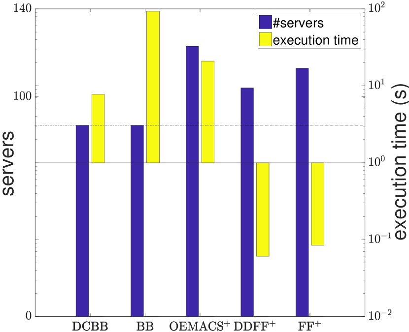
(a) RICC dataset

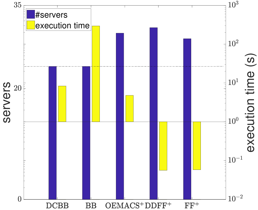
(b) UniLuGaia dataset

Figure 3: Comparisons of the algorithms using real-world datasets. The fewest #servers achieved by the algorithms are marked with dotted lines.

In this subsection, Workload I is employed to check the performances of the algorithms on real-world datasets, which is a key component of the evaluation and comparison. The results are shown in Figure 3, with dotted lines indicating the fewest #servers required by the algorithms.

First, the execution times are compared. As shown, DDFF⁺ and FF⁺ require less than 0.1 s to yield the solutions, which is much less than the times required by the other algorithms. The execution times of DCBB and OEMACS⁺ are approximately dozens of seconds, whereas BB requires the most time – several hundreds of seconds.

In terms of the #servers required by each algorithm, DCBB and BB achieve the optimal results, requiring 19.46% and 20.13% fewer servers on average than the DDFF⁺ and FF⁺ algorithms do, respectively. DDFF⁺ requires the third fewest servers on the RICC dataset; however, it has the worst accuracy on the UniLuGaia dataset. OEMACS⁺ and FF⁺ have accuracies similar to that of DDFF⁺.

To summarize, DCBB achieves the same optimal solution as BB does with an execution time that is an order of magnitude shorter. Moreover, OEMACS⁺ requires nearly the largest #servers with a relatively long execution time, which may be caused by the additional problem complexity introduced by the additional time and resource dimensions. Furthermore, the FF-based algorithms can produce a scheduling solution within a trivial execution time, indicating that they are suitable for real-time scheduling. In the following subsections, more comprehensive analyses of the algorithms will be presented based on synthetic data.

5.3 Convergence Rate Comparison

As search-based algorithms, DCBB, BB, and OEMACS⁺ can deliver better solutions given longer execution times, up to the time when the optimal solution is found. In particular, BB can theoretically always produce an optimal scheduling solution given enough time. However, the execution time cannot be arbitrarily long. Thus, the convergence rates of these algorithms should be studied to evaluate their performance and achieve a suitable compromise between accuracy and efficiency. In this subsection, DCBB, BB, and OEMACS⁺ are applied to Workload II to compare the convergence rates of these algorithms.

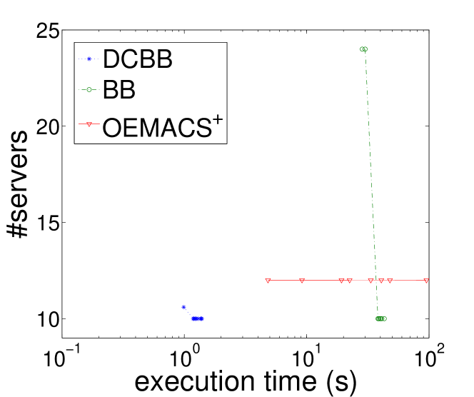
(a) #VMs = 24

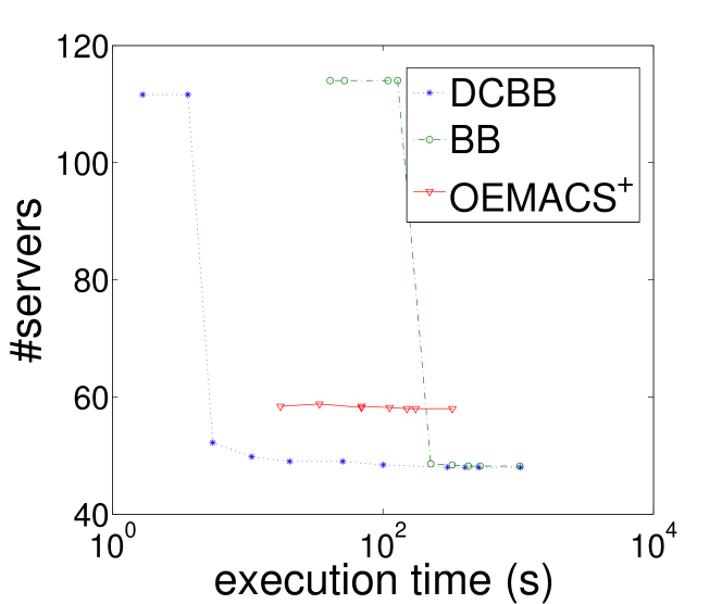
(b) #VMs = 120

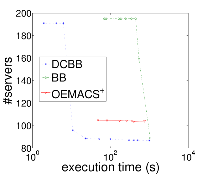
(c) #VMs = 216

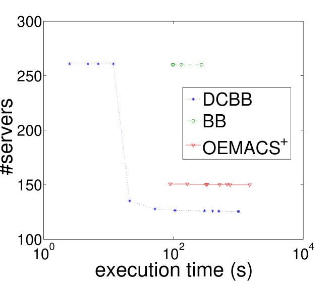
(d) #VMs = 312

Figure 4: Comparison of the convergence rates

Figure 4 shows that the total #servers required by DCBB decays exponentially with an increasing execution time, and thus, the convergence rate of this algorithm becomes the fastest. Furthermore, DCBB converges before 50 s in most cases. In contrast, the convergence rate of BB is much slower, with a nearly linear decay after a period of unchanging results. The missing data of BB after 50 s in Figure 4(d), where the #VMs is 312, is caused by the excessive computational resource requirements of this algorithm. In the other cases shown in Figures 4(a), 4(b) and 4(c), BB obtains nearly convergent results after 1000 s. For OEMACS⁺, the #servers required remains almost unimproved as the execution time increases.

It can be concluded that DCBB achieves the fastest convergence rate, OEMACS⁺ yields nearly unchanging results over time, and BB has the slowest convergence rate. In the following subsections, time limits of 50 s and 1000 s are set for DCBB and BB, respectively, and an iteration limit of 5 is set for OEMACS⁺ to balance the accuracy and efficiency of these algorithms according to the results shown in Figure 4.

5.4 Effectiveness of Shuffling

In this subsection, the improved algorithms FF⁺ and DDFF⁺ are compared with the original algorithms FF and DDFF using Workload II to observe the effectiveness of the shuffling process.

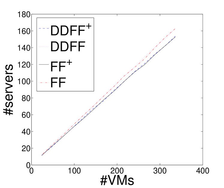
(a) Effect of shuffling on #servers

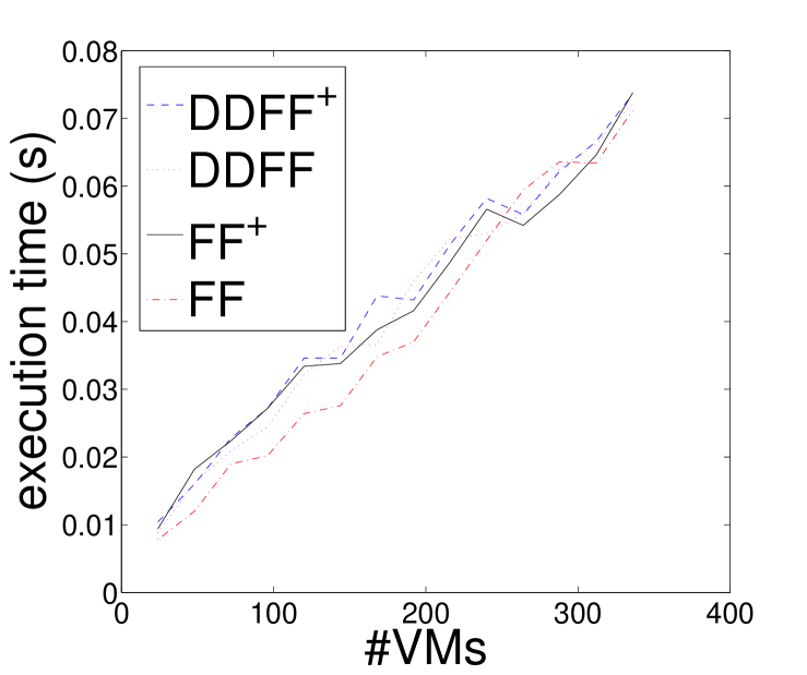
(b) Effect of shuffling on execution time

Figure 5: Effects of the shuffling process

In Figure 5(a), the lines representing the #servers required by FF⁺ and DDFF⁺ lie below those for FF and DDFF, indicating that the shuffling process reduces the total #servers required. Moreover, the effectiveness of the shuffling process becomes more evident as the #VMs increases. Furthermore, the two nearly overlapping lines in Figure 5(a) indicate that the duration-descending process does not have much impact on the #servers under our proposed heterogeneous and multidimensional CDBP model.

Regarding the execution time, Figure 5(b) implies that the shuffling process does not incur much extra time. Although FF and DDFF require shorter execution times when the #VMs is small, the difference disappears as the #VMs increases. The extra execution time incurred by the shuffling process is thus regarded as trivial compared to the time required for the total scheduling process and the perturbations caused by different server orders.

From the experimental results in this subsection, it can be concluded that the shuffling process can slightly reduce the #servers required by FF and DDFF. Moreover, the additional time incurred by the shuffling process is trivial, particularly when the #VMs is large.

5.5 Influence of the Number of Virtual Machines

In this subsection, the algorithms are evaluated and compared on workload II, in which the #VMs varies. Table 7 lists the average #servers and execution time of each algorithm for each #VMs. Data for BB are not available when the #VMs exceeds 240 because the computational resources of the experimental environment are no longer sufficient to support BB in these cases.

Table 7: Evaluations and comparisons of the algorithms with various #VMs. #S and T denote the #servers and the execution time, respectively. The fewest #servers and the shortest execution time achieved among all algorithms are marked with underscores and bold text, respectively.

#VMs	DCBB		BB		OEMACS+		DDFF+		FF+
	#S	T (s)	#S	T (s)	#S	T (s)	#S	T (s)	#S	T (s)
24	10.0	1.2	10.0	39.0	12.0	4.8	11.6	0.010	11.4	0.009
48	20.0	45.8	19.8	831.0	23.6	8.3	22.0	0.016	22.6	0.018
72	29.2	33.2	29.0	479.1	34.8	9.7	33.2	0.023	33.2	0.022
96	39.0	50.4	39.0	1049.5	46.4	15.5	44.4	0.027	44.4	0.027
120	49.0	50.5	48.2	1027.6	58.4	17.5	55.8	0.035	54.8	0.033
144	59.0	50.6	58.0	1034.4	69.2	22.9	67.2	0.035	65.8	0.034
168	68.0	51.3	67.8	1037.2	81.2	28.1	76.4	0.044	77.6	0.039
192	78.4	52.7	78.4	1044.6	92.6	37.6	88.8	0.043	87.8	0.042
216	88.0	51.9	89.0	1053.8	104.8	48.4	99.4	0.051	99.6	0.049
240	97.8	50.9	98.0	1051.8	115.6	51.5	111.0	0.058	110.6	0.057
264	110.0	52.3	NaN	NaN	126.6	68.4	121.0	0.056	119.6	0.054
288	118.8	52.4	NaN	NaN	138.8	76.2	132.2	0.062	131.6	0.059
312	127.6	51.9	NaN	NaN	150.6	89.4	142.0	0.067	142.2	0.065
336	139.8	56.4	NaN	NaN	162.4	88.8	153.8	0.074	152.8	0.074

Table 7 shows that DCBB yields better results than DDFF⁺, FF⁺, and OEMACS⁺ do in much less time than that required by BB. Although BB generally yields a slightly smaller #servers than DCBB does when the #VMs is less than 192, it requires a longer execution time and an enormous amount of computational resources. Furthermore, DCBB yields the smallest #servers when the #VMs exceeds 192. The performance of OEMACS⁺ is not desirable, as it often requires both the largest #servers and a relatively long execution time. In addition, DDFF⁺ and FF⁺ always output similar results for the #VMs in less than 0.1 s, which is a trivial execution time compared to those of the other algorithms.

The results in this subsection show that a larger #VMs can cause an increase in the resulting #servers. Moreover, BB yields the smallest #VMs, though with a long execution time, when the problem scale is small. However, ideally accurate algorithms (e.g., BB) cannot handle large-scale problems because of their prohibitive computational complexity. In addition, this experiment demonstrates that DCBB can achieve a suitable tradeoff between accuracy and efficiency, as it can output near-optimal results within 60 s. Although DDFF⁺ and FF⁺ do not yield better results than that of DCBB, they can produce a scheduling solution within less than 0.08 s, which is suitable for real-time scheduling.

5.6 Influence of Time Factors

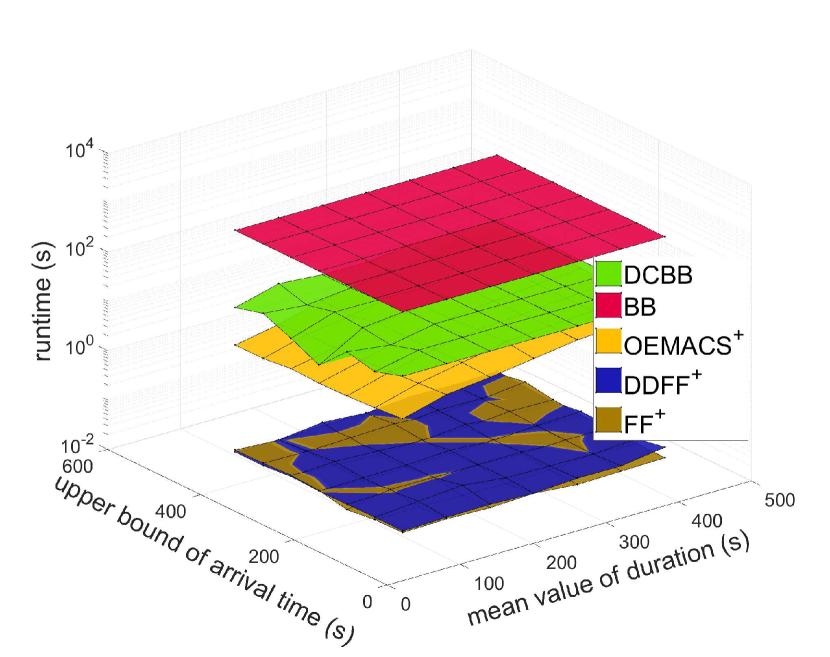
(a) Execution times required by the algorithms under different VM time configurations

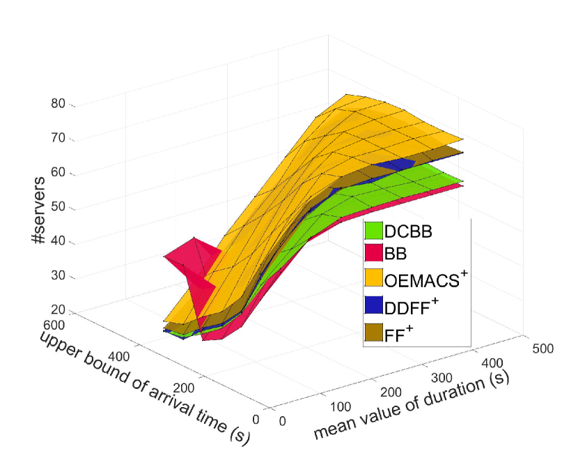
(b) #servers required by the algorithms under different VM time configurations

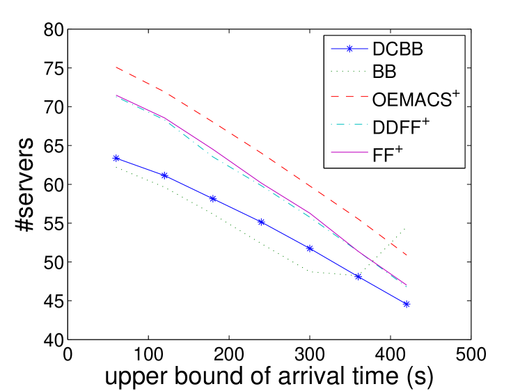
(c) #servers required versus the arrival time range

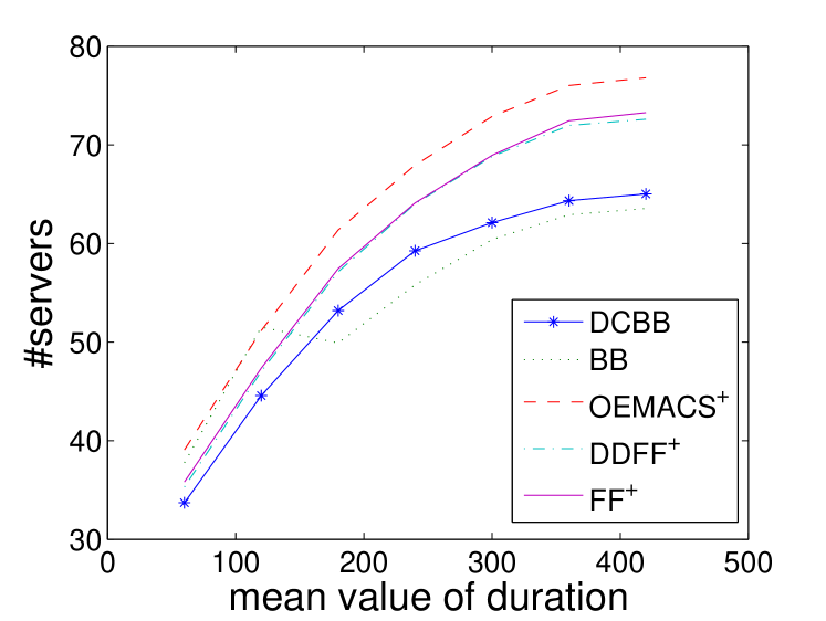
(d) #servers required versus the mean duration

Figure 6: Evaluations and comparisons of the algorithms with various VM time distributions

To investigate the influence of the VM arrival times and durations, the results obtained by the algorithms on Workload III, with varying distributions of the arrival times and durations of the VMs, are presented to show the resulting changes in the accuracy and efficiency of the different algorithms. Figure 6 compares the results obtained with various upper bounds on the arrival time and various mean durations.

As shown in Figure 6(a), the execution times of the algorithms do not change much with the variation of the time factors. Consistent with the previous results, BB takes the most time (approximately 1020 s), while DDFF⁺ and FF⁺ require only a trivial execution time (less than 0.1 s). Because BB does not terminate before the time limit (1000 s) is reached, it does not guarantee an optimal result.

From a comprehensive analysis of Figures 6(b), 6(c) and 6(d), it can be concluded that a shorter duration and a wider arrival time range both result in a lower #servers required by algorithms. These results are logical, as a sparser distribution of VMs can lead to a higher degree of time multiplexing, thus contributing to a smaller #servers. Although BB generally requires the fewest #servers, its execution time is long. Moreover, several outliers are produced by BB, as seen in Figure 6(b), reflecting its instability under a time limit. Similar to the previous results, OEMACS⁺ generally performs the worst in this experiment. Furthermore, DCBB yields the second smallest #servers, as shown in Figures 6(b), 6(c) and 6(d).

To summarize, a shorter duration and a wider arrival time range cause the algorithms to require a lower #servers, possibly because of a higher degree of time multiplexing. The execution time does not vary much with different time parameter settings. Consistent with the previous results, DCBB yields a near-optimal solution within a relatively short execution time, BB achieves the lowest #servers with the longest execution time, OEMACS⁺ typically delivers unsatisfactory performance, and the FF-based algorithms have the fastest processing speed.

5.7 Summary

The experiments presented in Sections 5.2, 5.3, 5.4, 5.5 and 5.6 have answered questions Q1-Q5 posed at the beginning of Section 5:

1. BB and DCBB can both yield the optimal solutions on the real-world datasets considered here; however, DCBB requires an order of magnitude less time than BB does. Meanwhile, FF⁺ and DDFF⁺ can produce a scheduling solution within an insignificant execution time (less than 0.1 s), indicating that they are suitable for real-time scheduling. However, the performance of OEMACS⁺ is not satisfactory in terms of either accuracy or efficiency.

2. DCBB has a much faster convergence rate than that of BB. As for OEMACS⁺, its scheduling solutions show almost no improvement with increasing execution time.

3. The shuffling process improves the accuracy of DDFF and FF with a trivial increase in the execution time.

4. A larger #VMs results in an increase in the #servers required. Furthermore, ideally accurate algorithms such as BB have difficulty handling large-scale problems because of their prohibitive computational complexity.

5. A shorter mean duration and a wider arrival time range for the VMs can result in a lower $\#$servers while exerting little influence on the execution time.

In addition, the experiments also demonstrate that the proposed algorithms satisfy requirements R1-4 mentioned in Section 4.1. Since the algorithms can handle Workloads I-III, for which the resources are multidimensional and the servers are heterogeneous, R1 and R2 are satisfied. Furthermore, R3 is met because different VMs without overlapping execution times can share the same resources. R4 is also fulfilled since no VM requests are rejected in the experiments.

Overall, the experimental data confirm that DCBB can yield near-optimal scheduling solutions while having faster convergence rate than the other evaluated search-based algorithms do. The results also demonstrate that the FF-based algorithms have the fastest processing speed and that BB can produce the best solution when the problem scale is small. In addition, the experimental results for OEMACS⁺ are unsatisfactory, possibly because of the extra problem complexity introduced by the additional time and resource dimensions. Furthermore, a wider arrival time range and a shorter mean duration for the VMs both cause a lower #servers to be required since they enable higher degrees of time multiplexing.

6 Conclusions and Future Work

To lower the expensive upfront cost of private clouds, this paper proposes DCBB, an effective and efficient VMP algorithm that is applicable to the heterogeneous and multidimensional CDBP model, to reduce the #servers required to accommodate VMs. The proposed model and algorithm employ time multiplexing to achieve more efficient and flexible scheduling. Theoretical analyses have been conducted to identify the upper bound and other features of DCBB. The experimental data clearly confirm the superiority of DCBB. It has been verified that DCBB can achieve near-optimal solutions while requiring significantly less execution time (by an order of magnitude on a real-world workload) than the BB algorithm does. The experimental results also show that DCBB has a much faster convergence rate than those of the other search-based algorithms evaluated. Although the BB algorithm can yield the optimal solution in theory, it requires a long execution time and a large amount of computational resources and shows unstable performance when given a time limit. Moreover, the accuracies of the DDFF and FF algorithms have been improved by including an additional shuffling process, and the resulting algorithms can be applied for real-time scheduling because of their trivial processing time. In addition, the experimental results demonstrate that OEMACS⁺ does not deliver the expected performance under the proposed model, possibly because of the extra problem complexity introduced by the additional time and resource dimensions. Furthermore, the experiments indicate that, in addition to a lower #VMs, a shorter mean duration and a wider arrival time range for the VMs can also cause a lower #servers to be required due to the higher degree of time multiplexing that can be achieved in this case.

Although extensive experiments have been conducted to evaluate and compare the algorithms considered here, the superiority of DCBB has not been fully theoretically proven. In addition, the influence of the adopted clustering algorithm on DCBB is not clear. Therefore, further theoretical analysis should be conducted to discover more features of DCBB and to enable further improvements.

References

- (1)
- Mell et al (2011) Mell P, Grance T, et al (2011) The NIST definition of cloud computing
- Framingham (2017) Framingham M (2017) Spending on IT infrastructure for public cloud deployments will return to double-digit growth in 2017, according to IDC; 2017. URL https://www.idc.com/getdoc.jsp?containerId=prUS42454117
- Kim (2017) Kim W (2017) Cloud computing trends: 2017 state of the cloud survey. URL https://www.rightscale.com/blog/cloud-industry-insights/cloud-computing-trends-2017-state-cloud-survey, [Online; accessed 23-January-2018]
- Goyal (2014) Goyal S (2014) Public vs private vs hybrid vs community-cloud computing: A critical review. International Journal of Computer Network and Information Security 6(3):20
- Ficco et al (2017) Ficco M, Di Martino B, Pietrantuono R, Russo S (2017) Optimized task allocation on private cloud for hybrid simulation of large-scale critical systems. Future Generation Computer Systems 74:104–118
- Ramanathan and Latha (2018) Ramanathan R, Latha B (2018) Towards optimal resource provisioning for hadoop-mapreduce jobs using scale-out strategy and its performance analysis in private cloud environment. Cluster Computing pp 1–11
- Ye et al (2017) Ye X, Li J, Liu S, Liang J, Jin Y (2017) A hybrid instance-intensive workflow scheduling method in private cloud environment. Natural Computing pp 1–12
- Toosi et al (2015) Toosi AN, Vanmechelen K, Ramamohanarao K, Buyya R (2015) Revenue maximization with optimal capacity control in infrastructure as a service cloud markets. IEEE transactions on Cloud Computing 3(3):261–274
- de Assuncao and Lefèvre (2017) de Assuncao MD, Lefèvre L (2017) Bare-metal reservation for cloud: an analysis of the trade off between reactivity and energy efficiency. Cluster Computing pp 1–12
- Masdari et al (2016) Masdari M, Nabavi SS, Ahmadi V (2016) An overview of virtual machine placement schemes in cloud computing. Journal of Network and Computer Applications 66:106–127
- Feldman et al (2014) Feldman J, Liu N, Topaloglu H, Ziya S (2014) Appointment scheduling under patient preference and no-show behavior. Operations Research 62(4):794–811
- Irwin et al (2006) Irwin DE, Chase JS, Grit LE, Yumerefendi AR, Becker D, Yocum K (2006) Sharing networked resources with brokered leases. In: USENIX Annual Technical Conference, General Track, pp 199–212
- Lawson and Smirni (2002) Lawson BG, Smirni E (2002) Multiple-queue backfilling scheduling with priorities and reservations for parallel systems. In: Workshop on Job Scheduling Strategies for Parallel Processing, Springer, pp 72–87
- Elmroth and Tordsson (2009) Elmroth E, Tordsson J (2009) A standards-based grid resource brokering service supporting advance reservations, coallocation, and cross-grid interoperability. Concurrency and Computation: Practice and Experience 21(18):2298–2335
- Farooq et al (2005) Farooq U, Majumdar S, Parsons EW (2005) Impact of laxity on scheduling with advance reservations in grids. In: Modeling, Analysis, and Simulation of Computer and Telecommunication Systems, 2005. 13th IEEE International Symposium on, IEEE, pp 319–322
- Chase and Niyato (2017) Chase J, Niyato D (2017) Joint optimization of resource provisioning in cloud computing. IEEE Transactions on Services Computing 10(3):396–409
- Coffman et al (1983) Coffman EG Jr, Garey MR, Johnson DS (1983) Dynamic bin packing. SIAM Journal on Computing 12(2):227–258
- Park and Kim (2017) Park JW, Kim E (2017) Runtime prediction of parallel applications with workload-aware clustering. The Journal of Supercomputing 73(11):4635–4651
- Calheiros et al (2015) Calheiros RN, Masoumi E, Ranjan R, Buyya R (2015) Workload prediction using arima model and its impact on cloud applications’ QoS. IEEE Transactions on Cloud Computing 3(4):449–458
- Gandhi et al (2012) Gandhi A, Chen Y, Gmach D, Arlitt M, Marwah M (2012) Hybrid resource provisioning for minimizing data center SLA violations and power consumption. Sustainable Computing: Informatics and Systems 2(2):91–104
- Usmani and Singh (2016) Usmani Z, Singh S (2016) A survey of virtual machine placement techniques in a cloud data center. Procedia Computer Science 78:491–498
- Panigrahy et al (2011) Panigrahy R, Talwar K, Uyeda L, Wieder U (2011) Heuristics for vector bin packing. research microsoft com
- Gao et al (2013) Gao Y, Guan H, Qi Z, Hou Y, Liu L (2013) A multi-objective ant colony system algorithm for virtual machine placement in cloud computing. Journal of Computer and System Sciences 79(8):1230–1242
- Tang and Pan (2015) Tang M, Pan S (2015) A hybrid genetic algorithm for the energy-efficient virtual machine placement problem in data centers. Neural Processing Letters 41(2):211–221
- Fard et al (2017) Fard SYZ, Ahmadi MR, Adabi S (2017) A dynamic VM consolidation technique for QoS and energy consumption in cloud environment. The Journal of Supercomputing 73(10):4347–4368
- Zheng et al (2016) Zheng Q, Li R, Li X, Shah N, Zhang J, Tian F, Chao KM, Li J (2016) Virtual machine consolidated placement based on multi-objective biogeography-based optimization. Future Generation Computer Systems 54:95–122
- Xiao et al (2015) Xiao Z, Jiang J, Zhu Y, Ming Z, Zhong S, Cai S (2015) A solution of dynamic VMs placement problem for energy consumption optimization based on evolutionary game theory. Journal of Systems and Software 101:260–272
- Vu and Hwang (2014) Vu HT, Hwang S (2014) A traffic and power-aware algorithm for virtual machine placement in cloud data center. International Journal of Grid & Distributed Computing 7(1):350–355
- Kanagavelu et al (2014) Kanagavelu R, Lee BS, Mingjie LN, Aung KMM, et al (2014) Virtual machine placement with two-path traffic routing for reduced congestion in data center networks. Computer Communications 53:1–12
- Gupta and Amgoth (2018) Gupta MK, Amgoth T (2018) Resource-aware virtual machine placement algorithm for IaaS cloud. The Journal of Supercomputing 74(1):122–140
- Liang et al (2014) Liang Q, Zhang J, Zhang Yh, Liang Jm (2014) The placement method of resources and applications based on request prediction in cloud data center. Information Sciences 279:735–745
- Sayeedkhan and Balaji (2014) Sayeedkhan PN, Balaji S (2014) Virtual machine placement based on disk I/O load in cloud. vol 5:5477–5479
- Xu et al (2017) Xu M, Tian W, Buyya R (2017) A survey on load balancing algorithms for virtual machines placement in cloud computing. Concurrency and Computation: Practice and Experience 29(12)
- Anand et al (2013) Anand A, Lakshmi J, Nandy S (2013) Virtual machine placement optimization supporting performance SLAs. In: Cloud Computing Technology and Science (CloudCom), 2013 IEEE 5th International Conference on, IEEE, vol 1, pp 298–305
- Chaisiri et al (2009) Chaisiri S, Lee BS, Niyato D (2009) Optimal virtual machine placement across multiple cloud providers. In: Services Computing Conference, 2009. APSCC 2009. IEEE Asia-Pacific, IEEE, pp 103–110
- Ribas et al (2012) Ribas BC, Suguimoto RM, Montano RA, Silva F, de Bona L, Castilho MA (2012) On modelling virtual machine consolidation to pseudo-Boolean constraints. In: Ibero-American Conference on Artificial Intelligence, Springer, pp 361–370
- Fang et al (2013) Fang S, Kanagavelu R, Lee BS, Foh CH, Aung KMM (2013) Power-efficient virtual machine placement and migration in data centers. In: Green Computing and Communications (GreenCom), 2013 IEEE and Internet of Things (iThings/CPSCom), IEEE International Conference on and IEEE Cyber, Physical and Social Computing, IEEE, pp 1408–1413
- Dong et al (2013) Dong J, Wang H, Jin X, Li Y, Zhang P, Cheng S (2013) Virtual machine placement for improving energy efficiency and network performance in IaaS cloud. In: Distributed Computing Systems Workshops (ICDCSW), 2013 IEEE 33rd International Conference on, IEEE, pp 238–243
- Moreno et al (2013) Moreno IS, Yang R, Xu J, Wo T (2013) Improved energy-efficiency in cloud datacenters with interference-aware virtual machine placement. In: Autonomous Decentralized Systems (ISADS), 2013 IEEE Eleventh International Symposium on, IEEE, pp 1–8
- Luo et al (2014) Luo Jp, Li X, Chen Mr (2014) Hybrid shuffled frog leaping algorithm for energy-efficient dynamic consolidation of virtual machines in cloud data centers. Expert Systems with Applications 41(13):5804–5816
- Liu et al (2016) Liu XF, Zhan ZH, Deng JD, Li Y, Gu T, Zhang J (2016) An energy efficient ant colony system for virtual machine placement in cloud computing. IEEE Transactions on Evolutionary Computation
- Quang-Hung et al (2013) Quang-Hung N, Nien PD, Nam NH, Tuong NH, Thoai N (2013) A genetic algorithm for power-aware virtual machine allocation in private cloud. In: Information and Communication Technology-EurAsia Conference, Springer, pp 183–191
- Agrawal and Tripathi (2015) Agrawal K, Tripathi P (2015) Power aware artificial bee colony virtual machine allocation for private cloud systems. In: Computational Intelligence and Communication Networks (CICN), 2015 International Conference on, IEEE, pp 947–950
- Shi et al (2013) Shi L, Butler B, Botvich D, Jennings B (2013) Provisioning of requests for virtual machine sets with placement constraints in IaaS clouds. In: Integrated Network Management (IM 2013), 2013 IFIP/IEEE International Symposium on, IEEE, pp 499–505
- Coffman Jr et al (2013) Coffman Jr EG, Csirik J, Galambos G, Martello S, Vigo D (2013) Bin packing approximation algorithms: survey and classification. In: Handbook of Combinatorial Optimization, Springer, pp 455–531
- De La Vega and Lueker (1981) De La Vega WF, Lueker GS (1981) Bin packing can be solved within 1+ in linear time. Combinatorica 1(4):349–355
- Bansal et al (2006) Bansal N, Correa JR, Kenyon C, Sviridenko M (2006) Bin packing in multiple dimensions: Inapproximability results and approximation schemes. Mathematics of Operations Research 31(1):31–49
- Han et al (1994) Han BT, Diehr G, Cook JS (1994) Multiple-type, two-dimensional bin packing problems: Applications and algorithms. Annals of Operations Research 50(1):239–261
- Li et al (2014) Li Y, Tang X, Cai W (2014) On dynamic bin packing for resource allocation in the cloud. In: Proceedings of the 26th ACM symposium on Parallelism in algorithms and architectures, ACM, pp 2–11
- Kamali and López-Ortiz (2015) Kamali S, López-Ortiz A (2015) Efficient online strategies for renting servers in the cloud. In: International Conference on Current Trends in Theory and Practice of Informatics, Springer, pp 277–288
- Tang et al (2016) Tang X, Li Y, Ren R, Cai W (2016) On first fit bin packing for online cloud server allocation. In: Parallel and Distributed Processing Symposium, 2016 IEEE International, IEEE, pp 323–332
- Ren and Tang (2016) Ren R, Tang X (2016) Clairvoyant dynamic bin packing for job scheduling with minimum server usage time. In: Proceedings of the 28th ACM Symposium on Parallelism in Algorithms and Architectures, ACM, pp 227–237
- Azar and Vainstein (2017) Azar Y, Vainstein D (2017) Tight bounds for clairvoyant dynamic bin packing. In: Proceedings of the 29th ACM Symposium on Parallelism in Algorithms and Architectures, ACM, pp 77–86
- Gu et al (2017) Gu C, Chen S, Zhang J, Huang H, Jia X (2017) Reservation schemes for IaaS cloud broker: a time-multiplexing way for different rental time. Concurrency and Computation: Practice and Experience 29(16)
- Feitelson (2017) Feitelson D (2017) Parallel workloads archive. URL http://www.cs.huji.ac.il/labs/parallel/workload