On the Spectral Efficiency of Noncooperative Uplink Massive MIMO Systems

Abstract

Massive multiple-input multiple-output (MIMO) systems have been drawing considerable interest due to the growing throughput demands on wireless networks. In the uplink, massive MIMO systems are commonly studied assuming that each base station (BS) decodes the signals of its user terminals separately and linearly while treating all interference as noise. Although this approach provides improved spectral efficiency which scales with the number of BS antennas in favorable channel conditions, it is generally sub-optimal from an information-theoretic perspective. In this work we characterize the spectral efficiency of massive MIMO when the BSs are allowed to jointly decode the received signals. In particular, we consider four schemes for treating the interference, and derive the achievable average ergodic rates for both finite and asymptotic number of antennas for each scheme. Simulation tests of the proposed methods illustrate their gains in spectral efficiency compared to the standard approach of separate linear decoding, and show that the standard approach fails to capture the actual achievable rates of massive MIMO systems, particularly when the interference is dominant.

I Introduction

A major challenge of future wireless systems is to meet the growing throughput demand. A promising method for increasing the spectral efficiency (SE) is to equip the base stations with a large number of antennas. Such systems, referred to as massive multiple-input multiple-output (MIMO) systems, were shown to provide improved throughput which is scalable with the number of BS antennas [1], and are the focus of considerable research attention in recent years.

Massive MIMO systems are traditionally noncooperative multi-cell multi-user networks [2], where in each cell a set of single-antenna user terminals are served by a multi-antenna BS. Each BS estimates the unknown channel to its UTs in a time-division duplex (TDD) manner prior to data transmission. The pioneering work of Marzetta [3] showed that, in certain favorable channel conditions and fixed number of UTs in each cell, and when the BSs perform separate linear decoding, the effects of channel estimation error and channel noise are made negligible as the number of BS antennas increases. Furthermore, performance is limited by pilot contamination, which is the interference caused by pilot reuse among cells. The impact of pilot contamination on SE was further studied in [4] and [5]. The work [6] characterized the SE of linear decoders under more general channel conditions, when the number of UTs is proportional to the number of BS antennas. The tradeoff between SE and energy efficiency was studied in [7], while [8] treated the effect of UT allocation on SE. UT allocation schemes were considered in [9].

Focusing on the uplink, namely, on the communications from the UTs to the BSs, all the works above restricted the BSs to separately decode the signal of each UT based on some linear transformation of the channel output, such as matched filtering or minimum mean-squared error (MMSE) filtering, while interference is treated as noise. From an information-theoretic perspective, this approach is sub-optimal, as the massive MIMO network is a set of interfering multiple access channels. The capacity region of interfering MACs is unknown (In fact, even the capacity region of simple two interfering point-to-point (PtP) channels is generally unknown [10, Ch. 6]). Thus, while separate decoding and treating interference as noise is generally a sub-optimal approach for such channels [10, Ch. 6], it is not clear how far it is from optimality. In fact, previous studies on the gap of massive MIMO schemes from optimality assumed no intercell interference, see, e.g., [1, Fig. 11] and [11, Fig. 4a]. Works studying similar channels without restricting the BSs to decode separately and treat interference as noise include [12], which studied the achievable ergodic sum-rate of MIMO MACs with interference and a-priori known channel in the asymptotic number of antennas regime; the works [13, 14, 15], which studied block-fading MIMO PtP channels; and [16], which focused on MIMO MACs with channel estimation and without interference.

In this work we study noncooperative massive MIMO systems, focusing on the uplink, without restricting the BSs to decode separately. In addition, we do not collectively treat interference as noise, and allow the BSs to decode the interfering signals. We characterize the SE, measured as the achievable average ergodic rate over the entire multi-cell network, of three approaches for handling the intercell interference, commonly studied in the network information theoretic context of interference channels [10, Ch. 6]: In the first scheme, each BS jointly decodes the signals of its corresponding UTs, and treats the intercell interference as noise. In the second scheme, each BS decodes the signals of all the UTs in the network. In the third scheme, the data transmission phase is divided between the cells such that in each time instance only the UTs of a single cell transmit to their BS, thus effectively canceling the intercell interference. Note that these schemes do not treat how the UTs encode the transmitted signals, but only how the signals are decoded, and how their transmission is synchronized. Unlike the standard approach in the analysis of massive MIMO systems, we allow the BSs to jointly decode the signals of their corresponding UTs. For each approach we first characterize the SE for a finite number of BS antennas, and then analyze the SE in the massive MIMO regime, i.e., when the number of BS antennas approaches infinity, using results from random matrix theory. Next, we study an optimized network which combines all the above schemes to maximize the SE, by allowing each BS to decode some of the intercell interference while treating the rest as noise, and dividing the transmission phase such that the intercell interference is reduced but not necessarily canceled.

While these techniques are computationally more complex than the traditional approach of separate decoding and treating interference as noise, the characterization of their achievable average ergodic rate quantifies how much can be gained by removing the restrictions of the traditional approach and by properly treating massive MIMO systems as a set of interfering MACs. Furthermore, while the complexity of optimal joint decoding is known to grow exponentially with the number of UTs, its performance can be approached using interference cancellation [17, Pg. 540], whose complexity only grows linearly with the number of UTs, i.e., the same complexity order as separate linear decoding [18], at the cost of increased decoding latency. Alternatively, recent developments in machine learning suggest that deep neural networks can perform accurate joint decoding at reduced complexity and latency, based on a sufficiently large training data, see, e.g., [19]. Consequently, the proposed analysis allows future communications engineers to understand exactly what can be gained by joint-decoding, beyond mere intuition, and accordingly to decide whether or not to implement such schemes, in light of the cost.

Our numerical study demonstrates that substantial gains in SE can be obtained by allowing the BSs to perform joint decoding and by properly applying methods for handling the interference. This indicates that the approach of separately decoding a linear transformation of the channel output fails to capture the fundamental limits of massive MIMO networks. For example, we illustrate that when the intercell interference is dominant, a relevant scenario for future cellular networks [20], the traditional approach results in a SE which approaches zero, while, when the BSs are allowed to jointly decode the interference, non-negligible average ergodic rates are achieved.

The rest of this paper is organized as follows: Section II presents the massive MIMO network model, and reviews some relevant results from random matrix theory. Section III derives the SE of the considered schemes. Section IV provides simulation examples. Finally, Section V concludes the paper. Proofs of the results stated in the paper are detailed in the appendix.

Throughout the paper, we use boldface lower-case letters for vectors, e.g., ${{\bf x}}$; the $i$-th element of ${{\bf x}}$ is written as $({\bf x})_{i}$. Matrices are denoted with boldface upper-case letters, e.g., ${\bf M}$, and we use $({\bf M})_{i,j}$ to denote its $(i,j)$-th element. We use ${{\bf I}}_{n}$ to denote the $n\times n$ identity matrix. Hermitian transpose, transpose, complex conjugate, stochastic expectation, and mutual information are written as $(\cdot)^{H}$, $(\cdot)^{T}$, $(\cdot)^{*}$, $\mathcal{E}\{\cdot\}$, and $I\left(\cdot~{};\cdot\right)$, respectively. $\delta_{k,l}$ is the Kronecker delta, i.e., $\delta_{k,l}\!=\!1$ when $k\!=\!l$ and $\delta_{k,l}\!=\!0$ otherwise. We use ${\rm{Tr}}\left(\cdot\right)$ to denote the trace operator, $\otimes$ is the Kronecker product, $\stackrel{{\scriptstyle d}}{{=}}$ denotes equality in distribution of two random variables, and $\mathcal{C}$ is the set of complex numbers. Unless stated otherwise, all logarithms are taken to base-2. Finally, for an $n\!\times\!n$ matrix ${\bf X}$, ${\bf x}\!=\!{\rm vec}\left({\bf X}\right)$ is the $n^{2}\!\times\!1$ column vector obtained by stacking the columns of ${\bf X}$ one below the other. The matrix ${\bf X}$ is recovered from ${\bf x}$ via ${\bf X}={\rm vec}^{-1}\!\left({\bf x}\right)$.

II Preliminaries and System Model

II-A Problem Formulation

We consider a noncooperative multi-cell multi-user MIMO system with $n_{c}$ cells, focusing on the uplink. In each cell, a BS equipped with $n_{t}$ antennas serves $n_{u}$ single-antenna UTs. We assume that $n_{t}$ and $n_{u}$ are sufficiently large to carry out large scale (asymptotic) analysis, and fix the ratio of the number of UTs to the number of antennas $\kappa\triangleq\frac{n_{u}}{n_{t}}$.

Let ${{\bf D}}_{k,l}$ be an $n_{u}\times n_{u}$ random diagonal matrix with positive diagonal entries $\{D_{k,l,m}\}_{m=1}^{n_{u}}$ representing the attenuation between the $m$-th UT of the $l$-th cell and the $k$-th BS, $k,l\in\{1,2,\ldots,n_{c}\}\triangleq\mathcal{N}_{c}$. We assume that the attenuation coefficients are mutually independent, and that for a fixed $k,l$, the attenuation coefficients from the UTs of the $l$-th cell and the $k$-th BS, $\{D_{k,l,m}\}_{m=1}^{n_{u}}$, are also identically distributed. Furthermore, let ${{\bf H}}_{k,l}\in\mathcal{C}^{n_{t}\times n_{u}}$ be a random proper-complex zero-mean Gaussian matrix with i.i.d. entires of unit variance, representing the instantaneous channel response between the UTs of the $l$-th cell and the $k$-th BS, $k,l\in\mathcal{N}_{c}$. For each $(k_{1},l_{1})\neq(k_{2},l_{2})$, ${{\bf H}}_{k_{1},l_{1}}$ and ${{\bf H}}_{k_{2},l_{2}}$ are mutually independent, and are also independent of $\{{{\bf D}}_{k,l}\}_{k,l\in\mathcal{N}_{c}}$. Let ${{\bf G}}_{k,l}={{\bf H}}_{k,l}{{\bf D}}_{k,l}$ be the random channel matrix from the UTs in the $k$-th cell to the $l$-th BS. We assume a block-fading model for $\{{{\bf H}}_{k,l}\}_{k,l\in\mathcal{N}_{c}}$, in which the channel coefficients $\{{{\bf H}}_{k,l}\}_{k,l\in\mathcal{N}_{c}}$ are unknown and remain constant only for a coherence duration of $\tau_{c}$ symbols. As in, e.g., [8], each BS knows its corresponding attenuation coefficients i.e., the $k$-th BS knows $\{{{\bf D}}_{k,l}\}_{l\in\mathcal{N}_{c}}$. Let ${{\bf w}}_{k}[i]\in\mathcal{C}^{n_{t}}$, $k\in\mathcal{N}_{c}$, be an i.i.d. zero-mean proper-complex Gaussian signal with covariance matrix $\sigma_{W}^{2}{{\bf I}}_{n_{t}}$, $\sigma_{W}^{2}>0$, representing the additive channel noise at the $k$-th BS.

Channel estimation is carried out in a TDD fashion, where the coherence duration $\tau_{c}$ is divided into a channel estimation phase, consisting of $\tau_{p}$ pilot symbols, and a data transmission phase, consisting of $\tau_{d}=\tau_{c}-\tau_{p}$ data symbols. During the channel estimation phase, each UT sends a deterministic orthogonal pilot sequence (PS), where the PSs are the same in all cells. The BSs use the a-priori knowledge of the PSs to estimate the channel. Letting $s_{m}[i]$ denote the $i$-th pilot symbol of the $m$-th user in each cell, $m\in\{1,2,\ldots,n_{u}\}\triangleq\mathcal{N}_{u}$, $i\in\{1,2,\ldots,\tau_{p}\}$, and defining ${{\bf s}}[i]\triangleq[s_{1}[i],s_{2}[i],\ldots,s_{n_{u}}[i]]^{T}$, the channel output at the $k$-th BS, $k\in\mathcal{N}_{c}$, is given by

$${{\bf y}}_{k}[i]=\sum\limits_{l=1}^{n_{c}}{{\bf G}}_{k,l}{{\bf s}}[i]+{{\bf w}}_{k}[i],\qquad i=1,2,\ldots,\tau_{p}.$$ (1)

The orthogonality of the PSs implies that for all $m_{1},m_{2}\in\mathcal{N}_{u}$, $\sum\limits_{i=1}^{\tau_{p}}s_{m_{1}}[i]s_{m_{2}}^{*}[i]=\tau_{p}\cdot\delta_{m_{1},m_{2}}$. Furthermore, the PS length, $\tau_{p}$, must not be smaller than the number of UTs, $n_{u}$ [3, Sec. III-A].

During data transmission, we assume equal unit power Gaussian codebooks among all UTs, i.e., the transmitted signal of the UTs in the $k$-th cell, $k\in\mathcal{N}_{c}$, denoted ${{\bf x}}_{k}[i]\in\mathcal{C}^{n_{u}}$, is a zero-mean Gaussian vector with identity covariance. The channel output at the $k$-th BS is given by

$${{\bf y}}_{k}[i]=\sum\limits_{l=1}^{n_{c}}{{\bf G}}_{k,l}{{\bf x}}_{l}[i]+{{\bf w}}_{k}[i],\qquad i\!=\!\tau_{p}\!+\!1,\tau_{p}\!+\!2,\ldots,\tau_{c},$$ (2)

where $\{{{\bf x}}_{l}[i]\}_{l\neq k}$ represents the intercell interference.

Our goal is to characterize the SE of noncooperative multi-cell multi-user MIMO systems, represented as the achievable average ergodic rate. Letting $r_{k,m}$ be the achievable ergodic rate of the $m$-th UT in the $k$-th cell, the achievable average ergodic rate is defined as

$$r\triangleq\frac{\tau_{d}}{\tau_{c}}\cdot\frac{1}{n_{c}\cdot n_{u}}\sum\limits_{k=1}^{n_{c}}\sum\limits_{m=1}^{n_{u}}r_{k,m},\vspace{-0.1cm}$$ (3)

where the factor $\frac{\tau_{d}}{\tau_{c}}=1-\frac{\tau_{p}}{\tau_{c}}$ follows since only $\tau_{d}$ symbols of each coherence interval are used for data transmission. Each $r_{k,m}$ is computed by averaging the achievable rate over a large number of independent realizations of the attenuation coefficients $\{{{\bf D}}_{k,l}\}_{k,l\in\mathcal{N}_{c}}$. This approach corresponds to quasi-static capacity analysis, which assumes multiple long transmission bursts, where the SE is computed assuming that the attenuation coefficients do not change during each burst, see [22, Sec. 4]. The resulting SE characterization yields a tight upper bound to the throughput of a practical code with codelength that is smaller than the coherence time of the attenuation coefficients. In particular, we study the SE in the massive MIMO regime, namely, when the number of BS antennas, $n_{t}$, grows infinitely large while $\kappa$, which denotes the ratio of the number of UTs, $n_{u}$, to the number of BS antennas, is kept fixed and finite. As explained in [6, Sec. 3], this asymptotic analysis provides tight approximations of the SE of practical massive MIMO systems, where both $n_{t}$ and $n_{u}$ are large yet finite. This setup is different from that considered in [3], where only $n_{t}$ is assumed to be arbitrarily large.

The standard approach in the massive MIMO literature, e.g., [3, 5, 7, 4, 6, 8], is to restrict the BSs to separately decode the signal of each UT from some linear transformation of the channel output. We henceforth refer to this approach as separate linear decoding. Here, in order to recover the symbol of the $m$-th UT in the $k$-th cell, the BS computes the inner product between the received vector ${{\bf y}}_{k}[i]$ and some linear filter ${\bf q}_{k,m}\in\mathcal{C}^{n_{t}}$, and uses the result to decode only the symbol of the $m$-th UT. Letting $\gamma_{k,m}$ be an RV representing the signal-to-interference-and-noise ratio (SINR) of the channel relating the $m$-th UT of the $k$-th cell and its corresponding BS, $k\in\mathcal{N}_{c},m\in\mathcal{N}_{u}$, the SE of this approach is given by

$$r^{\rm SEP}=\frac{\tau_{d}}{\tau_{c}}\cdot\frac{1}{n_{c}\cdot n_{u}}\sum\limits_{k=1}^{n_{c}}\sum\limits_{m=1}^{n_{u}}\mathcal{E}\left\{\log\left(1+\gamma_{k,m}\right)\right\}.$$ (4)

The stochastic expectation in (4) is carried out with respect to the SINR RV $\gamma_{k,m}$. The SINR is determined by the filter ${\bf q}_{k,m}$, the attenuation coefficients $\{{{\bf D}}_{k,l}\}_{l\in\mathcal{N}_{c}}$, and the noise power $\sigma_{W}^{2}$, see, e.g., [6, Sec. II]. The randomness of the SINR follows since the filter ${\bf q}_{k,m}$ depends on the (random) estimated channel, and from the randomness of the attenuation coefficients $\{{{\bf D}}_{k,l}\}_{l\in\mathcal{N}_{c}}$. The novel aspect of our analysis is that we allow the BSs to use joint multi-user detection. While multi-user detection is inherently more complex than separate linear decoding, especially for a large number of UTs, the resulting analysis captures the fundamental properties of noncooperative massive MIMO systems, and quantifies how much is lost, in terms of SE, due to the restriction to use separate linear decoding. Furthermore, we emphasize that the additional complexity is required only at the BSs, i.e., no additional processing is required at the UTs. Finally, the performance of optimal multi-user detection can be approached at a significantly reduced complexity using deep learning algorithms, as indicated in [19]. Alternatively, optimal multi-user detection can be implemented using iterative algorithms, whose complexity only grows linearly with the number of UTs, at the cost of increased decoding delay, see, e.g., [18].

II-B Results from Large Random Matrix Theory

In our study we rely on some existing results from the theory of large random matrices. To formulate these results, we first recall the definition of the empirical eigenvalue cumulative distribution function (CDF): For an $n_{t}\times n_{t}$ random Hermitian matrix ${\bf A}$ with eigenvalues $\{\lambda_{i}\left({\bf A}\right)\}_{i=1}^{n_{t}}$, the (random) empirical CDF of its eigenvalues is given by $F_{{\bf A}}(x)=\frac{1}{n_{t}}\sum\limits_{i=1}^{n_{t}}1\left\{\lambda_{i}\left({\bf A}\right)\leq x\right\}$, where $1\{\cdot\}$ is the indicator function. Note that $F_{{\bf A}}(x)$ is a random function of the real scalar $x$. The following result, which is obtained from the Marčenko-Pastur law for the asymptotic eigenvalue distribution of large random matrices [23], is frequently used in our analysis:

Theorem 1.

[24, Thm. 2.39]: Let ${{\bf H}}\in\mathcal{C}^{n_{t}\times n_{u}}$ be a proper-complex random matrix with i.i.d. entries with zero-mean and unit variance, and let ${\bf A}\in\mathcal{C}^{n_{u}\times n_{u}}$ be a Hermitian non-negative random matrix, independent of ${{\bf H}}$, whose empirical eigenvalue CDF converges almost surely to the nonrandom CDF of the real-valued non-negative scalar RV $A$. Then, for fixed $\frac{n_{u}}{n_{t}}=\kappa$, we have that as $n_{t}\rightarrow\infty$,

$$\frac{1}{n_{t}}\log\left|{{\bf I}}_{n_{t}}+\frac{1}{n_{t}}{{\bf H}}{\bf A}{{\bf H}}^{H}\right|$$

$$\qquad\mathop{\longrightarrow}\limits^{\rm a.s.}\kappa\cdot\mathcal{E}\left\{\log\left(1+\eta\cdot A\right)\right\}-\log\eta+(\eta-1)\log e$$

$$\qquad\triangleq\nu(A,\kappa),\vspace{-0.1cm}$$ (5)

where $\mathop{\longrightarrow}\limits^{\rm a.s.}$ denotes almost sure convergence, and $\eta\in(0,1]$ is the solution to $\kappa=\frac{1-\eta}{1-\mathcal{E}\left\{\frac{1}{1+\eta\cdot A}\right\}}$.

We note that when ${\bf A}$ is the deterministic matrix ${{\bf I}}_{n_{u}}$, (5) specializes to the limit in [24, Eq. (1.14)], which characterizes the asymptotic capacity of Rayleigh fading PtP MIMO channels. Furthermore, as the left-hand side of (5) is a non-negative real-valued RV, the deterministic function $\nu(A,\kappa)$ is also non-negative real-valued.

III Achievable Average Ergodic Rates

In order to compute the SEs, namely, the achievable average ergodic rates, we recall that the uplink massive MIMO system is inherently a set of interfering MACs. In particular, in (2), ${{\bf y}}_{k}[i]$ is the MAC output, the entries of ${{\bf x}}_{k}[i]$ are the MAC inputs, and $\{{{\bf x}}_{l}[i]\}_{l\neq k}$ is the interference. Consequently, we consider the following common approaches for handling the intercell interference: treating intercell interference as noise, simultaneous decoding, and time division between cells. The first two schemes determine only how each BS treats the intercell interference when decoding its input, while the third approach eliminates the intercell interference without modifying the transmitted signals, by synchronizing the cells to avoid simultaneous transmission. We emphasize that these methods do not treat how the transmitted data is encoded.

To study these approaches, we first elaborate on the channel estimation phase in Subsection III-A. Then, in Subsections III-B–III-D, we discuss each method and its SE for a finite number of BS antennas and in the massive MIMO regime. Unlike previous works, e.g., [3, 6, 5, 4, 7, 8], we do not restrict our attention to separate linear decoding, and allow the BSs to jointly decode the signals of their UTs. The proofs of our results follow the same outline for each approach:

• To characterize the SE for a finite number of BS antennas we first divide the received signal into a signal which the BS decodes and an uncorrelated signal which is considered as noise. Then, we compute the correlation matrix of the equivalent noise, and use worst-case uncorrelated noise arguments, see, e.g., [13], to obtain an expression for the SE.

• To characterize the SE in the massive MIMO regime, we prove that the expression for the SE for a finite number of BS antennas satisfies the conditions of Theorem 1. Then, we apply Theorem 1 to explicitly obtain the SE in the massive MIMO regime.

The detailed proofs are relegated to the appendix. Next, in Subsection III-E, we provide an illustrative example for which we analytically compare the SEs of the considered approaches. In particular, this example indicates that treating interference as noise is the best approach when the intercell interference is weak, while simultaneous decoding is the best approach when the interference is dominant. Finally, in Subsection III-F, we propose a method for combining the schemes for handling the intercell interference such that the SE is optimized.

III-A Channel Estimation

As stated in the system model, the first $\tau_{p}$ symbols of each coherence interval are orthogonal PSs used by the BSs to produce the MMSE estimate of their corresponding channel responses. Define the $n_{t}\times\tau_{p}$ random matrices ${{\bf Y}}_{k}\triangleq\big{[}{{\bf y}}_{k}[1],\ldots,{{\bf y}}_{k}[\tau_{p}]\big{]}$, ${{\bf W}}_{k}\triangleq\big{[}{{\bf w}}_{k}[1],\ldots,{{\bf w}}_{k}[\tau_{p}]\big{]}$, and the $n_{u}\times\tau_{p}$ deterministic matrix ${{\bf S}}\triangleq\big{[}{{\bf s}}[1],\ldots,{{\bf s}}[\tau_{p}]\big{]}$. From (1) we have that for all $k\in\mathcal{N}_{c}$:

$${{\bf Y}}_{k}=\sum\limits_{l=1}^{n_{c}}{{\bf G}}_{k,l}{{\bf S}}+{{\bf W}}_{k}.$$ (6)

Since the PSs are orthogonal and $\tau_{p}\geq n_{u}$, we have that ${{\bf S}}{{\bf S}}^{H}=\tau_{p}\cdot{{\bf I}}_{n_{u}}$. Let ${\bf M}$ be an $n_{t}\times n_{u}$ zero-mean proper-complex Gaussian random matrix with i.i.d. unit variance entries independent of $\{{{\bf D}}_{k,l}\}_{k,l\in\mathcal{N}_{c}}$, and define the RVs

$$B_{k,l,m}\triangleq\frac{\tau_{p}D_{k,l,m}^{2}}{\sigma_{W}^{2}+\tau_{p}\sum\limits_{l^{\prime}=1}^{n_{c}}D_{k,l^{\prime},m}^{2}},\quad k,l\in\mathcal{N}_{c},m\in\mathcal{N}_{u},$$ (7)

and the $n_{u}\times n_{u}$ diagonal matrices $\{{{\bf B}}_{k,l}\}_{k,l\in\mathcal{N}_{c}}$ with diagonal entries $\{B_{k,l,m}\}_{m=1}^{n_{u}}$. The MMSE channel estimate and its statistical characterization are stated in the following lemma:

Lemma 1.

The MMSE estimate of ${{\bf G}}_{k,l}$ from ${{\bf Y}}_{k}$ and $\{{{\bf D}}_{k,l}\}_{l\in\mathcal{N}_{c}}$ is given by

$$\hat{{{\bf G}}}_{k,l}=\tau_{p}^{-1}{{\bf Y}}_{k}{{\bf S}}^{H}{{\bf B}}_{k,l}.$$ (8)

Furthermore, the MMSE estimate $\hat{{{\bf G}}}_{k,l}$ is distributed as $\hat{{{\bf G}}}_{k,l}\stackrel{{\scriptstyle d}}{{=}}{\bf M}{{\bf B}}_{k,l}^{1/2}{{\bf D}}_{k,l}$ and its estimation error $\tilde{{{\bf G}}}_{k,l}\triangleq{{{\bf G}}}_{k,l}-\hat{{{\bf G}}}_{k,l}$ is distributed as $\tilde{{{\bf G}}}_{k,l}\stackrel{{\scriptstyle d}}{{=}}{\bf M}\left({{\bf I}}_{n_{u}}-{{\bf B}}_{k,l}\right)^{1/2}{{\bf D}}_{k,l}$.

Proof: See Appendix -A.

The remaining $\tau_{d}=\tau_{c}-\tau_{p}$ symbols of each coherence interval are used for uplink data transmission. In the following subsections we study the achievable average ergodic rates of several schemes using the MMSE channel estimates (8).

III-B Decoding Scheme 1 - Interference as Noise

We first study the SE when each BS treats the intercell interference as noise. The intuition here is that the BSs only decode their relevant messages, thus the transmission rate of each UT should only guarantee reliable decoding by its corresponding BS. In particular, the $k$-th BS, $k\in\mathcal{N}_{c}$, jointly decodes the signals transmitted by the UTs associated with the $k$-th cell, ${{\bf x}}_{k}[i]$, and treats the signals transmitted by all UTs which are not associated with the $k$-th cell, $\{{{\bf x}}_{l}[i]\}_{l\neq k}$, as noise. The fundamental difference between the decoding scheme considered here and previous works on massive MIMO systems, e.g., [3, 5, 7, 4, 6, 8], which also assumed that the BSs treat intercell interference as noise, is that these works restricted each BS to decode the signals transmitted from each of its associated UTs separately, thus the channel from the UTs to the BS is treated as a set of PtP channels, and the focus is on characterizing the SINR of the channel from each UT to its BS. Here, we allow the BSs to jointly decode the signals transmitted by their UTs, exploiting the fact that the channel from the UTs to their associated BS is a MAC.

Using the MMSE channel estimate $\hat{{{\bf G}}}_{k,k}$ and its estimation error $\tilde{{{\bf G}}}_{k,k}$, the received signal at the $k$-th BS during data transmission (2) can be written as

$${{\bf y}}_{k}[i]\!=\!\hat{{{\bf G}}}_{k,k}{{\bf x}}_{k}[i]+\tilde{{{\bf G}}}_{k,k}{{\bf x}}_{k}[i]+\!\!\sum\limits_{l=1,l\neq k}^{n_{c}}\!\!\!{{\bf G}}_{k,l}{{\bf x}}_{l}[i]\!+\!{{\bf w}}_{k}[i].$$ (9)

By treating interference as noise, the equivalent noise signal is defined as ${{\bf v}}^{\rm IAN}_{k}[i]\triangleq\tilde{{{\bf G}}}_{k,k}{{\bf x}}_{k}[i]+\sum\limits_{l=1,l\neq k}^{n_{c}}{{\bf G}}_{k,l}{{\bf x}}_{l}[i]+{{\bf w}}_{k}[i]$, and the received signal can be written as

$${{\bf y}}_{k}[i]=\hat{{{\bf G}}}_{k,k}{{\bf x}}_{k}[i]+{{\bf v}}^{\rm IAN}_{k}[i],\quad i\!=\!\tau_{p}\!+\!1,\tau_{p}\!+\!2,\ldots,\tau_{c}.$$ (10)

To formulate the achievable average ergodic rate of (10), define the RV

$$T_{k}\triangleq\sum\limits_{l=1}^{n_{c}}{\rm Tr}\big{(}({{\bf I}}_{n_{u}}-{{\bf B}}_{k,l}){{\bf D}}_{k,l}^{2}\big{)}+\sigma_{W}^{2},$$ (11)

and the $n_{u}\times n_{u}$ random diagonal matrices

$${{\bf Q}}^{\rm Net}_{k}\triangleq T_{k}^{-1}{{\bf B}}_{k,k}{{\bf D}}_{k,k}^{-2}\sum\limits_{l=1}^{n_{c}}{{\bf D}}_{k,l}^{4};$$ (12a)

and

$${{\bf Q}}^{\rm Int}_{k}\triangleq T_{k}^{-1}{{\bf B}}_{k,k}{{\bf D}}_{k,k}^{-2}\sum\limits_{l=1,l\neq k}^{n_{c}}{{\bf D}}_{k,l}^{4}.\vspace{-0.2cm}$$ (12b)

The SE in the finite number of antennas regime is stated in the following proposition:

Proposition 1.

When the BSs treat intercell interference as noise, the following average ergodic rate is achievable:

$$r^{\rm IAN}_{n_{t}}=\frac{\tau_{d}}{\tau_{c}}\cdot\frac{1}{n_{c}\cdot n_{u}} \sum\limits_{k=1}^{n_{c}}\Big{(}\mathcal{E}\left\{\log\left|{{\bf I}}_{n_{t}}+{\bf M}{{\bf Q}}^{\rm Net}_{k}{\bf M}^{H}\right|\right\}$$

$$-\mathcal{E}\left\{\log\left|{{\bf I}}_{n_{t}}+{\bf M}{{\bf Q}}^{\rm Int}_{k}{\bf M}^{H}\right|\right\}\Big{)},$$ (13)

where the expectations are carried out with respect to the random matrices ${\bf M}$ and $\{{{\bf Q}}^{\rm Net}_{k},{{\bf Q}}^{\rm Int}_{k}\}_{k\in\mathcal{N}_{c}}$.

Proof: See Appendix -B.

Next, we use Proposition 1 to characterize the achievable average ergodic rate in the massive MIMO regime. To that aim, define the following RVs

$$A^{\rm Net}_{k}\!\triangleq\!\frac{B_{k,k,1}D_{k,k,1}^{-2}\sum\limits_{l=1}^{n_{c}}D_{k,l,1}^{4}}{\kappa\sum\limits_{l=1}^{n_{c}}\mathcal{E}\{\left(1-B_{k,l,1}\right)D_{k,l,1}^{2}\}};$$ (14a)

and

$$A^{\rm Int}_{k}\!\triangleq\!\frac{B_{k,k,1}D_{k,k,1}^{-2}\sum\limits_{l=1,l\neq k}^{n_{c}}D_{k,l,1}^{4}}{\kappa\sum\limits_{l=1}^{n_{c}}\mathcal{E}\{\left(1-B_{k,l,1}\right)D_{k,l,1}^{2}\}},$$ (14b)

for $k\in\mathcal{N}_{c}$. Letting $n_{t}\rightarrow\infty$ in (13) while fixing $\frac{n_{u}}{n_{t}}=\kappa$, we obtain the achievable average ergodic rate in the massive MIMO regime, stated in the following theorem:

Theorem 2.

In the massive MIMO regime, the following average ergodic rate is achievable when treating intercell interference as noise:

$$r^{\rm IAN} \triangleq\mathop{\lim}\limits_{\stackrel{{\scriptstyle n_{t}\rightarrow\infty}}{{\frac{n_{u}}{n_{t}}=\kappa}}}r^{\rm IAN}_{n_{t}}$$

$$=\frac{\tau_{d}}{\tau_{c}}\cdot\frac{1}{n_{c}\cdot\kappa}\sum\limits_{k=1}^{n_{c}}\nu\left(A^{\rm Net}_{k},\kappa\right)-\nu\left(A^{\rm Int}_{k},\kappa\right),$$ (15)

where $\nu\left(\cdot,\cdot\right)$ is defined in (5).

Proof: See Appendix -C.

As detailed in Appendix -B, Proposition 1 is proved by computing the maximal achievable average ergodic rate, assuming that the equivalent noise ${{\bf v}}^{\rm IAN}_{k}$ is Gaussian. In the standard approach of separate linear decoding, this equivalent noise is also assumed to be Gaussian, and the SE, given in (4), is computed assuming that the decoder filters the received signal in (9) and decodes each entry separately. Consequently, the SE of the standard approach is always upper bounded by the SE in (13) and (15). In the example presented in Subsection III-E and in the numerical study detailed in Section IV we demonstrate that the approach of treating intercell interference as noise is most beneficial when the intercell interference is weak, in agreement with the theory of two-user Gaussian interference channels [10, Ch. 6.4.3].

III-C Decoding Scheme 2 - Simultaneous Decoding

The opposite approach to treating interference as noise is to decode the intercell interference. Specifically, each BS now jointly decodes the signals transmitted by all UTs in the network. The rationale of this scheme is that, by decoding the intercell interference, each BS can cancel its effect when decoding the desired messages of its corresponding UTs. However, it requires each UT to set its rate such that its message can be reliably decoded by all the BSs in the network. This approach is known to be optimal in the two-user Gaussian interference channel with strong interference [10, Ch. 6.4.2], and thus we expect it to achieve the best performance in networks where many UTs are not allocated to the BSs with best connectivity (a scenario which is not uncommon in wireless networks [9]). Consequently, while this approach is more computationally complex than treating interference as noise, deriving its SE gives an indication of the fundamental performance limits of wireless networks with strong intercell interference, which cannot be obtained using the standard approach of treating interference as noise.

From (7) and (8), it follows that $\hat{{{\bf G}}}_{k,l}=\hat{{{\bf G}}}_{k,k}{{\bf D}}_{k,k}^{-2}{{\bf D}}_{k,l}^{2}$. Thus, given $\{{{\bf D}}_{k,l}\}_{l\in\mathcal{N}_{c}}$, obtaining the MMSE estimate of all cross-cell channels, $\{\hat{{{\bf G}}}_{k,l}\}_{l\in\mathcal{N}_{c}}$, is equivalent to obtaining only $\hat{{{\bf G}}}_{k,k}$, and no additional pilots are required. The received signal at the $k$-th BS (2) can be written as

$${{\bf y}}_{k}[i]=\sum\limits_{l=1}^{n_{c}}\hat{{{\bf G}}}_{k,l}{{\bf x}}_{l}[i]+\sum\limits_{l=1}^{n_{c}}\tilde{{{\bf G}}}_{k,l}{{\bf x}}_{l}[i]+{{\bf w}}_{k}[i].$$ (16)

When decoding the intercell interference along with the data, the equivalent noise is ${{\bf v}}^{\rm SD}_{k}[i]\triangleq\sum\limits_{l=1}^{n_{c}}\tilde{{{\bf G}}}_{k,l}{{\bf x}}_{l}[i]+{{\bf w}}_{k}[i]$, and the received signal can be written as

$${{\bf y}}_{k}[i]=\hat{{{\bf G}}}_{k,k}{{{\bf D}}}_{k,k}^{-2}\sum\limits_{l=1}^{n_{c}}{{{\bf D}}}_{k,l}^{2}{{\bf x}}_{l}[i]+{{\bf v}}^{\rm SD}_{k}[i],$$ (17)

$i=\tau_{p}+1,\tau_{p}+2,\ldots,\tau_{c}.$ The SE for finite $n_{t}$ of the proposed approach is stated in the following proposition:

Proposition 2.

When each BS decodes the intercell interference along with the data signal, the following average ergodic rate is achievable:

$$r^{\rm SD}_{n_{t}}\!=\!\frac{\tau_{d}}{\tau_{c}}\cdot\frac{1}{n_{c}\cdot n_{u}}\mathop{\min}\limits_{k\in\mathcal{N}_{c}}\left(\mathcal{E}\left\{\log\left|{{\bf I}}_{n_{t}}\!+\!{\bf M}{{\bf Q}}^{\rm Net}_{k}{\bf M}^{H}\right|\right\}\right),$$ (18)

where the expectations are carried out with respect to the random matrices ${\bf M}$ and $\{{{\bf Q}}^{\rm Net}_{k}\}_{k\in\mathcal{N}_{c}}$.

Proof: See Appendix -D.

Next, we use Proposition 2 to characterize the achievable average ergodic rate in the massive MIMO regime. Letting $n_{t}\rightarrow\infty$ in (18) while fixing $\frac{n_{u}}{n_{t}}=\kappa$, we obtain the achievable average ergodic rate in the massive MIMO regime, stated in the following theorem:

Theorem 3.

In the massive MIMO regime, the following average ergodic rate is achievable when the BSs decode the intercell interference:

$$r^{\rm SD}\triangleq\mathop{\lim}\limits_{\stackrel{{\scriptstyle n_{t}\rightarrow\infty}}{{\frac{n_{u}}{n_{t}}=\kappa}}}r^{\rm SD}_{n_{t}}=\frac{\tau_{d}}{\tau_{c}}\cdot\frac{1}{n_{c}\cdot\kappa}\mathop{\min}\limits_{k\in\mathcal{N}_{c}}\nu\left(A^{\rm Net}_{k},\kappa\right),$$ (19)

where $A^{\rm Net}_{k}$ and $\nu\left(\cdot,\cdot\right)$ are defined in (14) and (5), respectively.

Proof: The proof follows similar arguments to the proof of Theorem 2 and is thus omitted.

The minimization over the cells in (18)-(19) follows since each BS decodes the signals of all the UTs in the network, thus the UTs have to transmit at a rate which allows their message to be reliably decoded by all BSs. Consequently, unlike the SE of treating interference as noise stated in Thm. 2, which always upper-bounds the SE of separate linear decoding, simultaneous decoding can be outperformed by separate linear decoding, especially in scenarios where the intercell interference is weak. This behavior is also observed in the numerical study in Section IV, where it is also demonstrated that simultaneous decoding is most beneficial when the intercell interference is dominant, in agreement with its optimality for two-user Gaussian interference channels [10, Ch. 6.4.2].

III-D Scheme 3 - Time Division

Another approach is to eliminate the intercell interference by letting the UTs of different cells transmit at different time intervals. Here, the data transmission phase is divided into $n_{c}$ distinct intervals, each consisting of $\zeta_{k}\cdot\tau_{d}$ symbols, where $\sum\limits_{k=1}^{n_{c}}\zeta_{k}=1$. Unlike the schemes discussed in Subsections III-B–III-C, this method is not a decoding scheme, but rather a method to convert the massive MIMO network into a set of non-interfering MACs. The motivation for this approach stems from the fact that, in some scenarios, neither of the previous approaches, i.e., treating the intercell interference as noise or decoding it, can lead to good results, and it may be preferable to cancel the intercell interference by boosting orthogonality. The drawback is that each cell now utilizes only a portion of the data transmission phase. We note that this scheme requires a basic level of cooperation between the cells, as the UTs of different cells know not to transmit at the same time. Nonetheless, this is not the standard notation of cooperation as in [10, Ch. 1.4], in the sense that no cooperative encoding or decoding is carried out, as only a basic level of centralized network control is required to allocate the time intervals between the cells.

Since each UT in the $k$-th cell transmits in only $\zeta_{k}$ of the data transmission phase, it can transmit at power of $1/\zeta_{k}$ instead of unit power, while maintaining an average unit transmission power over the transmission phase. Consequently, the transmitted signal in the $k$-th cell during the $k$-th transmission interval is given by $\zeta_{k}^{-\frac{1}{2}}{{\bf x}}_{k}[i]$, and the corresponding channel output is

$${{\bf y}}_{k}[i]=\hat{{{\bf G}}}_{k,k}\zeta_{k}^{-\frac{1}{2}}{{\bf x}}_{k}[i]+\tilde{{{\bf G}}}_{k,k}\zeta_{k}^{-\frac{1}{2}}{{\bf x}}_{k}[i]+{{\bf w}}_{k}[i].$$ (20)

As no intercell interference is present, the equivalent noise is ${{\bf v}}^{\rm TD}_{k}[i]\triangleq\tilde{{{\bf G}}}_{k,k}\zeta_{k}^{-\frac{1}{2}}{{\bf x}}_{k}[i]+{{\bf w}}_{k}[i]$, and the received signal during the $k$-th transmission interval can be written as

$${{\bf y}}_{k}[i]=\hat{{{\bf G}}}_{k,k}\zeta_{k}^{-\frac{1}{2}}{{\bf x}}_{k}[i]+{{\bf v}}^{\rm TD}_{k}[i].$$ (21)

To formulate the SE of this scheme, we define the $n_{u}\times n_{u}$ random diagonal matrix

$${{\bf Q}}^{\rm TD}_{k}\!\left(\zeta_{k}\right)\triangleq\frac{1}{{\rm Tr}\big{(}({{\bf I}}_{n_{u}}\!-\!{{\bf B}}_{k,k}){{\bf D}}_{k,k}^{2}\big{)}\!+\!\zeta_{k}\cdot\sigma_{W}^{2}}{{\bf B}}_{k,k}{{\bf D}}_{k,k}^{2}.$$ (22)

The SE of the proposed scheme for a finite $n_{t}$ is stated in the following proposition:

Proposition 3.

When the data transmission phase is divided into $n_{c}$ distinct intervals partitions via $\{\zeta_{k}\}_{k\in\mathcal{N}_{c}}$, the following average ergodic rate is achievable:

$$r^{\rm TD}_{n_{t}}\left(\{\zeta_{k}\}_{k\in\mathcal{N}_{c}}\right)$$

$$=\frac{\tau_{d}}{\tau_{c}}\cdot\frac{1}{n_{c}\cdot n_{u}}\sum\limits_{k=1}^{n_{c}}\zeta_{k}\cdot\mathcal{E}\left\{\log\left|{{\bf I}}_{n_{t}}\!+\!{\bf M}{{\bf Q}}^{\rm TD}_{k}\!\left(\zeta_{k}\right){\bf M}^{H}\right|\right\},$$ (23)

where the expectations are carried out with respect to the random matrices ${\bf M}$ and $\{{{\bf Q}}^{\rm TD}_{k}\}_{k\in\mathcal{N}_{c}}$.

Proof: See Appendix -E.

Next, we use Proposition 3 to characterize the achievable average ergodic rate in the massive MIMO regime. To that aim, define the set of RVs $\{A^{\rm TD}_{k}\}_{k\in\mathcal{N}_{c}}$ such that

$$A^{\rm TD}_{k}\triangleq\frac{B_{k,k,1}D_{k,k,1}^{2}}{\kappa\cdot\mathcal{E}\{\left(1-B_{k,k,1}\right)D_{k,k,1}^{2}\}}.$$ (24)

Letting $n_{t}\rightarrow\infty$ in (23) while fixing $\frac{n_{u}}{n_{t}}=\kappa$, we obtain the achievable average ergodic rate in the massive MIMO regime, stated in the following theorem:

Theorem 4.

In the massive MIMO regime, the following average ergodic rate is achievable when the data transmission phase is divided into $n_{c}$ distinct interval via $\{\zeta_{k}\}_{k\in\mathcal{N}_{c}}$:

$$\mathop{\lim}\limits_{\stackrel{{\scriptstyle n_{t}\rightarrow\infty}}{{\frac{n_{u}}{n_{t}}=\kappa}}}r^{\rm TD}_{n_{t}}\left(\{\zeta_{k}\}_{k\in\mathcal{N}_{c}}\right)=\frac{\tau_{d}}{\tau_{c}}\cdot\frac{1}{n_{c}\cdot\kappa}\sum\limits_{k=1}^{n_{c}}\zeta_{k}\cdot\nu\left(A^{\rm TD}_{k},\kappa\right).\vspace{-0.1cm}$$ (25)

Proof: The proof follows similar arguments to the proof of Theorem 2 and is thus omitted.

Since for each $k\in\mathcal{N}_{c}$, the non-negative real-valued $\nu\left(A^{\rm TD}_{k},\kappa\right)$ does not depend on the partitions $\{\zeta_{k}\}_{k\in\mathcal{N}_{c}}$, the set of partitions which maximizes (25) is obtained using the Cauchy-Schwartz inequality, resulting in the following corollary:

Corollary 1.

The achievable average ergodic rate when the transmission phase is divided into $n_{c}$ intervals in the massive MIMO regime (25) is maximized by setting $\zeta_{k}^{\rm o}=\frac{\nu\left(A^{\rm TD}_{k},\kappa\right)}{\sum\limits_{l=1}^{n_{c}}\nu\left(A^{\rm TD}_{l},\kappa\right)}$, for all $k\in\mathcal{N}_{c}$, and the resulting achievable average ergodic rate is given by

$$r^{\rm TD} \triangleq\mathop{\lim}\limits_{\stackrel{{\scriptstyle n_{t}\rightarrow\infty}}{{\frac{n_{u}}{n_{t}}=\kappa}}}r^{\rm TD}_{n_{t}}\left(\{\zeta_{k}^{\rm o}\}_{k\in\mathcal{N}_{c}}\right)$$

$$=\frac{\tau_{d}}{\tau_{c}}\cdot\frac{1}{n_{c}\cdot\kappa}\cdot\frac{\sum\limits_{k=1}^{n_{c}}\nu^{2}\left(A^{\rm TD}_{k},\kappa\right)}{\sum\limits_{k=1}^{n_{c}}\nu\left(A^{\rm TD}_{k},\kappa\right)}.$$ (26)

III-E Illustrative Example

In order to analytically illustrate the relationships between SEs of the schemes discussed in the previous subsections, we consider, as an example, a massive MIMO network consisting of $n_{c}=2$ cells in the high signal-to-noise ratio (SNR) regime, i.e., $\sigma_{W}^{2}\rightarrow 0$. To properly formulate this example, let $X\in\big{[}x_{\min},x_{\max}\big{]}$ and $Y\in\big{[}y_{\min},y_{\max}\big{]}$ be mutually independent RVs of finite support, where $0<x_{\min}<x_{\max}$ and $0<y_{\min}<y_{\max}$. For every $m\in\mathcal{N}_{u}$, the attenuation coefficients are distributed via $D_{k,l,m}^{2}\stackrel{{\scriptstyle d}}{{=}}X$ for $k=l$ and $D_{k,l,m}^{2}\stackrel{{\scriptstyle d}}{{=}}Y$ for $k\neq l$. In particular, we consider two extreme interference profiles: $1)$ $y_{\max}\ll x_{\min}$ - this case represents weak intercell interference. $2)$ $x_{\max}\ll y_{\min}$ - this case corresponds to dominant intercell interference. Note that these interference profiles resemble the weak interference regime and the strong interference regime, respectively, traditionally defined for the two-user Gaussian non-fading interference channel [10, Ch. 6.4]. The relationships between the asymptotic SEs in Theorems 2-3 and Corollary 1 for these scenarios are stated in the following proposition:

Proposition 4.

When $y_{\max}\ll x_{\min}$, the asymptotic SEs satisfy $r^{\rm TD}\approx r^{\rm SD}$ and $r^{\rm IAN}\approx 2r^{\rm SD}$, while for $x_{\max}\ll y_{\min}$, these SEs satisfy $r^{\rm IAN}\approx 0$ and $r^{\rm TD}<r^{\rm SD}$.

Proof: See Appendix -F.

Proposition 4 agrees with the theoretical results for the two-user Gaussian interference, for which it is known that treating interference as noise is optimal in the weak interference regime, while simultaneous decoding is optimal in the strong interference regime [10, Ch. 6.4]. In the numerical study in Section IV we demonstrate that time division can contribute to increasing the SE when the interference is not too weak and not too dominant. Furthermore, the proposition implies that in the weak interference regime, the SE of treating interference as noise is larger by a factor of approximately $n_{c}$ compared to simultaneous decoding and time division. Since $r^{\rm IAN}\approx 0$ when the intercell interference is dominant, Proposition 4 indicates that any approach that is based on treating intercell interference as noise, including the standard separate linear decoding approach, is expected to result in negligible SE when the intercell interference is dominant, and cannot approach the fundamental rate limits in such scenarios.

III-F Optimized Scheme

To benefit from the advantages of Schemes 1–3 we propose a method which combines them in order to optimize the overall SE. Generally speaking, the proposed optimized approach allows time division as in Scheme 3 by partitioning the transmission phase where only some of the cells in the network are active at each partition, and combines the decoding schemes 1–2 by allowing each BS to jointly decode some of the intercell interference, and treat the rest as noise. Specifically, we let the transmission phase $\tau_{d}$ be divided into $n_{p}\leq n_{c}$ distinct intervals, with the $q$-th interval consisting of $\zeta_{q}\cdot\tau_{d}$ symbols, $q\in\{1,2,\ldots,n_{p}\}$, where $\sum\limits_{q=1}^{n_{p}}\zeta_{q}=1$. We let $\mathcal{I}_{q}$ denote the set of active cells during the $q$-th interval, such that $\bigcup\limits_{q=1}^{n_{p}}\mathcal{I}_{q}=\mathcal{N}_{c}$ and $\mathcal{I}_{q_{1}}\bigcap\mathcal{I}_{q_{2}}=\varnothing$ for every $q_{1}\neq q_{2}$. During the $q$-th interval, only the UTs belonging to the set of active cells $\mathcal{I}_{q}$ are allowed to transmit, and each UT transmits at power of $1/\zeta_{q}$ instead of unit power. Next, we divide the active cells in each interval $q$ into $n_{\rm cl}^{q}\leq\left|\mathcal{I}_{q}\right|$ distinct non-empty clusters, denoted $\{\mathcal{J}_{q}^{s}\}_{s=1}^{n_{\rm cl}^{q}}$, such that $\bigcup\limits_{s=1}^{n_{\rm cl}^{q}}\mathcal{J}_{q}^{s}=\mathcal{I}_{q}$. During the $q$-th interval, each BS $k\in\mathcal{J}_{q}^{s}$ treats the intercell interference from the cells in the set $\bar{\mathcal{J}}_{q}^{s}\triangleq\mathcal{I}_{q}\setminus\mathcal{J}_{q}^{s}$ as noise, and decodes the signals of the UTs of the cells $\mathcal{J}_{q}^{s}$.

In the following we characterize the SE for a fixed setting of clusters $\{\mathcal{J}_{q}^{s}\}_{s=1,q=1}^{n_{\rm cl}^{q},n_{p}}$ in the massive MIMO regime. The received signal at the $k$-th BS (2), $k\in\mathcal{J}_{q}^{s}$, can be written as

$${{\bf y}}_{k}[i] =\sum\limits_{l\in\mathcal{J}_{q}^{s}}\hat{{{\bf G}}}_{k,l}\zeta_{q}^{-\frac{1}{2}}{{\bf x}}_{l}[i]+\sum\limits_{l\in\mathcal{J}_{q}^{s}}\tilde{{{\bf G}}}_{k,l}\zeta_{q}^{-\frac{1}{2}}{{\bf x}}_{l}[i]$$

$$+\sum\limits_{l\in\bar{\mathcal{J}}_{q}^{s}}{{{\bf G}}}_{k,l}\zeta_{q}^{-\frac{1}{2}}{{\bf x}}_{l}[i]+{{\bf w}}_{k}[i].$$ (27)

When decoding the intercell interference from the cells belonging to the set $\mathcal{J}_{q}^{s}$ along with the data, the equivalent noise is ${{\bf v}}^{\rm OS}_{k}[i]\triangleq\sum\limits_{l\in\mathcal{J}_{q}^{s}}\tilde{{{\bf G}}}_{k,l}\zeta_{q}^{-\frac{1}{2}}{{\bf x}}_{l}[i]+\sum\limits_{l\in\bar{\mathcal{J}}_{q}^{s}}{{{\bf G}}}_{k,l}\zeta_{q}^{-\frac{1}{2}}{{\bf x}}_{l}[i]+{{\bf w}}_{k}[i]$, and the received signal can be written as

$${{\bf y}}_{k}[i] =\sum\limits_{l\in\mathcal{J}_{q}^{s}}\hat{{{\bf G}}}_{k,l}\zeta_{q}^{-\frac{1}{2}}{{\bf x}}_{l}[i]+{{\bf v}}^{\rm OS}_{k}[i]$$

$$=\zeta_{q}^{-\frac{1}{2}}\hat{{{\bf G}}}_{k,k}{{{\bf D}}}_{k,k}^{-2}\sum\limits_{l\in\mathcal{J}_{q}^{s}}{{{\bf D}}}_{k,l}^{2}{{\bf x}}_{l}[i]+{{\bf v}}^{\rm OS}_{k}[i].$$ (28)

The representation (28) facilitates the characterization of the SE. By defining the scalar RVs

$$A^{\rm OS,N}_{k}\!\left(\{\mathcal{J}_{q}^{s}\}_{s=1}^{n_{\rm cl}^{q}}\right)\!\triangleq\!\frac{B_{k,k,1}D_{k,k,1}^{-2}\sum\limits_{l\in\mathcal{I}_{q}}D_{k,l,1}^{4}}{\kappa\sum\limits_{l\in\mathcal{I}_{q}}\mathcal{E}\{\left(1\!-\!B_{k,l,1}\right)D_{k,l,1}^{2}\}};$$

$$\,A^{\rm OS,I}_{k}\!\left(\{\mathcal{J}_{q}^{s}\}_{s=1}^{n_{\rm cl}^{q}}\right)\!\triangleq\!\frac{B_{k,k,1}D_{k,k,1}^{-2}\sum\limits_{l\in\bar{\mathcal{J}}_{q}^{s}}D_{k,l,1}^{4}}{\kappa\sum\limits_{l\in\mathcal{I}_{q}}\mathcal{E}\{\left(1\!-\!B_{k,l,1}\right)D_{k,l,1}^{2}\}},\vspace{-0.1cm}$$

and the deterministic quantity

$$Z^{\rm OS}_{q}\left(\{\mathcal{J}_{q}^{s}\}_{s=1}^{n_{\rm cl}^{q}}\right)\triangleq\sum\limits_{s=1}^{n_{\rm cl}^{q}} \mathop{\min}\limits_{k\in\mathcal{J}_{q}^{s}}\bigg{(}\nu\left(A^{\rm OS,N}_{k}\left(\{\mathcal{J}_{q}^{s}\}_{s=1}^{n_{\rm cl}^{q}}\right),\kappa\right)$$

$$-\nu\left(A^{\rm OS,I}_{k}\left(\{\mathcal{J}_{q}^{s}\}_{s=1}^{n_{\rm cl}^{q}}\right),\kappa\right)\bigg{)},$$

we obtain the SE in the massive MIMO regime, as stated in the following theorem:

Theorem 5.

In the massive MIMO regime, the following average ergodic rate is achievable for a fixed setting of clusters $\{\mathcal{J}_{q}^{s}\}_{s=1,q=1}^{n_{\rm cl}^{q},n_{p}}$ and partitions $\{\zeta_{q}\}_{q=1}^{n_{p}}$:

$$r^{\rm OS}\left(\{\mathcal{J}_{q}^{s}\}_{s=1,q=1}^{n_{\rm cl}^{q},n_{p}},\{\zeta_{q}\}_{q=1}^{n_{p}}\right)$$

$$=\frac{\tau_{d}}{\tau_{c}}\cdot\frac{1}{n_{c}\cdot\kappa}\sum\limits_{q=1}^{n_{p}}\zeta_{q}\cdot Z^{\rm OS}_{q}\left(\{\mathcal{J}_{q}^{s}\}_{s=1}^{n_{\rm cl}^{q}}\right).$$ (29)

Proof: See Appendix -G.

Note that Theorem 5 specializes Theorems 2–4 by properly setting $\{\mathcal{J}_{q}^{s}\}_{s=1,q=1}^{n_{\rm cl}^{q},n_{p}}$. In particular:

• When $n_{p}=1$ (i.e., $\mathcal{I}_{1}=\mathcal{N}_{c}$), and $n_{\rm cl}^{q}=n_{c}$ (i.e., each cluster $\mathcal{J}_{q}^{s}$ contains only one cell), then $A^{\rm OS,N}_{k}$ and $A^{\rm OS,I}_{k}$ coincide with $A^{\rm Net}_{k}$ and $A^{\rm Int}_{k}$, respectively, and (29) reduces to (15).

• For $n_{p}=1$ (i.e., $\mathcal{I}_{1}=\mathcal{N}_{c}$), and $n_{\rm cl}^{q}=1$ (i.e., a single cluster which contains all the cells in the network, $\mathcal{J}_{q}^{s}=\mathcal{N}_{c}$), we have that $A^{\rm OS,N}_{k}$ coincides with $A^{\rm Net}_{k}$, while $A^{\rm OS,I}_{k}$ is zero with probability $1$, and thus (29) specializes to (19).

• By setting $n_{p}=n_{c}$ (i.e., only one active cell in each partition), we have that $A^{\rm OS,N}_{k}$ coincides with $A^{\rm TD}_{k}$, while $A^{\rm OS,I}_{k}$ is zero with probability $1$, and thus (29) reduces to (25).

Furthermore, as in Corollary 1, the set of partitions $\{\zeta_{q}\}_{q=1}^{n_{p}}$ which maximizes (29) for a fixed set of clusters $\{\mathcal{J}_{q}^{s}\}_{s=1,q=1}^{n_{\rm cl}^{q},n_{p}}$ can be explicitly obtained using the Causchy-Schwartz inequality as

$$\zeta_{q}^{\rm o}\left(\{\mathcal{J}_{q}^{s}\}_{s=1}^{n_{\rm cl}^{q}}\right)=\frac{Z^{\rm OS}_{q}\left(\{\mathcal{J}_{q}^{s}\}_{s=1}^{n_{\rm cl}^{q}}\right)}{\sum\limits_{q^{\prime}=1}^{n_{p}}Z^{\rm OS}_{q^{\prime}}\left(\{\mathcal{J}_{q}^{s}\}_{s=1}^{n_{\rm cl}^{q}}\right)}.$$ (30)

Finally, we combine Theorem 5 and (30) to formulate an optimization problem whose solution is the maximal SE by any combination of the schemes 1–3, stated in the following corollary:

Corollary 2.

In the massive MIMO regime, the following average ergodic rate is achievable:

$$r^{\rm OS}_{\max}= \mathop{\max}\limits_{n_{p},\{n_{\rm cl}^{q}\}_{q=1}^{n_{p}},\{\mathcal{J}_{q}^{s}\}_{s=1,q=1}^{n_{\rm cl}^{q},n_{p}}}\Bigg{(}\frac{\tau_{d}}{\tau_{c}}\cdot\frac{1}{n_{c}\cdot\kappa}$$

$$\qquad\qquad\cdot\frac{\sum\limits_{q=1}^{n_{p}}\left(Z^{\rm OS}_{q}\left(\{\mathcal{J}_{q}^{s}\}_{s=1}^{n_{\rm cl}^{q}}\right)\right)^{2}}{\sum\limits_{q=1}^{n_{p}}Z^{\rm OS}_{q}\left(\{\mathcal{J}_{q}^{s}\}_{s=1}^{n_{\rm cl}^{q}}\right)}\Bigg{)},$$ (31)

where $1\leq n_{p}\leq n_{c}$, and $\{\mathcal{J}_{q}^{s}\}_{s=1,q=1}^{n_{\rm cl}^{q},n_{p}}$ are non-empty distinct sets which span $\mathcal{N}_{c}$.

The achievable average ergodic rate is given by the optimization problem in (31), where the parameters over which the optimization is carried out are the number of partitions $n_{p}$, the number of clusters in each partitions $\{n_{\rm cl}^{q}\}_{q=1}^{n_{p}}$, and the cells allocated to each cluster $\{\mathcal{J}_{q}^{s}\}_{s=1,q=1}^{n_{\rm cl}^{q},n_{p}}$. Thus, the optimization is carried out over a finite set, and can be solved by searching over all possible combinations of $n_{p}$, $\{n_{\rm cl}^{q}\}_{q=1}^{n_{p}}$, and $\{\mathcal{J}_{q}^{s}\}_{s=1,q=1}^{n_{\rm cl}^{q},n_{p}}$. Note that (31) considers only the overall SE. Other parameters which may be of interest in practical networks, such as fairness [9], can be accounted for by introducing additional constraints on the sets of clusters and partitions. While solving (31) may be computationally difficult, especially for a large number of cells, its solution is expected to provide an indication of the underlying fundamental performance limits of uplink massive MIMO systems. In particular, the gain of the optimized scheme stems from the fact that it combines schemes 1-3, allowing each BS to decode the signals from some cells, treat the signals from other cells as noise, while canceling the interference from the rest of the cells via time-division. Therefore, its gain over schemes 1-3 is most notable in scenarios where the interference profiles vary significantly between cells, and neither of the aforementioned approaches is optimal, as also demonstrated in the numerical study detailed in Section IV.

IV Numerical Results and Discussion

In this section we evaluate the achievable average ergodic rates of massive MIMO networks using the schemes discussed in Section III in a simulations study, consisting of two parts: First, in Subsection IV-A we numerically evaluate the number of BS antennas which can be considered as the massive MIMO regime, i.e., for which values of $n_{t}$, our asymptotic analysis in Theorems 2–4 accurately characterizes the achievable average ergodic rates. In the second part in Subsection IV-B we compare the SEs of the schemes detailed in Section III to the rates achievable using standard separate linear decoding in the massive MIMO regime.

We consider a network consisting of $n_{c}=5$ cells. The coherence duration is $\tau_{c}=1000$ symbols. For each Monte Carlo simulation, the attenuation coefficients are generated as $D_{k,l,m}=\frac{Z_{k,l,m}}{C_{k,l,m}^{2}}$, where $\{Z_{k,l,m}\}$ are the shadow fading coefficients, independently randomized from a log-normal distribution with standard deviation of $8$ dB, and $\{C_{k,l,m}\}$ represent the range between the $m$-th UT of the $l$-th cell and the $k$-th BS, $k,l\in\mathcal{N}_{c}$, $m\in\mathcal{N}_{u}$ [3, Sec. II-C]. In the first part of our study we consider a synthetic model for $\{C_{k,l,m}\}$, which we discuss in the sequel, used to evaluate our results while directly controlling the level of intercell interference. In our final simulations study we use a realistic model which more faithfully represents cellular networks.

To formulate the synthetic model for $\{C_{k,l,m}\}$, let $((\cdot))_{n_{c}}$ be the modulo $n_{c}$ operator, and $\{U_{k,l,m}\}$ be i.i.d. RVs uniformly distributed over $[1,2]$. In order to capture various interference profiles, we use three different distributions for the RVs $C_{k,l,m}$:

• $C^{2}_{k,l,m}=e^{3((k-l))_{n_{c}}}\cdot U_{k,l,m}$, we refer to this setting as weak interference.

• $C^{2}_{k,l,m}=e^{0.25((k-l))_{n_{c}}}\cdot U_{k,l,m}$, we refer to this setting as moderate interference.

• $C^{2}_{k,l,m}=e^{-1((k-l))_{n_{c}}}\cdot U_{k,l,m}$, we refer to this setting as strong interference.

Stochastic expectations are evaluated by averaging over $2000$ Monte Carlo simulations. By controlling the distribution of the distances between the UTs and the BSs, represented via the RVs $\{C_{k,l,m}\}$, we simulate different intercell interference profiles. For example, in the weak interference setting, the UTs are significantly closer to their associated BS than to any of the other BSs, resulting in a low level of intercell interference. In the strong interference setting, each UT is likely to be closer to a BS of a different cell than to the BS of its cell, resulting in dominant intercell interference.

IV-A Massive MIMO Regime Evaluation

We first numerically evaluate the number of BS antennas $n_{t}$ for which our asymptotic SE analysis in Theorems 2–4 coincide with their corresponding finite-antenna counterparts in Propositions 1–3. To that aim, we fix the number of pilot symbols used for channel estimation to $\tau_{p}=100$, the number of UTs in each cell to $n_{u}=40$, and the SNR, defined as $1/\sigma_{W}^{2}$, to $0$ dB. The asymptotic SEs computed via Theorems 2–4 compared to the non-asymptotic SEs computed via Propositions 1–3 are depicted in Figures 2 and 2 for the weak interference and for the moderate interference settings, respectively. Since the optimal time partition for the time division scheme is given in Corollary 1 only for the asymptotic regime, the SEs of the time division scheme in Proposition 3 and Theorem 4 are computed with equal time partitions, i.e., $\zeta_{k}=n_{c}^{-1}$, $\forall k\in\mathcal{N}_{c}$.

Observing Figs. 2–2, we note an excellent match between the non-asymptotic and asymptotic analysis for number of BS antennas above $n_{t}=160$. Note that the asymptotic scheme detailed in Subsection III-F essentially combines schemes 1-3, thus its asymptotic analysis also holds for such values of $n_{t}$. This indicates that the asymptotic analysis can be used to characterize the achievable average ergodic rates when each BS is equipped with a large, finite number of antennas, in the order of hundreds or more BS antennas, which is the same order as the conventional massive MIMO regime [2].

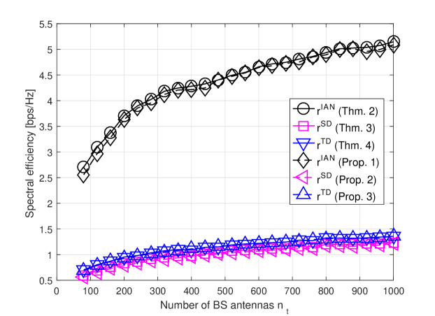
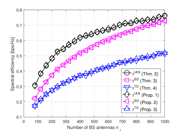
Figure 1: Finite vs. asymptotic analysis, weak interference, $n_{u}=40$, ${\rm SNR}=0$ dB.

    Figure 2: Finite vs. asymptotic analysis, moderate interference, $n_{u}=40$, ${\rm SNR}=0$ dB.

IV-B Asymptotic SE Comparison

We now compare the asymptotic SEs of the schemes detailed in Section III to the corresponding rates achievable using separate decoding with matched filtering and with MMSE filtering, computed via (4), where the SINR is computed using [6, Thm. 3], by averaging over all generated channel realizations. Here, the number of BS antennas is $n_{t}\!=\!800$, and the number of UTs in each cell is $n_{u}\!=\!80$. The achievable average ergodic rate of the time-division scheme is computed assuming optimal time partition, namely, via Corollary 1. Since time division can be considered as a form of cooperation between the cells, we compute the SE of the optimized scheme twice: once with optimal time division, via Corollary 2, and once with no time division, by maximizing the SE in Theorem 5 with $n_{p}=1$. To evaluate the SE versus SNR, $1/\sigma_{W}^{2}$, we fix the number of symbols used for channel estimation to $\tau_{p}=100$, and let the SNR vary from $-30$ dB to $30$ dB.

The results for the weak interference, moderate interference, and strong interference settings the are depicted in Figs. 4, 4, and 6, respectively. As expected, the optimized scheme obtains the highest SE in each setting over the entire SNR range, providing an indication on the true fundamental limits of massive MIMO systems. Furthermore, we observe in Fig. 4 that in the weak interference setting, although both the rates of Theorem 2 and [6, Thm. 3] are computed assuming that intercell interference is treated as noise, the achievable average ergodic rates of Theorem 2 are higher, with gains of $2.2$ bps/Hz and $0.45$ bps/Hz compared to matched filtering and MMSE filtering, respectively, at high SNRs, indicating that the SE of massive MIMO networks can be improved by allowing the BSs to perform joint decoding. We emphasize that an average ergodic rate gain of $0.45$ bps/Hz is translated into an overall ergodic rate gain of over $100$ bps/Hz in a cell with over $n_{u}=220$ UTs. Additionally, the SE of treating interference as noise coincides with that of the optimized scheme, which settles with the known theoretical result that for the two-user Gaussian interference, treating interference as noise is optimal in the weak interference regime [10, Ch. 6.4.3]. Furthermore, as was also noted in the illustrative example in Subsection III-E, in high SNRs, the performance of treating interference as noise is larger by a factor of approximately $n_{c}=5$ compared to simultaneous decoding and time division.

In the strong interference scenario, we observe in Fig. 6 that the optimized scheme as well as simultaneous decoding achieve an average ergodic rate of $0.55$ bps/Hz, while separate decoding results in negligible achievable rates, again, in agreement with the fact that simultaneous decoding is optimal in the strong interference regime for the two-user Gaussian interference channel, [10, Ch. 6.4.2]. Consequently, the fundamental limits of such channels are substantially higher than those achieved using standard separate linear decoding and treating interference as noise.

For the moderate interference setting, none of the schemes 1-3 achieves the performance of the optimized scheme, and thus there is a clear gain in combining these schemes using the optimized scheme of Subsection III-F. This gain follows since in this case, the received signal at each BS is impaired by notable intercell interference from some cells, and is hardly effected by the interference caused by other cells. Consequently, in this scenario, the fact that the optimized scheme allows treating the intercell interference caused by each cell differently is beneficial. For the weak interference and strong interference settings, whose results are depicted in Figs. 4 and 6, respectively, the optimized scheme does not utilize time-division, i.e., $n_{p}=1$ and $\{\zeta_{q}\}_{q=1}^{n_{p}}=\{1\}$. However, for the moderate interference setting, for which some of the intercell interference is neither too weak nor too dominant, it is observed in Fig. 4 that utilizing time-division is beneficial. In particular, the optimized scheme here divides the transmission phase into $n_{p}=2$ intervals. The first interval, which is utilized by $3$ cells, consists of $\zeta_{1}\approx 0.65$ of the transmission phase, while the remaining two cells utilize the rest of the transmission phase. Using this assignment, in high SNRs, the optimized scheme obtains a SE which is higher by $0.04$ bps/Hz compared to treating interference as noise when combining all three schemes, and by $0.018$ when combining only the decoding schemes 1-2, illustrating the benefit of combining time division. We also note that for all schemes, the achievable rates hardly vary with SNR at high SNRs, settling with the observation in [3, Sec. IV].

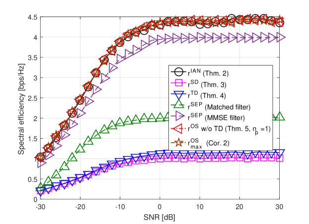
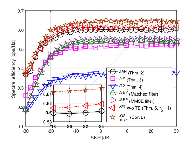
Figure 3: SE vs. SNR, weak interference.

    Figure 4: SE vs. SNR, moderate interference.

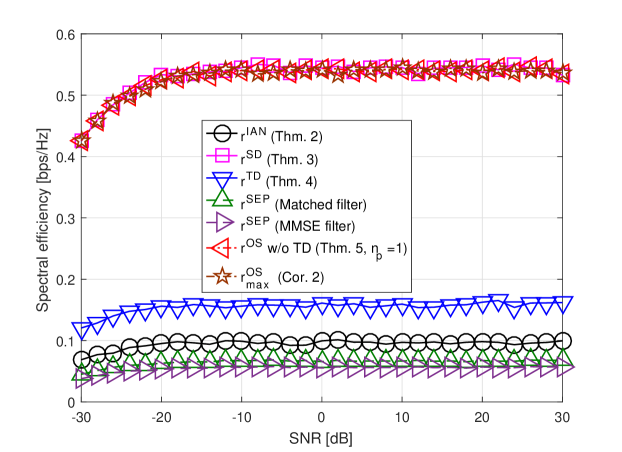
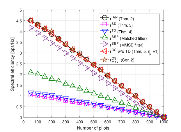
Figure 5: SE vs. SNR, strong interference.

    Figure 6: SE vs. number of pilots, weak interference.

Next, we numerically evaluate the dependence of the asymptotic SE on the number of pilot symbols. The purpose of this study is to check whether increasing $\tau_{p}$, which increases the channel estimation accuracy at the cost of reducing the portion of the coherence interval used for data transmission, is beneficial in terms of SE. It is emphasized that increasing $\tau_{p}$ can also contribute to reducing the effect of pilot contamination by supporting different pilot reuse factors [4]. However, to maintain consistency with the model used throughout the paper, in the following study we keep the pilot reuse factor to one, i.e., the same pilots are used in all the cells. In Fig. 6 we depict the SE versus the number of pilot symbols $\tau_{p}$ at SNR of $0$ dB for the weak interference setting. Observing Fig. 6, we note that, since the coherence duration is finite, for all the considered schemes, increasing the number of pilots linearly decreases the SE. A similar behavior was observed with the moderate interference and strong interference settings. We also note that the ratios between the SEs of the different schemes noted in Fig. 4 for $\tau_{p}=100$, is approximately maintained also for larger values of $\tau_{p}$.

In our last simulations study, we numerically evaluate how the SE of each of the considered schemes depends on the level of the intercell interference in practical massive MIMO setups. To that aim, we consider an area of one square kilometer, in which $n_{c}=5$ are placed such the cell of index $k=1$ is located in the center of the grid, and the rest of the BSs are located at equally spaced points on a circle with radius of $300$ meters. Here, $C_{k,l,m}$ represents the distance from the $m$-th UT of the $l$-th cell to the $k$-th BS. The location of each UT is uniformly distributed over the considered area. Each UT is associated to a BS based on the following rule: For a fixed $p\in[0,1]$, the UT is assigned with probability $p$ to the nearest BS, and with equal probability of $\frac{1-p}{4}$ to either of the other BSs. Such assignments can arise when the UT-cell association rule accounts for additional objectives, aside from the standard reference signal received power, see, e.g., [9]. An illustration of a realization of such a network with $n_{u}=10$ UTs and $p=0.8$ is depicted in Fig. 8. It is noted that as $p$ increases, it is more likely that each UT is associated with its nearest BS, thus the intercell interference becomes less dominant. Consequently, by letting $p$ vary from $0$ to $1$, we are able to control the level of intercell interference in the network.

In Fig. 8 we depict the SEs of the considered schemes versus $p$ for SNR of $0$ dB. Observing Fig. 8 we note that, as expected, for all values of $p$, the optimized scheme of Subsection III-F achieves the best performance. In particular, for small values of $p$, its performance coincides with that of simultaneous decoding, as the intercell interference is dominant. However, as $p$ increases, the effect of intercell interference is reduced, and treating interference as noise becomes optimal. Furthermore, it is illustrated that the standard approach of separate linear decoding achieves poor SE for most intercell interference levels, and is able to provide reasonable performance only for $p\geq 0.9$, namely, only when each UT is associated with its nearest BS with very high probability.

The results presented in this section demonstrate the potential benefits in terms of SE of properly acknowledging the nature of massive MIMO systems as interfering MACs. Furthermore, our results indicate the fundamental performance limits of such channels, and how far the conventional approach for massive MIMO systems is from capturing these characteristics.

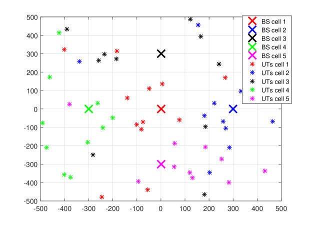
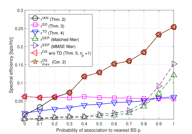
Figure 7: Network layout with $n_{u}=10$ and $p=0.8$.

    Figure 8: SE versus probability of association to nearest BS.

The results presented in this section demonstrate the potential benefits in terms of SE of properly acknowledging the nature of massive MIMO systems as interfering MACs. Furthermore, our results indicate the fundamental performance limits of such channels, and how far the conventional approach for massive MIMO systems is from capturing these characteristics.

V Conclusions

In this paper we studied the SE of uplink massive MIMO systems when the BSs are allowed to jointly decode the received signals. We characterized the achievable average ergodic rates of three schemes for handling the intercell interference, in both the finite and asymptotic antenna regimes, and studied a method which combines these approaches for handling the intercell interference, aimed at maximizing the SE. Simulation results demonstrate the gains obtained by allowing the BSs to perform joint decoding, and indicate that in some scenarios, the standard approach of separate linear decoding fails to capture the fundamental performance limits of massive MIMO systems, especially when the interference is dominant. The proposed analysis gives rise to a multitude of research paths, including the study of the SE with joint decoding under different system models, as well as the analysis and the derivation of network decoding schemes in presence of additional design objectives.

-A Proof of Lemma 1

In order to obtain the MMSE estimate of ${{\bf G}}_{k,l}$, we let $\tilde{{\bf S}}_{p}$ be the $\tau_{p}\times\tau_{p}$ unitary matrix (up to a fixed scaling constant) obtained from the full basis expansion of $\tilde{{\bf S}}$. Since $\tilde{{\bf S}}_{p}$ is deterministic and non-singular, it holds that the MMSE estimate satisfies

$$\hat{{{\bf G}}}_{k,l} =\mathcal{E}\left\{{{\bf G}}_{k,l}|{{\bf Y}}_{k},\{{{\bf D}}_{k,l}\}\right\}=\mathcal{E}\left\{{{\bf G}}_{k,l}|{{\bf Y}}_{k}\tilde{{\bf S}}_{p}^{H},\{{{\bf D}}_{k,l}\}\right\}$$

$$\stackrel{{\scriptstyle(a)}}{{=}}\mathcal{E}\left\{{{\bf G}}_{k,l}|{{\bf Y}}_{k}\tilde{{\bf S}}^{H},\{{{\bf D}}_{k,l}\}\right\},\vspace{-0.2cm}$$

where $(a)$ follows since, due the orthogonality of $\tilde{{\bf S}}_{p}$, the rows of ${{\bf Y}}_{k}\tilde{{\bf S}}_{p}^{H}$ which do not belong to ${{\bf Y}}_{k}\tilde{{\bf S}}^{H}$ contain only noise which, given $\{{{\bf D}}_{k,l}\}$, is independent of ${{\bf Y}}_{k}\tilde{{\bf S}}^{H}$, and $\{{{\bf G}}_{k,l}\}$. In particular, ${{\bf Y}}_{k}\tilde{{\bf S}}^{H}$ is a sufficient statistics of ${{\bf G}}_{k,l}$ from ${{\bf Y}}_{k}$ given $\{{{\bf D}}_{k,l}\}$ [30, Ch. 2.9].

Next, we note that by (6) it holds that ${{\bf Y}}_{k}\tilde{{\bf S}}^{H}=\tau_{p}\sum\limits_{l=1}^{n_{c}}{{\bf G}}_{k,l}+{{\bf W}}_{k}\tilde{{\bf S}}^{H}$. Thus, given $\{{{\bf D}}_{k,l}\}$, the entries of ${{\bf Y}}_{k}\tilde{{\bf S}}^{H}$ are mutually independent, and each entry of $\hat{{{\bf G}}}_{k,l}$ can be independently estimated from its corresponding entry of ${{\bf Y}}_{k}\tilde{{\bf S}}^{H}$. Since, given $\{{{\bf D}}_{k,l}\}$, ${{\bf Y}}_{k}\tilde{{\bf S}}^{H}$ and ${{\bf G}}_{k,l}$ are jointly Gaussian, the MMSE estimate of each entry is linear. Using the definition of ${{\bf B}}_{k,l}$ in (7), it can be shown that $\hat{{{\bf G}}}_{k,l}$ is given by

$$\hat{{{\bf G}}}_{k,l}={{\bf Y}}_{k}{{\bf S}}^{H}\tau_{p}^{-1}{{\bf B}}_{k,l},$$ (-A.1)

thus proving (8). Next, we study the statistical characterization of $\hat{{{\bf G}}}_{k,l}$. Note that by (-A.1),

$$\hat{{{\bf G}}}_{k,l} \stackrel{{\scriptstyle(a)}}{{=}}\left(\sum\limits_{l^{\prime}=1}^{n_{c}}{{\bf G}}_{k,l^{\prime}}{{\bf S}}+{{\bf W}}_{k}\right){{\bf S}}^{H}\tau_{p}^{-1}{{\bf B}}_{k,l}$$

$$\stackrel{{\scriptstyle(b)}}{{=}}\left(\sum\limits_{l^{\prime}=1}^{n_{c}}{{\bf H}}_{k,l^{\prime}}{{\bf D}}_{k,l^{\prime}}\right){{\bf B}}_{k,l}+\tau_{p}^{-1}{{\bf W}}_{k}{{\bf S}}^{H}{{\bf B}}_{k,l},$$ (-A.2)

where $(a)$ follows from the expression for ${{\bf Y}}_{k}$ in (6), and $(b)$ follows since ${{\bf G}}_{k,l}={{\bf H}}_{k,l}{{\bf D}}_{k,l}$ and ${{\bf S}}{{\bf S}}^{H}=\tau_{p}{{\bf I}}_{n_{u}}$. Since the entries of ${{\bf W}}_{k}$ are i.i.d. zero-mean Gaussian RVs with variance $\sigma_{W}^{2}$, the fact that ${{\bf S}}{{\bf S}}^{H}=\tau_{p}{{\bf I}}_{n_{u}}$ implies that the entries of the matrix ${{\bf W}}_{k}{{\bf S}}^{H}$ are i.i.d. zero-mean Gaussian RVs with variance $\sigma_{W}^{2}\tau_{p}$. Consequently, for a given realization $\{{{\bf D}}_{k,l}=\bar{{\bf D}}_{k,l}\}$ with diagonal coefficients $\{D_{k,l,m}=d_{k,l,m}\}$, we have that the entries of the diagonal matrix ${{\bf B}}_{k,l}$ are given by the deterministic values $\left({{\bf B}}_{k,l}\right)_{m,m}=\frac{\tau_{p}d_{k,l,m}^{2}}{\sigma_{W}^{2}+\tau_{p}\sum\limits_{l^{\prime}=1}^{n_{c}}d_{k,l^{\prime},m}^{2}}\triangleq\left(\bar{{\bf B}}_{k,l}\right)_{m,m}$. It thus follows from (-A.2) that the entries of $\hat{{{\bf G}}}_{k,l}$ are zero-mean mutually independent Gaussian RVs with variance $\mathcal{E}\Big{\{}\big{|}\big{(}\hat{{{\bf G}}}_{k,l}\big{)}_{m_{1},m_{2}}\big{|}^{2}\Big{|}\{{{\bf D}}_{k,l}\!=\!\bar{{\bf D}}_{k,l}\}\Big{\}}=\frac{\tau_{p}d_{k,l,m_{2}}^{2}}{\sigma_{W}^{2}+\tau_{p}\sum\limits_{l^{\prime}=1}^{n_{c}}d_{k,l^{\prime},m_{2}}^{2}}d_{k,l,m_{2}}^{2}=\left(\bar{{\bf B}}_{k,l}\right)_{m_{2},m_{2}}\left(\bar{{\bf D}}_{k,l}\right)_{m_{2},m_{2}}^{2}$. Accordingly, the conditional distribution of any set of entries from $\hat{{{\bf G}}}_{k,l}$ given $\{{{\bf D}}_{k,l}=\bar{{\bf D}}_{k,l}\}$ is identical to the conditional distribution of the corresponding set of entries from ${\bf M}{{\bf B}}_{k,l}^{1/2}{{\bf D}}_{k,l}$ given $\{{{\bf D}}_{k,l}=\bar{{\bf D}}_{k,l}\}$, recalling that ${\bf M}$ is a zero-mean Gaussian random matrix with i.i.d. unit variance entries independent of $\{{{\bf D}}_{k,l}\}_{l\in\mathcal{N}_{c}}$. It thus follows from the law of total probability [27, Ch. 8.2] that $\hat{{{\bf G}}}_{k,l}\stackrel{{\scriptstyle d}}{{=}}{\bf M}{{\bf B}}_{k,l}^{1/2}{{\bf D}}_{k,l}$. The proof that $\tilde{{{\bf G}}}_{k,l}\stackrel{{\scriptstyle d}}{{=}}{\bf M}\left({{\bf I}}_{n_{u}}-{{\bf B}}_{k,l}\right)^{1/2}{{\bf D}}_{k,l}$ is obtained using similar arguments and is thus omitted for brevity. ∎

-B Proof of Proposition 1

To prove the proposition, we first formulate the achievable ergodic sum-rate for the $k$-th BS using the covariance matrix of ${{\bf v}}^{\rm IAN}_{k}[i]$ conditioned on $\hat{{{\bf G}}}_{k,k}$ and $\{{{\bf D}}_{k,l}\}$, denoted ${\bf C}_{{{\bf v}}^{\rm IAN}_{k}|\hat{{{\bf G}}}_{k,k},\{{{\bf D}}_{k,l}\}}$. Then, we obtain an achievable ergodic sum-rate which depends on the covariance matrix of ${{{\bf v}}}^{\rm IAN}_{k}[i]$ conditioned only on $\{{{\bf D}}_{k,l}\}$, denoted ${\bf C}_{{{{\bf v}}}^{\rm IAN}_{k}|\{{{\bf D}}_{k,l}\}}$. Finally, we prove that the resulting achievable ergodic sum-rate yields the achievable average ergodic rate given in (13).

Let us first consider the achievable ergodic sum-rate of the MAC whose input-output relationship is given in (10) for a fixed $k\in\mathcal{N}_{c}$. During data transmission, the $k$-th BS knows the attenuation coefficients $\{{{\bf D}}_{k,l}\}$ and the estimated channel, $\hat{{{\bf G}}}_{k,k}$. Conditioned on these RVs, the estimation error $\tilde{{{\bf G}}}_{k,k}$ is zero-mean, since, by the law of total expectation [27, Ch. 7.4], $\mathcal{E}\left\{\tilde{{{\bf G}}}_{k,k}|\hat{{{\bf G}}}_{k,k},\{{{\bf D}}_{k,l}\}\right\}=\mathcal{E}\left\{\mathcal{E}\left\{{{{\bf G}}}_{k,k}|\hat{{{\bf G}}}_{k,k},{{\bf Y}}_{k},\{{{\bf D}}_{k,l}\right\}|\hat{{{\bf G}}}_{k,k},\{{{\bf D}}_{k,l}\}\right\}-\hat{{{\bf G}}}_{k,k}$, and thus,

$$\mathcal{E}\left\{\tilde{{{\bf G}}}_{k,k}|\hat{{{\bf G}}}_{k,k},\{{{\bf D}}_{k,l}\}\right\}\stackrel{{\scriptstyle(a)}}{{=}}\mathcal{E}\left\{\hat{{{\bf G}}}_{k,k}|\hat{{{\bf G}}}_{k,k},\{{{\bf D}}_{k,l}\}\right\}-\hat{{{\bf G}}}_{k,k}=0,\vspace{-0.2cm}$$ (-B.1)

where $(a)$ follows since $\hat{{{\bf G}}}_{k,k}$ is the MMSE estimate of ${{{\bf G}}}_{k,k}$ given ${{\bf Y}}_{k}$, $\{{{\bf D}}_{k,l}\}$, Consequently, the equivalent noise ${{\bf v}}^{\rm IAN}_{k}[i]$ is orthogonal to ${{\bf x}}_{k}[i]$, thus (10) represents a MAC with an additive uncorrelated noise ${{\bf v}}^{\rm IAN}_{k}[i]$ and a known channel matrix $\hat{{{\bf G}}}_{k,k}$. Since the worst-case additive uncorrelated noise distribution is Gaussian [13, Thm. 1], the achievable ergodic sum-rate of the MAC (10) with Gaussian ${{\bf v}}^{\rm IAN}_{k}[i]$ is also achievable with any other distribution of ${{\bf v}}^{\rm IAN}_{k}[i]$.

By letting the codelength span a sufficiently large number of realizations of $\{{{\bf D}}_{k,l}\}$ and $\{{{\bf H}}_{k,l}\}$, noting that the BS knows the channel attenuations and the MMSE estimate of the channel, the following ergodic sum-rate is achievable for the MAC (10) [10, Ch. 23.5]:

$$\sum\limits_{m=1}^{n_{u}}\!r_{k,m} =I\left({{\bf x}}_{k};{{\bf y}}_{k}|\hat{{{\bf G}}}_{k,k},\{{{\bf D}}_{k,l}\}\right)$$

$$\stackrel{{\scriptstyle(a)}}{{\geq}}\mathcal{E}\left\{\log\left|{{\bf I}}_{n_{t}}\!+\!\hat{{{\bf G}}}_{k,k}\hat{{{\bf G}}}_{k,k}^{H}{\bf C}_{{{\bf v}}^{\rm IAN}_{k}|\hat{{{\bf G}}}_{k,k},\{{{\bf D}}_{k,l}\}}^{-1}\right|\right\}$$

$$=\mathcal{E}\left\{\log\left|{\bf C}_{{{\bf v}}^{\rm IAN}_{k}|\hat{{{\bf G}}}_{k,k},\{{{\bf D}}_{k,l}\}}\!+\!\hat{{{\bf G}}}_{k,k}\hat{{{\bf G}}}_{k,k}^{H}\right|\right\}$$

$$-\mathcal{E}\left\{\log\left|{\bf C}_{{{\bf v}}^{\rm IAN}_{k}|\hat{{{\bf G}}}_{k,k},\{{{\bf D}}_{k,l}\}}\right|\right\},$$ (-B.2)

where $(a)$ follows by computing the mutual information for Gaussian additive uncorrelated noise ${{\bf v}}^{\rm IAN}_{k}[i]$ [10, Ch. 9.1], as the worst-case additive noise is Gaussian.

Next, we explicitly express the matrix ${\bf C}_{{{\bf v}}^{\rm IAN}_{k}|\hat{{{\bf G}}}_{k,k},\{{{\bf D}}_{k,l}\}}$. Note that from (7) and (8), $\hat{{{\bf G}}}_{k,l}=\hat{{{\bf G}}}_{k,k}{{\bf D}}_{k,k}^{-2}{{\bf D}}_{k,l}^{2}$, and therefore, ${{{\bf v}}}^{\rm IAN}_{k}[i]=\sum\limits_{l=1}^{n_{c}}\tilde{{{\bf G}}}_{k,l}{{\bf x}}_{l}[i]+\hat{{{\bf G}}}_{k,k}{{\bf D}}_{k,k}^{-2}\sum\limits_{l=1,l\neq k}^{n_{c}}{{\bf D}}_{k,l}^{2}{{\bf x}}_{l}[i]+{{\bf w}}_{k}[i]$. As $\{\tilde{{{\bf G}}}_{k,l}\}$ and $\hat{{{\bf G}}}_{k,k}$ are jointly Gaussian and uncorrelated given $\{{{\bf D}}_{k,l}\}$, then, ${\bf C}_{{{{\bf v}}}^{\rm IAN}_{k}|\hat{{{\bf G}}}_{k,k},\{{{\bf D}}_{k,l}\}}=\sum\limits_{l=1}^{n_{c}}\mathcal{E}\left\{\tilde{{{\bf G}}}_{k,l}\tilde{{{\bf G}}}_{k,l}^{H}|\{{{\bf D}}_{k,l}\}\right\}+\hat{{{\bf G}}}_{k,k}{{\bf D}}_{k,k}^{-4}\sum\limits_{l=1,l\neq k}^{n_{c}}{{\bf D}}_{k,l}^{4}\hat{{{\bf G}}}_{k,k}^{H}+\sigma_{W}^{2}{{\bf I}}_{n_{t}}$, which yields

$${\bf C}_{{{{\bf v}}}^{\rm IAN}_{k}|\hat{{{\bf G}}}_{k,k},\{{{\bf D}}_{k,l}\}} \stackrel{{\scriptstyle(a)}}{{=}}T_{k}\cdot{{\bf I}}_{n_{t}}$$

$$+\hat{{{\bf G}}}_{k,k}{{\bf D}}_{k,k}^{-4}\sum\limits_{l=1,l\neq k}^{n_{c}}{{\bf D}}_{k,l}^{4}\hat{{{\bf G}}}_{k,k}^{H},\vspace{-0.2cm}$$ (-B.3)

where $(a)$ follows from Lemma 1, as for any ${\bf Q}$, $\mathcal{E}\{{\bf M}{\bf Q}{\bf M}^{H}\}={\rm Tr}\left({\bf Q}\right){{\bf I}}_{n_{t}}$ [29, Sec. III-B].

Substituting (-B.3) into (-B.2), recalling that $\hat{{{\bf G}}}_{k,k}\stackrel{{\scriptstyle d}}{{=}}{\bf M}{{\bf B}}_{k,k}^{1/2}{{\bf D}}_{k,k}$, where ${{\bf B}}_{k,k}$ and ${{\bf D}}_{k,k}$ are diagonal matrices with strictly positive diagonal entries, results in

$$\sum\limits_{m=1}^{n_{u}}\!r_{k,m} \geq\mathcal{E}\left\{\log\left|{{\bf I}}_{n_{t}}+{\bf M}{{\bf Q}}^{\rm Net}_{k}{\bf M}^{H}\right|\right\}$$

$$-\mathcal{E}\left\{\log\left|{{\bf I}}_{n_{t}}+{\bf M}{{\bf Q}}^{\rm Int}_{k}{\bf M}^{H}\right|\right\},$$ (-B.4)

where ${{\bf Q}}^{\rm Net}_{k},{{\bf Q}}^{\rm Int}_{k}$ are defined in (12). This proves that $r^{\rm IAN}_{n_{t}}$ given in (13) is achievable. ∎

-C Proof of Theorem 2

We prove the theorem by applying Theorem 1 to characterize (13) in the limit $n_{t}\rightarrow\infty$ with $\frac{n_{u}}{n_{t}}=\kappa$. To that aim, we first show that the conditions of Theorem 1 are satisfied, and then we apply Theorem 1 to obtain (15). We now explicitly derive $\mathop{\lim}\limits_{{n_{t}\rightarrow\infty}}\mathcal{E}\left\{\frac{1}{n_{t}}\log\left|{{\bf I}}_{n_{t}}+{\bf M}{{\bf Q}}^{\rm Net}_{k}{\bf M}^{H}\right|\right\}$; the derivation of this limit with ${{\bf Q}}^{\rm Net}_{k}$ replaced by ${{\bf Q}}^{\rm Int}_{k}$ is similar and thus omitted for brevity.

As the entries of ${\bf M}$ are i.i.d. unit variance RVs independent of ${{\bf Q}}^{\rm Net}_{k}$, the matrix ${\bf M}{{\bf Q}}^{\rm Net}_{k}{\bf M}^{H}=\frac{1}{n_{t}}{\bf M}\big{(}n_{t}\cdot{{\bf Q}}^{\rm Net}_{k}\big{)}{\bf M}^{H}$ satisfies the conditions of Theorem 1 when the empirical eigenvalue distribution of $n_{t}\cdot{{\bf Q}}^{\rm Net}_{k}$ converges to a non-random limit almost surely. Since $n_{t}\cdot{{\bf Q}}^{\rm Net}_{k}$ is a diagonal matrix, its eigenvalues are given by its diagonal entries $\left(n_{t}\!\cdot\!{{\bf Q}}^{\rm Net}_{k}\right)_{m,m}=\frac{B_{k,k,m}D_{k,k,m}^{-2}\sum\limits_{l=1}^{n_{c}}D_{k,l,m}^{4}}{\kappa\sum\limits_{l=1}^{n_{c}}\!\big{(}\!\frac{1}{n_{u}}\!\sum\limits_{m^{\prime}=1}^{n_{u}}\!\left(1\!-\!B_{k,l,m^{\prime}}\right)D_{k,l,m^{\prime}}^{2}\!\big{)}\!+\!\frac{1}{n_{t}}\sigma_{W}^{2}}$, for $m\in\mathcal{N}_{u}$. From (7), it follows that for any $k,l\in\mathcal{N}_{c}$ the RVs $\big{\{}\left(1-B_{k,l,m^{\prime}}\right)D_{k,l,m^{\prime}}^{2}\big{\}}_{m^{\prime}\in\mathcal{N}_{u}}$ are i.i.d., and thus, by the strong law of large numbers [28, Ch. 2.4], $\frac{1}{n_{u}}\sum\limits_{m^{\prime}=1}^{n_{u}}\left(1-B_{k,l,m^{\prime}}\right)D_{k,l,m^{\prime}}^{2}$ converges almost surely to $\mathcal{E}\{\left(1-B_{k,l,1}\right)D_{k,l,1}^{2}\}$. Consequently, it follows from [31, Ch. 20.6] that for sufficiently large $n_{t}$ with fixed $\frac{n_{u}}{n_{t}}=\kappa$, the distribution of the eigenvalues of $n_{t}\cdot{{\bf Q}}^{\rm Net}_{k}$ approaches the distribution of the set of i.i.d. RVs $\Big{\{}\frac{B_{k,k,m}D_{k,k,m}^{-2}\sum\limits_{l=1}^{n_{c}}D_{k,l,m}^{4}}{\kappa\sum\limits_{l=1}^{n_{c}}\mathcal{E}\{\left(1-B_{k,l,1}\right)D_{k,l,1}^{2}\}}\Big{\}}_{m\in\mathcal{N}_{u}}$. It therefore follows from [28, Thm. 2.4.7] that the empirical CDF of the eigenvalues of $n_{t}\cdot{{\bf Q}}^{\rm Net}_{k}$ converges almost surely to the non-random CDF of the random variable $A^{\rm Net}_{k}$ defined in (14), and that the random matrix ${\bf M}{{\bf Q}}^{\rm Net}_{k}{\bf M}^{H}$ satisfies the conditions of Theorem 1. Consequently, in the massive MIMO regime, the achievable average ergodic rate in (13) can be written as in (15). ∎

-D Proof of Proposition 2

When each BS decodes the messages of all UTs in the network, the input-output relationship (17) represents a set of $n_{c}$ MACs with $n_{c}\cdot n_{u}$ transmitters. Thus, letting the codelength span a sufficiently large number of realizations of $\{{{\bf D}}_{k,l}\}$ and $\{{{\bf H}}_{k,l}\}$, as the BS knows the attenuation coefficients and the MMSE channel estimate, every sum-rate which satisfies

$$\sum\limits_{l=1}^{n_{c}}\sum\limits_{m=1}^{n_{u}}\!r_{l,m}\!\leq\!I\!\left({{\bf x}}_{1},{{\bf x}}_{2},\ldots,{{\bf x}}_{n_{c}};{{{\bf y}}}_{k}|\hat{{{\bf G}}}_{k,k},\{{{\bf D}}_{k,l}\}\right),$$ (-D.1)

$\forall k\in\mathcal{N}_{c},$ is an achievable ergodic sum-rate [10, Ch. 23.5].

Let ${\bf C}_{{{{\bf v}}}^{\rm SD}_{k}|\{{{\bf D}}_{k,l}\}}$ and ${\bf C}_{{{{\bf v}}}^{\rm SD}_{k}|\hat{{{\bf G}}}_{k,k},\{{{\bf D}}_{k,l}\}}$ be the covariance matrices of ${{{\bf v}}}^{\rm SD}_{k}[i]$ conditioned on $\{{{\bf D}}_{k,l}\}$ and on $\hat{{{\bf G}}}_{k,k},\{{{\bf D}}_{k,l}\}$, respectively. Repeating the arguments in (-B.1), we have that the equivalent noise ${{\bf v}}^{\rm SD}_{k}[i]=\sum\limits_{l=1}^{n_{c}}\tilde{{{\bf G}}}_{k,l}{{\bf x}}_{l}[i]+{{\bf w}}_{k}[i]$ is orthogonal to ${{\bf x}}_{l}[i]$ for every $k,l\in\mathcal{N}_{c}$. Since the worst-case additive uncorrelated noise distribution is Gaussian [13, Thm. 1], by computing the mutual information (-D.1) with Gaussian ${{\bf v}}^{\rm SD}_{k}[i]$ we have that [10, Ch. 9.1] $I\left({{\bf x}}_{1},{{\bf x}}_{2},\ldots,{{\bf x}}_{n_{c}};{{{\bf y}}}_{k}|\hat{{{\bf G}}}_{k,k},\{{{\bf D}}_{k,l}\}\right)\geq\mathcal{E}\left\{\log\left|{{\bf I}}_{n_{t}}+\hat{{{\bf G}}}_{k,k}{{\bf D}}_{k,k}^{-4}\sum\limits_{l=1}^{n_{c}}{{\bf D}}_{k,l}^{4}\hat{{{\bf G}}}_{k,k}^{H}{\bf C}_{{{{\bf v}}}^{\rm SD}_{k}|\hat{{{\bf G}}}_{k,k}\{{{\bf D}}_{k,l}\}}^{-1}\right|\right\}$. As $\{{{\bf D}}_{k,l}\}$ are diagonal matrices with strictly positive diagonal entries, and since given $\{{{\bf D}}_{k,l}\}$, each MMSE estimate $\hat{{{\bf G}}}_{k,l}$ is jointly Gaussian and uncorrelated with the estimation error $\tilde{{{\bf G}}}_{k,l}$, it follows that ${{{\bf v}}}^{\rm SD}_{k}[i]$ is independent of $\hat{{{\bf G}}}_{k,k}$ given $\{{{\bf D}}_{k,l}\}$, and thus

$$I\left({{\bf x}}_{1},{{\bf x}}_{2},\ldots,{{\bf x}}_{n_{c}};{{{\bf y}}}_{k}|\hat{{{\bf G}}}_{k,k},\{{{\bf D}}_{k,l}\}\right)\!\geq\!\mathcal{E}\left\{\log\left|{{\bf I}}_{n_{t}}\!+\!\hat{{{\bf G}}}_{k,k}{{\bf D}}_{k,k}^{-4}\sum\limits_{l=1}^{n_{c}}{{\bf D}}_{k,l}^{4}\hat{{{\bf G}}}_{k,k}^{H}{\bf C}_{{{{\bf v}}}^{\rm SD}_{k}|\{{{\bf D}}_{k,l}\}}^{-1}\right|\right\}.\vspace{-0.2cm}$$ (-D.2)

Next, repeating the arguments used in (-B.3) to compute ${\bf C}_{\tilde{{{\bf v}}}^{\rm IAN}_{k}|\{{{\bf D}}_{k,l}\}}$, we have that ${\bf C}_{{{{\bf v}}}^{\rm SD}_{k}|\{{{\bf D}}_{k,l}\}}=\sum\limits_{l=1}^{n_{c}}{\rm Tr}\left(\left({{\bf I}}_{n_{u}}\!-\!{{\bf B}}_{k,l}\right){{\bf D}}_{k,l}^{2}\right){{\bf I}}_{n_{t}}\!+\!\sigma_{W}^{2}{{\bf I}}_{n_{t}}=T_{k}^{-1}\cdot{{\bf I}}_{n_{t}}$. Consequently, from Lemma 1 and (12), we have that $\hat{{{\bf G}}}_{k,k}{{\bf D}}_{k,k}^{-4}\sum\limits_{l=1}^{n_{c}}{{\bf D}}_{k,l}^{4}\hat{{{\bf G}}}_{k,k}^{H}{\bf C}_{{{{\bf v}}}^{\rm SD}_{k}|\{{{\bf D}}_{k,l}\}}^{-1}\stackrel{{\scriptstyle d}}{{=}}{\bf M}{{\bf Q}}^{\rm Net}_{k}{\bf M}^{H}$, Combining this with (-D.2) yields

$$I\left({{\bf x}}_{1},{{\bf x}}_{2},\ldots,{{\bf x}}_{n_{c}};{{{\bf y}}}_{k}|\hat{{{\bf G}}}_{k,k},\{{{\bf D}}_{k,l}\}\right)\geq\mathcal{E}\left\{\log\left|{{\bf I}}_{n_{t}}+{\bf M}{{\bf Q}}^{\rm Net}_{k}{\bf M}^{H}\right|\right\}.\vspace{-0.2cm}$$ (-D.3)

It thus follows from (-D.1) and (-D.3) that $\mathop{\min}\limits_{k\in\mathcal{N}_{c}}\mathcal{E}\left\{\log\left|{{\bf I}}_{n_{t}}+{\bf M}{{\bf Q}}^{\rm Net}_{k}{\bf M}^{H}\right|\right\}$ is an achievable ergodic sum-rate for the MACs given by (17), and thus, $r^{\rm SD}_{n_{t}}$ given in (18) is an achievable average ergodic rate when the BSs decode the intercell interference, proving the proposition. ∎

-E Proof of Proposition 3

When the intercell interference is eliminated using time-division, the input-output relationship (21) represents a set of $n_{c}$ MACs, each with $n_{u}$ transmitters. Thus, letting the codelength span a sufficiently large number of realizations of the attenuation coefficients $\{{{\bf D}}_{k,l}\}$ and channel matrices $\{{{\bf H}}_{k,l}\}$, as the BS knows the attenuation coefficients and the MMSE channel estimate, the following ergodic sum-rate is achievable for the $k$-th MAC (21), $k\in\mathcal{N}_{c}$ [10, Ch. 23.5]:

$$\sum\limits_{m=1}^{n_{u}}\!r_{k,m}\!\leq\!I\!\left({{\bf x}}_{k};{{{\bf y}}}_{k}|\hat{{{\bf G}}}_{k,k},\{{{\bf D}}_{k,l}\}\right).\vspace{-0.2cm}$$ (-E.1)

Let ${\bf C}_{{{{\bf v}}}^{\rm TD}_{k}|\{{{\bf D}}_{k,l}\}}$ be the covariance matrices of ${{{\bf v}}}^{\rm TD}_{k}[i]$ conditioned on $\{{{\bf D}}_{k,l}\}$. Note that ${{\bf v}}^{\rm TD}_{k}=\tilde{{{\bf G}}}_{k,k}\zeta_{k}^{-\frac{1}{2}}{{\bf x}}_{k}[i]+{{\bf w}}_{k}[i]$ is independent of the MMSE estimate $\hat{{{\bf G}}}_{k,k}$ given $\{{{\bf D}}_{k,l}\}$, and orthogonal to ${{\bf x}}_{k}[i]$ for every $k\in\mathcal{N}_{c}$. Since the worst-case additive uncorrelated noise distribution is Gaussian [13, Thm. 1], by computing (-E.1) with Gaussian ${{\bf v}}^{\rm TD}_{k}[i]$ we have that [10, Ch. 9.1] $I\left({{\bf x}}_{k};{{{\bf y}}}_{k}|\hat{{{\bf G}}}_{k,k},\{{{\bf D}}_{k,l}\}\right)\geq\mathcal{E}\left\{\log\left|{{\bf I}}_{n_{t}}+\hat{{{\bf G}}}_{k,k}\hat{{{\bf G}}}_{k,k}^{H}{\bf C}_{{{{\bf v}}}^{\rm TD}_{k}|\{{{\bf D}}_{k,l}\}}^{-1}\right|\right\}$. Next, repeating the arguments used in (-B.3) to compute ${\bf C}_{\tilde{{{\bf v}}}^{\rm IAN}_{k}|\{{{\bf D}}_{k,l}\}}$, we have that ${\bf C}_{{{{\bf v}}}^{\rm TD}_{k}|\{{{\bf D}}_{k,l}\}}=\zeta_{k}^{-1}{\rm Tr}\left(\left({{\bf I}}_{n_{u}}\!-\!{{\bf B}}_{k,k}\right){{\bf D}}_{k,k}^{2}\right){{\bf I}}_{n_{t}}\!+\!\sigma_{W}^{2}{{\bf I}}_{n_{t}}$. Thus, from Lemma 1 and (22), $\zeta_{k}^{-1}\hat{{{\bf G}}}_{k,k}\hat{{{\bf G}}}_{k,k}^{H}{\bf C}_{{{{\bf v}}}^{\rm TD}_{k}|\{{{\bf D}}_{k,l}\}}^{-1}\stackrel{{\scriptstyle d}}{{=}}{\bf M}{{\bf Q}}^{\rm TD}_{k}\!\left(\zeta_{k}\right){\bf M}^{H}$. From (-E.1), we have that $\mathcal{E}\left\{\log\left|{{\bf I}}_{n_{t}}\!+\!{\bf M}{{\bf Q}}^{\rm TD}_{k}\!\left(\zeta_{k}\right){\bf M}^{H}\right|\right\}$ is an achievable ergodic sum-rate for the MAC whose input-output relationship is given in (21). As each MAC uses only $\zeta_{k}$ of the data transmission phase, the SE is given in (23), proving the proposition. ∎

-F Proof of Proposition 4

To prove the proposition, we first express the RVs $A^{\rm Net}_{k}$, $A^{\rm Int}_{k}$, and $A^{\rm TD}_{k}$, for the considered setup, and the corresponding SEs $r^{\rm IAN}$, $r^{\rm SD}$, and $r^{\rm TD}$. Then, we use these expressions to characterize the relationships between the asymptotic SEs when $y_{\max}\ll x_{\min}$ and when $x_{\max}\ll y_{\min}$.

First, we note that for the considered setup, the RVs $B_{k,l,m}$ defined in (7) are distributed via $B_{k,l,m}\stackrel{{\scriptstyle d}}{{=}}\frac{\tau_{p}X}{\sigma_{W}^{2}+\tau_{p}(X+Y)}$ for $k=l$ and $B_{k,l,m}\stackrel{{\scriptstyle d}}{{=}}\frac{\tau_{p}Y}{\sigma_{W}^{2}+\tau_{p}(X+Y)}$ for $k\neq l$, for each $m\in\mathcal{N}_{u}$. Consequently, by defining $\mu_{X,Y}\triangleq\mathcal{E}\big{\{}\frac{\sigma_{W}^{2}+\tau_{p}\cdot X\dot{Y}}{\sigma_{W}^{2}+\tau_{p}(X+Y)}\big{\}}\underset{\sigma_{W}^{2}\to 0}{=}\mathcal{E}\big{\{}\frac{X\cdot Y}{X+Y}\big{\}}$, for each $k=1,2$, $A^{\rm Net}_{k}$ defined in (14) satisfies $A^{\rm Net}_{k}=\frac{B_{k,k,1}D_{k,k,1}^{-2}(D_{k,1,1}^{4}+D_{k,2,1}^{4})}{\kappa\left(\mathcal{E}\{\left(1-B_{k,1,1}\right)D_{k,1,1}^{2}\}+\mathcal{E}\{\left(1-B_{k,2,1}\right)D_{k,2,1}^{2}\}\right)}$, and thus

$$A^{\rm Net}_{k}\stackrel{{\scriptstyle d}}{{=}} \frac{\tau_{p}}{\kappa\cdot\mu_{X,Y}}\frac{X^{2}+Y^{2}}{\sigma_{W}^{2}+\tau_{p}(X+Y)}$$

$$\stackrel{{\scriptstyle(a)}}{{=}}\frac{1}{\kappa\cdot\mu_{X,Y}}\frac{X^{2}+Y^{2}}{X+Y},\vspace{-0.2cm}$$ (-F.1)

where $(a)$ follows since $\sigma_{W}^{2}\rightarrow 0$. Similarly, the RVs $A^{\rm Int}_{k}$ and $A^{\rm TD}_{k}$ satisfy

$$A^{\rm Int}_{k}\stackrel{{\scriptstyle d}}{{=}}\frac{1}{\kappa\cdot\mu_{X,Y}}\frac{Y^{2}}{X+Y},\quad A^{\rm TD}_{k}\stackrel{{\scriptstyle d}}{{=}}\frac{1}{\kappa\cdot\mu_{X,Y}}\frac{X^{2}}{X+Y},$$ (-F.2)

for each $k=1,2$. It follows (-F.1)-(-F.2) that the distribution of the RVs $A^{\rm Net}_{k}$, $A^{\rm Int}_{k}$, and $A^{\rm TD}_{k}$ does not depend on $k$, and thus the asymptotic SEs in (15), (19), and (26), satisfy for any $k=1,2$

$$r^{\rm IAN} = \frac{\tau_{d}}{\tau_{c}\cdot\kappa}\!\left(\nu\left(A^{\rm Net}_{k},\kappa\right)\!-\!\nu\left(A^{\rm Int}_{k},\kappa\right)\right);$$ (-F.3a)

$$r^{\rm SD} = \frac{\tau_{d}}{2\tau_{c}\cdot\kappa}\nu\left(A^{\rm Net}_{k},\kappa\right);$$ (-F.3b)

$$r^{\rm TD} = \frac{\tau_{d}}{2\tau_{c}\cdot\kappa}\nu\left(A^{\rm TD}_{k},\kappa\right).\vspace{-0.2cm}$$ (-F.3c)

To characterize the relationship between $r^{\rm SD}$ and $r^{\rm IAN}$, we use the following lemma:

Lemma -F.1.

For an RV $A$ satisfying $\Pr\left(0\leq A<a_{\max}\right)=1$, if $\kappa\cdot\mathcal{E}\left\{\frac{\eta\cdot A}{1+\eta\cdot A}\right\}<\frac{1}{2}$, where $\eta\in(0,1]$ is given in Theorem 1, then $\nu\left(A,\kappa\right)\leq\kappa\cdot\log(1+a_{\max})+\log e\cdot\left(\kappa\cdot\frac{a_{\max}}{1+a_{\max}}\right)^{2}$.

Proof:

Note that $\eta\!=\!1\!-\!\kappa\cdot\mathcal{E}\left\{\frac{\eta\cdot A}{1+\eta\cdot A}\right\}$. For $\kappa\cdot\mathcal{E}\left\{\frac{\eta\cdot A}{1+\eta\cdot A}\right\}<\frac{1}{2}$, plugging this into (5) yields

$$\nu\left(A,\kappa\right)=\kappa\cdot\mathcal{E}\left\{\log(1\!+\!\eta\cdot A)\right\}\!+\!\log e$$

$$\qquad\cdot\left(-\kappa\cdot\mathcal{E}\left\{\frac{\eta\cdot A}{1\!+\!\eta\cdot A}\right\}-\log_{e}\left(1-\kappa\cdot\mathcal{E}\left\{\frac{\eta\cdot A}{1\!+\!\eta\cdot A}\right\}\right)\right)$$

$$\stackrel{{\scriptstyle(a)}}{{\leq}}\kappa\cdot\mathcal{E}\left\{\log(1\!+\!\eta\cdot A)\right\}\!+\!\log e\cdot\left(\!\kappa\cdot\mathcal{E}\left\{\frac{\eta\cdot A}{1\!+\!\eta\cdot A}\right\}\right)^{2}\!\!,\vspace{-0.2cm}$$ (-F.4)

where $(a)$ follows since for $\alpha\in[0,\frac{1}{2}]$, $-\alpha-\alpha^{2}\leq\log_{e}(1-\alpha)$. As $\frac{\alpha}{1+\alpha}$ and $\log(1+\alpha)$ are monotonically non-decreasing and $\eta\cdot A\leq a_{\max}$, (-F.4) proves the lemma. ∎

We can now prove that when $y_{\max}\ll x_{\min}$, $r^{\rm IAN}\approx 2r^{\rm SD}$. From (-F.3) we have that $r^{\rm IAN}=2\cdot r^{\rm SD}-\frac{\tau_{d}}{\tau_{c}\cdot\kappa}\nu\left(A^{\rm Int}_{k},\kappa\right)$. Next, we prove that $A^{\rm Int}_{k}$ satisfies the conditions of Lemma -F.1. note that $A^{\rm Int}_{k}\leq\frac{1}{\kappa\cdot\mu_{X,Y}}\frac{y_{\max}^{2}}{y_{\max}+x_{\min}}\triangleq a_{\max}$ with probability one, and thus $\kappa\cdot\mathcal{E}\left\{\frac{\eta\cdot A^{\rm Int}_{k}}{1+\eta\cdot A^{\rm Int}_{k}}\right\}\leq\kappa\cdot\frac{a_{\max}}{1+a_{\max}}$. Furthermore, since $Y\ll X$ with probability one, we have that $\mu_{X,Y}\approx\mathcal{E}\{Y\}$, and thus $a_{\max}\approx\frac{y_{\max}}{\kappa\cdot\mathcal{E}\{Y\}}\frac{y_{\max}}{x_{\min}}$. Consequently, since $y_{\max}\ll x_{\min}$ then $a_{\max}\approx 0$, and thus $\kappa\cdot\mathcal{E}\left\{\frac{\eta\cdot A^{\rm Int}_{k}}{1+\eta\cdot A^{\rm Int}_{k}}\right\}<\frac{1}{2}$. Thus, $A^{\rm Int}_{k}$ satisfies the conditions of Lemma -F.1, and therefore, $\nu\left(A^{\rm Int}_{k},\kappa\right)\leq\kappa\cdot\log(1+a_{\max})+\log e\cdot\left(\kappa\cdot\frac{a_{\max}}{1+a_{\max}}\right)^{2}\stackrel{{\scriptstyle(a)}}{{\approx}}0$, where $(a)$ follows since $a_{\max}$ tends to zero. Consequently, $r^{\rm IAN}\approx 2r^{\rm SD}$.

Lastly, we consider the case in which $x_{\max}\ll y_{\max}$. Here, we have that $X\ll Y$ with probability one. In this case it follows from (-F.1) and (-F.2) that for any $k=1,2$, the distribution of the RVs $A^{\rm Net}_{k}$ and $A^{\rm Int}_{k}$ approaches the distribution of the RV $\frac{Y}{\kappa\cdot\mu_{X,Y}}$. Consequently, by (-F.3), we have that $r^{\rm IAN}\approx 0$. Similarly, the distribution of $A^{\rm TD}_{k}$ approaches the distribution of the RV $\frac{1}{\kappa\cdot\mu_{X,Y}}\frac{X^{2}}{Y}$. Consequently, by (-F.3), $r^{\rm SD}\approx\frac{\tau_{d}}{2\tau_{c}\cdot\kappa}\nu\left(\frac{Y}{\kappa\cdot\mu_{X,Y}},\kappa\right)$, and $r^{\rm TD}\approx\frac{\tau_{d}}{2\tau_{c}\cdot\kappa}\nu\left(\frac{1}{\kappa\cdot\mu_{X,Y}}\frac{X^{2}}{Y}.\kappa\right)$, Now, by considering the same network in which the UTs of cell $k=1$ are allocated to to cell $k=2$ and vice versa, we have that the SE of treating interference as noise, which is strictly positive, is given by $\frac{\tau_{d}}{\tau_{c}\cdot\kappa}\big{(}\nu\left(\frac{Y}{\kappa\cdot\mu_{X,Y}},\kappa\right)\!-\!\nu\left(\frac{1}{\kappa\cdot\mu_{X,Y}}\frac{X^{2}}{Y}.\kappa\right)\big{)}>0$. Thus, $r^{\rm SD}>r^{\rm TD}$. ∎

-G Proof of Theorem 5

To prove the theorem, we first obtain the SE in the finite antenna regime, and then we let $n_{t}$ tend to infinity and use Theorem 1 to obtain (29). From the representation in (28), by treating ${{\bf v}}^{\rm OS}_{k}$ as noise and decoding the interference $\{{{\bf x}}_{l}\}_{l\in\mathcal{J}_{q}^{s},l\neq k}$, we have that ${{\bf y}}_{k}$ is the output of a MAC with $|\mathcal{J}_{q}^{s}|\cdot n_{u}$ transmitters. Consequently, by repeating the arguments in the proofs of Propositions 1-3, we have that for each cluster $\mathcal{J}_{q}^{s}$, every sum-rate with satisfies that

$$\sum\limits_{l\in\mathcal{J}_{q}^{s}}\sum\limits_{m=1}^{n_{u}}\!r_{l,m}\!\leq\!I\!\left(\{{{\bf x}}_{l}\}_{l\in\mathcal{J}_{q}^{s}};{{{\bf y}}}_{k}|\hat{{{\bf G}}}_{k,k},\{{{\bf D}}_{k,l}\}\right),$$ (-G.1)

$\forall k\in\mathcal{J}_{q}^{s}$, is an achievable ergodic sum-rate [10, Ch. 23.5].

$$I\!\left(\{{{\bf x}}_{l}\}_{l\in\mathcal{J}_{q}^{s}};{{{\bf y}}}_{k}|\hat{{{\bf G}}}_{k,k},\{{{\bf D}}_{k,l}\}\right)\geq\mathcal{E}\bigg{\{}\log\bigg{|}{{\bf I}}_{n_{t}}\!+\!\zeta_{q}^{-1}\hat{{{\bf G}}}_{k,k}{{\bf D}}_{k,k}^{-4}\sum\limits_{l\in\mathcal{J}_{q}^{s}}{{\bf D}}_{k,l}^{4}\hat{{{\bf G}}}_{k,k}^{H}{\bf C}_{{{{\bf v}}}^{\rm OS}_{k}|\hat{{{\bf G}}}_{k,k},\{{{\bf D}}_{k,l}\}}^{-1}\bigg{|}\bigg{\}}$$

$$=\mathcal{E}\bigg{\{}\log\bigg{|}{\bf C}_{{{{\bf v}}}^{\rm OS}_{k}|\hat{{{\bf G}}}_{k,k},\{{{\bf D}}_{k,l}\}}\!+\!\zeta_{q}^{-1}\hat{{{\bf G}}}_{k,k}{{\bf D}}_{k,k}^{-4}\sum\limits_{l\in\mathcal{J}_{q}^{s}}{{\bf D}}_{k,l}^{4}\hat{{{\bf G}}}_{k,k}^{H}\bigg{|}\bigg{\}}\!-\!\mathcal{E}\left\{\log\left|{\bf C}_{{{{\bf v}}}^{\rm OS}_{k}|\hat{{{\bf G}}}_{k,k},\{{{\bf D}}_{k,l}\}}\right|\right\}.$$ (-G.2)

$${\bf C}_{{{\bf v}}^{\rm OS}_{k}|\hat{{{\bf G}}}_{k,k},\{{{\bf D}}_{k,l}\}}=\zeta_{q}^{-1}\sum\limits_{l\in\mathcal{I}_{q}}\mathcal{E}\left\{\tilde{{{\bf G}}}_{k,l}\tilde{{{\bf G}}}_{k,l}^{H}|\hat{{{\bf G}}}_{k,k},\{{{\bf D}}_{k,l}\}\right\}+\zeta_{q}^{-1}\hat{{{\bf G}}}_{k,k}{{\bf D}}_{k,k}^{-4}\sum\limits_{l\in\bar{\mathcal{J}}_{q}^{s}}{{\bf D}}_{k,l}^{4}\hat{{{\bf G}}}_{k,k}^{H}+\sigma_{W}^{2}{{\bf I}}_{n_{t}}$$

$$\quad\stackrel{{\scriptstyle(a)}}{{=}}\zeta_{q}^{-1}\bigg{(}\sum\limits_{l\in\mathcal{I}_{q}}{\rm Tr}\big{(}({{\bf I}}_{n_{u}}-{{\bf B}}_{k,l}){{\bf D}}_{k,l}^{2}\big{)}+\zeta_{q}\sigma_{W}^{2}\bigg{)}{{\bf I}}_{n_{t}}+\zeta_{q}^{-1}\hat{{{\bf G}}}_{k,k}{{\bf D}}_{k,k}^{-4}\sum\limits_{l\in\bar{\mathcal{J}}_{q}^{s}}{{\bf D}}_{k,l}^{4}\hat{{{\bf G}}}_{k,k}^{H},$$ (-G.3)

Let ${\bf C}_{{{\bf v}}^{\rm OS}_{k}|\hat{{{\bf G}}}_{k,k},\{{{\bf D}}_{k,l}\}}$ be the covariance matrix of the equivalent noise ${{\bf v}}^{\rm OS}_{k}$ given $\hat{{{\bf G}}}_{k,k},\{{{\bf D}}_{k,l}\}$. By worst-case additive uncorrelated noise arguments, recalling that ${{\bf y}}_{k}[i]=\zeta_{q}^{-\frac{1}{2}}\hat{{{\bf G}}}_{k,k}{{{\bf D}}}_{k,k}^{-2}\sum\limits_{l\in\mathcal{J}_{q}^{s}}{{{\bf D}}}_{k,l}^{2}{{\bf x}}_{l}[i]+{{\bf v}}^{\rm OS}_{k}[i]$, we have that the conditional mutual information is bounded as in (-G.2) . Next, we note that the covariance matrix ${\bf C}_{{{\bf v}}^{\rm OS}_{k}|\hat{{{\bf G}}}_{k,k},\{{{\bf D}}_{k,l}\}}$ can be written as in (-G.3), where $(a)$ follows from Lemma 1 and since for any ${\bf Q}$, $\mathcal{E}\{{\bf M}{\bf Q}{\bf M}^{H}\}={\rm Tr}\left({\bf Q}\right){{\bf I}}_{n_{t}}$ [29, Sec. III-B]. Thus, by defining $\tilde{T}_{k}\triangleq\sum\limits_{l\in\mathcal{I}_{q}}{\rm Tr}\big{(}({{\bf I}}_{n_{u}}-{{\bf B}}_{k,l}){{\bf D}}_{k,l}^{2}\big{)}+\zeta_{q}\cdot\sigma_{W}^{2}$, $\tilde{{{\bf Q}}}^{\rm Net}_{k}\triangleq\tilde{T}_{k}^{-1}{{\bf B}}_{k,k}{{\bf D}}_{k,k}^{-2}.\sum\limits_{l\in\mathcal{I}_{q}}{{\bf D}}_{k,l}^{4}$, and ${\tilde{{{\bf Q}}}^{\rm Int}_{k}}\triangleq\tilde{T}_{k}^{-1}{{\bf B}}_{k,k}{{\bf D}}_{k,k}^{-2}.\sum\limits_{l\in\bar{\mathcal{J}}_{q}^{s}}{{\bf D}}_{k,l}^{4}$, and substituting (-G.3) into (-G.2), $I\!\left(\{{{\bf x}}_{l}\}_{l\in\mathcal{J}_{q}^{s}};{{{\bf y}}}_{k}|\hat{{{\bf G}}}_{k,k},\{{{\bf D}}_{k,l}\}\right)\geq\mathcal{E}\left\{\log\left|{{\bf I}}_{n_{t}}\!+\!{\bf M}{\tilde{{{\bf Q}}}^{\rm Net}_{k}}{\bf M}^{H}\right|\right\}\!-\!\mathcal{E}\left\{\log\left|{{\bf I}}_{n_{t}}\!+\!{\bf M}{\tilde{{{\bf Q}}}^{\rm Int}_{k}}{\bf M}^{H}\right|\right\}$. Combining this with (-G.1) implies that

$$\sum\limits_{l\in\mathcal{J}_{q}^{s}}\sum\limits_{m=1}^{n_{u}}\!r_{l,m}=\mathop{\min}\limits_{k\in\mathcal{J}_{q}^{s}}\Big{(} \mathcal{E}\big{\{}\log\big{|}{{\bf I}}_{n_{t}}+{\bf M}{\tilde{{{\bf Q}}}^{\rm Net}_{k}}{\bf M}^{H}\big{|}\big{\}}$$

$$-\mathcal{E}\big{\{}\log\big{|}{{\bf I}}_{n_{t}}+{\bf M}{\tilde{{{\bf Q}}}^{\rm Int}_{k}}{\bf M}^{H}\big{|}\big{\}}\Big{)}$$

is an achievable ergodic sum-rate. Consequently, as each MAC uses only $\zeta_{q}$ of the data transmission phase, then

$$r^{\rm OS}_{n_{t}}\triangleq\frac{\tau_{d}}{\tau_{c}}\!\cdot\!\frac{1}{n_{c}\cdot n_{t}}\sum\limits_{q=1}^{n_{p}}\zeta_{q}\sum\limits_{s=1}^{n_{\rm cl}^{q}} \mathop{\min}\limits_{k\in\mathcal{J}_{q}^{s}}\Big{(}\mathcal{E}\left\{\log\left|{{\bf I}}_{n_{t}}\!+\!{\bf M}{\tilde{{{\bf Q}}}^{\rm Net}_{k}}{\bf M}^{H}\right|\right\}$$

$$-\mathcal{E}\left\{\log\left|{{\bf I}}_{n_{t}}+{\bf M}{\tilde{{{\bf Q}}}^{\rm Int}_{k}}{\bf M}^{H}\right|\right\}\Big{)},$$

is achievable. It can be shown by repeating the arguments in the proof of Theorem 2 that the random matrices ${\bf M}\big{(}n_{t}\cdot{\tilde{{{\bf Q}}}^{\rm Net}_{k}}\big{)}{\bf M}^{H}$ and ${\bf M}\big{(}n_{t}\cdot{\tilde{{{\bf Q}}}^{\rm Int}_{k}}\big{)}{\bf M}^{H}$ satisfy the conditions of Theorem 1, and thus, for $n_{t}\rightarrow\infty$, $r^{\rm OS}_{n_{t}}$ equals the right hand side of (29), proving the theorem. ∎

References

• [1] T. L. Marzetta. “Massive MIMO: An introduction”. Bell Labs Technical Journal, vol. 20, Mar. 2015, pp. 11–22.
• [2] L. Lu, G. Y. Li, A. L. Swindlehurst, A. Ashikhmin, and R. Zhang. “An overview of massive MIMO: Benefits and challenges”. IEEE J. Sel. Topics Signal Process., vol. 8, no. 5, Oct. 2014, pp. 742–758.
• [3] T. L. Marzetta. “Noncooperative cellular wireless with unlimited numbers of base station antenna”. IEEE Trans. Wireless Commun., vol. 9, no. 11, Nov. 2010, pp. 3950–3600.
• [4] J. Jose, A. Ashikhmin, T. L. Marzetta, and S. Vishwanath. “Pilot contamination and precoding in multi-cell TDD systems”. IEEE Trans. Wireless Commun., vol. 10, no. 8, Aug. 2011, pp. 2640–2651.
• [5] F. Fernandes, A. Ashikhmin, and T. L. Marzetta. “Inter-cell interference in noncooperative TDD large scale antenna systems”. IEEE J. Sel. Areas Commun., vol. 31, no. 2, Feb. 2013, pp. 192–201.
• [6] J. Hoydis, S. Ten Brink, and M. Debbah. “Massive MIMO in the UL/DL of cellular networks: How many antennas do we need?”. IEEE J. Sel. Areas Commun., vol. 31, no. 2, Feb. 2013, pp. 160–171.
• [7] H. Q. Ngo, E. G. Larsson, and T. L. Marzetta. “On the achievable sum-rate of correlated MIMO multiple access channel with imperfect channel estimation”. IEEE Trans. Wireless Commun., vol. 7, no. 7, Jul. 2008, pp. 2549–2559.
• [8] E. Bjornson, E. G. Larsson, and M. Debbah. “Massive MIMO for maximal spectral efficiency: How many users and pilots should be allocated?”. IEEE Trans. Wireless Commun., vol. 15, no. 2, Feb. 2016, pp. 1293–1308.
• [9] D. Bethanabhotla, O. Y. Bursalioglu, H. C. Papadopoulos, and G. Caire. “Optimal user-cell association for massive MIMO wireless networks”. IEEE Trans. Wireless Commun., vol. 15, no. 3, Mar. 2016, pp. 1835–1850.
• [10] A. El Gamal and Y. H. Kim. Network Information Theory. Cambridge, 2011.
• [11] E. Bjornson, E. G. Larsson, and T. L. Marzetta. “Massive MIMO: Ten myths and one critical question”. IEEE Commun. Mag., vol. 54, no. 2, Feb. 2016, pp. 114–123.
• [12] M. A. Girnyk, M. Vehkapera, and L. K. Rasmussen. “Large-system analysis of correlated MIMO multiple access channels with arbitrary signaling in the presence of interference”. IEEE Trans. Wireless Commun., vol. 13, no. 4, Apr. 2014, pp. 2060–2073.
• [13] B. Hassibi and B. M. Hochwald. “How much training is needed in multiple-antenna wireless links?”. IEEE Trans. Inform. Theory, vol. 49, no. 4, Apr. 2003, pp. 951–963.
• [14] F. Rusek, A. Lozano, and N. Jindal. “Mutual information of IID complex Gaussian signals on block Rayleigh-faded channels”. IEEE Trans. Inform. Theory, vol. 58, no. 1, Jan. 2012, pp. 331–340.
• [15] W. Yang, G. Durisi, and E. Riegler. “On the capacity of large-MIMO block-fading channels”. IEEE J. Sel. Areas Commun., vol. 31, no. 2, Feb. 2013, pp. 117–132.
• [16] A. Soysal and S. Ulukus. “Joint channel estimation and resource allocation for MIMO systems – Part II: Multi-user and numerical analysis”. IEEE Trans. Wireless Commun., vol. 9, no. 2, Feb. 2010, pp. 632–640.
• [17] D. N. C. Tse and P. Viswanath. Fundamentals of Wireless Communication. Cambridge, 2005.
• [18] J. G. Andrews. “Interference cancellation for cellular systems: A contemporary overview”. IEEE Wireless Commun., vol. 12, no. 2, Apr. 2005, pp. 19–29.
• [19] N. Samuel, T. Diskin and A. Wiesel. “Deep MIMO detection”. IEEE International Workshop on Signal Processing Advances in Wireless Communications (SPAWC), Sapporo, Japan, Jul. 2017.
• [20] A. Ghosh et al. “Heterogeneous cellular networks: From theory to practice”. IEEE Commun. Mag., vol. 50, no. 6, Jun. 2012, pp. 54–64.
• [21] F. D. Nesser and J. L. Massey. “Proper complex random processes with applications to information theory”. IEEE Trans. Inform. Theory, vol. 39, no. 4, pp. 1293–1302, Jul. 1993.
• [22] G. J. Foschini and M. J. Gans. “On limits of wireless communications in a fading environment when using multiple antennas”. Wireless Personal Communications, vol. 6, pp. 311–335, Mar. 1998.
• [23] V. A. Marčenko and L. A. Pastur. “Distributions of eigenvalues for some sets of random matrices”. Math. USSR-Sbornik, vol. 1, 1967, pp. 457–483.
• [24] A. M. Tulino and S. Verdu. Random Matrix Theory and Wireless Communications. Now Publishers, 2004.
• [25] C. D. Meyer. Matrix Analysis and Applied Linear Algebra. Society for Industrial and Applied Mathematics, 2000.
• [26] G. H. Golub and C. F. Van Loan. Matrix Computations, Fourth Edition. The Johns Hopkins University Press, 2013.
• [27] A. Papoulis. Probability, Random Variables, and Stochastic Processes. McGraw-Hill, 1991.
• [28] R. Durret. Probability: Theory and Examples. Cambridge, 2010.
• [29] A. Soysal and S. Ulukus. “Joint channel estimation and resource allocation for MIMO systems – Part I: Single-user analysis”. IEEE Trans. Wireless Commun., vol. 9, no. 2, Feb. 2010, pp. 624–631.
• [30] T. M. Cover and J. A. Thomas. Elements of Information Theory. Wiley, 2006.
• [31] H. Cramer. Random Variables and Probability Distributions. Cambridge, 1970.