Supermassive Black Holes with High Accretion Rates in Active Galactic Nuclei. IX
10 New Observations of Reverberation Mapping and Shortened H$\beta$ Lags

Abstract

As one of the series of papers reporting on a large reverberation mapping campaign of super-Eddington accreting massive black holes (SEAMBHs) in active galactic nuclei (AGNs), we present the results of 10 SEAMBHs monitored spectroscopically during 2015–2017. Six of them are observed for the first time, and have generally higher 5100 Å luminosities than the SEAMBHs monitored in our campaign from 2012 to 2015; the remaining four are repeat observations to check if their previous lags change. Similar to the previous SEAMBHs, the H$\beta$ time lags of the newly observed objects are shorter than the values predicted by the canonical $R_{\rm H\beta}$–$L_{5100}$ relation of sub-Eddington AGNs, by factors of $\sim 2-6$, depending on the accretion rate. The four previously observed objects have lags consistent with previous measurements. We provide linear regressions for the $R_{\rm H\beta}$–$L_{5100}$ relation, solely for the SEAMBH sample and for low-accretion AGNs. We find that the relative strength of Fe ii and the profile of the H$\beta$ emission line can be used as proxies of accretion rate, showing that the shortening of H$\beta$ lags depends on accretion rates. The recent SDSS-RM discovery of shortened H$\beta$ lags in AGNs with low accretion rates provides compelling evidence for retrograde accretion onto the black hole. These evidences show that the canonical $R_{\rm H\beta}$–$L_{5100}$ relation holds only in AGNs with moderate accretion rates. At low accretion rates, it should be revised to include the effects of black hole spin, whereas the accretion rate itself becomes a key factor in the regime of high accretion rates.

To appear in The Astrophysical Journal.

1 introduction

Active galactic nuclei (AGNs), powered by accretion onto supermassive black holes (BHs) in the centers of their host galaxies, are the most luminous and long-lived sources in the universe. The masses of BHs is one of the most critical parameters controlling the observational properties of AGNs. Despite significant progress in recent years, BH mass estimates in AGNs are still highly uncertain. In the past decades, the reverberation mapping (RM; e.g., Bahcall et al. 1972; Blandford & McKee 1982; Peterson et al. 1993) technique has been demonstrated to be an effective and efficient way to determine masses of BHs. It measures the delayed response ($\tau_{\rm H\beta}$) of broad emission lines (e.g., H$\beta$) to the variation of continuum flux. Combining with the velocity width ($\Delta V$) measured from the full width at half maximum (FWHM) or the line dispersion $\sigma_{{\rm H\beta}}$ (second moment of the profile) of the H$\beta$ emission line, the BH mass can be simply obtained from

$${M_{\bullet}}={f_{\rm BLR}}\frac{{R_{\rm H\beta}}\Delta V^{2}}{G},$$ (1)

where ${R_{\rm H\beta}}=c{\tau_{\rm H\beta}}$ is the emissivity-weighted radius of the broad-line region (BLR), $c$ is the speed of light, $G$ is the gravitational constant, and $f_{\rm BLR}$ is the virial factor that is determined by the geometry, kinematics, and inclination angle of the BLR. The RM technique has been applied to measure the BH masses for more than 100 objects by different campaigns (e.g., Peterson et al., 1993, 1998, 2002, 2004; Kaspi et al., 2000, 2007; Bentz et al., 2008, 2009; Denney et al., 2009; Barth et al., 2011, 2013, 2015; Rafter et al., 2011; Grier et al., 2012; Rafter et al., 2013; Du et al., 2014, 2015, 2016b; Wang et al., 2014a; Shen et al., 2016; Jiang et al., 2016; Fausnaugh et al., 2017; Grier et al., 2017). Their results lead to a widely used relationship between the time delay of H$\beta$ emission line and the monochromatic luminosity ($\lambda L_{\lambda}$) at 5100 Å  (hereafter $L_{5100}$). This canonical $R_{\rm H\beta}$–$L_{5100}$ relation has the form

$${R_{\rm H\beta}}=\alpha\ell^{\beta}_{44},$$ (2)

where $\ell_{44}=L_{5100}/10^{44}\ {\rm erg\ s^{-1}}$, and $\alpha$ and $\beta$ are constants (Kaspi et al., 2000; Bentz et al., 2013). The $R_{\rm H\beta}$–$L_{5100}$ relation, combined with Equation (1), has been extensively adopted as a BH mass estimator from single-epoch spectroscopy (e.g., McLure & Dunlop, 2002; Vestergaard & Peterson, 2006; Shen et al., 2011; Ho & Kim, 2015). However, the canonical $R_{\rm H\beta}$–$L_{5100}$ relation is based mainly on local AGNs of moderate accretion rate and contains only a few objects of high (but not extremely) accretion rate. It does not represent the full range of AGN properties (e.g., accretion rate, BH spin, etc.).

Since 2012, we have been conducting a large RM campaign to monitor AGNs with high accretion rates. One of the striking new results of our work is that AGNs with high accretion rates deviate significantly from the canonical $R_{\rm H\beta}$–$L_{5100}$ relation in exhibiting systematically shorter lags for a given luminosity (Du et al., 2015, 2016b). One of the long-term goals of our campaign is to use super-Eddington accreting massive black holes (SEAMBHs) as a standard candle to measure the expansion history of the early Universe (Wang et al., 2013). Thus far, our collaboration has published reliable H$\beta$ lags for 20 objects. Their light curves, cross-correlation functions (CCFs), and the corresponding time lags have been published in Du et al. (2014, 2015, 2016b) (hereafter Papers I, IV, and V), Wang et al. (2014a) (Paper II), and Hu et al. (2015) (Paper III). In addition, Du et al. (2016a, Paper VI) analyze the velocity-resolved time lags, Xiao et al. (2018, Paper VII) discuss the velocity-delay maps reconstructed by the maximum entropy method (Horne, 1994), and Li et al. (2018, Paper VIII) present BH masses measured by BLR dynamical modeling for the objects observed in the first year (from 2012 to 2013). The H$\beta$ time lags of those SEAMBHs are shorter by a factor of 2 – 8 than the normal AGNs with the same luminosities (Papers IV and V). And the lag shortening itself shows strong correlation with the dimensionless accretion rate, defined as ${\dot{\mathscr{M}}}=\dot{M}_{\bullet}/L_{\rm Edd}c^{-2}$, where $\dot{M}_{\bullet}$ is the mass accretion rate and $L_{\rm Edd}$ is the Eddington luminosity (Papers IV and V). Thus, we established a new scaling relation, of the form

$${R_{\rm H\beta}}=\alpha_{1}\ell_{44}^{\beta_{1}}\,\min\left[1,\left({\dot{\mathscr{M}}}/{\dot{\mathscr{M}}}_{c}\right)^{-\gamma_{1}}\right],$$ (3)

where $\alpha_{1}$, $\beta_{1}$, and $\gamma_{1}$ are constants (Paper V). This relation connects the size of the BLR not only with the luminosity but also with the accretion rate.

Table 1: The sample of SEAMBH2015–2017

Object	$\alpha_{2000}$	$\delta_{2000}$	Redshift	Monitoring Period	$N_{\rm spec}$	Cadence		Comparison Stars
						(days)		$R_{*}$	P.A.
SDSS J074352.02+271239.5	07 43 52.02	+27 12 39.5	0.2520	2015 Oct $-$ 2017 Jun	72	5.9		$210{{}^{\prime\prime}}.4$	$138^{\circ}.4$
SDSS J075051.72+245409.3	07 50 51.72	+24 54 09.3	0.4004	2015 Nov $-$ 2017 May	61	6.4		$84{{}^{\prime\prime}}.0$	$72^{\circ}.6$
SDSS J075101.42+291419.1	07 51 01.42	+29 14 19.1	0.1209	2016 Oct $-$ 2017 Jun	32	7.1		$133{{}^{\prime\prime}}.3$	$-41^{\circ}.3$
SDSS J075949.54+320023.8	07 59 49.54	+32 00 23.8	0.1879	2015 Nov $-$ 2017 Apr	36	7.8		$109{{}^{\prime\prime}}.2$	$-48^{\circ}.3$
SDSS J081441.91+212918.5	08 14 41.91	+21 29 18.5	0.1626	2016 Oct $-$ 2017 Apr	24	7.0		$79{{}^{\prime\prime}}.0$	$73^{\circ}.9$
SDSS J083553.46+055317.1	08 35 53.46	+05 53 17.1	0.2051	2015 Nov $-$ 2017 May	54	6.9		$106{{}^{\prime\prime}}.3$	$-42^{\circ}.0$
SDSS J084533.28+474934.5	08 45 33.28	+47 49 34.5	0.3024	2016 Oct $-$ 2017 Apr	27	6.5		$205{{}^{\prime\prime}}.5$	$-126^{\circ}.4$
SDSS J093302.68+385228.0	09 33 02.68	+38 52 28.0	0.1772	2016 Oct $-$ 2017 Jun	65	3.5		$57{{}^{\prime\prime}}.7$	$-156^{\circ}.2$
SDSS J100402.61+285535.3	10 04 02.61	+28 55 35.3	0.3272	2015 Nov $-$ 2017 Jun	89	4.9		$75{{}^{\prime\prime}}.6$	$41^{\circ}.8$
SDSS J101000.68+300321.5	10 10 00.68	+30 03 21.5	0.2564	2015 Nov $-$ 2017 Jun	70	5.9		$163{{}^{\prime\prime}}.4$	$-96^{\circ}.7$

Note. — $N_{\rm spec}$ is the number of spectroscopic epochs. $R_{*}$ is the angular distance between the object and the comparison star. P.A. is the position angle of the comparison star from the object. “Cadence” is the average sampling interval of the objects.

The 5100 Å luminosities of the SEAMBHs observed between 2012 October and 2015 June (hereafter SEAMBH2012–2014) range from $10^{43}$ to $10^{44.5}\ {\rm erg\ s^{-1}}$. In contrast, the luminosities of the RM AGNs with normal accretion rates span $10^{41.5}$ to $10^{46}\ {\rm erg\ s^{-1}}$ (see Figure 2 in Paper V). In order to improve the completeness of the SEAMBH sample, it is necessary to observe more SEAMBHs with higher and lower luminosities. From 2015 October to 2017 June, we monitored six SEAMBHs with luminosities $L_{5100}=10^{44}-10^{45.5}\ {\rm erg\ s^{-1}}$, generally more powerful than the objects in SEAMBH2012–2014. Besides, we also observed four objects in SEAMBH2012–2014 that had relatively poorer H$\beta$ lag measurements (e.g., the scatter of their light curves is relatively larger, or the length of their light curves is relatively shorter) than the other sources covered in the campaign. We observed them again in order to confirm their H$\beta$ time lag measurements. The coordinates and some other information of the objects are listed in Table 1.

In this paper, we report the results of the SEAMBHs observed during 2015 October – 2017 June (hereafter SEAMBH2015–2016). The target selection, observation, and data reduction are described in Section 2. The light curves, the lag measurements, and their BH masses and accretion rates are provided in Section 3, along with notes for each individual object. Their positions in the $R_{\rm H\beta}$–$L_{5100}$ relation are shown in Section 4. Some discussions are provided in Section 5. And we give a short summary in Section 6. In this work, as in other papers in this series, we use a standard $\Lambda$CDM cosmology with $H_{0}=67~{}{\rm km~{}s^{-1}~{}Mpc^{-1}}$, $\Omega_{\Lambda}=0.68$, and $\Omega_{m}=0.32$ (Planck Collaboration et al., 2014).

2 Observation and Data reduction

The details of the target selection, telescope, instrument, observation, and data reduction of the SEAMBH2015–2016 campaign are, with only minor exceptions, almost the same as those for the observations in 2013 October – 2015 June (hereafter SEAMBH2013–2014, Papers IV and V). In this section, we introduce the differences from SEAMBH2013–2014 and briefly summarize the same points for completeness.

2.1 Target Selection

Similar to SEAMBH2013–2014 (Papers IV and V), we selected SEAMBH candidates based on the dimensionless accretion rate estimator derived from the standard thin accretion disk model (Shakura & Sunyaev, 1973). From the standard disk model, the dimensionless accretion rate is given by (see more details in Paper II and Appendix A in Paper V)

$${\dot{\mathscr{M}}}=20.1\left(\frac{\ell_{44}}{\cos i}\right)^{3/2}m^{-2}_{7},$$ (4)

where $m_{7}={M_{\bullet}}/10^{7}M_{\odot}$, and $i$ is inclination angle of disk to the line of sight. We took $\cos i=0.75$ (see some discussions in Paper V), which is an average estimate for type I AGNs (e.g., Fischer et al. 2014; Pancoast et al. 2014). For BH masses, we adopted the virial factor ${f_{\rm BLR}}=1$ in our series of papers (see more discussions in Section 3.5 and in Paper IV).

In SEAMBH2013–2014, we fitted the spectra of all the quasars in Data Release 7 of Sloan Digital Sky Survey (SDSS) using the fitting procedure in Hu et al. (2008a, b), then estimated their BH masses and accretion rates by applying the normal $R_{\rm H\beta}$–$L_{5100}$ relation in Bentz et al. (2013). However, high–${\dot{\mathscr{M}}}$ objects tend to have shortened H$\beta$ time lags (Papers IV and V), which means the normal $R_{\rm H\beta}$–$L_{5100}$ relation may underestimate their accretion rates. Du et al. (2016c) discovered a bivariate correlation between $\dot{\mathscr{M}}$ and the profile of broad H$\beta$ line (${{\cal D}_{{\rm H\beta}}}={\rm FWHM}/\sigma_{{\rm H\beta}}$), and the flux ratio of optical Fe ii to H$\beta$ (${\cal R}_{\rm Fe}$). This correlation provides a straightforward method to determine ${\dot{\mathscr{M}}}$ from single-epoch spectra of AGNs, and applies to a wide range of accretion rates (${\dot{\mathscr{M}}}\approx 10^{-2}-10^{3}$). We can easily estimate the accretion rates after we measure ${\cal R}_{\rm Fe}$ and ${\cal D}_{{\rm H\beta}}$ from the spectra of SDSS quasars by multi-component fitting procedure in Hu et al. (2008a, b). Therefore, instead of the accretion rates estimated from the traditional $R_{\rm H\beta}$–$L_{5100}$ relation and Equation (4), we adopted the $\dot{\mathscr{M}}$ estimated from ${\cal R}_{\rm Fe}$ and ${\cal D}_{{\rm H\beta}}$ to choose the targets in SEAMBH2015–2016.

After measuring $\dot{\mathscr{M}}$ for all of the SDSS quasars, we selected the objects with the highest $\dot{\mathscr{M}}$ and $L_{5100}\approx 10^{44}-10^{45.5}\ {\rm erg\ s^{-1}}$. The coordinates of the targets should be appropriate for the site of the observatory. Furthermore, we constrained the redshift ($z\approx 0.2-0.4$), and the SDSS $r$-band magnitude ($r^{\prime}<17.5$) in order to obtain high enough signal-to-noise ratio (S/N). At the beginning, 10 objects were chosen as the observing targets. However, four of them were observed only in the first $\sim$2 months (with only a few epochs) because of poorer weather and the very limited observing time; these were rejected thereafter. The remaining six objects were observed for entirely two years. Besides the six objects with relatively high luminosities, we monitored four SEAMBHs that had been observed previously in SEAMBH2013–2014. The uncertainties of their H$\beta$ lag measurements were larger than those of the other objects in SEAMBH2013–2014 because their light curves were shorter or the scatter of the points in the light curves was relatively larger. We observed them again in 2015 – 2017, in order to check their former measurements. In total, the 10 objects listed in Table 1 constitute the sample in the present paper.

Table 2: Continuum and H$\beta$ windows in the rest frame

Object	Continuum (blue)	H$\beta$	Continnum (red)
	(Å)	(Å)	(Å)
SDSS J074352	4740–4780	4810–4910	5075–5125
SDSS J075051	4740–4790	4810–4910	5075–5125
SDSS J075101	4740–4790	4810–4910	5075–5125
SDSS J075949	4740–4790	4810–4910	5075–5125
SDSS J081441	4750–4790	4810–4910	5075–5125
SDSS J083553	4740–4780	4800–4900	5075–5125
SDSS J084533	4740–4790	4810–4910	5075–5125
SDSS J093302	4750–4790	4810–4910	5075–5125
SDSS J100402	4750–4790	4810–4910	5075–5125
SDSS J101000	4740–4780	4810–4910	5075–5125

2.2 Photometry and Spectroscopy

The photometric and spectroscopic data used in this work were taken with the Lijiang 2.4 m telescope at the Yunnan Observatories of the Chinese Academy of Sciences. The telescope is equipped with the Yunnan Faint Object Spectrograph and Camera, which is a multi-functional instrument available both for photometry and spectroscopy. The images were taken using the SDSS $r^{\prime}$ filter. For spectroscopy, we used Grism 3, which has a sampling of 2.9 Å pixel^-1 ($\sim$108 km s^-1 pixel^-1) and a wavelength coverage of 3800 – 9000 Å. To minimize the influence from atmospheric differential refraction, we employed a longslit with a width of 5″. For each object, we oriented the slit to observe simultaneously a nearby comparison star (listed in Table 1) as a calibration standard. This method provides highly accurate flux calibration (see Papers I – V).

Both the photometric and spectroscopic data were reduced with IRAF v2.16. The photometric light curves of the targets and the comparison stars were generated by differential photometry using several (5–8) other stars in the same fields. The radius of the aperture used for photometry is typically 4″, and the annulus for background determination is 8″.5 to 17″. The comparison stars themselves are very stable given the photometric light curves shown in Figure 10 in Appendix A, and thus they can be used as standards for the spectral calibration.

The spectra were extracted using a uniform aperture of 8″.5 and a background region of 7″.4 – 14″on both sides of the aperture. The fiducial spectra of the comparison stars were produced using data from nights with photometric conditions. The fluxes of the target spectra were calibrated by the comparison stars in the slit. More details for the photometry and spectroscopy can be found in Papers IV and V.

The [O iii]-based calibration approach (van Groningen & Wanders, 1992; Fausnaugh, 2017) is widely used in many RM works (e.g., Peterson et al., 1998; Bentz et al., 2009; Grier et al., 2012; Fausnaugh et al., 2017), but it does not apply to the SEAMBHs (Papers I, IV, and V). The [O iii] $\lambda$5007 emission lines in SEAMBHs are too weak to be used as a standard for flux calibration (see the mean spectra in Papers IV and V). Even worse, the Fe ii contribution beneath the [O iii] line, which is shown to also reverberate (Barth et al. 2013, Paper III), is relatively strong. Thus, the [O iii]-based calibration approach (van Groningen & Wanders, 1992; Fausnaugh, 2017) may give rise to large uncertainties in the flux calibration of the SEAMBHs in this paper. It has been demonstrated that the method based on the comparison star can provide accurate flux calibration: for the SEAMBHs with moderate [O iii] (in Paper I), the variation of the [O iii] fluxes in the calibrated spectra (by the comparison stars) is $\sim$3% (Paper I); for low-accretion rate AGNs (e.g., NGC 5548), the [O iii] fluctuation after the calibration is at a level of 2% (Lu et al., 2016). Therefore, we adopt the calibration approach based on comparison star as in Papers I-V. In Appendix B, as an example, we show that the scatter of [O iii] fluxes in the calibrated spectra of SDSS J075101 is $\lesssim 3\%$, which can be regarded as an estimate for the calibration precision in this paper.

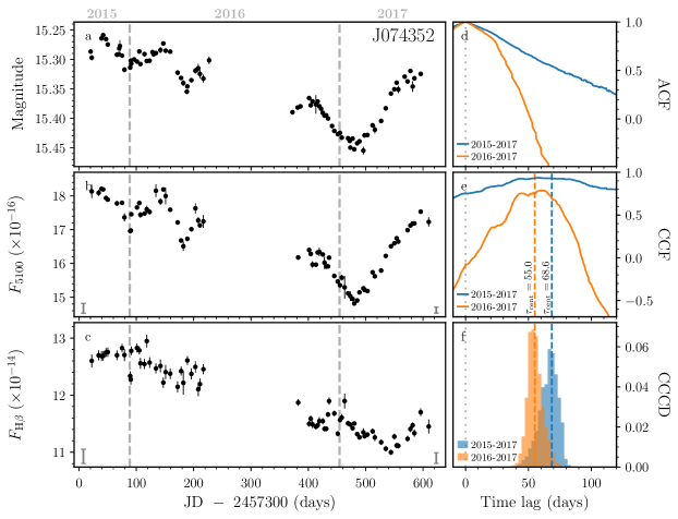
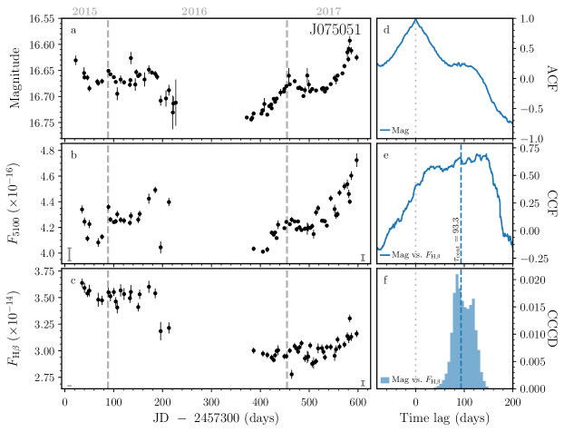
Figure 1: Light curves and cross-correlation functions. Panels a, b, c are the photometric, 5100 Å continuum, and H$\beta$ light curves. The name of the object is marked on the upper-right corner in panel a. The gray error bars in the lower-left and lower-right corners are the systematic errors in 2015 – 2016 and in 2016 – 2017, respectively (see more details in Section 3.1). The units of the continuum and emission-line light curves are ${\rm erg\ s^{-1}\ cm^{-2}\ \AA^{-1}}$ and ${\rm erg\ s^{-1}\ cm^{-2}}$, respectively. The gray dashed lines in panels a, b, c mark the beginnings (January 1st) of the different years. Panels d, e, f are the ACF, CCF, and the cross-correlation centroid distribution (CCCD) in the observed frame. The orange and blue colors in panels d, e, f indicate that we perform CCF analysis by using the entire light curves or the light curves in a single year. The gray dotted lines mark the zero time lags. The time lags in the observed frame are marked by the dashed lines (with the numbers beside) in panels e and f. For SDSS J075051, the time lag is obtained by the CCF of the photometric and H$\beta$ light curves. For SDSS J075949, we also plot its light curves in 2014–2015 from Paper V for comparison.

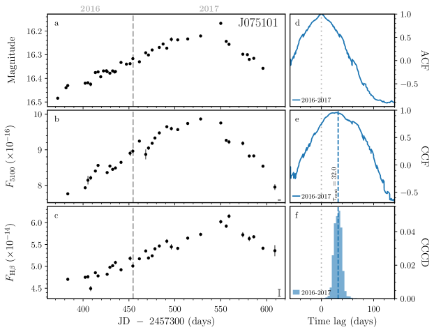
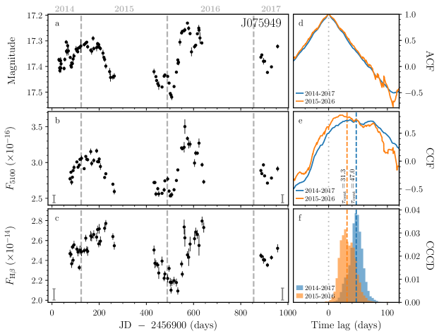
Figure 1: (Continued.)

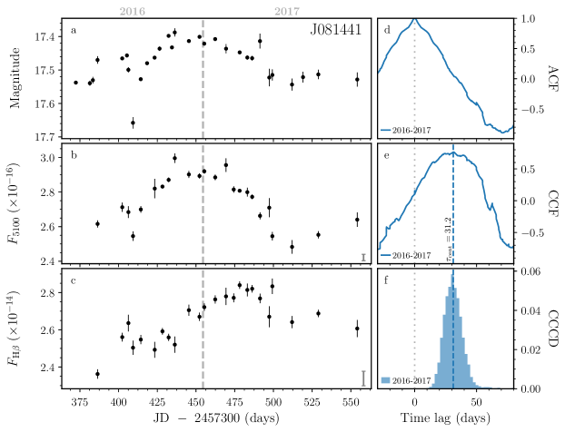
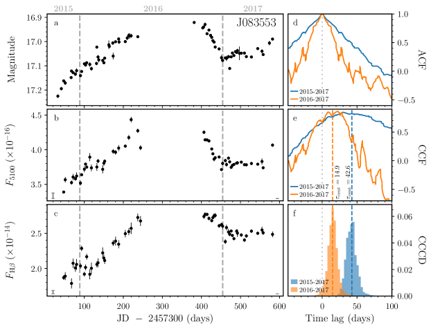
Figure 1: (Continued.)

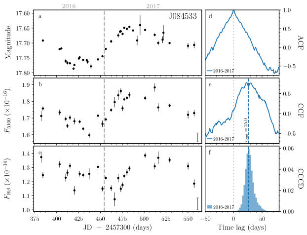
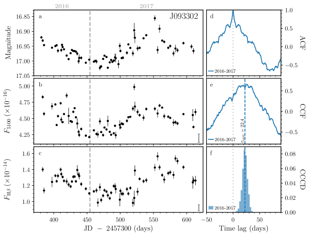
Figure 1: (Continued.)

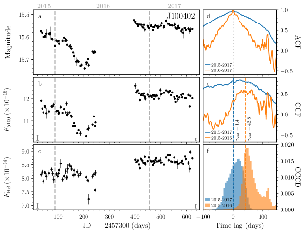
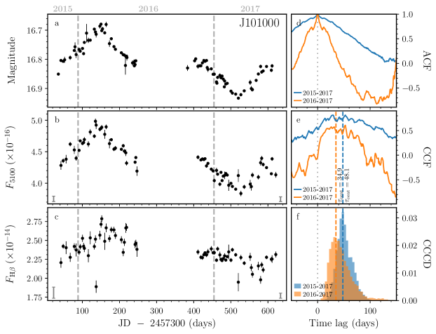
Figure 1: (Continued.)

3 Measurements of time lags, black hole masses, and accretion rates

3.1 Light Curves

After the data reduction and calibration, we can measure their continuum and H$\beta$ light curves from the calibrated spectra. The light curves can be obtained by two different approaches: (1) direct integration method and (2) spectral decomposition method. The first approach, widely used in most RM studies (e.g., Peterson et al. 1998; Kaspi et al. 2000; Bentz et al. 2009; Grier et al. 2012; Fausnaugh et al. 2017, Papers I, IV, and V), simply integrates the flux in the H$\beta$ band after subtracting the continuum determined by two nearby line-free windows. It applies to strong and isolated emission lines (e.g., H$\beta$) and works well both for the spectra with good or poor S/N. The second one measures the emission-line fluxes by multi-component spectral fitting, and has been gradually adopted in recent years (e.g., Barth et al. 2013, 2015, Paper III, and Lu et al. 2016). It can deblend and measure the fluxes of Fe ii or He ii lines, but has higher demand for the S/N of the spectra. The spectral decomposition approach can remove the contamination from Fe ii in the H$\beta$ flux measurements. However, given the better robustness of the integration method for spectra with moderate S/N, we adopt the direct integration approach, as a first step, to measure the continuum and H$\beta$ light curves in this paper. It should be noted that the two approaches do not give very different H$\beta$ lag measurements for the AGNs with high accretion rates (see Figure 6 in Paper III). We will measure their Fe ii light curves using the spectral decomposition method in a separate paper in the future.

We choose the continuum and the H$\beta$ windows that can avoid the contamination from the other emission lines (e.g., [O iii]$\lambda$4959, Fe ii, and He ii) as much as possible for each object (listed in Table 2). The continuum fluxes are set as the median values in the windows around 5100 Å in the rest frame. To measure the line light curves, we integrate the fluxes in the windows of H$\beta$ after subtracting the background beneath, which is determined by interpolating two nearby bands (blue and red continuum windows, see also in Figure 12 in Appendix C). The uncertainties in the light curves consist of two components: statistical noises originated from the Poisson process of photons and systematic uncertainties caused by poor weather conditions, bright moon, telescope tracking inaccuracies, slit positioning, etc. The Poisson noises are demonstrated as the error bars of the points in the light curves (see Figure 1). The systematic uncertainties are estimated by the median filter method (see more details in Paper I), and are marked as gray error bars in the lower-left corners (for the light curves taken in 2015 Oct – 2016 Jun) and lower-right corners (for the light curves taken in 2016 Oct – 2017 Jun) of panels b and c in Figure 1. Both the two components of the uncertainties are taken into account in the analysis of the following sections. The photometric light curves of the targets, the continuum light curves at 5100 Å  and H$\beta$ light curves are provided in Tables 3-7 and shown in Figure 1. We plot the photometric light curves to verify the calibration precision of the spectra. It is obvious that the calibration based on the comparison stars works fine, because the $r^{\prime}$-band light curves are consistent with the 5100 Å light curves (Figure 1). In addition, the photometric light curves can also be used as a substitute of the continuum, if the quality of the 5100 Å light curve is not good enough (see Section 3.3).

Table 3: Light curves of SDSS J074352 and SDSS J075051

SDSS J074352							SDSS J075051
Photometry			Spectra				Photometry			Spectra
JD	mag		JD	$F_{5100}$	$F_{\rm H\beta}$		JD	mag		JD	$F_{5100}$	$F_{\rm H\beta}$
20.379	$15.287\pm 0.002$		22.294	$18.134\pm 0.199$	$12.601\pm 0.111$		22.327	$16.631\pm 0.009$		35.306	$4.340\pm 0.031$	$3.638\pm 0.041$
22.273	$15.297\pm 0.004$		34.307	$18.091\pm 0.093$	$12.697\pm 0.089$		39.452	$16.655\pm 0.011$		40.308	$4.245\pm 0.032$	$3.591\pm 0.047$
39.335	$15.264\pm 0.002$		39.365	$18.210\pm 0.047$	$12.685\pm 0.084$		40.275	$16.663\pm 0.004$		46.294	$4.114\pm 0.022$	$3.539\pm 0.035$
42.259	$15.259\pm 0.002$		42.278	$18.192\pm 0.046$	$12.688\pm 0.085$		46.260	$16.664\pm 0.005$		50.345	$4.226\pm 0.031$	$3.565\pm 0.055$
47.215	$15.266\pm 0.002$		47.239	$17.938\pm 0.060$	$12.748\pm 0.077$		50.321	$16.684\pm 0.006$		68.430	$4.082\pm 0.034$	$3.480\pm 0.066$

Note. — JD: Julian dates from 2,457,300; $F_{5100}$ and $F_{{\rm H\beta}}$ are the continuum fluxes at 5100 Å and H$\beta$ fluxes in units of $10^{-16}\ {\rm erg\ s^{-1}\ cm^{-2}\ \AA^{-1}}$ and $10^{-14}\ {\rm erg\ s^{-1}\ cm^{-2}}$, respectively. This table is available in its entirety in a machine-readable form in the online journal. A portion is shown here for guidance regarding its form and content.

Table 4: Light curves of SDSS J075101 and SDSS J075949

SDSS J075101							SDSS J075949
Photometry			Spectra				Photometry			Spectra
JD	mag		JD	$F_{5100}$	$F_{\rm H\beta}$		JD	mag		JD	$F_{5100}$	$F_{\rm H\beta}$
372.376	$16.484\pm 0.003$		383.349	$7.762\pm 0.032$	$4.704\pm 0.037$		32.262	$17.420\pm 0.011$		32.298	$2.721\pm 0.022$	$2.505\pm 0.044$
381.415	$16.440\pm 0.003$		402.305	$7.932\pm 0.020$	$4.751\pm 0.027$		40.338	$17.440\pm 0.005$		36.308	$2.720\pm 0.023$	$2.371\pm 0.049$
383.314	$16.430\pm 0.004$		405.295	$8.144\pm 0.119$	$4.762\pm 0.042$		43.259	$17.455\pm 0.006$		40.372	$2.560\pm 0.032$	$2.368\pm 0.035$
402.274	$16.421\pm 0.002$		408.297	$8.210\pm 0.060$	$4.493\pm 0.058$		48.260	$17.467\pm 0.006$		48.295	$2.634\pm 0.024$	$2.354\pm 0.028$
405.267	$16.419\pm 0.004$		413.436	$8.402\pm 0.025$	$4.854\pm 0.031$		52.316	$17.474\pm 0.016$		52.343	$2.562\pm 0.043$	$2.274\pm 0.059$

Note. — JD: Julian dates from 2,457,300; $F_{5100}$ and $F_{{\rm H\beta}}$ are the continuum fluxes at 5100 Å and H$\beta$ fluxes in units of $10^{-16}\ {\rm erg\ s^{-1}\ cm^{-2}\ \AA^{-1}}$ and $10^{-14}\ {\rm erg\ s^{-1}\ cm^{-2}}$, respectively. This table is available in its entirety in a machine-readable form in the online journal. A portion is shown here for guidance regarding its form and content.

Table 5: Light curves of SDSS J081441 and SDSS J083553

SDSS J081441							SDSS J083553
Photometry			Spectra				Photometry			Spectra
JD	mag		JD	$F_{5100}$	$F_{\rm H\beta}$		JD	mag		JD	$F_{5100}$	$F_{\rm H\beta}$
372.380	$17.538\pm 0.005$		386.419	$2.616\pm 0.021$	$2.362\pm 0.025$		32.409	$17.225\pm 0.007$		47.340	$3.389\pm 0.016$	$1.870\pm 0.033$
381.419	$17.540\pm 0.008$		402.361	$2.712\pm 0.027$	$2.561\pm 0.024$		41.318	$17.194\pm 0.007$		51.329	$3.567\pm 0.039$	$1.890\pm 0.056$
383.377	$17.530\pm 0.010$		406.331	$2.684\pm 0.034$	$2.636\pm 0.045$		47.322	$17.162\pm 0.004$		67.384	$3.526\pm 0.030$	$1.787\pm 0.072$
386.391	$17.470\pm 0.011$		409.303	$2.545\pm 0.027$	$2.504\pm 0.038$		51.300	$17.171\pm 0.008$		71.340	$3.606\pm 0.045$	$2.074\pm 0.066$
402.333	$17.465\pm 0.003$		414.337	$2.699\pm 0.019$	$2.548\pm 0.025$		66.444	$17.148\pm 0.006$		77.278	$3.581\pm 0.026$	$2.008\pm 0.055$

Note. — JD: Julian dates from 2,457,300; $F_{5100}$ and $F_{{\rm H\beta}}$ are the continuum fluxes at 5100 Å and H$\beta$ fluxes in units of $10^{-16}\ {\rm erg\ s^{-1}\ cm^{-2}\ \AA^{-1}}$ and $10^{-14}\ {\rm erg\ s^{-1}\ cm^{-2}}$, respectively. This table is available in its entirety in a machine-readable form in the online journal. A portion is shown here for guidance regarding its form and content.

Table 6: Light curves of SDSS J084533 and SDSS J093302

SDSS J084533							SDSS J093302
Photometry			Spectra				Photometry			Spectra
JD	mag		JD	$F_{5100}$	$F_{\rm H\beta}$		JD	mag		JD	$F_{5100}$	$F_{\rm H\beta}$
384.333	$17.692\pm 0.004$		382.430	$1.712\pm 0.030$	$1.374\pm 0.038$		381.425	$16.920\pm 0.004$		383.413	$4.830\pm 0.026$	$1.401\pm 0.031$
403.406	$17.721\pm 0.003$		384.365	$1.757\pm 0.012$	$1.246\pm 0.021$		383.384	$16.931\pm 0.005$		385.389	$4.572\pm 0.029$	$1.138\pm 0.037$
405.430	$17.718\pm 0.003$		403.438	$1.734\pm 0.016$	$1.323\pm 0.023$		385.377	$16.947\pm 0.004$		397.442	$4.688\pm 0.051$	$1.245\pm 0.065$
410.298	$17.761\pm 0.006$		410.329	$1.695\pm 0.014$	$1.228\pm 0.027$		397.413	$16.955\pm 0.003$		402.425	$4.716\pm 0.019$	$1.324\pm 0.020$
412.309	$17.767\pm 0.005$		412.348	$1.653\pm 0.012$	$1.263\pm 0.022$		402.403	$16.950\pm 0.004$		404.389	$4.399\pm 0.017$	$1.254\pm 0.021$

Note. — JD: Julian dates from 2,457,300; $F_{5100}$ and $F_{{\rm H\beta}}$ are the continuum fluxes at 5100 Å and H$\beta$ fluxes in units of $10^{-16}\ {\rm erg\ s^{-1}\ cm^{-2}\ \AA^{-1}}$ and $10^{-14}\ {\rm erg\ s^{-1}\ cm^{-2}}$, respectively. This table is available in its entirety in a machine-readable form in the online journal. A portion is shown here for guidance regarding its form and content.

Table 7: Light curves of SDSS J100402 and SDSS J101000

SDSS J100402							SDSS J101000
Photometry			Spectra				Photometry			Spectra
JD	mag		JD	$F_{5100}$	$F_{\rm H\beta}$		JD	mag		JD	$F_{5100}$	$F_{\rm H\beta}$
33.422	$15.574\pm 0.005$		34.421	$11.915\pm 0.030$	$8.139\pm 0.074$		35.416	$16.851\pm 0.004$		42.430	$4.283\pm 0.069$	$2.206\pm 0.067$
34.398	$15.576\pm 0.005$		39.411	$11.558\pm 0.050$	$8.230\pm 0.084$		42.414	$16.804\pm 0.005$		48.400	$4.357\pm 0.035$	$2.422\pm 0.031$
39.383	$15.583\pm 0.004$		43.351	$11.387\pm 0.073$	$7.893\pm 0.093$		48.369	$16.807\pm 0.003$		56.349	$4.381\pm 0.068$	$2.403\pm 0.084$
43.330	$15.600\pm 0.005$		49.392	$11.684\pm 0.041$	$8.223\pm 0.054$		52.374	$16.802\pm 0.010$		67.324	$4.621\pm 0.034$	$2.276\pm 0.060$
49.365	$15.600\pm 0.003$		51.431	$11.630\pm 0.076$	$8.189\pm 0.066$		67.251	$16.794\pm 0.008$		78.342	$4.528\pm 0.064$	$2.420\pm 0.042$

Note. — JD: Julian dates from 2,457,300; $F_{5100}$ and $F_{{\rm H\beta}}$ are the continuum fluxes at 5100 Å and H$\beta$ fluxes in units of $10^{-16}\ {\rm erg\ s^{-1}\ cm^{-2}\ \AA^{-1}}$ and $10^{-14}\ {\rm erg\ s^{-1}\ cm^{-2}}$, respectively. This table is available in its entirety in a machine-readable form in the online journal. A portion is shown here for guidance regarding its form and content.

3.2 Cross-correlation Function

The interpolated cross-correlation function (ICCF; Gaskell & Sparke 1986; Gaskell & Peterson 1987) is adopted to determine the time delays of the H$\beta$ emission lines to the variation of the continuum light curves. We use the centroid of the part higher than a threshold (80% used here) in CCF as the measurement ($\tau_{\rm cent}$) of H$\beta$ time lag. The uncertainties of the lags are provided by the “flux randomization/random subset sampling (FR/RSS)” method, which takes into account both the errors of the points in the light curves and the uncertainties caused by the sampling/cadence for each individual object (see more details in Peterson et al., 1998, 2004). We adopt $\tau_{\rm cent}$ from the CCFs themselves instead of the median/mean values of the cross-correlation centroid distributions (CCCDs) produced by the FR/RSS method, to avoid any undiscovered bias to $\tau_{\rm cent}$ introduced by this method (occasionally, it overestimates the uncertainties, e.g., Peterson et al. 1998). The CCCDs are only used to estimate the error bars. But it should be noted that, in the present sample, the $\tau_{\rm cent}$ from the CCFs and the median/mean values of the CCCDs are highly consistent. Their differences are significantly smaller than the error bars (typically $\lesssim 10\%$ of the error bars), and can be ignored.

The auto-correlation functions (ACFs), CCFs and the distributions of the centroid time lags in the observed frame are shown in Figure 1. The time lags, their uncertainties, and the corresponding maximum correlation coefficients ($r_{\rm max}$) are listed in Table 8. For the objects monitored for more than one year, we also measured the H$\beta$ lags from the light curves only in 2015 Oct - 2016 Jun or in 2016 Oct - 2017 Jun. In some cases the $r_{\rm max}$ measured from the light curves in a single year is significantly higher than the values calculated from all the light curves, or uncertainties of the H$\beta$ lags are smaller because their ACFs are much narrower. We tend to use the time lags determined from the data in a single year, because the gaps in the light curves between the two years may introduce some uncertainties in the lag measurements. We discuss the light curves and the time delays for individual objects in the Section 3.3. The H$\beta$ time lags we used in the measurements of their BH masses are labeled by “$\surd$” in Table 8.

Table 8: Time Lags

			Observed		Rest-frame
Object	Period	$r_{\rm max}$	Time Lag		Time Lag	Note
			(days)		(days)
SDSS J074352	2015-2017	0.94	$68.6_{-10.2}^{+4.7}$		$54.8_{-8.1}^{+3.7}$
	2016-2017	0.79	$55.0_{-5.2}^{+6.6}$		$43.9_{-4.2}^{+5.2}$	$\surd$
SDSS J075051	2015-2017	0.69	$93.3_{-13.9}^{+26.2}$		$66.6_{-9.9}^{+18.7}$	$\surd$
SDSS J075101	2016-2017	0.96	$32.0_{-7.6}^{+6.3}$		$28.6_{-6.8}^{+5.6}$	$\surd$
SDSS J075949	2014-2017	0.74	$47.0_{-12.1}^{+10.3}$		$39.5_{-10.2}^{+8.7}$
	2015-2016	0.83	$31.3_{-11.3}^{+13.8}$		$26.4_{-9.5}^{+11.6}$	$\surd$
SDSS J081441	2016-2017	0.76	$31.2_{-6.9}^{+8.4}$		$26.8_{-5.9}^{+7.3}$	$\surd$
SDSS J083553	2015-2017	0.85	$42.6_{-7.6}^{+7.1}$		$35.4_{-6.3}^{+5.9}$
	2016-2017	0.86	$14.9_{-6.6}^{+6.5}$		$12.4_{-5.4}^{+5.4}$	$\surd$
SDSS J084533	2016-2017	0.78	$25.9_{-5.1}^{+9.5}$		$19.9_{-3.9}^{+7.3}$	$\surd$
SDSS J093302	2016-2017	0.66	$22.4_{-5.0}^{+4.5}$		$19.0_{-4.3}^{+3.8}$	$\surd$
SDSS J100402	2015-2017	0.84	$1.4_{-19.0}^{+31.6}$		$1.0_{-14.3}^{+23.8}$
	2016-2017	0.60	$42.8_{-5.5}^{+57.7}$		$32.2_{-4.2}^{+43.5}$	$\surd$
SDSS J101000	2015-2017	0.81	$48.1_{-10.5}^{+19.0}$		$38.2_{-8.4}^{+15.1}$
	2016-2017	0.61	$34.9_{-9.6}^{+29.5}$		$27.7_{-7.6}^{+23.5}$	$\surd$

Note. — “$\surd$” means we use this time lag of the object to calculate its BH mass. The lag of SDSS J075051 is obtained from its photometric and H$\beta$ light curves.

3.3 Notes on Individual Objects

SDSS J074352: Both the continuum and H$\beta$ light curves show very clear dips during 2016–2017. In general, the time lag measured from the light curves in 2016–2017 is consistent with the lag measured from its entire light curves, within the uncertainties. However, the ACF generated solely from its continuum light curve in 2016–2017 is much narrower than the ACF obtained from its entire continuum light curve. Considering that the season gap between 2016 Jun to 2016 Oct may influence the H$\beta$ lag measurement, we adopt the CCF analysis of the light curves in 2016–2017 as the final result of this object.

SDSS J075051: The quality of its photometric light curve is superior to the 5100 Å continuum light curve. The $r_{\rm max}$ of photometry vs. H$\beta$ is higher than the value ($\sim 0.4$) of 5100 Å vs. H$\beta$. More observations are needed to improve its lag measurement in the future.

SDSS J075101: It was monitored previously in 2013 Nov – 2014 May (Paper IV), yielding an H$\beta$ time lag of $33.4_{-5.6}^{+15.6}$ days in the rest frame. The new measurement in the present paper is consistent with the previous observations, within the uncertainties, but the error bars are smaller. The peak around Julian date 550 (from the zero point of 2457300 in Figure 1, similarly hereinafter) is prominent, and its $r_{\rm max}$ is very high (0.96).

SDSS J075949: We have monitored it for three years, from 2014 to 2017. The result of the first year was published in Paper V, showing relatively large error bars in its H$\beta$ time delay ($55.0_{-13.1}^{+17.0}$ days in the rest frame). We also plot its old light curves in 2014–2015 in Figure 1 for comparison. The new observation in this paper gives better constraints on the H$\beta$ lag. The light curves in 2015–2016 give a higher correlation coefficient ($r_{\rm max}=0.83$) than the value ($r_{\rm max}=0.74$) obtained from its entire light curves (including the data in 2014–2015). We thus use the CCF results from 2015–2016 in the analysis of the $R_{\rm H\beta}$–$L_{5100}$ relation. The new time lag is $26.4_{-9.5}^{+11.6}$ days in the rest frame. This is somewhat shorter than the previous value (Paper V), but considering the uncertainties, the difference is not significant.

SDSS J081441: Its light curves from 2013 Nov – 2014 May were published in Paper IV. In the H$\beta$ 2013 – 2014 light curve, there are only several points after the peak around Julian day 160 (see Figure 1 of Paper IV), because the altitude of the source was already too low to observe at the end. The new 2016 – 2017 light curves look more convincing, and the lag measurement is much better (with smaller error bars).

SDSS J083553: It is a little unfortunate that the primary peaks around Julian day $\sim$300 in the continuum and H$\beta$ light curves are invisible. However, the small dip close to Julian day $\sim$450 is observed clearly. So, we adopt the CCF analysis from the 2016–2017 data to be the final result for this object. Its ACF is narrower and the $r_{\rm max}$ is a little higher than the analysis obtained from the entire light curves from 2015 to 2017.

SDSS J084533: The time lag in the present paper is consistent with the previous value from 2014 – 2015 (Paper V). Its light curves from 2016 to 2017 show two large structures, a dip around Julian day 430 and a peak around Julian day 480, yielding a very robust lag measurement.

SDSS J093302: The big dip and its response are very clear in the light curves. The lag measurement is pretty reliable.

SDSS J100402: The centroid of the peak of the CCF calculated from the entire light curves is nearly zero because of the the gap between the two years and the very flat light curves in 2016 – 2017. Therefore, we adopt the light curves in 2015 – 2016 to measure the time lag. The uncertainty of its H$\beta$ lag is the largest among all of the objects in this paper.

SDSS J101000: The scatter and the error bars of the H$\beta$ light curve in 2016 – 2017 are smaller than those in 2015 – 2016. Thus, we select the lag measurement using the light curves in 2016 – 2017 as the final result. In general, the lags obtained from the light curves in 2015 – 2017 and in 2016 – 2017 are consistent with each other.

Table 9: H$\beta$ Width Measurements

	Mean Spectra			RMS Spectra
Object	FWHM	$\sigma_{{\rm H\beta}}$		FWHM	$\sigma_{{\rm H\beta}}$
	(km s-1)	(km s-1)		(km s-1)	(km s-1)
SDSS J074352	$3156\pm 36$	$1976\pm 10$		$3149\pm 92$	$1489\pm 32$
SDSS J075051	$1904\pm 9$	$1239\pm 5$		$970\pm 345$	$547\pm 46$
SDSS J075101	$1679\pm 35$	$1179\pm 14$		$1605\pm 630$	$987\pm 74$
SDSS J075949	$1783\pm 17$	$1135\pm 3$		$1661\pm 402$	$845\pm 40$
SDSS J081441	$1782\pm 16$	$1367\pm 6$		$1247\pm 1048$	$1195\pm 379$
SDSS J083553	$1758\pm 16$	$1015\pm 9$		$1642\pm 479$	$1234\pm 15$
SDSS J084533	$1297\pm 12$	$965\pm 7$		$1626\pm 98$	$1126\pm 9$
SDSS J093302	$1800\pm 25$	$1423\pm 7$		$1526\pm 313$	$838\pm 283$
SDSS J100402	$2088\pm 1$	$1425\pm 5$		$2555\pm 78$	$1173\pm 132$
SDSS J101000	$2311\pm 1$	$1409\pm 1$		$2237\pm 129$	$1386\pm 150$

3.4 Contribution of Host Galaxies

Generally, the contribution of host galaxies in the slit can be decomposed and removed from the 5100 Å luminosities of the objects by using the high-resolution image observations (e.g., from Hubble Space Telescope, HST). However, none of the objects, except SDSS J100402 (also known as PG 1001+291), has imaging observations from HST. As in Papers IV and V, we uniformly adopt the empirical relation proposed by Shen et al. (2011), to remove the host contribution in the 5100 Å luminosities. The luminosity ratio of host to AGN at 5100 Å can be expressed as $L_{5100}^{\rm host}/L_{5100}^{\rm AGN}=0.8052-1.5502x+0.912x^{2}-0.1577x^{3}$, for $x<1.053$, where $x=\log\left(L_{5100}^{\rm tot}/10^{44}{\rm erg~{}s^{-1}}\right)$ and $L_{5100}^{\rm tot}$ is the total luminosity at 5100 Å. For $x>1.053$, $L_{5100}^{\rm host}\ll L_{5100}^{\rm AGN}$, and the host contribution can be ignored. The fractions of host contamination in the total 5100 Å luminosities are 26.0%, 28.0%, 37.2%, 17.9%, 14.9%, 23.1%, and 6.8% for SDSS J075101, J075949, J081441, J083553, J084533, J093302, and J101000, respectively. The host contribution can be ignored for SDSS J074352, J075051, and J100402.

3.5 Black Hole Masses and Accretion Rates

We use Equation (1) to calculate the BH masses of the objects observed in SEAMBH2015–2016. The widths of the H$\beta$ emission lines can be obtained from the FWHM or $\sigma_{{\rm H\beta}}$ measured from their mean or RMS spectra. Different works adopt different line width measurements (e.g., Peterson et al. 2004; Bentz et al. 2009; Denney et al. 2010; Grier et al. 2012; Kaspi et al. 2005, Papers I-V). In general, the BH masses produced by the different line width measurements are consistent, because their corresponding virial factors $f_{\rm BLR}$ are calibrated, in the same way, by comparing the RM objects with measurements of bulge stellar velocity dispersion ($\sigma_{*}$) with the ${M_{\bullet}}-\sigma_{*}$ relation of inactive galaxies (e.g., Onken et al. 2004; Woo et al. 2010; Park et al. 2012; Grier et al. 2013; Ho & Kim 2014; Woo et al. 2015, see a brief review in Du et al. 2017). The exact value of $f_{\rm BLR}$ is still a matter of some debate and has large uncertainties. Recently, Woo et al. (2015) found that narrow-line Seyfert 1 (NLS1) galaxies (the H$\beta$ widths of most SEAMBHs conform to the definition of NLS1s) has a value of $f_{\rm BLR}$ = 1.12. On the other hand, Ho & Kim (2014) show that $f_{\rm BLR}$ is smaller than 1 for the AGNs with pseudobulges (NLS1s tend to host pseudobulges; e.g., Mathur et al. 2012). It is not clear will be the final value of $f_{\rm BLR}$. More observations are needed to calibrate $f_{\rm BLR}$ in the future. At this stage, as in the other papers in our series (Papers I-V), we adopt FWHM measured from the mean spectra and ${f_{\rm BLR}}=1$ to calculate the BH masses, but we acknowledge the large uncertainty on $f_{\rm BLR}$.

In order to measure the FWHM of broad H$\beta$, the narrow component of the line should be removed. This is done by fixing the flux of narrow H$\beta$ to 10% of the flux of [O iii] $\lambda 5007$ (the typical value in AGNs; e.g., Stern & Laor 2013; Kewley et al. 2006), and the uncertainty is estimated by setting H$\beta$$/$[O iii]$\lambda 5007$ to 0% and 20% as the lower and upper limit, respectively. Narrow H$\beta$ and [O iii] are weak in SEAMBHs; thus, the influence of the narrow-component subtraction to the measurements is not very significant. We measure FWHM of H$\beta$ from the mean spectra after removing the narrow component. For completeness, we also provide $\sigma_{{\rm H\beta}}$ measured from the mean spectra, and FWHM and $\sigma_{{\rm H\beta}}$ measured from the RMS spectra. The widths are measured from the RMS spectra after smoothing by a 9-pixel boxcar, and the uncertainties are obtained by comparing with the measurements from the profiles smoothed by a 3-pixel boxcar. The instrumental broadening (FWHM$\approx$1200 km s^-1), estimated from the spectra of the comparison stars, has been subtracted from the width measurements. The H$\beta$ line width and their uncertainties are listed in Table 9.

As in Papers IV and V, the dimensionless accretion rates of the objects are estimated by Equation (4) because we cannot observe their entire spectral energy distributions (SEDs). Equation (4) is derived from the thin accretion disk model (Shakura & Sunyaev 1973; Frank et al. 2002; see more details in Paper II), and can be used as a substitute for the traditional estimate of Eddington ratio (e.g., $L_{\rm bol}/L_{\rm Edd}=10L_{5100}/L_{\rm Edd}$, where $L_{\rm bol}$ is the bolometric luminosity and $L_{\rm Edd}$ is the Eddington Luminosity). Its validity has been discussed in the Appendix of Paper V, and it applies to ${\dot{\mathscr{M}}}\lesssim 3\times 10^{3}m_{7}^{-1/2}$, where $m_{7}={M_{\bullet}}/10^{7}M_{\odot}$. We list the BH masses, 5100 Å and H$\beta$ luminosities, and the accretion rates in Table 10.

As described in Papers II and V, the criterion of $\dot{\mathscr{M}}$ for identifying SEAMBHs still has some uncertainties (Laor & Netzer, 1989; Beloborodov, 1998; Sa̧dowski et al., 2011). We can use $\eta{\dot{\mathscr{M}}}\geq 0.1$ as the criterion, because the accretion disk becomes slim and the radiation efficiency gets reduced (Sa̧dowski et al., 2011), where $\eta$ is the mass-to-radiation conversion efficiency. To be conservative, we adopted the lowest $\eta$ (0.038, for retrograde disk with BH spin $a=-1$; see Bardeen et al. 1972). Thus, SEAMBHs are AGNs with ${\dot{\mathscr{M}}}\geq 2.63$. For simplicity, and as in other papers in this series, we use ${\dot{\mathscr{M}}}=3$ as the criterion to distinguish SEAMBHs from AGNs with low accretion rates.

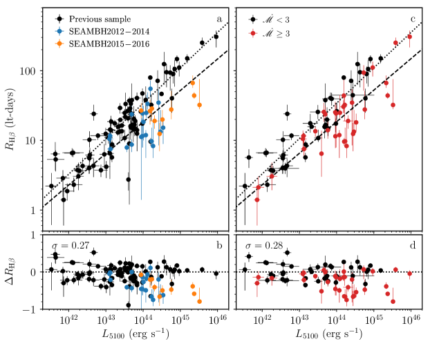
Figure 6: $R_{\rm H\beta}$–$L_{5100}$ relation. In panels a and b, each campaign for the objects with repeated RM observations is shown as a single point. In panels c and d, multiple observations for the same object have been averaged. The dotted and dashed lines are the linear regressions for the AGNs with ${\dot{\mathscr{M}}}<3$ and with ${\dot{\mathscr{M}}}\geq 3$, respectively. $\sigma$ is the standard deviation of the residual $\Delta{R_{\rm H\beta}}$. In the left panels, the blue and orange points are the SEAMBHs observed in our campaign, and the black points are the other RM objects. In the right panels, the red points are the objects with ${\dot{\mathscr{M}}}\geq 3$, and the black ones are the AGNs with low accretion rates.

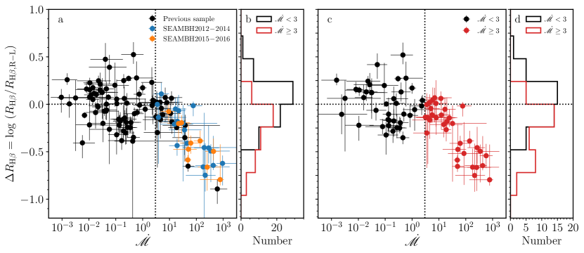
Figure 7: The correlation between $\Delta{R_{\rm H\beta}}$ and $\dot{\mathscr{M}}$. $\Delta{R_{\rm H\beta}}$ is the deviations of the SEAMBHs from the $R_{\rm H\beta}$–$L_{5100}$ relation of sub-Eddington sources. The meaning of the different colors in panels a and c are the same in Figure 6. Panels b and d show the distributions of $\Delta{R_{\rm H\beta}}$ in different subsamples in panels a and c. The vertical and horizontal dashed lines mark ${\dot{\mathscr{M}}}=3$ and $\Delta{R_{\rm H\beta}}=0$, respectively.

4 Properties of H$\beta$ lags in SEAMBHs

The time delays of the H$\beta$ emission lines in SEAMBHs have been shown to be shorter by a factor of 2 – 8 compared to AGNs with normal accretion rates, and the degree of shortening strongly correlates with the accretion rates (Papers IV and V). To investigate the magnitude of the shortening for the newly observed SEAMBHs with higher luminosities, we plot the $R_{\rm H\beta}$–$L_{5100}$ relation in Figure 6, including the SEAMBHs newly observed from 2015 to 2017, SEAMBHs published in Papers I – V, other objects compiled in Papers IV and V, and several newly observed AGNs studied by other groups published after Paper V. In the left panel of Figure 6, each campaign for the objects with repeated RM observations is treated as a single point (called “direct scheme”); in the right panel, multiple observations for the same object (called “averaged scheme” see more details in Paper IV) are averaged. It is obvious that the sample in the present paper, in general, is more luminous than that of our previous SEAMBH campaigns (except for the four objects previously observed in Papers IV and V). The objects in SEAMBH2015-2016 still show much shorter H$\beta$ lags than AGNs of the same luminosity with normal accretion rates.

4.1 The BLR Size-Luminosity Relation

Using the FITEXY algorithm as modified by Tremaine et al. (2002), we obtain the linear regression for the direct scheme

$$\log\frac{{R_{\rm H\beta}}}{{\rm ltd}}\!=\!\left\{\!\begin{array}[]{ll}\!(1.40\pm 0.03)\!+\!(0.43\pm 0.03)\log\ell_{44},&\!(\text{all}{\dot{\mathscr{M}}})\\ \!(1.53\pm 0.03)\!+\!(0.51\pm 0.03)\log\ell_{44},&\!({\dot{\mathscr{M}}}\!<\!3)\\ \!(1.26\pm 0.04)\!+\!(0.45\pm 0.05)\log\ell_{44},&\!({\dot{\mathscr{M}}}\!\geq\!3)\end{array}\right.$$ (5)

with intrinsic scatter $\sigma_{\rm in}=$ (0.21, 0.16, 0.22). For the averaged scheme, we find

$$\log\frac{{R_{\rm H\beta}}}{{\rm ltd}}\!=\!\left\{\!\begin{array}[]{ll}\!(1.39\pm 0.03)\!+\!(0.43\pm 0.03)\log\ell_{44},&\!(\text{all}{\dot{\mathscr{M}}})\\ \!(1.53\pm 0.04)\!+\!(0.51\pm 0.04)\log\ell_{44},&\!({\dot{\mathscr{M}}}\!<\!3)\\ \!(1.27\pm 0.05)\!+\!(0.45\pm 0.05)\log\ell_{44},&\!({\dot{\mathscr{M}}}\!\geq\!3)\end{array}\right.$$ (6)

with intrinsic scatter $\sigma_{\rm in}=$ (0.22, 0.17, 0.21). The intercepts of the correlations for the AGNs with high (${\dot{\mathscr{M}}}\geq 3$) and low (${\dot{\mathscr{M}}}<3$) accretion rates are significantly different. On average, the H$\beta$ lags of the ${\dot{\mathscr{M}}}\geq 3$ sources are shorter than the values of the ${\dot{\mathscr{M}}}<3$ sources by a factor of $\sim 2$ (0.26 dex). The slope of the SEAMBHs may be slightly smaller, although the difference is not very significant, considering the uncertainties. In view of the currently limited and its non-uniform distribution, especially at low and high luminosities, it is premature to draw firm conclusions on the slopes of the correlations. At this stage, as a preliminary result, the slopes of high- and low-${\dot{\mathscr{M}}}$ objects can be regarded as indistinguishable.

Table 10: Results of H$\beta$ Reverberation Mapping of the SEAMBHs in 2015 – 2017

Objects	$\tau_{{\rm H\beta}}$	FWHM	$\log{M_{\bullet}}$	$\log{\dot{\mathscr{M}}}$	$\log L_{5100}$	$\log L_{{\rm H\beta}}$	EW(H$\beta$)
	(days)	(km s-1)	($M_{\odot}$)		(erg s-1)	(erg s-1)	(Å)
SDSS J074352	$43.9_{-4.2}^{+5.2}$	$3156\pm 36$	$7.93_{-0.04}^{+0.05}$	$1.69_{-0.13}^{+0.12}$	$45.37\pm 0.02$	$43.48\pm 0.01$	$65.8\pm 3.5$
SDSS J075051	$66.6_{-9.9}^{+18.7}$	$1904\pm 9$	$7.67_{-0.07}^{+0.11}$	$2.14_{-0.24}^{+0.16}$	$45.33\pm 0.01$	$43.34\pm 0.03$	$51.9\pm 4.5$
SDSS J075101	$28.6_{-6.8}^{+5.6}$	$1679\pm 35$	$7.20_{-0.12}^{+0.08}$	$1.45_{-0.23}^{+0.30}$	$44.24\pm 0.04$	$42.38\pm 0.04$	$70.4\pm 9.0$
SDSS J075949	$26.4_{-9.5}^{+11.6}$	$1783\pm 17$	$7.21_{-0.19}^{+0.16}$	$1.34_{-0.42}^{+0.48}$	$44.19\pm 0.06$	$42.47\pm 0.04$	$98.9\pm 17.0$
SDSS J081441	$26.8_{-5.9}^{+7.3}$	$1782\pm 16$	$7.22_{-0.11}^{+0.10}$	$0.97_{-0.28}^{+0.28}$	$43.95\pm 0.04$	$42.39\pm 0.02$	$140.4\pm 16.2$
SDSS J083553	$12.4_{-5.4}^{+5.4}$	$1758\pm 16$	$6.87_{-0.25}^{+0.16}$	$2.41_{-0.35}^{+0.53}$	$44.44\pm 0.02$	$42.48\pm 0.02$	$56.1\pm 4.0$
SDSS J084533	$19.9_{-3.9}^{+7.3}$	$1297\pm 12$	$6.82_{-0.10}^{+0.14}$	$2.64_{-0.31}^{+0.22}$	$44.52\pm 0.02$	$42.60\pm 0.03$	$61.7\pm 5.1$
SDSS J093302	$19.0_{-4.3}^{+3.8}$	$1800\pm 25$	$7.08_{-0.11}^{+0.08}$	$1.79_{-0.40}^{+0.40}$	$44.31\pm 0.13$	$42.10\pm 0.05$	$31.8\pm 10.3$
SDSS J100402	$32.2_{-4.2}^{+43.5}$	$2088\pm 1$	$7.44_{-0.06}^{+0.37}$	$2.89_{-0.75}^{+0.13}$	$45.52\pm 0.01$	$43.54\pm 0.01$	$53.6\pm 1.3$
SDSS J101000	$27.7_{-7.6}^{+23.5}$	$2311\pm 1$	$7.46_{-0.14}^{+0.27}$	$1.70_{-0.56}^{+0.31}$	$44.76\pm 0.02$	$42.77\pm 0.02$	$52.6\pm 3.4$

Note. — $\tau_{{\rm H\beta}}$ (in the rest-frame) and FWHM are the same as in Tables 8 and 9; we list them here again for the convenience of inspection. $L_{5100}$ are the luminosities corresponding to the light curves used for $\tau_{{\rm H\beta}}$ measurements. The host contribution in $L_{5100}$ has been removed (see Section 3.4). Galactic extinction has been corrected using the maps of Schlafly & Finkbeiner (2011).

4.2 Dependence of BLR Size on Accretion Rate

According to Papers IV and V, the shortening of the H$\beta$ lags in SEAMBHs show a strong correlation with accretion rate. In order to test whether this correlation extends to SEAMBHs of even higher luminosities, we define, as in Papers IV and V, $\Delta{R_{\rm H\beta}}=\log({R_{\rm H\beta}}/R_{{\rm H\beta},R-L})$ to quantify the deviation from the $R_{\rm H\beta}$–$L_{5100}$ relation of the subsample with ${\dot{\mathscr{M}}}<3$ (i.e., $R_{{\rm H\beta},R-L}$ is the correlation for ${\dot{\mathscr{M}}}<3$ in Equations (5) or (6)). Figure 7 shows the correlation between $\Delta{R_{\rm H\beta}}$ and $\dot{\mathscr{M}}$, as well as the distributions of the AGNs with ${\dot{\mathscr{M}}}\geq 3$ and ${\dot{\mathscr{M}}}<3$ in the direct and averaged schemes. The objects with ${\dot{\mathscr{M}}}<3$ are located in both the two left quadrants of $\Delta{R_{\rm H\beta}}\geq 0$ and $\Delta{R_{\rm H\beta}}<0$. However, SEAMBHs (${\dot{\mathscr{M}}}\geq 3$) only appear in the quadrant with $\Delta{R_{\rm H\beta}}<0$, and their $\Delta{R_{\rm H\beta}}$ values significantly correlate with $\dot{\mathscr{M}}$ (Pearson’s correlation coefficient and null-probability are $-0.84$ and $4.8\times 10^{-13}$ for the direct scheme; the corresponding values are $-0.82$ and $1.4\times 10^{-9}$ for the average scheme). The objects in SEAMBH2015–2016 follow the same correlation as those SEAMBHs with lower luminosities observed in our campaign between 2012 and 2015. The dependence on accretion rate for SEAMBHs of the $R_{\rm H\beta}$ deviations from the $R_{\rm H\beta}$–$L_{5100}$ relation can be obtained by the regression for the objects with ${\dot{\mathscr{M}}}\geq 3$:

$$\Delta{R_{\rm H\beta}}\!=\!\left\{\!\begin{array}[]{ll}\!(0.36\pm 0.08)\!-\!(0.44\pm 0.05)\log{\dot{\mathscr{M}}},&\!\text{(direct)}\\ \!(0.30\pm 0.09)\!-\!(0.40\pm 0.06)\log{\dot{\mathscr{M}}},&\!\text{(averaged)}\end{array}\right.$$ (7)

with intrinsic scatter $\sigma_{\rm in}=(0.04,0.07)$.

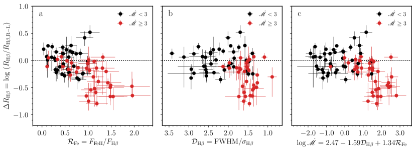
Figure 8: $\Delta{R_{\rm H\beta}}$ vs. ${\cal R}_{\rm Fe}$, ${\cal D}_{{\rm H\beta}}$, and $\dot{\mathscr{M}}$ derived from the fundamental plane. The repeated observations for the same objects have been averaged as in the right panels of Figures 6 and 7 (average scheme). For comparison, the axis of ${\cal D}_{{\rm H\beta}}$ is plotted inversely.

5 Discussion

5.1 Shortening of H$\beta$ Lags in SEAMBHs

Principal component analysis has reveal that the main variance of quasar optical spectra is a strong correlation between the flux ratio of broad Fe ii to H$\beta$ emission, the strength of [O iii]$\lambda 5007$, and the width of H$\beta$ (Boroson & Green, 1992; Sulentic et al., 2000a). The so-called Eigenvector 1 has been demonstrated to be driven by Eddington ratio $L_{\rm bol}/L_{\rm Edd}$ (Boroson & Green, 1992; Sulentic et al., 2000a, b; Marziani et al., 2003; Shen & Ho, 2014). AGNs with high Eddington ratios/accretion rates, such as NLS1s, show very strong Fe ii emission compared with normal sources (Boroson & Green, 1992; Hu et al., 2008a; Dong et al., 2011). And at the same time, the H$\beta$ profiles of NLS1s tend to be more Lorentzian (smaller values of ${\cal D}_{{\rm H\beta}}$) than those of broader line AGNs, which probably have more normal accretion rates (Véron-Cetty et al., 2001; Zamfir et al., 2010; Kollatschny & Zetzl, 2011).

Du et al. (2016c) recently investigated the correlation between the strength of Fe ii, the H$\beta$ profile, and the accretion rates of the RM AGN sample. They found that both the relative strength of optical Fe ii lines (${{\cal R}_{\rm Fe}}=F_{\rm Fe}/F_{{\rm H\beta}}$) and the H$\beta$ profile shape parameter (${\cal D}_{{\rm H\beta}}$ = FWHM/$\sigma_{{\rm H\beta}}$) indeed correlate with accretion rate $\dot{\mathscr{M}}$, where $F_{\rm Fe}$ is the flux of Fe ii in the region 4434–4684 Å and $F_{{\rm H\beta}}$ is the flux of broad H$\beta$. Combining ${\cal D}_{{\rm H\beta}}$ and ${\cal R}_{\rm Fe}$, they proposed a bivariate correlation of the form $\log{\dot{\mathscr{M}}}=\alpha_{2}+\beta_{2}{{\cal D}_{{\rm H\beta}}}+\gamma_{2}{{\cal R}_{\rm Fe}}$, termed the “BLR fundamental plane.” Thus, we can use ${\cal R}_{\rm Fe}$ and ${\cal D}_{{\rm H\beta}}$ as proxies of accretion rate to test the dependence of $\Delta{R_{\rm H\beta}}$ on accretion rate.

Figure 8 shows the correlation between $\Delta{R_{\rm H\beta}}$ and ${\cal R}_{\rm Fe}$, ${\cal D}_{{\rm H\beta}}$, or the $\dot{\mathscr{M}}$ derived from the fundamental plane. For comparison, the axis of ${\cal D}_{{\rm H\beta}}$ is plotted inversely. In general, the objects with larger ${\cal R}_{\rm Fe}$ and smaller ${\cal D}_{{\rm H\beta}}$ deviate more extremely from the $R_{\rm H\beta}$–$L_{5100}$ relation. ${\cal R}_{\rm Fe}$ and ${\cal D}_{{\rm H\beta}}$ are purely observables; thus, using them as proxies of $\dot{\mathscr{M}}$ can avoid the implicit enhancement to the $\Delta{R_{\rm H\beta}}$–$\dot{\mathscr{M}}$ correlation caused by the fact that $\dot{\mathscr{M}}$ is a derived quantity. The scatter of the $\dot{\mathscr{M}}$–${\cal R}_{\rm Fe}$ and $\dot{\mathscr{M}}$–${\cal D}_{{\rm H\beta}}$ correlations is relatively large (see Figure 1 in Du et al. 2016c). So, the $\Delta{R_{\rm H\beta}}$–${\cal R}_{\rm Fe}$ and $\Delta{R_{\rm H\beta}}$–${\cal D}_{{\rm H\beta}}$ correlations in panels a and b of Figure 8 are not as good as the $\Delta{R_{\rm H\beta}}$–$\dot{\mathscr{M}}$ correlation in Figure 7. Panel c in Figure 8 shows $\Delta{R_{\rm H\beta}}$ versus $\dot{\mathscr{M}}$ derived from the fundamental plane, which has smaller scatter than each of the single correlations ($\dot{\mathscr{M}}$–${\cal R}_{\rm Fe}$ or $\dot{\mathscr{M}}$–${\cal D}_{{\rm H\beta}}$). In consideration of the relatively large scatter in the $\dot{\mathscr{M}}$–${\cal R}_{\rm Fe}$ and $\dot{\mathscr{M}}$–${\cal D}_{{\rm H\beta}}$ correlations, and the fundamental plane, we do not attempt to apply linear regression to Figure 8. They are just used to demonstrate the validity of Equation (7) in different ways.

5.2 Self-shadowing Effect of Slim Disks on Lags

It has been predicted that the self-shadowing effects of slim accretion disks leads to a shrinking of the ionization front of the BLR, so that the H$\beta$ lag shortens with increasing accretion rate (Wang et al., 2014c). Because of radiation pressure, the inner part of the slim disk is not geometrically thin, a property that naturally leads to anisotropic ionizing continuum. The vertical thickness of the inner slim disk significantly suppresses the amount of the ionizing photons that can be received by the BLR clouds, although it does not change the continuum flux obtained by observers. If the ionization parameter remains constant for the H$\beta$ line, the radius at which H$\beta$ emits most efficiently will shrink significantly (see more details in Wang et al. 2014c). This was first evidenced in the SEAMBH2013–2014 samples (Papers IV and V). The current SEAMBH2015–2016 sample continues to lend support to the idea that the shortened H$\beta$ lags arise from self-shadowing effects of a slim disk.

Self-shadowing effects also depend on BLR geometry. According to the opening angle of slim disk ($\Delta\Omega_{\rm disk}$), the BLR can be divided into two parts: 1) a shadowed region and 2) an unshadowed region (Wang et al., 2014c). If BLRs originate from inflows from the dusty torus to the central BH, as suggested by Wang et al. (2017), the BLR opening angle ($\Delta\Omega_{\rm BLR}$) should follow the torus ($\Delta\Omega_{\rm torus}$). Namely, $\Delta\Omega_{\rm BLR}\sim\Delta\Omega_{\rm torus}$. In the regime of the standard accretion disk, $\Delta\Omega_{\rm disk}>\Delta\Omega_{\rm BLR}$, and the entire BLR is illuminated by the radiation of the disk. In the case of a slim disk, for a simple consideration, the relative size of the shadowed and unshadowed regions depends on $\Delta\Omega_{\rm disk}$ and $\Delta\Omega_{\rm torus}$. The shadowed region receives less ionizing luminosity than the unshadowed region. This may give rise to shrinkage of the ionization front in the shadowed regions, thereby leading to shortened H$\beta$ lags in SEAMBHs. This is a key prediction of the self-shadowing effects in SEAMBHs. Although shortened lags have been observed by the SEAMBH project, the relatively longer ones of the unshadowed regions have not yet been reported. A possible reason is that our current continuous period of monitoring is still not long enough because of the regular rainy season from June to October in the Lijiang site.

We note that the measurement of the H$\beta$ lag may possibly be influenced by the characteristic continuum variability timescale (Goad & Korista, 2014). The extremely short variability timescale (much shorter than the intrinsic H$\beta$ lag or the centroid of the one-dimensional transfer function) may lead to shortening of the lag measurement (see more detals in Goad & Korista, 2014). However, the variation timescales of the objects in this paper are typically much larger than their H$\beta$ time delays (the timescales are typically $\sim$100–300 days). Thus, the variation timescale is unlikely the dominant factor for the shortening of the H$\beta$ lags.

5.3 Results from the SDSS-RM campaign

The large sample size of the Sloan Digital Sky Survey RM (SDSS-RM) project (Shen et al., 2015) offers a promising opportunity to probe BHs with a large range of accretion rates and spins. Grier et al. (2017) recently reported H$\beta$ time lags detected in the first year of SDSS-RM. They successfully measured H$\beta$ lags for 44 SDSS targets mainly using the Bayesian-based modeling code JAVELIN (Zu et al., 2011) and the Continuum REprocessing AGN MCMC software (CREAM; Starkey et al. 2016) instead of the traditional ICCF. Interestingly, they, too, found shortened H$\beta$ lags compared with the canonical $R_{\rm H\beta}$–$L_{5100}$ relation for a number of objects. We plot the 44 objects in the $\Delta{R_{\rm H\beta}}$–$\dot{\mathscr{M}}$ plane in Figure 9; the black and red points are the same objects in Figure 7. The time lags, luminosities, and BH masses are taken directly from Grier et al. (2017), and their accretion rates ${\dot{\mathscr{M}}}$ are calculated using Equation (4). There are two extreme cases (SDSS J142052.44+525622.4 and SDSS JJ141856.19+535845.0) that show $\Delta{R_{\rm H\beta}}\approx-1$ and ${\dot{\mathscr{M}}}\approx 10^{-0.4\sim-0.5}$. A couple of objects with ${\dot{\mathscr{M}}}\gtrsim 3$ are in the SEAMBH regime. These conform to our expectation that high $\dot{\mathscr{M}}$ leads to shortened H$\beta$ lags. Surprisingly, some low-$\dot{\mathscr{M}}$ objects also have H$\beta$ lags much shorter than the $R_{\rm H\beta}$–$L_{5100}$ relation. What is the physical explanation for these?

One possible interpretation is that this is a signature of retrograde accretion onto the BH in low-accretion rate AGNs. In the accretion rate regime of the Shakura-Sunyaev disk (${\dot{\mathscr{M}}}\lesssim 3$), the inner edge of the disk is fully determined by the last stable radius (Bardeen et al., 1972), since the dissipation of gravitational energy via viscosity can be neglected within this radius (Page & Thorne, 1974). Different from the Shakura-Sunyaev disk, the inner edge of a slim disk is mostly determined by the accretion rate instead of the spin because the dissipation cannot be neglected (Watarai & Mineshige, 2003). As a consequence, except for accretion rate, the ionizing luminosity highly depends on the spin and hence seriously influences the ionization front of the BLR (Wang et al., 2014b). In the Shakura–Sunyaev regime, the ionizing luminosity of H$\beta$ shows a non-monotonic correlation with the 5100 Å luminosity if the quasar is undergoing retrograde accretion (see Figure 3 in Wang et al. 2014b). A cold disk in retrograde accretion leads to the inefficient generation of the ionizing continuum, causing the H$\beta$ region to become smaller than the case of prograde accretion (Wang et al., 2014b). For the extreme case of retrograde accretion onto a maximally rotating BH, the H$\beta$ lags are expected to be shortened by a factor of $\sim 10$ (Wang et al., 2014b). The two extreme cases from the SDSS-RM campaign may be caused by retrograde accretion.

In Figure 9, we divide the regime of accretion rates by ${\dot{\mathscr{M}}}\approx 3$. H$\beta$ lags are influenced jointly by the spin and the accretion rate below ${\dot{\mathscr{M}}}\approx 3$, and purely by accretion rate for ${\dot{\mathscr{M}}}\gtrsim 3$. The first regime is spin-driven, the second ${\dot{\mathscr{M}}}$-driven. The canonical $R_{\rm H\beta}$–$L_{5100}$  relation only holds for AGNs in the Shakura-Sunyaev regime. Our proposal should be tested by larger samples covering the widest possible range of accretion rates.

The discovery of retrograde accretion onto BHs in AGNs through RM campaigns, if confirmed by independent measurements (e.g., iron K$\alpha$ observations from X-ray spectra), has important implications for the cosmological evolution of BHs. It has been suggested that the spin angular momentum of BHs originates from accretion if the mass of the BH gained through accretion is larger than one-third of its original mass (e.g., Thorne 1974). Therefore, the direction of ongoing accretion may be different from the current spins obtained from past accretion episodes. The cosmological evolution of the radiation efficiency of $z\lesssim 2$ quasars (Wang et al., 2009; Li et al., 2012) suggests that BHs spinning down with cosmic time. This is confirmed by simulations of BH evolution (Volonteri et al., 2013; Tucci & Volonteri, 2017). The SDSS-RM discovery of shortened lags for AGNs with low accretion rates supports spin-down evolution.

Additionally, the truncated accretion disk of a BH with low accretion rate is plausibly responsible for the shortened H$\beta$ lag. In such an accretion disk, the linear $L_{5100}-L_{13.6\rm eV}$ relation will be broken since the ionizing photons are suppressed due to inefficient radiation in the evaporated part of the advection-dominated accretion flow, where $L_{13.6\rm eV}$ is the ionizing luminosity at 13.6 eV. Details will be presented in a forthcoming paper (Czerny & Wang in preparation). Broadband spectral energy distributions are needed for these low-accretion AGNs with shortened lags in order to distinguish the two possible mechanisms.

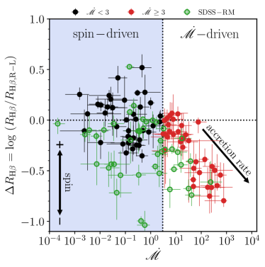
Figure 9: The $\Delta{R_{\rm H\beta}}-{\dot{\mathscr{M}}}$ plane, including the SDSS-RM sample. The plane is roughly divided into two regimes, at ${\dot{\mathscr{M}}}\approx 3$. Low-$\dot{\mathscr{M}}$ AGNs have a large scatter in $\Delta{R_{\rm H\beta}}$, whereas $\Delta{R_{\rm H\beta}}$ is inversely correlated with $\dot{\mathscr{M}}$ in the high-$\dot{\mathscr{M}}$ regime. The shortening of H$\beta$ lags in low-$\dot{\mathscr{M}}$ AGNs could be explained by retrograde accretion onto BHs. The arrows mark the physical drivers for the shortening of H$\beta$ lags in different accretion regimes.

6 Summary

We present the observational results of our reverberation mapping campaign of super-Eddington accreting massive black holes (SEAMBHs) completed during 2015 – 2017. We successfully measured H$\beta$ time lags for 10 SEAMBHs. Six out of the 10 objects have, on average, higher 5100 Å luminosities than the previous SEAMBHs. The other four targets are found to have H$\beta$ lags, in general, consistent with those previously measured during 2013 – 2015. The new observations significantly enlarge the size of the SEAMBH RM sample and improve the completeness of the SEAMBH sample at the high-luminosity end of the $R_{\rm H\beta}$–$L_{5100}$ relation. The SEAMBH samples show that their H$\beta$ time lags deviate from the $R_{\rm H\beta}$–$L_{5100}$ relation by a factor of 2 – 6 at fixed luminosity. The H$\beta$ lags decreases from the canonical $R_{\rm H\beta}$–$L_{5100}$ relation with increasing Fe ii/H$\beta$ flux ratio and change of H$\beta$ profile. The recent discovery by the SDSS-RM collaboration of H$\beta$ lags in AGNs with low accretion rates may signify retrograde accretion onto BHs. This has important implications for BH spins.

Appendix A Light Curves of Comparison Stars

In order to ensure that the comparison stars do not vary significantly during the campaign, we examine their light curves by performing differential photometry. Several other stars in the same field were used. The light curves of the comparison stars and their standard deviations are shown in Figure 10. None of the comparison stars shows strong variations during our observation period. The typical standard deviation is smaller than $\sim 2\%$.

Figure 10: The photometric light curves of the comparison stars in the slit.

Appendix B Evaluation to Calibration Precision

To show the precision of the comparison-star calibration, we plot the [O iii] light curve of SDSS J075101 after the calibration. This object is the one that has the strongest [O iii] in the sample; it has relatively weak Fe ii and high S/N. Its [O iii] fluxes are measured by a simple multi-component fitting (similar to Paper III): we model the broad H$\beta$ line with two Gaussians, each of the other lines ([O iii] $\lambda\lambda 4959,5007$, narrow H$\beta$, and He ii) with one Gaussian, the Fe ii using the template from Boroson & Green (1992), and the continuum with a power law. The scatter of its [O iii] flux is 3.0% (Figure 11), which can be regarded as an estimate of the calibration precision. However, it should be noted that the fitting itself may introduce large uncertainty to the [O iii] flux measurement, because [O iii] is too weak and Fe ii is relatively strong in SEAMBHs. Thus, the value of 3.0% is only an upper limit on the calibration uncertainty. For the other objects with weaker [O iii], stronger Fe ii, and lower S/N, it is difficult to obtain reliable [O iii] light curves.

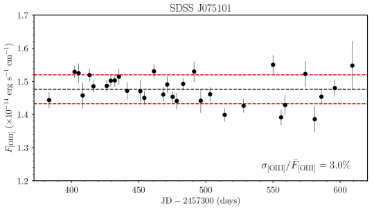
Figure 11: [O iii] light curve of SDSS J075101. The black dashed line marks the average value of [O iii] fluxes, and the red dashed lines mark the $\pm 1\sigma$ standard deviation. The ratio between the standard deviation and the mean value is 3.0%.

Appendix C Mean and RMS spectra

To illustrate the general spectral characteristics of each object, we plot their mean spectra and root-mean-square (RMS) spectra in Figure 12. Following the procedures in Papers IV and V, the mean and RMS spectra are defined, respectively, as

$$\bar{F}_{\lambda}=\frac{1}{N}\sum_{i=1}^{N}F_{\lambda}^{i},$$ (C1)

and

$$S_{\lambda}=\left[\frac{1}{N}\sum_{i=1}^{N}\left(F_{\lambda}^{i}-\bar{F}_{\lambda}\right)^{2}\right]^{1/2}.$$ (C2)

$F_{\lambda}^{i}$ is the $i$-th spectrum of the object, and $N$ is the number of spectra it has. It is obvious that their Fe ii emission lines are strong and [O iii] lines are extremely weak, which are the typical characteristics of AGNs with high accretion rates (see, e.g., Boroson & Green, 1992; Shen & Ho, 2014).

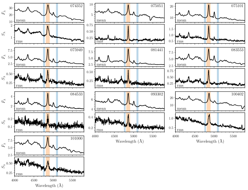
Figure 12: Mean and RMS spectra (observed flux vs. rest-frame wavelength) of the objects. The orange and blue regions are the windows for H$\beta$ emission lines and their backgrounds. The unit is ${10^{-16}\ \rm erg\ s^{-1}\ cm^{-2}\ \AA^{-1}}$.

References

- Bahcall et al. (1972) Bahcall, J. N., Kozlovsky, B.-Z., & Salpeter, E. E. 1972, ApJ, 171, 467
- Bardeen et al. (1972) Bardeen, J. M., Press, W. H., Teukolsky, S. A. 1972, ApJ, 178, 347
- Barth et al. (2015) Barth, A. J., Bennert, V. N., Canalizo, G., et al. 2015, ApJS, 217, 26
- Barth et al. (2013) Barth, A. J., Pancoast, A., Bennert, V. N., et al. 2013, ApJ, 769, 128
- Barth et al. (2011) Barth. A. J., Pancoast, A., Thorman, S. J., et al. 2011, ApJ, 743, 4
- Beloborodov (1998) Beloborodov, A. M. 1998, MNRAS, 297, 739
- Bentz et al. (2016) Bentz, M. C., Batiste, M., Seals, J., et al. 2016, ApJ, 831, 2
- Bentz et al. (2016) Bentz, M. C., Cackett, E. M., Crenshaw, D. M., et al. 2016, ApJ, 830, 136
- Bentz et al. (2013) Bentz, M. C., Denney, K. D., Grier, C. J., et al. 2013, ApJ, 767, 149
- Bentz et al. (2008) Bentz, M. C., Walsh, J. L., Barth, A. J., et al. 2008, ApJ, 689, L21
- Bentz et al. (2009) Bentz, M. C., Walsh, J. L., Barth, A. J., et al. 2009, ApJ, 705, 199
- Blandford & McKee (1982) Blandford, R. D., & McKee, C. F. 1982, ApJ, 255, 419
- Boroson & Green (1992) Boroson, T. A., & Green, R. F. 1992, ApJS, 80, 109
- Denney et al. (2009) Denney, K. D., Peterson, B. M., Pogge, R. W., et al. 2009, ApJ, 704, L80
- Denney et al. (2010) Denney, K. D., Peterson, B. M., Pogge, R. W., et al. 2010, ApJ, 721, 715
- Dong et al. (2011) Dong, X.-B., Wang, J.-G., Ho, L. C., et al. 2011, ApJ, 736, 86
- Du et al. (2014) Du, P., Hu, C., Lu, K.-X., et al. (SEAMBH Collaboration) 2014, ApJ, 782, 45 (Paper I)
- Du et al. (2015) Du, P., Hu, C., Lu, K.-X., et al. (SEAMBH Collaboration) 2015, ApJ, 806, 22 (Paper IV)
- Du et al. (2016a) Du, P., Lu, K.-X., Hu, C., et al. (SEAMBH Collaboration) 2016a, ApJ, 820, 27 (Paper VI)
- Du et al. (2016b) Du, P., Lu, K.-X., Zhang, Z.-X., et al. (SEAMBH Collaboration) 2016b, ApJ, 825, 126 (Paper V)
- Du et al. (2016c) Du, P., Wang, J.-M., Hu, C., et al. 2016c, ApJ, 818, L14
- Du et al. (2017) Du, P., Wang, J.-M., & Zhang, Z.-X. 2017, ApJ, 840, L6
- Fausnaugh (2017) Fausnaugh, M. M. 2017, PASP, 129, 024007
- Fausnaugh et al. (2017) Fausnaugh, M. M., Grier, C. J., Bentz, M. C., et al. 2017, ApJ, 840, 97
- Fischer et al. (2014) Fischer, T. C., Crenshaw, D. M., Kraemer, S. B., Schmitt, H. R., & Turner, T. J. 2014, ApJ, 785, 25
- Frank et al. (2002) Frank, J., King, A., & Raine, D. J. 2002, Accretion Power in Astrophysics, by Juhan Frank and Andrew King and Derek Raine, pp. 398. ISBN 0521620538. Cambridge, UK: Cambridge University Press, February 2002., 398
- Gaskell & Peterson (1987) Gaskell, C. M., & Peterson, B. M. 1987, ApJS, 65, 1
- Gaskell & Sparke (1986) Gaskell, C. M., & Sparke, L. S. 1986, ApJ, 305, 175
- Goad & Korista (2014) Goad, M. R., & Korista, K. T. 2014, MNRAS, 444, 43
- Grier et al. (2013) Grier, C. J., Martini, P., Watson, L. C., et al. 2013, ApJ, 773, 90
- Grier et al. (2012) Grier, C. J., Peterson, B. M., Pogge, R. W., et al. 2012, ApJ, 755, 60
- Grier et al. (2017) Grier, C. J., Trump, J. R., Shen, Y., et al. 2017, arXiv:1711.03114
- Ho & Kim (2014) Ho, L. C., & Kim, M. 2014, ApJ, 789, 17
- Ho & Kim (2015) Ho, L. C., & Kim, M. 2015, ApJ, 809, 123
- Horne (1994) Horne, K. 1994, Reverberation Mapping of the Broad-Line Region in Active Galactic Nuclei, 69, 23
- Hu et al. (2015) Hu, C., Du, P., Lu, K.-X., et al. (SEAMBH Collaboration) 2015, ApJ, 804, 138 (Paper III)
- Hu et al. (2008a) Hu, C., Wang, J.-M., Ho, L. C., et al. 2008a, ApJ, 687, 78-96
- Hu et al. (2008b) Hu, C., Wang, J.-M., Ho, L. C., et al. 2008b, ApJ, 683, L115
- Hu et al. (2016) Hu, C., Wang, J.-M., Ho, L. C., et al. 2016, ApJ, 832, 197
- Jiang et al. (2016) Jiang, L., Shen, Y., McGreer, I. D., et al. 2016, ApJ, 818, 137
- Kaspi et al. (2007) Kaspi, S., Brandt, W. N., Maoz, D., et al. 2007, ApJ, 659, 997
- Kaspi et al. (2005) Kaspi, S., Maoz, D., Netzer, H., et al. 2005, ApJ, 629, 61
- Kaspi et al. (2000) Kaspi, S., Smith, P. S., Netzer, H., et al. 2000, ApJ, 533, 631
- Kollatschny & Zetzl (2011) Kollatschny, W., & Zetzl, M. 2011, Nature, 470, 366
- Koshida et al. (2014) Koshida, S., Minezaki, T., Yoshii, Y., et al. 2014, ApJ, 788, 159
- Kewley et al. (2006) Kewley, L. J., Groves, B., Kauffmann, G., & Heckman, T. 2006, MNRAS, 372, 961
- Laor & Netzer (1989) Laor, A., & Netzer, H. 1989, MNRAS, 238, 897
- Li et al. (2012) Li, Y.-R., Wang, J.-M., & Ho, L. C. 2012, ApJ, 749, 187
- Li et al. (2018) Li, Y.-R., Songsheng, Y.-Y., Qiu, J., et al. (SEAMBH Collaboration) 2018, ApJ, submitted (Paper VIII)
- Lu et al. (2016) Lu, K.-X., Du, P., Hu, C., et al. 2016, ApJ, 827, 118
- Marziani et al. (2003) Marziani, P., Zamanov, R. K., Sulentic, J. W., & Calvani, M. 2003, MNRAS, 345, 1133
- Mathur et al. (2012) Mathur, S., Fields, D., Peterson, B. M., & Grupe, D. 2012, ApJ, 754, 146
- McLure & Dunlop (2002) McLure, R. J., & Dunlop, J. S. 2002, MNRAS, 331, 795
- Onken et al. (2004) Onken, C. A., Ferrarese, L., Merritt, D., et al. 2004, ApJ, 615, 645
- Page & Thorne (1974) Page, D. N. & Thorne, K. S. 1974, ApJ, 191, 499
- Pancoast et al. (2014) Pancoast, A., Brewer, B. J., Treu, T., et al. 2014, MNRAS, 445, 3073
- Park et al. (2012) Park, D., Kelly, B. C., Woo, J.-H., & Treu, T. 2012, ApJS, 203, 6
- Peterson et al. (1993) Peterson, B. M., Ali, B., Horne, K., et al. 1993, PASP, 105, 247
- Peterson et al. (2002) Peterson, B. M., Berlind, P., Bertram, R., et al. 2002, ApJ, 581, 197
- Peterson et al. (2004) Peterson, B. M., Ferrarese, L., Gilbert, K. M., et al. 2004, ApJ, 613, 682
- Peterson et al. (1998) Peterson, B. M., Wanders, I., Bertram, R., et al. 1998, ApJ, 501, 82
- Planck Collaboration et al. (2014) Planck Collaboration, Ade, P. A. R., Aghanim, N., et al. 2014, A&A, 571, A16
- Rafter et al. (2011) Rafter, S. E., Kaspi, S., Behar, E., Kollatschny, W., & Zetzl, M. 2011, ApJ, 741, 66
- Rafter et al. (2013) Rafter, S. E., Kaspi, S., Chelouche, D., et al. 2013, ApJ, 773, 24
- Sa̧dowski et al. (2011) Sa̧dowski, A., Abramowicz, M., Bursa, M., et al. 2011, A&A, 527, A17
- Schlafly & Finkbeiner (2011) Schlafly, E. F., & Finkbeiner, D. P. 2011, ApJ, 737, 103
- Shakura & Sunyaev (1973) Shakura, N. I., & Sunyaev, R. A. 1973, A&A, 24, 337
- Shen et al. (2015) Shen, Y., Brandt, W. N., Dawson, K. S., et al. 2015, ApJS, 216, 4
- Shen & Ho (2014) Shen, Y., & Ho, L. C. 2014, Nature, 513, 210
- Shen et al. (2016) Shen, Y., Horne, K., Grier, C. J., et al. 2016, ApJ, 818, 30
- Shen et al. (2011) Shen, Y., Richards, G. T., Strauss, M. A., et al. 2011, ApJS, 194, 45
- Starkey et al. (2016) Starkey, D. A., Horne, K., & Villforth, C. 2016, MNRAS, 456, 1960
- Stern & Laor (2013) Stern, J., & Laor, A. 2013, MNRAS, 431, 836
- Suganuma et al. (2006) Suganuma, M., Yoshii, Y., Kobayashi, Y., et al. 2006, ApJ, 639, 46
- Sulentic et al. (2000a) Sulentic, J. W., Marziani, P., & Dultzin-Hacyan, D. 2000, ARA&A, 38, 521
- Sulentic et al. (2000b) Sulentic, J. W., Zwitter, T., Marziani, P., & Dultzin-Hacyan, D. 2000, ApJ, 536, L5
- Thorne (1974) Thorne, K. S. 1974, ApJ, 191, 507
- Tremaine et al. (2002) Tremaine, S., Gebhardt, K., Bender, R., et al. 2002, ApJ, 574, 740
- Tucci & Volonteri (2017) Tucci, M. & Volonteri, M. 2017, A&A, 600, 64
- van Groningen & Wanders (1992) van Groningen, E., & Wanders, I. 1992, PASP, 104, 700
- Volonteri et al. (2013) Volonteri, M., Sikora, M., Lasota, J.-P. & Merloni, A. 2013, ApJ, 775, 94
- Véron-Cetty et al. (2001) Véron-Cetty, M.-P., Véron, P., & Gonçalves, A. C. 2001, A&A, 372, 730
- Vestergaard & Peterson (2006) Vestergaard, M., & Peterson, B. M. 2006, ApJ, 641, 689
- Wang et al. (2017) Wang, J.-M., Du, P., Brotherton, M. S., et al. 2017, Nature Astronomy, 1, 775
- Wang et al. (2014a) Wang, J.-M., Du, P., Hu, C., et al. (SEAMBH Collaboration) 2014a, ApJ, 793, 108 (Paper II)
- Wang et al. (2014b) Wang, J.-M., Du, P., Li, Y.-R., et al. 2014b, ApJ, 792, L13
- Wang et al. (2013) Wang, J.-M., Du, P., Valls-Gabaud, D., Hu, C. & Netzer, H. 2013, Phys. Rev. Lett., 110, 081301
- Wang et al. (2009) Wang, J.-M., Hu, C., Li, Y.-R., et al. 2009, ApJ, 697, L141
- Wang et al. (2014c) Wang, J.-M., Qiu, J., Du, P., & Ho, L. C. 2014c, ApJ, 797, 65
- Watarai & Mineshige (2003) Watarai, K.-Y. & Mineshige, S. 2003, PASJ, 55, 959
- Woo et al. (2010) Woo, J.-H., Treu, T., Barth, A. J., et al. 2010, ApJ, 716, 269
- Woo et al. (2015) Woo, J.-H., Yoon, Y., Park, S., Park, D., & Kim, S. C. 2015, ApJ, 801, 38
- Xiao et al. (2018) Xiao, M., Du, P., Horne, K., et al. (SEAMBH Collaboration) 2018, ApJ, submitted (Paper VII)
- Zamfir et al. (2010) Zamfir, S., Sulentic, J. W., Marziani, P., & Dultzin, D. 2010, MNRAS, 403, 1759
- Zu et al. (2011) Zu, Y., Kochanek, C. S., & Peterson, B. M. 2011, ApJ, 735, 80