Resource Allocation in Heterogenous Full-duplex OFDMA Networks: Design and Analysis

Abstract

Recent studies indicate the feasibility of full-duplex (FD) bidirectional wireless communications. Due to its potential to increase the capacity, analyzing the performance of a cellular network that contains full-duplex devices is crucial. In this paper, we consider maximizing the weighted sum-rate of downlink and uplink of an FD heterogeneous OFDMA network where each cell consists of an imperfect FD base-station (BS) and a mixture of half-duplex and imperfect full-duplex mobile users. To this end, first, the joint problem of sub-channel assignment and power allocation for a single cell network is investigated. Then, the proposed algorithms are extended for solving the optimization problem for an FD heterogeneous network in which intra-cell and inter-cell interferences are taken into account. Simulation results demonstrate that in a single cell network, when all the users and the BSs are perfect FD nodes, the network throughput could be doubled. Otherwise, the performance improvement is limited by the inter-cell interference, inter-node interference, and self-interference. We also investigate the effect of the percentage of FD users on the network performance in both indoor and outdoor scenarios, and analyze the effect of the self-interference cancellation capability of the FD nodes on the network performance.

Index Terms: Full-duplex, self-interference, resource allocation, OFDMA, femto cell, heterogeneous.

I Introduction

In wireless communications, separation of transmission and reception in time or frequency has been the standard practice so far. However, through simultaneous transmission and reception in the same frequency band, wireless full-duplex has the potential to double the spectral efficiency. Due to this substantial gain, full-duplex technology has recently attracted noticeable interest in both academic and industrial worlds. The main challenge in full-duplex (FD) bidirectional communication is self-interference (SI) cancellation. In recent years, many attempts have been made to cancel the self-interference signal [1, 2, 3, 4]. In [5], it is shown that $110$ dB SI cancellation is achievable, and by jointly exploiting analog and digital techniques, SI may be reduced to the noise floor.

A full-duplex physical layer in cellular communications calls for a re-design of higher layers of the protocol stack, including scheduling and resource allocation algorithms. In [6], the performance of an FD-based cellular system is investigated and an analytic model to derive the average uplink and downlink channel rate is provided. A resource allocation problem for an FD heterogeneous orthogonal frequency-division multiple access (OFDMA) network is considered in [7], in which the macro base station (BS) and small cell access points operate in either FD or half-duplex (HD) MIMO mode, and all mobile nodes operate in HD single antenna mode. In [8], using matching theory, a sub-channel allocation algorithm for an FD OFDMA network is proposed. In both [7] and [8] only a single sub-channel is assigned to each of the uplink users in which they transmit with constant power. Resource allocation solutions are proposed in [9] and [10] for FD OFDMA networks with perfect FD nodes (SI is canceled perfectly).

Recent research reports investigate resource allocation in multi-cell FD networks. In [11], a sub-optimal resource management algorithm is presented for the sum rate maximization of a small multi-cell system, including FD base stations and HD mobile users. In [12], the problem of maximizing a network-wide rate-based utility function subject to uplink (UL) and downlink (DL) power constraints is studied in a flexible duplex system, in which UL/DL channels are allowed to have partial overlap via fine-tuned bandwidth allocation. For simplicity, it is assumed that the number of sub-channels and the users are exactly the same. In [13], the problem of decoupled UL-DL user association, which allows users to associate with different BSs for UL and DL transmissions, is investigated in a multi-tier FD Network. In [14], weighted sum rate maximization in a FD multi-user multi-cell MIMO network is studied. A user scheduling and power allocation method for ultra-dense FD small-cell networks is presented in [15]. In [13] [14] and [15], the sub-channel allocation problem is not investigated since a single channel network is assumed. The most related work to the current research is [16], in which, a radio resource management solution for an OFDMA FD heterogeneous cellular network is presented. The algorithm jointly assigns the transmission mode, and the user(s) and their transmit power levels for each frequency resource block to optimize the sum of the downlink and uplink rates. The users are assumed to use a single class of service. A sub-optimal resource allocation algorithm is then proposed which takes into account both intra-cell and inter-cell interferences. The sub-optimal power adjustment algorithm is designed under the assumption of high SINR, where the rate of an FD-FD or FD-HD link is independent of power variations.

In this paper, we consider a general resource allocation problem in a heterogeneous OFDMA-based network consisting of imperfect FD macro BS and femto BSs and both HD and imperfect FD users. We aim to maximize the downlink and uplink weighted sum-rate of femto users while protecting the macro users rates. The weights allow for users to utilize differentiated classes of service, accommodate both frequency or time division duplex for HD users, and prioritize uplink or downlink transmissions. To be more realistic, imperfect SI cancellation in FD devices is assumed and FD nodes suffer from their SI. A contribution of the current work is to consider the presence of a mixture of FD and HD users, which enables us to quantify the percentage of FD users needed to capture the full potential of FD technology in wireless OFDMA networks. We also analyze the effect of the SI cancellation level on the network performance, which to our knowledge has not been studied in prior works. We will show that when the SI cancellation capability is worse than a specified threshold, then the throughput of an all FD user network would not be larger than the throughput of an all HD user network. Moreover, we will analyze this threshold theoretically and compare its outcome with simulation results.

The remainder of this paper is organized as follows. In Section II, the basic system model of a single cell FD network is given and the optimization problem is formulated. In Section III, a sub-channel allocation algorithm for selecting the best pair in each sub-channel is presented. Power allocation is considered in Section IV. A theoretical approach for deriving the SI cancellation coefficient threshold is proposed in Section V. In Section VI, the optimization problem for an FD heterogeneous network is presented. Numerical results for the proposed methods are shown in Section VII. Finally, the paper is concluded in Section VIII.

II System Model And Problem Statement

We consider a single cell network that consists of a full-duplex base-station (BS) and a total of $K$ half-duplex and full-duplex users. For communications between the nodes and the BS, we assume that an OFDMA system with $N$ sub-channels is used. All sub-carriers are assumed to be perfectly synchronized, and so there is no interference between different sub-channels. Since the base-station operates in full-duplex mode, it can transmit and receive simultaneously in each sub-channel. In each timeslot the base-station is to properly allocate the sub-channels to the downlink or uplink of appropriate users and also determine the associated transmission power in an optimized manner. We assume that the base-station and the FD users are imperfect full-duplex nodes that suffer from self-interference. We define a self-interference cancellation coefficient to take this into account in our model and denote it by $0\leq\beta\leq 1$, where $\beta=0$ indicates that SI is canceled perfectly and $\beta=1$ means no SI cancellation. For simplicity, we assume the same self-interference cancellation coefficient for BS and FD users, but consideration of different coefficients would be possible. In this paper, the goal is to maximize the weighted sum-rate of downlink and uplink users with a total power constraint at the base-station and a transmission power constraint for each user.

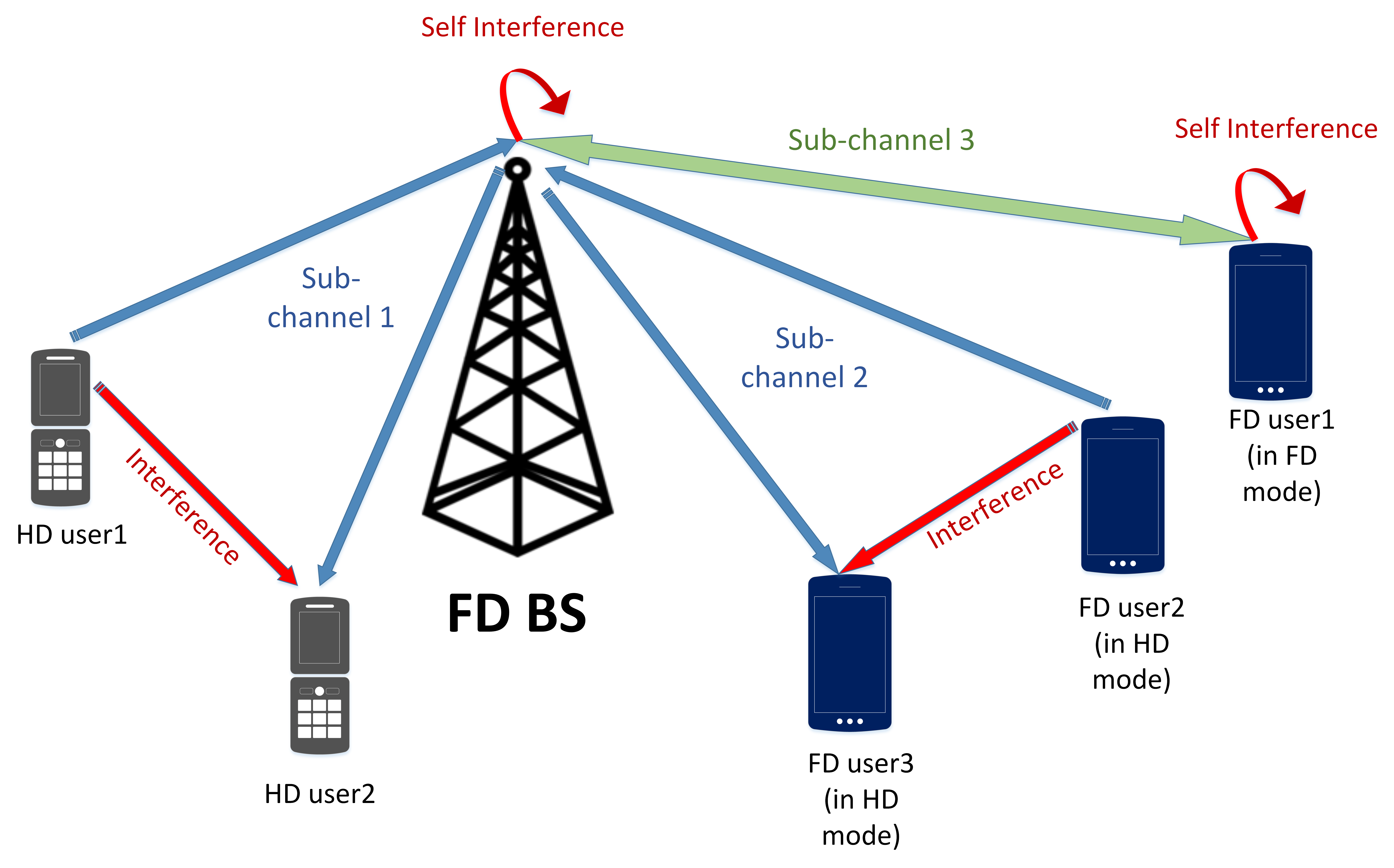
Figure 1: A single cell OFDMA full-duplex network that contains an imperfect full-duplex base-station and multiple half-duplex and full-duplex mobile nodes. Due to the full-duplex nature of this network, the base-station suffers from its self interference, and the uplink nodes cause interference to their co-channel downlink nodes.

We define the downlink weighted sum-rate as

$$R_{d}=\sum_{k=1}^{K}\sum_{n\in S_{k,d}}w_{k}\log\bigg{(}1+\frac{g_{k}(n)p_{k,d}(n)}{N_{k}+I_{k,j}(n)p_{j,u}(n)}\bigg{)}\vspace{-0mm}$$ (1)

And the uplink weighted sum-rate as

$$R_{u}=\sum_{j=1}^{K}\sum_{n\in S_{j,u}}v_{j}\log\bigg{(}1+\frac{g_{j}(n)p_{j,u}(n)}{N_{0}+\beta p_{k,d}(n)}\bigg{)}$$ (2)

The variables used in the above equations are introduced in Table I. We assume here that the channel is reciprocal, i.e., uplink and downlink channel gains are the same. We further assume that the receiver noise powers in different sub-channels are the same. The term $I_{k,j}(n)p_{j,u}(n)$ in (1) denotes the interference: When user $k$ is a FD device and both downlink and uplink of sub-channel $n$ are allocated to it $(j=k)$, $I_{k,j}(n)=\beta$, else $I_{k,j}(n)=g_{k,j}(n)$ is the channel gain between uplink user $j$ and downlink user $k$. We assume that the base-station knows all the channel gains, the noise powers, and the SI cancellation coefficient and weights assigned to the downlink and uplink of all users.

Let $P_{0}$ and $P_{k}$ denote the maximum available transmit power for the base-station and for user $k$, respectively. Then the proposed design optimization problem, denoted by P1, can be formulated as follows

TABLE I: Main Parameters and Variables

$w_{k}$	weight assigned to the downlink of user $k$
$v_{k}$	weight assigned to the uplink of user $k$
$p_{k,d}(n)$	transmission power from BS to user $k$ on sub-channel $n$
$p_{j,u}(n)$	transmission power from user $j$ to BS on sub-channel $n$
$N_{k}$	Gaussian noise variance at the receiver of user $k$
$N_{0}$	Gaussian noise variance at the base-station receiver
$S_{k,d}$	set of sub-channels allocated to user $k$ for downlink
$S_{j,u}$	set of sub-channels allocated to user $j$ for uplink
$\beta$	self-interference cancellation coefficient
$g_{k}(n)$	channel gain between BS and user $k$ on sub-channel $n$
$g_{k,j}(n)$	channel gain between users $j$ and $k$ on sub-channel $n$
$I_{k,j}(n)$	equal to $\beta$ when $j=k$, and to $g_{k,j}(n)$ otherwise
$P_{0}$	maximum available transmit power at BS
$P_{k}$	maximum available transmit power at user $k$

$$\textbf{{P}1}:\operatorname*{maximize}_{p_{k,d},p_{j,u},S_{j,u},S_{k,d},\forall k,j}\qquad R_{d}+R_{u}$$ (3)

$$\text{subject to }\sum_{k=1}^{K}\sum_{n\in S_{k,d}}p_{k,d}(n)\leq P_{0}$$ (4)

$$\sum_{n\in S_{j,u}}p_{j,u}(n)\leq P_{j}\quad\forall j$$ (5)

$$p_{j,u}(n),p_{k,d}(n)\geq 0\quad\forall j,k,n$$ (6)

$$S_{i,d}\cap S_{j,d}=\phi,S_{i,u}\cap S_{j,u}=\phi\quad\forall i\neq j$$ (7)

$$\cup_{j=1}^{K}\ S_{j,u}\subseteq\{1,2,...,N\},\cup_{k=1}^{K}\ S_{k,d}\subseteq\{1,2,...,N\}$$ (8)

$$S_{k,u}\cap S_{k,d}=\phi\quad\text{if user}\ k\ \text{is}\ \text{HD}$$ (9)

where (4) and (5) indicate the power constraint on the BS and the users, respectively. Constraint (6) shows the non-negativity feature of powers; (7) come from the fact that a sub-channel cannot be allocated to two distinct users simultaneously; (8) indicate that we have no more than $N$ sub-channels, and the last constraint accounts for the half-duplex nature of the HD users.

The general resource allocation problem presented is combinatorial in nature because of the channel allocation issue and addressing it together with power allocation in an optimal manner is challenging, especially as the number of users and sub-channels grow. Moreover, the non-convexity of the rate function makes the power allocation problem itself challenging even for a fixed sub-channel assignment. Here, we invoke a two step approximate solution. First, we determine the allocation of downlink and uplink sub-channels to users and then determine the transmit power of the users and the base-station on their allocated sub-channels. In other words, we first specify the sets $S_{k,d}$ and $S_{j,u}$ and then determine the variables $p_{j,u}(n)$, $p_{k,d}(n)$. In the next Section, we introduce our sub-channel allocation algorithm.

III Sub-channel Allocation

The sub-channel allocation problem, denoted by P2, can be formulated as follows

$$\textbf{{P}2}: \operatorname*{maximize}_{S_{j,u},S_{k,d}}\qquad R_{d}+R_{u}$$

subject to (7)-(11)

To solve the problem P2, we should first solve the following power allocation problem, denoted by P3, to maximize the weighted sum-rate in a single sub-channel and for a fixed pair of uplink and downlink users. Since a single sub-channel is being considered in P3, we have dropped the variable $n$ in the notation.

$$\textbf{{P}3}:\operatorname*{max}_{p_{k,d},p_{j,u}}L(p_{k,d},p_{j,u})= w_{k}\log(1+\frac{g_{k}p_{k,d}}{N_{k}+I_{k,j}p_{j,u}})+v_{j}\log(1+\frac{g_{j}p_{j,u}}{N_{0}+\beta p_{k,d}})$$

$$0\leq p_{k,d}\leq P_{max1}$$ (10)

$$0\leq p_{j,u}\leq P_{max2}$$ (11)

Here, $P_{max1}$ and $P_{max2}$ are the maximum allowable transmit powers.

Proposition 1.

For a fixed downlink user $k$ and uplink user $j$, the optimal pair of powers $(p_{k,d}^{*},p_{j,u}^{*})$ that optimizes P3 belongs to the following set.

$$\textbf{S}=\{(0,P_{max2}),(P_{max1},0),(P_{max1},P_{max2}), (p_{k,d}^{a},P_{max2}),(P_{max1},p_{j,u}^{a})\}$$

where

$$p_{k,d}^{a}=\frac{-B-\sqrt{B^{2}-4AC}}{2A},p_{j,u}^{a}=\frac{-E-\sqrt{E^{2}-4DF}}{2D}$$ (12)

and

$$A =w_{k}g_{k}\beta^{2},B=2w_{k}N_{0}g_{k}\beta+(w_{k}-v_{j})\beta g_{k}g_{j}p_{j,u}$$ (13)

$$C =w_{k}g_{k}N_{0}^{2}+w_{k}g_{k}g_{j}N_{0}p_{j,u}-v_{j}N_{k}g_{j}p_{j,u}\beta-v_{j}g_{j}\beta I_{k,j}p_{j,u}^{2}$$ (14)

$$D =v_{j}g_{j}I_{k,j}^{2},E=2v_{j}N_{k}g_{j}I_{k,j}+(v_{j}-w_{k})I_{k,j}g_{k}g_{j}p_{k,d}$$ (15)

$$F =v_{j}g_{j}N_{k}^{2}+v_{j}g_{k}g_{j}N_{k}p_{k,d}-w_{k}N_{0}g_{k}p_{k,d}I_{k,j}-w_{k}g_{k}\beta I_{k,j}p_{k,d}^{2}$$ (16)

Proof.

Computing the derivative with respect to $p_{k,d}$ and setting it to zero we have:

$$\frac{\partial L}{\partial p_{k,d}}=0\Longrightarrow Ap_{k,d}^{2}+Bp_{k,d}+C=0$$

where $A$, $B$ and $C$ are defined above. It is evident that $A\geq 0$, and if $w_{k}\geq v_{j}$ then $B\geq 0$. When $A,B\geq 0$ the above quadratic equation either has no zeros in $[0,P_{max1}]$ or has only one zero where the function changes sign from $-$ to $+$ indicating a local minimum for $L$. Therefore, in both cases the maximum is attained at a boundary point $0$ or $P_{max1}$. But when $w_{k}\leq v_{j}$, $B$ could be negative, and the smaller root of the quadratic equation $p_{k,d}^{a}$ could be positive. In this case, the maximum is attained at $P_{max1}$ or $p_{k,d}^{a}$. By similar analysis for $p_{j,u}$ one sees that if $v_{j}\geq w_{k}$ then the maximum is attained at a boundary point $0$ or $P_{max2}$ and when $w_{k}\geq v_{j}$ the maximum is attained at $P_{max2}$ or $p_{j,u}^{a}$. As a result, when $B\geq 0$ the optimal transmission powers belong to the following set,

$$P_{opt1}=\left\{(0,P_{max2}),(P_{max1},0),(P_{max1},P_{max2}),(P_{max1},p_{j,u}^{a})\right\}.$$

Otherwise, if $B<0$, they belong to the set below

$$P_{opt2}=\left\{(0,P_{max2}),(P_{max1},0),(P_{max1},P_{max2}),(p_{k,d}^{a},P_{max2})\right\}.$$

The cases $(0,p_{j,u}^{a})$ and $(p_{k,d}^{a},0)$ cannot be the optimal solutions of P3 , because they are dominated by $(0,P_{max2})$ and $(P_{max1},0)$ which give a larger $L$. Therefore, optimal powers could be found by checking the members of the set S and picking the one that corresponds to the largest $L$. ∎

Based on the above Proposition one can find the best uplink-downlink pair in each sub-channel by choosing the one with the largest value of $L$. This involves only $O(K^{2})$ operations. Now we can present our sub-channel allocation algorithm to solve Problem P2, in which we employ a sub-optimum power allocation scheme. First, for each sub-channel $n$, we find the best channel gain among all users and denote it by $\tilde{g}({n})=\operatorname*{arg\,max}_{k}g_{k}(n)$. Then, we sort the sub-channels based on the value of $\tilde{g}({n})$. In other words. we find a sub-channel permutation $\{a_{1},...,a_{N}\}$ such that $\tilde{g}({a_{1}})\geq\tilde{g}({a_{2}})\geq...\geq\tilde{g}({a_{N}})$. Then, starting from sub-channel $a_{1}$, we seek $k$ and $j$ that maximize $L$. At the first iteration, we set $P_{max1}=P_{0}$ , $P_{max2}=P_{k}$ and for iteration $l\geq 2$ set $P_{max1}=\frac{P_{0}}{d_{0}(l)}$ and $P_{max2}=\frac{P_{k}}{d_{k}(l)}$ where $d_{0}(l)$ and $d_{k}(l)$ indicate the number of sub-channels to be allocated to the BS’s downlink transmission and to user $k$’s uplink transmission, respectively, in the $l$th iteration. The proposed sub-channel allocation algorithm is summarized below.

Algorithm 1: Sub-channel Allocation Algorithm
1.for $n=1$ to $N$ do
2. $\tilde{g}({n})=\operatorname*{max}_{k}g_{k}(n)$
3.end for
4.Find a sub-channel permutation $\{a_{1},...,a_{N}\}$, $a_{i}\in\{1,...,N\}$, $a_{i}\neq a_{j}$ such that
$\tilde{g}({a_{1}})\geq\tilde{g}({a_{2}})\geq...\geq\tilde{g}({a_{N}})$
5. set $d_{k}(l)=1$ for $0\leq k\leq K$ and $1\leq l\leq N$
6.for $l=1$ to $N$ do
7. Set $P_{max1}=\dfrac{P_{0}}{d_{0}(l)}$ and $P_{max2}=\dfrac{P_{k}}{d_{k}(l)}\forall k$
8.  for $k=1$ to $K$ do
9.   for $j=1$ to $K$ (if $k$ is an HD user $j\neq k$)
10.   In sub-channel $a_{l}$ solve the problem P3
11.  end for
12. end for
13. Using the obtained optimal powers, find the best pair $(k^{*},j^{*})$ in the
sub-channel $a_{l}^{*}$ that has the largest value of $L$
14. $S_{j^{*},u}\leftarrow[{S_{j^{*},u},a_{l}}]$ , $S_{k^{*},d}\leftarrow[{S_{k^{*},d},a_{l}}]$
15. if $p_{k^{*}}\neq 0$ then $d_{0}(n)=d_{0}(n)+1$;
16. if $p_{j^{*}}\neq 0$ then $d_{j^{*}}(n)=d_{j^{*}}(n)+1$;
17.end for

The complexity of finding the best user in each sub-channel is $O(K)$ and for $N$ sub-channels is $O(KN)$. Similarly, the complexity of finding the best pair in each sub-channel is $O(K^{2})$ and doing so for $N$ sub-channels requires $O(NK^{2})$ operations. Since the complexity of sorting $N$ values is $O(N\log N)$, then the overall computational complexity of the proposed sub-channel allocation algorithm is $O(N\log N+NK^{2})$.

IV Power Allocation

The power allocation problem, denoted by P4, can be formulated as follows

$$\textbf{{P}4}: \operatorname*{maximize}_{p_{k,d},p_{j,u}}\qquad R_{d}+R_{u}$$

subject to (4)-(6)

Due to the interference terms, the power allocation problem is non-convex. Here, we use the “difference of two concave functions/sets” (DC) programming technique [17] to convexify this problem. In this procedure, the non-concave objective function is expressed as the difference of two concave functions, and the discounted term is approximated by its first order Taylor series. Hence, the objective becomes concave and can be maximized by known convex optimization methods. This procedure runs iteratively, and after each iteration the optimal solution serves as an initial point for the next iteration until the improvement diminishes in iterations. In [18], the DC approach is used to formulate optimized power allocation in a multiuser interference channel, and in [19], the DC optimization method is used to optimize the energy efficiency of an OFDMA device to device network. Here, we rewrite the objective function of P4 in DC form as follows

$$\operatorname*{max}_{\mathbf{p}}\quad f(\mathbf{p})-h(\mathbf{p})$$

$$f(\mathbf{p}) =\sum_{k=1}^{K}\sum_{n\in S_{k,d}}w_{k}\log(N_{k}+I_{k,j}(n)p_{j,u}(n)+g_{k}(n)p_{k,d}(n))$$

$$+\sum_{j=1}^{K}\sum_{n\in S_{j,u}}v_{j}\log(N_{0}+\beta p_{k,d}(n)+g_{j}(n)p_{j,u}(n))$$

$$h(\mathbf{p}) =\sum_{k=1}^{K}\sum_{n\in S_{k,d}}w_{k}\log(N_{k}+I_{k,j}(n)p_{j,u}(n))$$

$$+\sum_{j=1}^{K}\sum_{n\in S_{j,u}}v_{j}\log(N_{0}+\beta p_{k,d}(n))$$

where

$$\mathbf{p}=[p_{k_{1},d}(1),...,p_{k_{N},d}(N),p_{j_{1},u}(1),,...,p_{j_{N},u}(N)]^{T}$$

is the downlink and uplink transmitted power vector, and $k_{i}$ and $j_{i}$ denote the uplink and downlink users that are selected for the $i$th sub-channel after the sub-channel allocation phase. Now, the objective $f(\mathbf{p})-h(\mathbf{p})$ is a DC function. To write the Taylor series of the discounted function $h(\mathbf{p}$), we need its gradient, that can be easily derived as follows.

$$\nabla h(\mathbf{p})=\bigg{[}\frac{u_{j_{1}}\beta}{\ln(2)}\frac{1}{N_{0}+\beta p_{k_{1},d}(1))},...,\frac{u_{j_{N}}\beta}{\ln(2)}\frac{N}{N_{0}+\beta p_{k_{N},d}(N))},$$

$$\frac{w_{k_{1}}I_{k_{1},j_{1}}(1)}{\ln(2)}\frac{1}{N_{k_{1}}+I_{k_{1},j_{1}}(1)p_{j_{1},u}(1))},...,$$

$$\frac{w_{k_{N}}I_{k_{N},j_{N}}(N)}{\ln(2)}\frac{1}{N_{k_{N}}+I_{k_{N},j_{N}}(N)p_{j_{N},u}(N))}\bigg{]}^{T}$$

To make the problem convex, $h(\mathbf{p})$ is approximated with its first order approximation $h(\mathbf{p}^{(t)})+\nabla h^{T}(\mathbf{p}^{(t)})(\mathbf{p}-\mathbf{p}^{(t)})$ at point $\mathbf{p}^{(t)}$. We start from a feasible $\mathbf{p}^{(0)}$ at the first iteration, and $\mathbf{p}^{(t+1)}$ at the $t$th iteration is generated as the optimal solution of the following convex program

$$\mathbf{p}^{(t+1)}=\operatorname*{argmax}_{\mathbf{p}}\quad f(\mathbf{p})-h(\mathbf{p}^{(t)})-\nabla h^{T}(\mathbf{p}^{(t)})(\mathbf{p}-\mathbf{p}^{(t)})$$

$$\text{subject to }\ (4)-(6)$$

Since $h(\mathbf{p})$ is a concave function, its gradient is also its super gradient so we have

$$h(\mathbf{p})\leq h(\mathbf{p}^{(t)})+\nabla h^{T}(\mathbf{p}^{(t)})(\mathbf{p}-\mathbf{p}^{(t)}),\quad\quad\forall\mathbf{p}$$

and we can deduce

$$h(\mathbf{p}^{(t+1)})\leq h(\mathbf{p}^{(t)})+\nabla h^{T}(\mathbf{p}^{(t)})(\mathbf{p}^{(t+1)}-\mathbf{p}^{(t)}).$$

Then it can be proved that in each iteration the solution of problem P4 is improved as follows

$$f(\mathbf{p}^{(t+1)})-h(\mathbf{p}^{(t+1)})\geq$$

$$f(\mathbf{p}^{(t+1)})-h(\mathbf{p}^{(t)})-\nabla h^{T}(\mathbf{p}^{(t)})(\mathbf{p}^{(t+1)}-\mathbf{p}^{(t)})$$

$$=\operatorname*{max}_{\mathbf{p}}\quad f(\mathbf{p})-h(\mathbf{p}^{(t)})-\nabla h^{T}(\mathbf{p}^{(t)})(\mathbf{p}-\mathbf{p}^{(t)})$$

$$\geq f(\mathbf{p}^{(t)})-h(\mathbf{p}^{(t)})-\nabla h^{T}(\mathbf{p}^{(t)})(\mathbf{p}^{(t)}-\mathbf{p}^{(t)})$$

$$=f(\mathbf{p}^{(t)})-h(\mathbf{p}^{(t)}).$$

According to the above equations, the objective value after each iteration is either unchanged or improved and since the constraint set is compact it can be concluded that the above DC approach converges to a local maximum.

V Analyzing Self-Interference Cancellation Coefficient Threshold

In [20], through simulations it has been observed that in a network that contains an imperfect FD BS and some imperfect FD and HD users, when the self-interference cancellation coefficient is larger than a specified threshold, there is no difference between the throughput of an all HD user network and an all FD user network. Here we wish to analyze this threshold.
Recall that in FD networks there are four possible types of connections in a given sub-channel:

1. HD downlink

2. HD uplink

3. Joint downlink and uplink for two distinct users over an FD BS

4. A full-duplex bidirectional connection between an FD user and an FD BS

Employing an FD user in a cell with an FD capable BS can increase the throughput when the 4th case is more appealing than the other cases in at least one sub-channel. Considering sub-channel $n$, we assume that user $d$ is the best downlink user, user $u$ is the best uplink user, users $a$ and $b$ are the best downlink and uplink pair, and user $f$ is the best FD node for FD communication with the BS. Here the best user, is the user who gives the highest weighted rate with the same power than the rest. The rate of the four previous cases are presented below (we drop the sub-channel index $n$ for simplicity)

$$R_{d}=w_{d}\log\bigg{(}1+\frac{g_{d}p_{Bd}}{N_{d}}\bigg{)}$$ (17)

$$R_{u}=v_{u}\log\bigg{(}1+\frac{g_{u}p_{uB}}{N_{0}}\bigg{)}$$ (18)

$$R_{du}= w_{a}\log\bigg{(}1+\frac{g_{a}p_{Ba}}{N_{a}+g_{ba}p_{bB}}\bigg{)}+v_{b}\log\bigg{(}1+\frac{g_{b}p_{bB}}{N_{0}+\beta p_{Ba}}\bigg{)}$$ (19)

$$R_{f}=w_{f}\log\bigg{(}1+\frac{g_{f}p_{Bf}}{N_{f}+\beta p_{fB}}\bigg{)}+v_{f}\log\bigg{(}1+\frac{g_{f}p_{fB}}{N_{0}+\beta p_{Bf}}\bigg{)}$$ (20)

where, $p_{Bx}$ and $p_{yB}$ are the transmission powers form BS to user $x$ and from user $y$ to the BS, respectively. The other variables were introduced in Table I. In short, using an FD user in the network could be beneficial when these conditions hold in at least one sub-channel:

$$R_{f}>R_{d}$$ (21)

$$R_{f}>R_{u}$$ (22)

$$R_{f}>R_{du}.$$ (23)

Since we wish to focus on parameter $\beta$, and to avoid dealing with other parameters, we introduce some simplifications. First, we assume the sum rate case where, $w_{d}=v_{u}=w_{a}=w_{f}=v_{b}=v_{f}=1$. Second, we assume that the noise powers at the BS and at the users are the same. Third, we assume that the transmission power from the BS to all users is the same and is equal to the average BS power, i.e., $p_{Bd}=p_{Ba}=p_{Bb}=p_{Bf}=\frac{P_{0}}{N}=P_{BS}$. Fourth, we assume that the transmission powers from different users to the BS are the same and are equal to the average user power, i.e., $p_{uB}=p_{bB}=p_{fB}=\frac{KP_{K}}{N}=P_{user}$. Fifth, the channel gains $g_{d}$, $g_{u}$, $g_{f}$, $g_{a}$, $g_{b}$, $g_{ba}$ are random variables and in the sum rate case the best downlink user, the best uplink user and the best FD user are all the same $g_{d}=g_{u}=g_{f}=g_{max}$, because the channel is reciprocal and the user with maximum channel gain is selected for all of these three cases. If we assume that the number of users in the network is $K$, then random variable $g_{max}$ can be defined as: $g_{max}=\text{max}\left\{g_{1},g_{2},...,g_{K}\right\}$, where $g_{i}$ is the random channel gain between the BS and the user $i$, that itself is a multiplication of an exponential random variable, $e_{i}$, with unit power and a path loss random variable $l_{i}$ that depends on the path loss model and the distance $d_{i}$ between the BS and the $i$th user whose pdf is shown by $f_{D_{i}}(d_{i})=\frac{2d_{i}}{R_{cell}^{2}}$ (for $0<d_{i}<R_{cell}$). We assume $g_{ab}$ is a random channel gain between two users $a$ and $b$ which are distributed uniformly in a circle with radius $R_{cell}$.We also assume that $g_{a}$ and $g_{b}$ are the maximum and the second maximum channel gain between $K$ users.

Due to the randomness of the channel gains, $\beta$ itself is a random variable and here we wish to derive its distribution. According to conditions (21) - (23), we have:

1. The FD rate should be bigger than the HD downlink rate, so we have:

   $$\log(1+\frac{g_{f}P_{BS}}{N_{0}+\beta P_{user}})+\log(1+\frac{g_{f}P_{user}}{N_{0}+\beta P_{BS}})>\log(1+\frac{g_{d}P_{BS}}{N_{0}})$$

   After some manipulations, this is reduced to the inequality $a_{1}\beta^{2}+b_{1}\beta-c_{1}<0$, where:

   $$a_{1} =g_{d}P^{2}_{BS}P_{user}$$ (24)

   $$b_{1} =N_{0}g_{f}P_{user}(P_{BS}-P_{user})$$ (25)

   $$c_{1} =N_{0}^{2}g_{f}P_{user}+N_{0}g^{2}_{f}P_{BS}P_{user}$$ (26)

   which holds for $0<\beta<\frac{-b_{1}+\sqrt{b_{1}^{2}+4a_{1}c_{1}}}{2a_{1}}$. Therefore, due to condition (21) $\beta_{1}=\frac{-b_{1}+\sqrt{b_{1}^{2}+4a_{1}c_{1}}}{2a_{1}}$.

2. By writing the condition (22) and doing the same procedure as the previous part we arrive at inequality $a_{2}\beta^{2}+b_{2}\beta-c_{2}<0$ where:

   $$a_{2} =g_{u}P^{2}_{user}P_{BS}$$ (27)

   $$b_{2} =N_{0}g_{u}P_{BS}(P_{user}-P_{BS})$$ (28)

   $$c_{2} =N_{0}^{2}g_{f}P_{BS}+N_{0}g^{2}_{f}P_{BS}P_{user}$$ (29)

   which holds for $0<\beta<\frac{-b_{2}+\sqrt{b_{2}^{2}+4a_{2}c_{2}}}{2a_{2}}$. Therefore, according to (22) $\beta_{2}=\frac{-b_{2}+\sqrt{b_{2}^{2}+4a_{2}c_{2}}}{2a_{2}}$.

3. By writing the condition (23) and doing the same procedure as the previous parts we arrive at the inequality $a_{3}\beta^{3}+b_{3}\beta^{2}+c_{3}\beta+d_{3}<0$, where:

   $$a_{3}=P_{BS}^{3}P_{user}g_{a}$$ (30)

   $$b_{3}=P_{user}^{2}P_{BS}g_{b}N_{0}+P_{user}^{3}P_{BS}g_{b}g_{ab}+P_{user}^{2}P_{BS}^{2}g_{b}g_{a}+$$

   $$P_{BS}^{2}P_{user}g_{a}N_{0}+P_{BS}^{3}g_{a}N_{0}-P_{user}^{2}P_{BS}g_{f}N_{0}-$$

   $$P_{BS}^{3}g_{f}N_{0}-g_{f}P_{BS}^{3}P_{user}g_{ab}-P_{user}^{3}P_{BS}g_{f}g_{ab}$$ (31)

   $$c_{3}=P_{user}^{2}P_{B}Sg_{b}N_{0}g_{a}+P_{user}^{3}g_{ab}N_{0}g_{b}+P_{user}^{2}N_{0}^{2}g_{b}+$$

   $$P_{user}P_{BS}N_{0}^{2}g_{a}+P_{BS}^{2}P_{user}g_{b}N_{0}g_{a}+P_{user}^{2}P_{BS}g_{b}N_{0}g_{ab}+$$

   $$N_{0}^{2}P_{BS}g_{b}P_{user}+2N_{0}^{2}P_{BS}^{2}g_{a}-P_{user}^{3}g_{f}g_{ab}N_{0}-$$

   $$P_{BS}^{2}g_{f}g_{ab}N_{0}P_{user}-P_{BS}^{2}g_{f}^{2}N_{0}P_{user}-N_{0}^{2}g_{f}P_{BS}P_{user}-$$

   $$2P_{BS}^{2}N_{0}^{2}g_{f}-P_{user}^{2}N_{0}^{2}g_{f}-P_{BS}^{2}P_{user}g_{f}g_{ab}N_{0}-$$

   $$P_{BS}g_{ab}P_{user}^{2}N_{0}g_{f}-g_{f}^{2}P_{BS}^{2}P_{user}^{2}g_{ab}$$ (32)

   $$d_{3}=P_{BS}N_{0}^{3}g_{a}+P_{user}N_{0}^{3}g_{b}+P_{user}^{2}N_{0}^{2}g_{b}g_{ab}+$$

   $$P_{user}P_{BS}N_{0}^{2}g_{b}g_{a}-P_{user}^{2}N_{0}g_{f}^{2}g_{ab}P_{BS}-P_{user}^{2}g_{f}N_{0}^{2}g_{ab}-$$

   $$P_{user}g_{f}N_{0}^{2})g_{ab}P_{BS}-P_{user}g_{f}^{2}N_{0}^{2}P_{BS}-P_{user}g_{f}N_{0}^{3}-$$

   $$P_{BS}g_{f}N_{0}^{3}$$ (33)

   The above cubic function has the following three roots:

   $$x_{1}= A+B-\frac{b}{3}$$ (34)

   $$x_{2}= \frac{-1}{2}(A+B)+\frac{i\sqrt{3}}{2}(A-B)-\frac{b}{3}$$ (35)

   $$x_{3}= \frac{-1}{2}(A+B)-\frac{i\sqrt{3}}{2}(A-B)-\frac{b}{3}$$ (36)

   where

   $$A= \sqrt[3]{\frac{-q}{2}+\sqrt{\frac{q^{2}}{4}+\frac{p^{3}}{27}}}$$ (37)

   $$B= \sqrt[3]{\frac{-q}{2}-\sqrt{\frac{q^{2}}{4}+\frac{p^{3}}{27}}}$$ (38)

   $$p= \frac{-b^{2}}{3}+c$$ (39)

   $$q= \frac{2b^{3}}{27}-\frac{bc}{3}+d$$ (40)

   $$b=\frac{b_{3}}{a_{3}},\quad c=\frac{c_{3}}{a_{3}},\quad d=\frac{d_{3}}{a_{3}}$$ (41)

   It is evident that $a_{3}\geq 0$. Also, it can be shown that the value of $d_{3}$ is always negative, therefore, it is deduced that the cubic function has at least one positive real root. Therefore, due to the condition (23), $\beta_{3}=\min\left\{R(x_{1}),R(x_{2}),R(x_{3})\right\}$ is the smallest positive real root of this cubic function, where $R(x)$ is given by:

   $$R(x)=\left\{\begin{array}[]{lr}x&\mbox{if }x\mbox{ is real and positive}\\ \infty&\mbox{Otherwise}.\end{array}\right.$$

   Finally, we arrive at the following proposition:

   Proposition 2.

   For a wireless cell with an FD BS and users with imperfect SI cancellation factor $\beta$, FD operation is advantageous from the perspective of the network throughput performance if $\beta<\beta_{Threshold}=\min\left\{\beta_{1},\beta_{2},\beta_{3}\right\}$.

In Section VII, we will compare the outcome of this analysis with simulation results.

VI Two-Tier Heterogeneous Full Duplex Network

In this section, we consider a two-tier heterogeneous full-duplex OFDMA network. This system includes a macrocell FD BS and multiple femto cell FD BSs along with their associated HD and FD users. Our goal is to maximize the uplink and downlik weighted sum rate of femto cell users while provisioning for the macrocell user’s uplink and downlink data rate. Assume that the numbers of femto cells and available sub-channels are $M_{f}$ and $N$, respectively, and the number of users related to the $m$th BS is $K_{m}$. We denote the set of all BSs as $\Omega=\{0,1,2,...,M_{f}\}$, where the macro BS is indexed by 0. The variables used in the following equations are summarized in Table II.

The downlink rate in cell $m$ is given by:

$$R_{d,m}=\sum_{k=1}^{K_{m}}\sum_{n\in S_{k,d,m}}w_{k,m}\log\bigg{(}1+$$

$$\frac{g_{k,m}(n)p_{k,d,m}(n)}{N_{k,m}+\sum_{j=1}^{K_{m}}I_{k,j,m}(n)p_{j,u,m}(n)+DIC_{m,k}(n)+UIC_{m,k}(n)}\bigg{)}$$ (42)

where $DIC_{m,k}(n)$ and $UIC_{m,k}(n)$ are the downlink and uplink inter-cell interference on sub-channel $n$ in the $m$th cell for user $k$, i.e.:

$$DIC_{m,k}(n)=\sum_{m^{{}^{\prime}}\in\Omega\text{\textbackslash}\{m\}}g_{k,m,m^{{}^{\prime}}}(n)p_{d,m^{{}^{\prime}}}(n)$$ (43)

$$UIC_{m,k}(n)=\sum_{m^{{}^{\prime}}\in\Omega\text{\textbackslash}\{m\}}\sum_{j=1}^{K_{m^{{}^{\prime}}}}g_{k,m,j,{m^{{}^{\prime}}}}(n)p_{j,u,m^{{}^{\prime}}}(n)$$ (44)

Similarly the uplink rate in cell $m$ is given by:

$$R_{u,m}=\sum_{j=1}^{K_{m}}\sum_{n\in S_{j,u,m}}v_{j}\log\bigg{(}1+$$

$$\frac{g_{j,m}(n)p_{j,u,m}(n)}{N_{m}+\beta\sum_{k=1}^{K_{m}}p_{k,d,m}(n)+DIC_{m}(n)+UIC_{m}(n)}\bigg{)}$$ (45)

where $DIC_{m}(n)$ and $UIC_{m}(n)$ are the downlink and uplink inter-cell interference on sub-channel $n$ at the $m$th BS, i.e.:

$$DIC_{m}(n)=\sum_{m^{{}^{\prime}}\in\Omega\text{\textbackslash}\{m\}}g_{m,m^{{}^{\prime}}}(n)p_{d,m^{{}^{\prime}}}(n)$$ (46)

$$UIC_{m}(n)=\sum_{m^{{}^{\prime}}\in\Omega\text{\textbackslash}\{m\}}\sum_{j=1}^{K_{m^{{}^{\prime}}}}g_{j,{m^{{}^{\prime}}},m}(n)p_{j,u,m^{{}^{\prime}}}(n)$$ (47)

TABLE II: Key Variables For The Heterogeneous Network

$w_{k,m}$	weight assigned to the downlink of user $k$ in the $m$th cell
$v_{j,m}$	weight assigned to the uplink of user $j$ in the $m$th cell
$p_{k,d,m}(n)$	downlink transmission power from the BS to user $k$ on sub-channel $n$ in the $m$th cell
$p_{j,u,m}(n)$	uplink transmission power from user $j$ to the BS on sub-channel $n$ in the $m$th cell
$p_{d,m^{{}^{\prime}}}(n)$	downlink transmission power from the $m^{{}^{\prime}}$th BS on sub-channel $n$
$g_{k,m,m^{{}^{\prime}}}(n)$	channel gain between user $k$ in the $m$th cell and the $m^{{}^{\prime}}$th BS on sub-channel $n$
$g_{k,m,j,{m^{{}^{\prime}}}}(n)$	channel gain between user $k$ in the $m$th cell and user $j$ in the $m^{{}^{\prime}}$th cell on sub-channel $n$
$g_{k,m}(n)$	channel gain between the BS and user $k$ on sub-channel $n$ in the $m$th cell
$g_{m,m^{{}^{\prime}}}(n)$	channel gain between the $m$th BS and the $m^{{}^{\prime}}$th BS on sub-channel $n$
$N_{k,m}$	Gaussian noise variance at the receiver of user $k$ in the $m$th cell
$N_{m}$	Gaussian noise variance at the $m$th base-station receiver
$S_{k,d,m}$	set of sub-channels allocated to user $k$ for downlink transmission in the $m$th cell
$S_{j,u,m}$	set of sub-channels allocated to user $j$ for uplink transmission in the $m$th cell
$\beta$	self-interference cancellation coefficient
$I_{k,j,m}(n)$	equal to $\beta$ when $j=k$, and to $g_{k,m,j,{m}}(n)$ otherwise
$P^{BS}_{m}$	maximum available transmit power at the $m$th BS
$P_{k,m}$	maximum available transmit power at user $k$ in the $m$th cell
$R_{mind}$	minimum required downlink rate for the macrocell
$R_{minu}$	minimum required uplink rate for the macrocell

The optimization problem for the heterogeneous network can be formulated as follows:

$$\textbf{{P}}_{\textbf{Het}}:\operatorname*{Maximize}_{p_{k,d,m},p_{j,u,m},S_{j,u,m},S_{k,d,m}}\qquad\sum_{m=1}^{M_{f}}R_{d,m}+R_{u,m}$$ (48)

$$\text{Subject to }\sum_{k=1}^{K_{m}}\sum_{n\in S_{k,d,m}}p_{k,d,m}(n)\leq P^{BS}_{m}\quad\forall m$$ (49)

$$\sum_{n\in S_{j,u,m}}p_{j,u,m}(n)\leq P_{j,m}\quad\forall j,m$$ (50)

$$R_{d,0}\geq R_{mind},\ R_{u,0}\geq R_{minu}$$ (51)

$$p_{j,u,m}(n),p_{k,d,m}(n)\geq 0\quad\forall j,k,n,m$$ (52)

$$S_{i,d,m}\cap S_{j,d,m}=\phi,\ S_{i,u,m}\cap S_{j,u,m}=\phi\quad\forall i\neq j,\forall m$$ (53)

$$\cup_{j=1}^{K_{m}}\ S_{j,u,m}\subseteq\{1,2,...,N\},\ \cup_{k=1}^{K_{m}}\ S_{k,d,m}\subseteq\{1,2,...,N\}\quad\forall m$$ (54)

$$S_{k,u,m}\cap S_{k,d,m}=\phi\quad\text{if user}\ k\ \text{is}\ \text{HD}\quad\forall m$$ (55)

where (49) and (50) indicate the power constraint on the BSs and the users, respectively; (51) is the minimum downlink and uplink rate constraints for the macrocell users. The constraint (52) shows the non-negativity of transmission powers; (53) comes from the fact that a sub-channel cannot be allocated to two distinct users simultaneously; (54) indicates that we have no more than $N$ sub-channels, and the last constraint accounts for the half-duplex nature of the HD users.

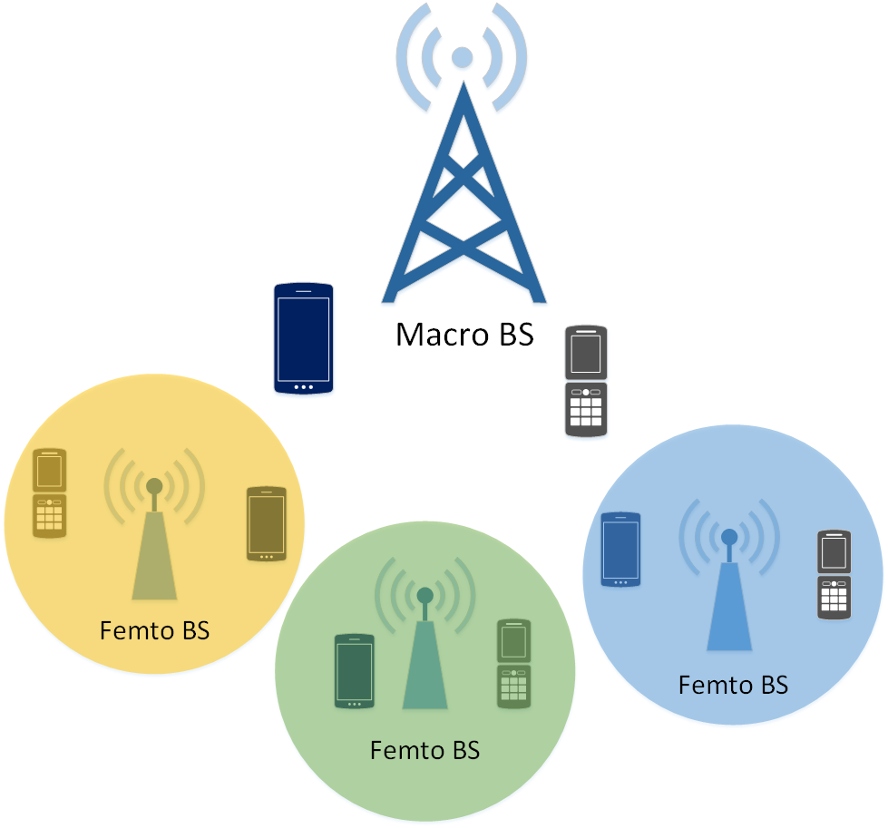
Figure 2: A two-tier heterogeneous OFDMA full-duplex network that contains an imperfect full-duplex macro base-station and multiple femto cell BSs and their associated users.

To address this problem, we propose a scheme which optimizes power allocation and sub-channel assignment in an iterative manner. At the beginning of each iteration $t$, we find the proper sub-channel assignment $\mathbf{S}[t]$ for the power allocation obtained from the last iteration $\mathbf{P}[t-1]$. Then for this $\mathbf{S}[t]$, we find the optimal power allocation. We repeat the process in all subsequent iterations until no further noticeable improvement is observed, i.e.:

$$\mathbf{S}[0]\longrightarrow\mathbf{P}[0]\longrightarrow\cdots\cdots\longrightarrow\mathbf{S}[t]\longrightarrow\mathbf{P}[t]$$

At the first iteration for sub-channel allocation, in each femto cell, sub-channels are allocated based on Algorithm 1 in Section III without considering the inter-cell interference. At the macro cell, since uplink-downlink rate constraints are to be satisfied, additional considerations are required. Algorithm 2 presents a solution for the rate-constrainted sub-channel allocation. Depending on whether $R_{mind}$ or $R_{minu}$ is larger, the algorithm allocates a downlink or uplink sub-channel and then the estimated resulting rate of the new added sub-channel is subtracted from the required minimum rate. This procedure is repeated until both $R_{mind}$ and $R_{minu}$ become equal or less than zero. In this case, a sufficient number of sub-channels has been allocated to uplink and downlink users in order to satisfy the rate constraints. After that, the algorithm switches to the one without the rate constraint.

Algorithm 2: Sub-channel Allocation Algorithm with Rate Constraint
1.for $n=1$ to $N$ do
2. $\tilde{g}({n})=\operatorname*{max}_{k}g_{k}(n)$
3.end for
4.Find a sub-channel permutation $\{a_{1},...,a_{N}\}$, $a_{i}\in\{1,...,N\}$, $a_{i}\neq a_{j}$ such that
$\tilde{g}({a_{1}})\geq\tilde{g}({a_{2}})\geq...\geq\tilde{g}({a_{N}})$
5. set $d_{k}(l)=1$ for $0\leq k\leq K$ and $1\leq l\leq N$
6.for $l=1$ to $N$ do
7. Set $P_{max1}=\dfrac{P_{0}}{d_{0}(l)}$ and $P_{max2}=\dfrac{P_{k}}{d_{k}(l)}\forall k$
8. if($(R_{mind}\geq 0$) and $(R_{mind}\geq R_{minu})$ )
begin
9.  In sub-channel $a_{l}$ find the best downlink user $k^{*}$
10.  $R_{mind}\longleftarrow R_{mind}-L(\frac{P_{0}}{d_{0}(l)},0)$
11.  $S_{k^{*},d}\leftarrow[{S_{k^{*},d},a_{l}}]$ and $d_{0}(n)=d_{0}(n)+1$;
end
12. elseif($(R_{minu}\geq 0)$ and ($R_{minu}\geq R_{mind}$))
begin
13.  In sub-channel $a_{l}$ find the best uplink user $j^{*}$
14.  $R_{minu}\longleftarrow R_{minu}-L(0,\frac{P_{j^{*}}}{d_{j^{*}}(l)})$
15.  $S_{j^{*},u}\leftarrow[{S_{j^{*},u},a_{l}}]$ and $d_{j^{*}}(l)=d_{j^{*}}(l)+1$;
end
16.  else
begin
17.  for $k=1$ to $K$ do
18.   for $j=1$ to $K$ (if $k$ is an HD user $j\neq k$)
19.   In sub-channel $a_{l}$ solve the problem P3
20.  end for
21. end for
22. Using the obtained optimal powers, find the best pair $(k^{*},j^{*})$ in the
sub-channel $a_{l}^{*}$ that has the largest value of $L$
23. $S_{j^{*},u}\leftarrow[{S_{j^{*},u},a_{l}}]$ , $S_{k^{*},d}\leftarrow[{S_{k^{*},d},a_{l}}]$
24. if $p_{k^{*}}\neq 0$ then $d_{0}(n)=d_{0}(n)+1$;
25. if $p_{j^{*}}\neq 0$ then $d_{j^{*}}(n)=d_{j^{*}}(n)+1$;
end
26.end for

After sub-channel allocation at the first iteration, we perform power allocation by using the DC approach as described in Section IV in order to convexify the objective function and the rate constraints. Then, for the next iterations, we perform sub-channel allocation by considering the inter-cell interference. To choose the best pair in each cell we use Proposition 1 in Section III. For a heterogeneous network, where $N_{k}$ is replaced by $N_{k}+DIC_{m,k}(n)+UIC_{m,k}(n)$ because in addition to Gaussian noise at the $k$th user we should take into account the uplink and downlnk interference from other cells. Similarly, because of the uplink and downlink interference at the BS we replace $N_{0}$ with $N_{0}+DIC_{m}(n)+UIC_{m}(n)$. The proof of convergence of power iterations is the same as in Section IV. For the sub-channel iterations, as many interfering nodes exist, the mathematical proof of convergence is intractable, but simulation results show that it converges to a local maximum.

VII Simulation Results

In this Section, we evaluate the proposed resource allocation scheme for OFDMA networks with half-duplex and imperfect full-duplex nodes. We assume a time-slotted system, where nodes are uniformly distributed within a given cell radius. Table III presents the details of the indoor and outdoor simulation setup and channel models for the single cell network. In addition to the path loss, a Rayleigh block fading channel model with unit average power is considered. The channel gains remain constant in each time slot and vary independently from one time slot to the next.

TABLE III: simulation parameters

PARAMETER	VALUE
Maximum BS Power (outdoor)	$43$ dBm
Maximum BS Power (indoor)	$24$ dBm
Maximum UE Power $(P_{k})$	$23$ dBm
Thermal Noise Density	$-170$ dBm/Hz
Number of Sub-channels $N$	$64$
Total Bandwidth	$10$ MHz
Sub-channel Bandwidth	$150$ KHz
Cell Radius (outdoor)	$1$ km
Cell Radius (indoor)	$20$ m
Center Frequency	$2$ GHz
BS to UE Path Loss (outdoor)	urban Hata model with parameters $h_{m}=1.5$ m, $h_{B}=30$ m
UE to UE Path Loss (outdoor)	urban Hata model with parameters $h_{m}=1.5$ m, $h_{B}=1.5$ m
Path Loss Model (indoor)	ITU model for indoor attenuation with parameters N= $22$, $p_{f}(n)=9$

For comparison of different cases in a single cell network, we consider six schemes: (i) An HD uplink system (HD-U), (ii) An HD downlink system (HD-D), (iii) a system that includes an FD BS and HD users (FD-HD), (iv) a system that contains an FD BS and FD users (FD-FD), (v) an upper bound which is the HD uplink rate plus the HD downlink rate; (vi) a Hybrid HD scheme (HHD), in which a hybrid HD BS could transmit data to downlink users and receive data from uplink users simultaneously in different sub-channels. For the HD-D case, each sub-channel is allocated to the user with the best weighted channel SNR, and multi-level water filling [21] is applied for power allocation. For the sub-channel assignment of the HD-U scheme the $SOA1\>4B\>5A$ method presented in [22] is used, and for power allocation each user performs water filling in its dedicated sub-channels. In the HHD scheme, we use the proposed sub-channel allocation algorithm by changing the set $P_{opt}$ to:

$$P_{opt}=\left\{(0,P_{max2}),(P_{max1},0)\right\}$$

and perform multi-level water filling and water filling for the power allocation in the selected downlink and uplink sub-channels, respectively.

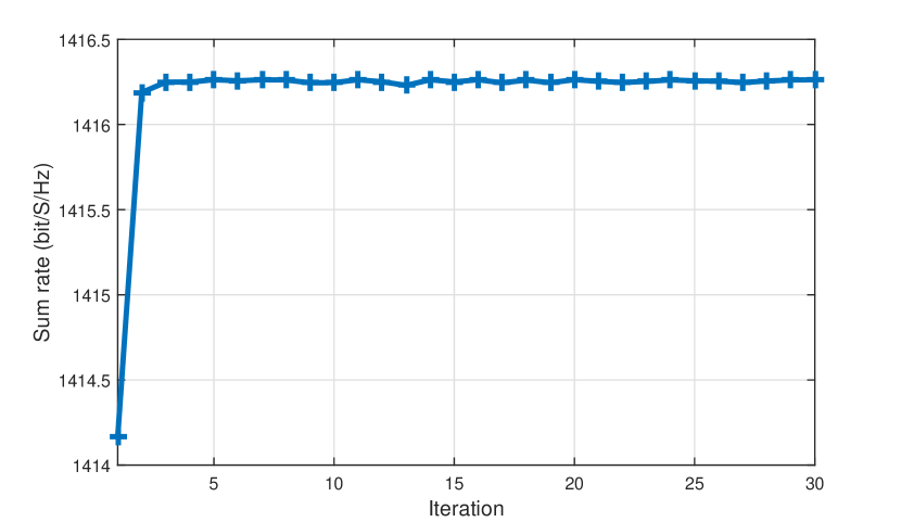
Figure 3: Convergence behavior of the proposed algorithm. Here $\beta=10^{-6}$ and other simulation parameters are the same as in the outdoor case.

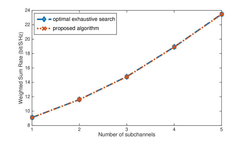
Figure 4: Performance comparison of the proposed algorithm with optimal exhaustive search in a small network.

Fig. 4 illustrates the convergence of the proposed resource allocation scheme in a single cell OFDMA network with 10 HD nodes and 10 imperfect FD nodes. As can be seen, the sum-rate converges in just a few iterations.

Fig. 4 compares the proposed algorithm with the optimal exhaustive search solution. Due to the high computational complexity of exhaustive search, only a small network with one HD and one FD user and a small number of sub-channels can be considered. Uplink and downlink weight vectors are assumed to be $\mathbf{u}=[1/3,2/3]^{T}$ and $\mathbf{w}=[2/3,1/3]^{T}$ respectively, and the SI cancellation coefficient is set to $\beta=-90$ dB. Simulation results show that, at least for small size networks, our proposed algorithm achieves the performance of the optimal exhaustive search.

Fig. 6 shows the sum-rate of the different schemes in the outdoor scenario with perfect SI cancellation ($\beta=0$). It can be seen that when the BS and all nodes are perfect FD devices the upper-bound could be attained, and when the nodes are HD but the BS is FD the sum-rate is still bigger than the cases with HD BS, but it can not reach the upper-bound because of inter-node interference.

Fig. 6 shows the sum-rate of the six presented schemes in an indoor scenario. If we compare the outdoor and indoor scenarios we find that using an FD BS in an outdoor environment has much larger gain than using it in an indoor case. This result is intuitive because in the outdoor environment the distances between nodes are larger, and hence the inter-node interference is smaller. As a result, the FD BS could work in FD mode in more sub-channels, which helps increase the network throughput more significantly.

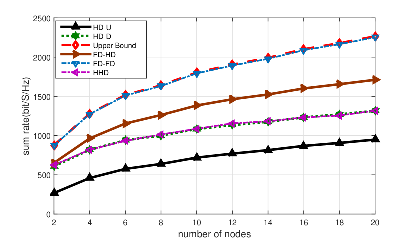
Figure 5: Performance comparison of six schemes in FD and HD networks in the outdoor scenario.

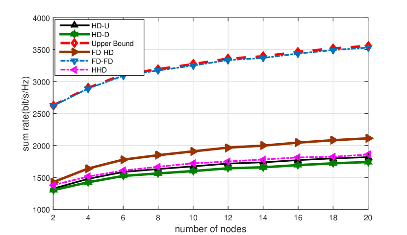
Figure 6: Performance comparison of six schemes in FD and HD networks in the indoor scenario.

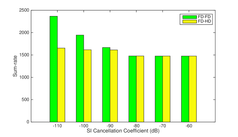
Figure 7: Effect of the self interference cancellation coefficient on the FD network capacity in the indoor scenario.

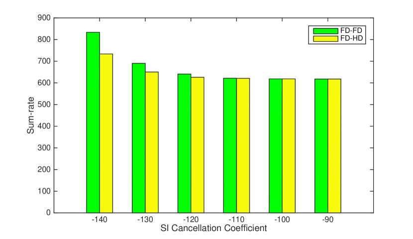
Figure 8: Effect of the self interference cancellation coefficient on the FD network capacity in the outdoor scenario

Fig. 8 compares the sum-rates of an FD-FD network and an FD-HD network for different values of $\beta$ in the indoor scenario. It can be seen that when $\beta$ is larger than a specified threshold, which is near $-90$ dB, there is no difference between the sum-rate of the all HD user case and the sum-rate of the all FD user case. The reason is that when $\beta$ is large relative to the inter-node interference, FD users prefer to work in HD mode in order to increase their rate, hence the sum-rates of FD-FD and FD-HD become equal.

In Fig. 8, the same experiment is repeated for the outdoor scenario. Here the threshold $\beta$ is approximately $-120$ dB which is much smaller than in the indoor case. Since the inter-node interference in the outdoor environment is smaller, the SI cancellation coefficient should be very small to make the FD mode worthwhile for the FD users.

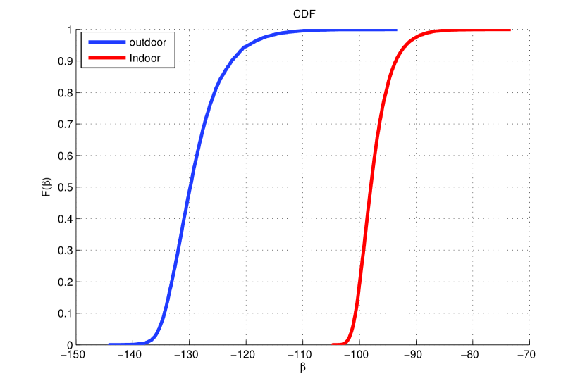
Figure 9: Cumulative Distribution Function of the threshold $\beta$ for the indoor and outdoor environment

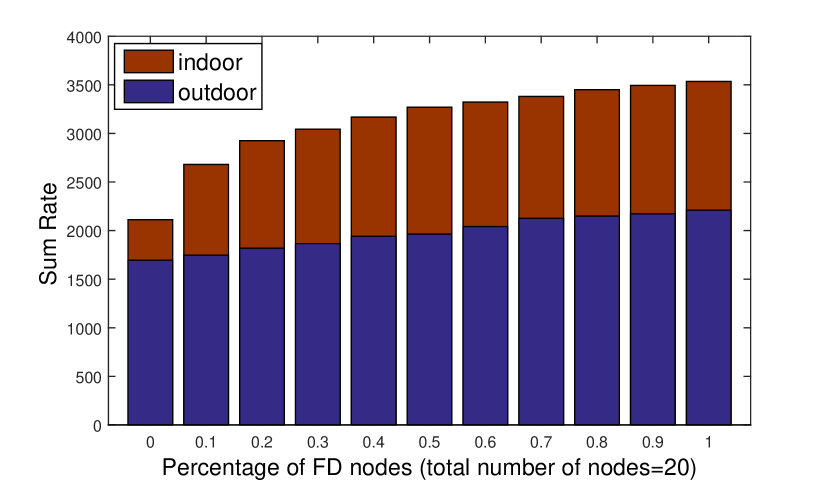
Figure 10: Effect of the fraction of FD nodes on the network throughput in both indoor and outdoor scenarios

Fig. 10 shows the CDF of the threshold $\beta$ for both indoor and outdoor environments based on the analysis in Proposition 2. As evident, in the indoor and outdoor scenarios, the CDF curve almost reaches one for a threshold $\beta$ close to $-90$ dB and $-120$ dB, respectively. These results match those in Fig. 8 and Fig. 8 obtained through simulations. Therefore, the presented analysis is able to accurately predict the required self-interference cancellation performance.

Fig. 10 shows the performance of a full-duplex OFDMA network with a mix of FD and HD users. A total of 20 users are considered, assuming perfect SI cancellation for FD devices. It can be seen that increasing the percentage of FD users in an outdoor environment does not increase the total sum-rate significantly, but in the indoor case by equipping only $10\%$ of the nodes with FD technology the network throughput greatly increases. The reason behind this is the large inter-node interference in the indoor environment that could be avoided by using FD users instead of HD ones.

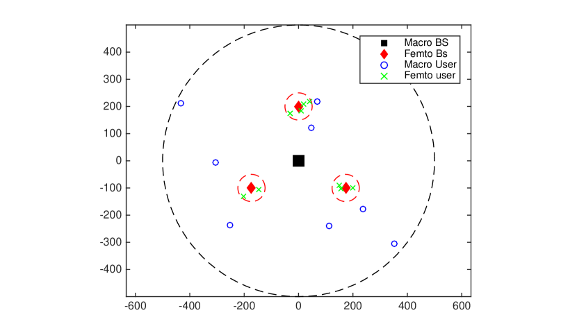
Figure 11: Network topology

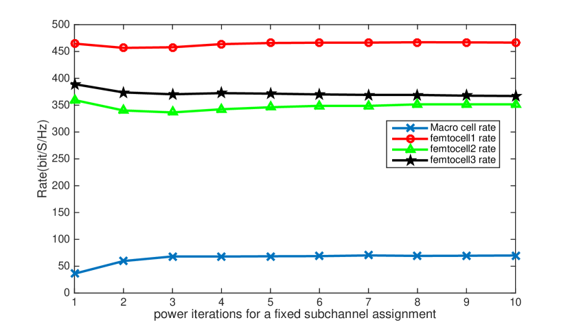
Figure 12: Convergence of the power allocation algorithm

For the heterogeneous OFDMA network, we consider a macro BS with 8 users and 3 femto cell BSs with 2, 3, and 4 users, respectively. The location of base stations and users are depicted in Fig. 12. We assumed that macro users and femto users are randomly spread within a cell radius of 500 m and 50 m around their related BSs, respectively.

Fig. 12 shows the convergence of the power allocation algorithm of Section IV for a fixed sub-channel assignment in the said heterogeneous network. Here, the minimum downlink and uplink rates for macro cell users are set to $R_{mind}=35$ bit/s/Hz and $R_{minu}=35$ bit/s/Hz, respectively. The total rate of macro users is then to be larger than $70$ bit/s/Hz. As we see in this figure, this constraint is satisfied after a few iterations. Also it was expected that this inequality constraint should be satisfied with equality, since if the total rate of macro users becomes bigger than the constraint it increases extra interference for femto cells and reduce the objective function.

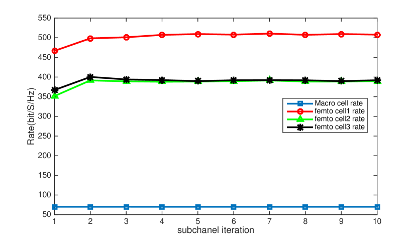
Figure 13: Convergence of the iterative subchannel allocation algorithm

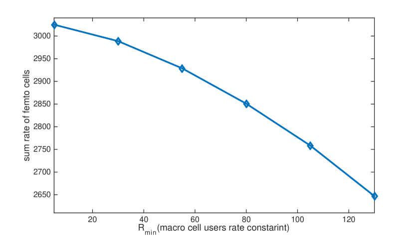
Figure 14: Tradeoff between femto cell throughput and macrocell $R_{min}$

Fig. 14 shows the convergence of the iterative sub-channel allocation algorithm. It can be seen that the femto cell rates converge after a few iterations, while the minimum rate for macro cell users is satisfied.

Fig. 14 depicts the sum-rate of femto cells as a function of the minimum required rate for the macro cell. As evident, the larger the macro cell rate, the smaller the femto cells sum-rate. The reason is that by increasing the rate of the macro cell, the interference caused by macro cell to the femto cell would also increase, thereby reducing the femto cells sum-rate.

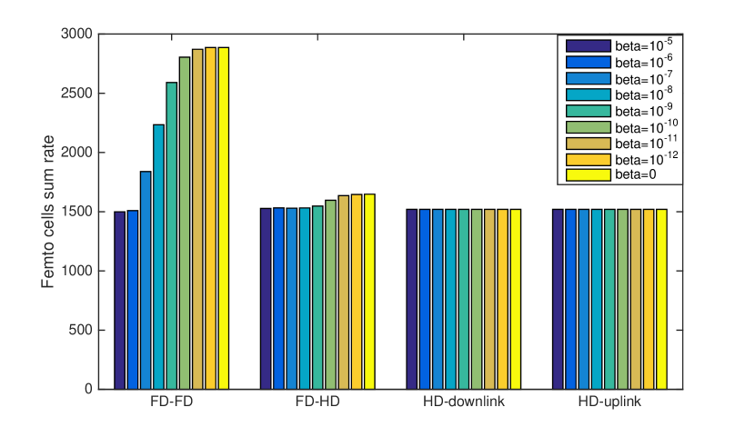
Figure 15: femto cells sum rate for four different schemes and different $\beta$s

Fig. 15 shows the femto cells sum-rate for different schemes (FD-FD, FD-HD, HD-downlink, HD-uplink) and different self interference cancellation coefficient values. The $\beta$ threshold effect is also obvious in this graph and its value is different from the previous sections because of the adopted path loss model and different distances in the heterogeneous setting. In this case, one cannot double the capacity by FD transmission because of the interference generated by other femto cells. Still, significant gains maybe achieved if users adopt the FD technology.

VIII conclusion

In order to fully exploit the advantages of FD technology in wireless networks, it is important to design appropriate resource allocation algorithms that consider the FD capability of the nodes and the BSs. In this paper, first we considered a single cell OFDMA network that contains an FD BS and a mixture of HD and FD users, and also assumed that FD nodes are not necessarily perfect FD devices and may suffer from residual self-interference. For this model, we proposed a sub-channel allocation algorithm and power allocation method and showed that when all users and the BS have perfect FD transceivers, we can double the capacity. Otherwise, because of inter-node interference and self-interference the spectral efficiency gain is smaller, but we showed that even by using an imperfect FD BS in a network, the network throughput could increase significantly. Then, we used the extended version of the proposed algorithms to solve an optimization problem for an FD OFDMA heterogeneous network in which inter-cell interference should be taken into account. We also investigated FD operation in both outdoor and indoor scenarios and studied the effect of the self interference cancellation coefficient and of the percentage of FD users. Finally, we analyzed the effect of the SI cancellation level on the network performance and numerically computed the CDF of the SI cancellation coefficient threshold which had been observed in the simulation results.

References

- [1] D. Korpi, L. Anttila, V. Syrjala, and M. Valkama, “Widely linear digital self-interference cancellation in direct-conversion full-duplex transceiver,” IEEE Journal on Selected Areas in Communications, vol. 32, no. 9, pp. 1674–1687, 2014.
- [2] B. Kaufman, J. Lilleberg, and B. Aazhang, “Analog baseband cancellation for full-duplex: An experiment driven analysis,” arXiv preprint arXiv:1312.0522, 2013.
- [3] E. Ahmed and A. M. Eltawil, “All-digital self-interference cancellation technique for full-duplex systems,” IEEE Transactions on Wireless Communications, vol. 14, no. 7, pp. 3519–3532, 2015.
- [4] M. Duarte, C. Dick, and A. Sabharwal, “Experiment-driven characterization of full-duplex wireless systems,” IEEE Transactions on Wireless Communications, vol. 11, no. 12, pp. 4296–4307, 2012.
- [5] D. Bharadia, E. McMilin, and S. Katti, “Full duplex radios,” in Proceedings of the ACM SIGCOMM, 2013.
- [6] S. Goyal, P. Liu, S. Hua, and S. Panwar, “Analyzing a full-duplex cellular system,” in Proc. Conference on Information Sciences and Systems (CISS), 2013.
- [7] R. Sultan, L. Song, K. G. Seddik, Y. Li, and Z. Han, “Mode selection, user pairing, subcarrier allocation and power control in full-duplex OFDMA hetnets,” in IEEE International Conference on Communication Workshop, 2015.
- [8] B. Di, S. Bayat, L. Song, and Y. Li, “Radio resource allocation for full-duplex OFDMA networks using matching theory,” in IEEE Conference on Computer Communications Workshops (INFOCOM WKSHPS), 2014.
- [9] C. Nam, C. Joo, and S. Bahk, “Joint subcarrier assignment and power allocation in full-duplex OFDMA networks,” IEEE Transactions on Wireless Communications, vol. 14, no. 6, pp. 3108–3119, June 2015.
- [10] ——, “Radio resource allocation with inter-node interference in full-duplex OFDMA networks,” in IEEE International Conference on Communications (ICC), 2015.
- [11] H. Malik, M. Ghoraishi, and R. Tafazolli, “Suboptimal radio resource management for full-duplex enabled small cells,” in IEEE International Conference on Communications Workshops (ICC Workshops), 2017.
- [12] I. Randrianantenaina, H. Dahrouj, H. Elsawy, and M.-S. Alouini, “Interference management in full-duplex cellular networks with partial spectrum overlap,” IEEE Access, vol. 5, pp. 7567–7583, 2017.
- [13] S. Sekander, H. Tabassum, and E. Hossain, “Decoupled uplink-downlink user association in multi-tier full-duplex cellular networks: A two-sided matching game,” IEEE Transactions on Mobile Computing, vol. 16, pp. 2778–2791, 2016.
- [14] P. Aquilina, A. C. Cirik, and T. Ratnarajah, “Weighted sum rate maximization in full-duplex multi-user multi-cell mimo networks,” IEEE Transactions on Communications, vol. 65, no. 4, pp. 1590–1608, 2017.
- [15] I. Atzeni, M. Kountouris, and G. C. Alexandropoulos, “Performance evaluation of user scheduling for full-duplex small cells in ultra-dense networks,” in Proceedings of 22th European Wireless Conference. VDE, 2016, pp. 1–6.
- [16] J.-H. Yun, “Intra and inter-cell resource management in full-duplex heterogeneous cellular networks,” IEEE Transactions on Mobile Computing, vol. 15, no. 2, pp. 392–405, 2016.
- [17] H. Tuy, Convex analysis and global optimization. Springer Science & Business Media, 2013, vol. 22.
- [18] H. H. Kha, H. D. Tuan, and H. H. Nguyen, “Fast global optimal power allocation in wireless networks by local DC programming,” IEEE Transactions on Wireless Communications, vol. 11, no. 2, pp. 510–515, February 2012.
- [19] M. R. Mili, P. Tehrani, and M. Bennis, “Energy-efficient power allocation in OFDMA D2D communication by multiobjective optimization,” IEEE Wireless Communications Letters, vol. 5, no. 6, pp. 668–671, 2016.
- [20] P. Tehrani, F. Lahouti, and M. Zorzi, “Resource allocation in OFDMA networks with half-duplex and imperfect full-duplex users,” in IEEE International Conference on Communications (ICC), 2016.
- [21] K. Seong, M. Mohseni, and J. M. Cioffi, “Optimal resource allocation for OFDMA downlink systems,” in IEEE International Symposium on Information Theory, 2006.
- [22] J. Huang, V. G. Subramanian, R. Agrawal, and R. Berry, “Joint scheduling and resource allocation in uplink OFDM systems for broadband wireless access networks,” IEEE Journal on Selected Areas in Communications, vol. 27, no. 2, pp. 226–234, February 2009.