Abstract

Recording atomic-resolution transmission electron microscopy (TEM) images is becoming increasingly routine. A new bottleneck is then analyzing this information, which often involves time-consuming manual structural identification. We have developed a deep learning-based algorithm for recognition of the local structure in TEM images, which is stable to microscope parameters and noise. The neural network is trained entirely from simulation but is capable of making reliable predictions on experimental images. We apply the method to single sheets of defected graphene, and to metallic nanoparticles on an oxide support.

1 Introduction

With the developments in transmission electron microscopes that has occurred over the last decade, it has become increasingly common to record and store large amounts of TEM data, often in the form of image sequences. This development has been accelerated by the advent of faster and more sensitive detectors such as the direct detection camera ¹; but also by the development of the Environmental TEM, where it becomes possible to study how e.g. nanoparticles respond to reaction gases in real time.²

As the amount of TEM data available increases, it becomes important to have efficient and automated analysis tools. In many applications, accurate identification and classification of local structure is a crucial first step in deriving useful information from atomic-resolution images. Examples include characterizing the distribution of dopants ³ and defects ⁴, in situ imaging of phase transformations ⁵, structural reordering during materials growth ^{6, 7}, dynamic surface phenomena ⁸ and identification of chemical phases in nanoparticles ⁹.

Analysis methods such as Geometric Phase Analysis (GPA) ¹⁰ are based on the local symmetry and periodicity, and has been very successful at extracting structural information in many regular structures, including identifying defects, strain and phase boundaries.¹¹. However, GPA typically has difficulties analyzing e.g. surfaces, where the periodicity changes rapidly.¹²

Real space approaches typically either rely on direct identification of atomic positions by finding local intensity extrema,^{13, 14} or on direct comparison with a template¹⁵. However, these methods are in general not able to compete with a trained human expert. The difficulties arise in part due to the phase contrast nature of high resolution TEM, which makes the image extremely sensitive to small changes in the defocus, necessitating human intervention in the image analysis. When analyzing image sequences, it may even be necessary to adjust the image analysis tools to each frame, as small rotations, vibrations and thermal drift can modify the appearance from one frame to another. These difficulties are compounded by the low signal-to-noise ratio resulting from using the smallest possible electron dose to minimize beam damage to the sample.

Recently, convolutional neural networks and related deep-learning methods have demonstrated excellent performance in visual recognition tasks, including particle detection¹⁶ and automatic segmentation of brain images from cryo-electron microscopy images.¹⁷ Kirschner and Hillebrand have published a method for predicting defocus and sample thickness¹⁸, and Meyer and Heindl have used neural networks to reconstruct the exit wave function from off-axis electron holograms¹⁹.

Whereas deep learning methods have recently been proposed to analyse Scanning TEM (STEM) images²⁰, but have to our knowledge not yet been used to analyze the atomic structure in high resolution HRTEM images. In this article, we describe a CNN based method for classifying atomic structures in TEM, and demonstrate that it can be applied to single layers of graphene, as well as to supported metallic nanoparticles. Under good circumstances, the method can be generalized to identify chemical species and to identify the height of atomic columns.

2 Methods

The task of identifying atoms in atomically resolved TEM images is a special case of a general problem in image analysis. The task is to identify instances of a set of structures, and assigning class labels $\{c_{n}\}$ and Cartesian coordinates $\{(x_{n},y_{n})\}$ to each of them. In the simplest case, there is only one class (“atom”), but the analysis can be extended to identify specific structures of atoms; atom columns of various sizes; vacancies; etc. The neural network will be looking for a predefined set of $N_{c}$ labels, $C=\{c_{0},c_{1},\ldots,c_{N_{c}}\}$ and will initially assign a probability for each possible label. The choice of how to categorize the structures is problem specific, and typically depends on how the researcher derives meaning from the image.

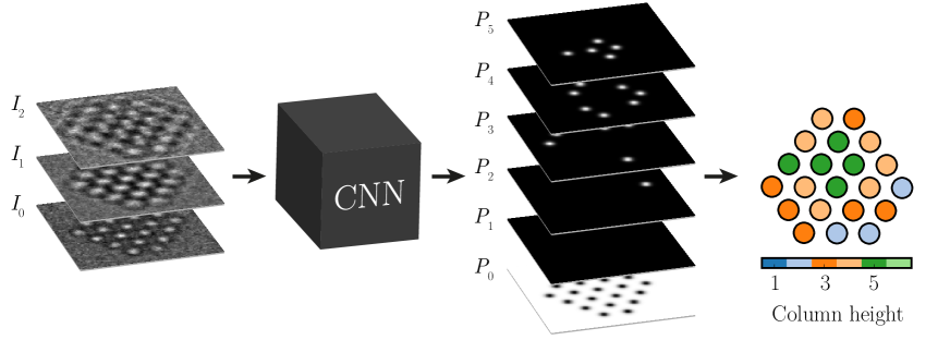
Figure 1: The classification method illustrated on a focal series of three images of a gold nanoparticle. The convolutional neural net is fed one or more TEM images of the same sample with varying microscope parameters. The task of the CNN is to classify each pixel as belonging to one of six categories: background or an atomic column 1–5 atoms high. The output of the CNN is thus six probability maps, which are converted into an interpretation of the structure.

An example is shown in Fig. 1, where one or more images of a structure is mapped onto a set of probability maps, from which the interpreted structure can be depicted. The input will typically be a single grey-scale image of size $N_{x}\times N_{y}$, but it is possible to use multiple images of the same spatial region, for example a focal series where the microscope focus is varied systematically. Thus in general the neural network maps image data $I_{x,y,k}$ of shape $N_{x}\times N_{y}\times N_{f}$ (where $N_{f}$ is often $1$) to probability maps $P_{x,y,k}$ of shape $N_{x}\times N_{y}\times N_{c}$, where $N_{c}$ is the number of classes including a background class. Including the background class makes it easy to enforce normalization of the probabilities,

$$\forall x,y:\qquad\sum_{k}P_{x,y,k}=1.$$ (1)

With such a classification scheme, it is important that structures do not overlap, and overlapping structures should be handled by defining new classes. An example is columns of atoms, which can be handled by making classes for a single atom, a column of two atoms, etc.

2.1 Preprocessing

Contrast and illumination may vary significantly across experimentally obtained TEM images, in particular if images contain local structures that are not relevant for the problem being analyzed. This is handled by a combination of subtractive and divisive normalization. First, a local average of the intensity is subtracted from the image

$$G_{ijk}=I_{ijk}-\frac{1}{N_{f}}\sum_{pqk^{\prime}}w_{pq}I_{i+p,j+q,k^{\prime}}$$ (2)

where $w_{pq}$ is a Gaussian weighting window normalized so $\sum_{pq}w_{pq}=1$. The decay length of the Gaussian weighting window must be chosen to be significantly longer than the length scales of the features the net should detect, to avoid washing them out.

Finally, the contrast is normalized with a divisive normalization using the same Gaussian weighting window

$$H_{ijk}=\frac{G_{ijk}}{\frac{1}{N_{f}}\sqrt{\sum_{pqk^{\prime}}w_{pq}G^{2}_{i+p,j+q,k^{\prime}}}}$$ (3)

2.2 Neural net architecture

The neural network needs to be able to combine information on multiple length scales. Locally, the atoms are identified as local peaks or valleys, but estimating what an atom should look like requires contextual information since it depends on e.g. the defocus of the microscope. In some images the atoms may be bright spots, in other they are dark spots, and the contrast may even invert within different regions of the same image.

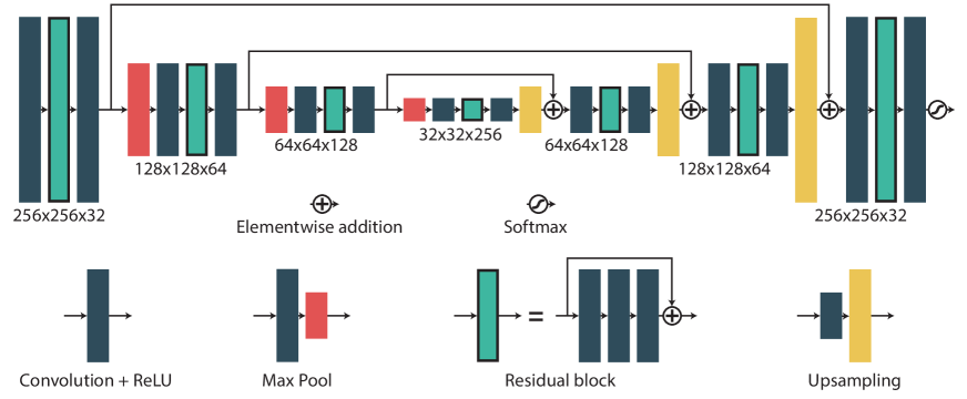
Figure 2: The architecture of the neural network. Information flows from left to right. The features are down-sampled in an encoding path and up-sampled through a decoding path, in addition several skip connections ensure that it is possible to retain fine spatial information.

The network architecture is based on fully convolutional networks (FCN) for pixel-wise segmentation²¹. Following the FusionNet structure proposed by Quan et al. ¹⁷ we use additive skips and residual blocks to prevent vanishing gradients and to allow for training of deeper neural nets. Multi-level up-sampling and skip connections combine global abstract information from deep coarse paths with local spatially resolved information from shallow paths.

The network has a single pipeline with additive skip connections to preserve spatial information at each resolution. The lowest resolution is one eighths of the full resolution, this allows for spatial filters to be applied that compare features across the entire image. The shape of the network is chosen to be symmetric, so for every layer present in the part where resolution is reduced, there is a corresponding layer in the part where resolution is increased again. The chosen architecture is shown in Fig. 2

At each resolution on the down-sampling and up-sampling paths, the network consists of five convolutional layers, with a skip connection bypassing the middle three layers using elementwise addition (shown as a residual block in Fig. 2). Every convolutional layer except the last employ a $3\times 3$ convolutional kernel, followed by an element-wise rectified linear activation, $h(x)=\max\{0,x\}$, which are then batch normalized following eq. (2–3) ²².

Feature compression is done in the down-sampling path using a max pooling layer down-sampling by a factor two in both spatial direction, while doubling the number of feature maps. Conversely, in the up-sampling path the features are up-sampled using a transpose convolutional block²¹ doubling the spatial resolution while halving the number of feature maps, followed by an element-wise addition from same level of the encoding path, forming a long skip connection.

The final scoring consists of a convolutional layer with a $1\times 1$ kernel followed by a softmax non-linearity

$$\sigma(P_{k})=\frac{\exp(P_{k})}{\sum_{k=1}^{m_{f}}\exp(P_{k})}\,.$$ (4)

The transpose convolutional layers are initialized as bilinear interpolation and all other layers use random weight initialization.

The network is implemented with TensorFlow using the Python API,²³ chosen due to the wide range of functions already made available, as well as the community support. All models are trained and tested with TensorFlow on a single NVIDIA GTX 1080 Ti. Our models and code are publicly available.²⁴

2.3 Generation of training data

A particular challenge is to generate the training data for the neural net, since on one hand these data should include the kind of structures the net should be able to recognize, but on the other hand should not bias the network towards a specific interpretation of the images. This makes it particularly difficult to use real experimental data as training data, since the network would be trained to reproduce any subconscious bias of the scientists generating the interpretations to which the net is trained.

Instead, we train the network to a large set of simulated data. It is important to be aware that this does not preclude biasing the training set, since such a bias will always be present in the selection criteria generating the structures that form the basis for the image simulations, but at least the true positions of all atoms are known for the simulated images.

We try to minimize the bias of the models by generating a training set with a rather large random component while still maintaining realistic atomic positions, but without resorting to e.g. thermodynamical modelling of the systems; this will be discussed further in the sections describing applications of the method.

The training set consists of a collection of computer generated systems (e.g. nanoparticles, if the neural net is to be applied to such), generated using the Atomic Simulation Environment (ASE) ²⁵. Simulated images are generated using the Multislice Algorithm,²⁶. Simulation is done using the publicly available QSTEM code²⁷, through a Python interface to ASE developed by the authors ¹². The exit wave functions for each system in the training set is precomputed, but during training simple symmetry operations (translation, rotation by 90^∘ and mirroring) can easily be applied in each training step.

parameters	lower bound	upper bound	distribution
defocus ($\Delta f$)	-200 Å	200 Å	uniform
3rd order spherical ($C_{s}$)	-20 $\mu$m	20 $\mu$m	uniform
5th order spherical ($C_{5}$)	0	5 mm	uniform
1st order astigmatism magnitude	0	100 Å	uniform
1st order astigmatism angle	0	2$\pi$	uniform
deflection	0	25 Å	uniform
focal spread	20 Å	40 Å	uniform
dose	$10^{1}$ $e^{-}/\text{\AA}^{2}$	$10^{4}$ $e^{-}/\text{\AA}^{2}$	exponential
$c_{1}$ (MTF)	0	0.1	uniform
$c_{2}$ (MTF)	0.4	0.6	uniform
$c_{3}$ (MTF)	2	3	uniform

Table 1: Randomized parameters for generating training examples of graphene for a 80 kV microscope.

For each training iteration, a Contrast Transfer Function (CTF) is generated with randomly chosen parameters for the electron microscope taken from a distribution; Table 1 shows an example of parameters used for graphene. The CTF is then applied to the precomputed exit wave function. The effect of energy spread (i.e. temporal coherence) is included in the quasi-coherent approximation²⁹, and temperature effects are included by blurring the atomic potentials. The images are resampled to a random sampling rate, a technique sometimes referred to as scale-jittering. It is essential to include a reasonable model of noise in the images, this is done by modelling the finite electron dose with a Poisson distribution, and including the modulation transfer function (MTF) of the detector in the image simulation. The latter is essential as it has a strong influence on the spectral properties of the noise, and prevents that the network is trained incorrectly to detect atoms by the absence of pure white noise. The MTF is modelled as ²⁸:

$$\mathrm{MTF}(q)=\frac{1-c_{1}}{1+\left(\frac{q}{2c_{2}q_{N}}\right)^{c_{3}}}+c_{1}\quad,$$ (5)

where $q_{N}$ is the Nyquist frequency.

The ground truth for the training data is generated as a superposition of Gaussians with an amplitude of one, centered at the positions of the atoms (or the mean of the positions for atomic columns). The background class is then assigning the remaining probability, such that the sum of probabilities is one; this is possible since the overlap between any pair of Gaussians is negligible. The width, $\sigma$, of the Gaussians is an important parameter, since it strongly influences the penalty of wrongly assigning a region of the inferred confidence map to the background. We found that a too small value of $\sigma$ would lead to a network with a strong tendency to assign any region that is difficult to analyze (e.g. due to noise) to the background class. In a similar way, we found that a common local minimum at training would be to assign anything to the background class, this is also exacerbated by a low value of $\sigma$. We found that a width of $\sigma=1$Å, corresponding to 8–10 pixels at typical resolutions, worked well for the cases we have considered.

2.4 Training

The CNN is trained using a mean squared difference loss function, regularized with a penalty on the size of the $l_{2}$ norm of the weights

$$L=\sum_{ijk}\|\tilde{P}_{ijk}-P_{ijk}\|^{2}+\frac{1}{2}\lambda\sum_{i}W_{i}^{2}$$ (6)

where $\tilde{P}$ is the output and $P$ is the ground truth. The network is mainly regularized through the large variability of the training image data, since a new training image is simulated for every training iteration. Nevertheless, we found that performance on actual experimental data is improved by adding moderate $l_{2}$ regularization (also known as weight decay), since this causes any weight not being used by the network to produce meaningful output to become negligible rather than to persist for no reason. Such weights may deteriorate performance on actual experimental data although they do not negatively impact the performance on the training data.

2.5 Post-processing and interpretation

While the interpretation of the confidence maps is simplest if there is only a single class, we here illustrate how it can be done even in the case of multiple classes.

The first step is identifying the regions where a signal is present. This is done by finding all minima in the confidence map for the background class. Only minima below $\varepsilon=0.995$ on a scale from 0 – 1 are included, this prevents spending time on analyzing regions that are clearly background. The local minima are then used as seeds for basins created using the watershed principle for image segmentation using Meyer’s algorithm ³⁰. We avoid including long tails in segments by setting a hard upper limit for each segment at $\varepsilon$.

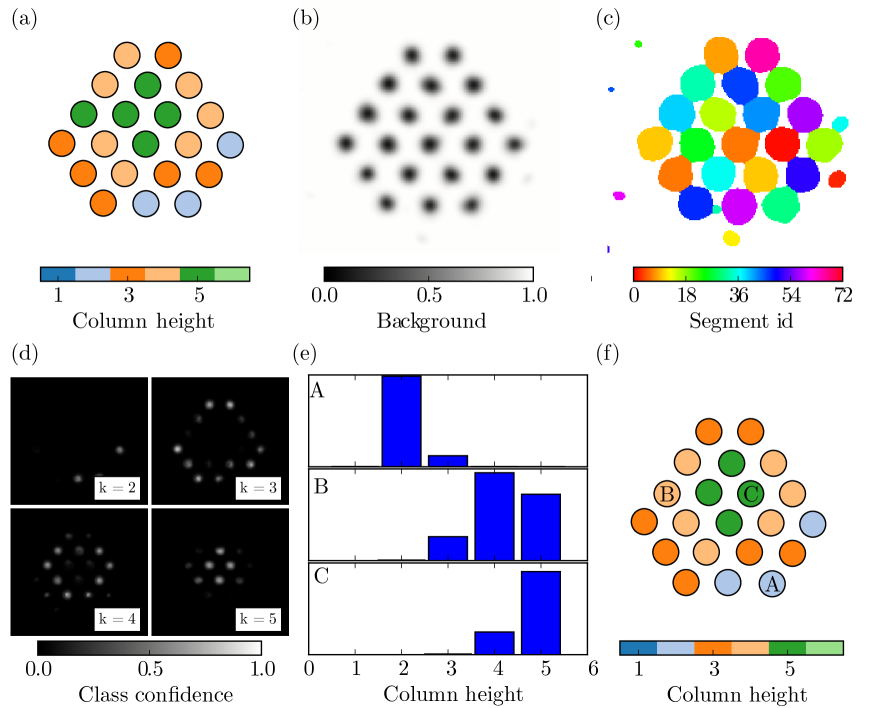
Figure 3: (a) The input to the network is three images of a small nanoparticle, recorded (or simulated) with different defocus; here is shown a single simulated image with the ground truth thickness of the individual columns marked with colors. (b) The background confidence map; we see that the network correctly identifies that there is something at each atomic column, but also thinks there may be something outside the nanoparticle. (c) A segmentation of the background map into several distinct objects. (d) Confidence maps for the classes corresponding to columns containing two to five atoms. (e) Each object is assigned a probability of belonging to each of the five classes. (f) The final classification of the atomic columns. The labels A–C mark the three columns examined in panel (e). In this case, most atomic columns are correctly assigned to their classes. Column B which has five atoms is incorrectly identified as having only four atoms; however the network is clearly in doubt as seen in the probability distribution. One other column is misassigned, in both cases the network has probably learned that columns at edges and corners are likely to contain fewer atoms, which is not the case for these two columns.

Each segment is then assigned a probability for belonging to each non-background class as

$$p_{n}(c_{k})\propto\sum_{i,j\in\mathcal{S}_{n}}P_{ijk}\quad k>0\quad,$$ (7)

where the sum is over all pixels belonging to the $n$’th image segment. The coordinate of the atomic structure is calculated as the center-of-mass of the image segment. Finally, segments are discarded if

$$\sum_{k>0}p_{n}(c_{k})<tp_{n}(c_{0})$$ (8)

The value chosen for $t$ is normally uncritical, but values near 0.5 are recommended. It should be noted that in most cases there is only a single class ($c_{1}$), “an atom”. The process is illustrated in Fig. 3.

3 Application to graphene

High resolution TEM has been used extensively to study graphene, and several automatic algorithms for extracting quantitative information have been proposed ^{31, 32, 33}. Of particular interest is the ability to identify defects, both localized (vacancies, dislocations etc) and extended (grain boundaries).

3.1 Training

It is an easy task for a CNN to recognize the regular hexagonal lattice of graphene. However, we want the network to be able to correctly localize the atomic positions also in situations where they are not at or near their ideal positions. Thus, the atomic models used to generate the training images cannot simply be ideal sheets of graphene, nor can they be sheets of graphene with added defects.

The opposite extreme, that of generating purely random atomic positions, would result in inefficient networks as the vast majority of the training data would be very different from the experimentally interesting situations. Instead, we generate atomic positions that lie somewhere between these two extremes.

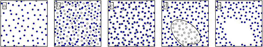
Figure 4: Procedure for generating training structures for graphene. (a) A square in 2D space is filled with randomly distributed seed points under the constraint of a minimum separation in terms of euclidean distance. (b) Next, the Voronoi tessellation is generated from the seed points, the vertices of the diagram will become atomic positions while the original positions are discarded. (c) To avoid overlapping atoms, the positions of the Voronoi vertices are relaxed using Lloyd’s algorithm. (d) Lastly, zero to four holes of varying size and shape are introduced in the structure, resulting in the structure seen in (e).

The algorithm is based on the observation that a Voronoi tessellation of a 2D set of points mainly consists of hexagons, and is illustrated in Fig. 4. First, an area is filled with randomly distributed points under the constraint of a minimal distance between the points, i.e. a Poisson disc distribution. These points form the generating centers of a Voronoi tessellation; the vertices of the tessellation will become the carbon atoms. The tessellation is optimized by a few steps of Lloyd’s algorithm³⁴: the centers of the Voronoi tessellation are moved to the center of mass of their respective Voronoi cell. This makes the Voronoi polyhedra more regular, and in particular it moves closely placed vertices apart, preventing atoms from being placed unrealistically close. Finally, from zero to four holes are cut randomly in the structure.

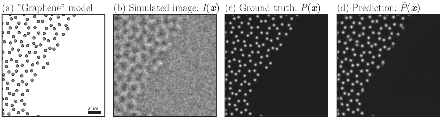
Figure 5: The CNN is trained on simulated images of graphene-like structures, generated by the algorithm in Fig. 4. (a) A quasi-random graphene-like structure. (b) Simulated image based on the atomic positions. (c) The corresponding ground truth calculated from the atomic positions. The network is trained on a series of matching images and ground truth maps. (d) The output prediction of the trained neural network given the simulated image in (b).

The resulting structures form a structure which is very suitable for our purpose. The distribution of bond lengths is quite narrow, and the mean can be controlled by choosing the initial number of points. The structure contains a large number of polygons with five to eight sides, similar to what is observed in graphene grain boundaries. A typical training structure is shown in Fig. 5.

We generated 500 random structures with a size of $43.2\times 43.2$ Å, or $360\times 360$ pixels at a sampling rate of $0.12$ Å/pixel. All the simulations were done at an acceleration voltage of $80$ kV. While the microscope parameters are uniquely generated at each training step, the same structure is utilized multiple times. This have little consequence since most of the variability is in microscope parameters.

3.2 Analyzing experimental images

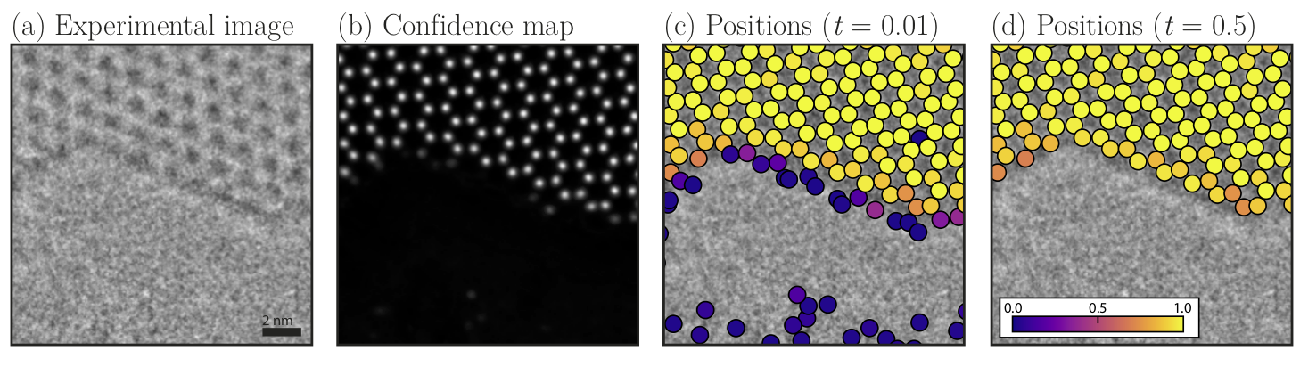
Figure 6: A neural network trained exclusively on simulated data is capable of generalizing to experimental images. (a) Single suspended graphene sheet with a hole formed under the influence of the electron beam. (b) The regressed probability distribution predicted by the neural network for the image in (a). (c) The local peak positions of the probability map is overlayed on the image. The peaks are color-coded according to their maximum value. Peaks with a maximum value less than 0.01 are excluded. (d) A higher tolerance for exclusion is used to remove peaks with a maximum value less than 0.5.

An example of how the network performs on experimental data is given in Fig. 6. When given an experimental TEM image of the edge of a graphene sheet, the neural network has no problems identifying the atoms inside the graphene sheet. At the edge of the sheet, there are positions where the network assigns a small but nonzero probability for the presence of atoms, but using a reasonable cutoff of $t=0.5$ gives a result in agreement with a manual analysis of the image, and without any high-energy atomic configurations at the edges.

We apply the trained neural net on a number of graphene images.^{33, 35} The experimental graphene images were measured using a FEI Titan 80-300 Environmental TEM equipped with a monochromator at the electron gun and spherical aberration ($C_{s}$) corrector on the objective lens. The acceleration voltage of the microscope was 80 kV which is below the knock-on threshold for carbon atoms in pristine graphene.³⁶ The electron beam energy spread was below 0.3 eV, while the $C_{s}$-corrector was aligned to minimize the spherical aberration. The images were recorded using a Gatan US1000 CCD camera with an exposure time of 1 s.

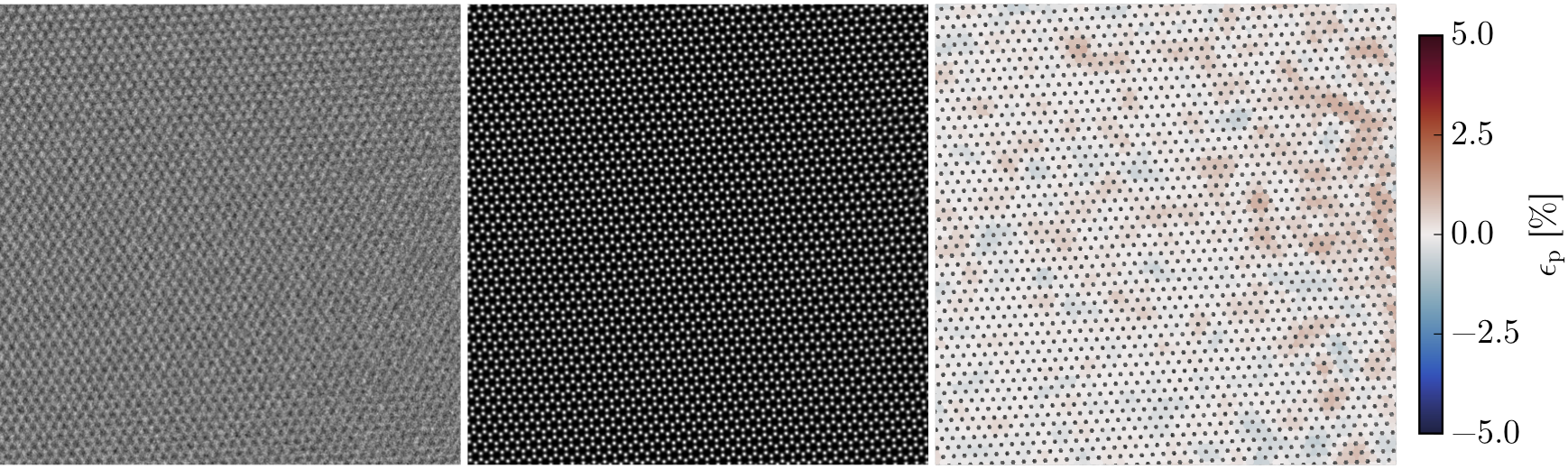
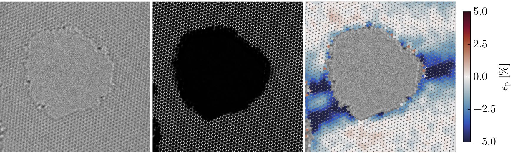
Figure 7: Experimental images of graphene, and their interpretation by the neural net. The first row shows a pristine sheet of graphene, the second a sheet with a hole. The left column shows the original TEM images. The center column shows the output of the neural net. The rightmost column shows the planar strain calculated from the atomic positions, as identified by the neural net.

Fig. 7 shows a TEM images of pristine graphene, and of graphene with a hole. The negative $C_{s}$ imaging results in images where the carbon atoms are bright spots, with the centers of the hexagons appearing dark. The output of the neural network is shown in the central column. The neural network detects all atomic positions in the pristine sheet, this is accomplished without having regular hexagonal lattices in the training set. Additionally, the neural network automatically recognizes that the atoms appear bright, which is only the case for half of the training images. Finally, we show the strain calculated from the atomic positions, using a structural template with the two nearest neighbour shells (i.e. the 9 nearest neighbours), as described previously.¹²

We do not expect any strain in a pristine area of graphene, hence this sample provides a good of the accuracy of the detected positions. We find that the bond lengths are normally distributed around the mean, 1.42 $\mathrm{\AA}$, with a standard deviation of 0.18 $\mathrm{\AA}$. This standard deviation is comparable or smaller to what was found using the method of Vestergaard et al. ³⁵, thus demonstrating, that the positions, determined by our method, are resistant to noise.

4 Application to metallic nanoparticles

Metallic nanoparticles on oxide support is a very active research topic, mainly due to the applications within heterogeneous catalysis. Often, the detailed atomic structure is important for the catalytic process, as the active size depending on the process may be e.g. step sites³⁷, corner atoms³⁸ or strained facets^{39, 40}.

For example, although gold is normally chemically inert, nanoparticles of gold have been shown to catalyse the oxidation of CO to CO₂⁴¹. It is also a system where significant atomic rearrangement is observed in the presence of gas, both involving overall shape changes of the nanoparticles⁴² and changes in the local surface structure We here use supported gold nanoparticles to illustrate the application of neural nets to the analysis of supported nanoparticles.

4.1 Training

We have trained the network on simulated gold nanoparticles. As the network should be able to recognize both atomically flat and rough surfaces, the training set includes both kinds of nanoparticles. Initially, nanoparticles are cut from a regular crystal, keeping a random number of layers in directions with low Miller indices (the $\left<100\right>$, $\left<110\right>$ and $\left<111\right>$ directions). To roughen the particles, a random number of additional atoms are added to the particle. The atoms are added at allowed crystal positions at the surface of the nanoparticles, in such a way that highly coordinated surface sites are most likely to be picked. If the coordination number (i.e. the number of occupied neighbor sites) of site $i$ is $n_{i}$, then the probability of placing the next atom at site $i$ is chosen as

$$p(n_{i})=\frac{\exp\left(n_{i}/T\right)}{\sum_{j}\exp\left(n_{j}/T\right)}$$ (9)

where the sum is over all sites $j$ where $n_{j}\geq 1$ and $T$ is a parameter that can be chosen differently for each nanoparticle to generate particles with different roughness.

Each particle is then aligned into the $\left<110\right>$ or $\left<111\right>$ zone axis, and is rotated a random amount around the zone axis. It is finally tilted 0–5^∘ away from the zone axis.

As was the case for the graphene simulations, 500 nanoparticles were generated, but during the training new microscope parameters were picked for each iteration, and the nanoparticles were randomly translated, mirrored and rotated by a multiple of 90^∘ (operations that can cheaply be performed on the precomputed wave-functions). Figure 8 shows a sample of generated nanoparticles, and their corresponding images.

Figure 8: Top rows: Examples of nanoparticles generated using the algorithm we have proposed. The height of the atomic columns of the nanoparticles are indicated with a color-coding. Middle rows: Simulated images given the atomic models above. Bottom rows: Output from our neural network method given the simulated images. As can be seen, in one of the images the network is not able to identify the atomic columns in the thickest part of the nanoparticle, this is due to a combination of low signal-to-noise ratio in the image, and a significant off-axis tilt smearing out the highest atomic columns.

4.2 Analyzing nanoparticle image sequence

Figure 9: top row: Experimental high resolution TEM image of gold on ceria in an oxygen atmosphere. The pressure was 4.5 Pa and the electron dose per image was $3.1\times 10^{2}$ e^-/Ų (dose rate $1.56\times 10^{3}$ e^-/Ų/s at an exposure time of 0.2 s). Middle row: Output from the neural network given the images above. Bottom row: The atoms identified by the neural net are marked as purple circles overlaid on the original image. The experimental images were measured using a FEI Titan 80-300 Environmental TEM operated at 300 keV.

We applied the resulting network to gold nanoparticles on a ceria substrate. Figure 9 shows a TEM image of such a particle, and the corresponding analysis by the neural net. It is seen that the network confidently identifies the atoms in the nanoparticle, but not in the substrate; this is partly due to the network not being trained on ceria’s crystal structure, partly because the substrate is not in a prominent zone-axis orientation.

In the microscope, a image sequence of this nanoparticle was recorded, Fig. 9 shows four snapshots of this sequence, clearly showing the atomic diffusion processes.

Figure 10: The surface dynamics of gold nanoparticles is influenced by the gaseous atmosphere. The occurence is the percentage of frames where the neural network identified an atomic column at a possible site. And the events are the percentage of frames where a site was previously occupied, but is unoccupied in the frame immediately after, or vice versa.

We used the neural network to analyze TEM image sequences showing surface diffusion on gold nanoparticle in various gasses. Figure 10 shows the same ceria-supported gold nanoparticle in high vacuum and in an oxygen atmosphere. The neural network is applied to each frame in the image sequence, and used to identify the presence (and position) of the atomic columns. Since the network was not trained on substrates, and since atomic resolution may not be obtainable simultaneously in the substrate and the nanoparticle, we only use the network to analyze the metallic nanoparticle and mask out the output of the network corresponding to the substrate.

During the image sequence, atoms at the surfaces and in particular at the corners of the nanoparticle are clearly seen to appear and disappear again, as the surface atoms diffuse on the particle. We illustrate this in the figure in two different ways. In the middle column, atomic columns are colored according to the fraction of time they are present in the image. It is clearly seen that in the presence of oxygen, many of the surface and corner atoms are only present part of the time, indicating surface diffusion. In the rightmost columns, “events” are counted. It is considered an “event” if an atomic column is present in one frame, but absent in the next, or vice versa; this cause the diffusing atoms to light up on the figure. Together, this analysis shows that the presence of oxygen clearly enhances the surface diffusion. This will be the discussed a separate publication.

4.3 Counting atomic columns

We envision that the main application of this technique will be to identify atoms or columns of atoms, as demonstrated in the two afore-mentioned examples. For this kind of applications, it is relatively straight-forward to train a neural net on sets of simulated images, such that the net becomes able to identify the positions of the atoms or atomic columns also in experimentally obtained images.

A far more demanding task is to identify the chemical species of single atoms in 2D materials, or to count the number of atoms in atomic columns in nanoparticles. It does not appear to be possible to train a network that solves this kind of tasks based on a single image. However, using a series of images taken with varying focus settings, it appears to be possible to train such networks to identify multiple mutually exclusive atomic objects, as already hinted in Fig. 3.

The most common method for measuring the height of atomic columns is Scanning Transmission Electron Microscopy (STEM)^{43, 44}. In TEM, the peak intensity is not generally a monotonic function of column heights, and is sensitive to small tilts of the sample. However, Gonnissen et al.⁴⁵ show that in principle the peak profile in TEM contains enough information to reconstruct the height of the atomic column, and that greater accuracy can be obtained with TEM than with STEM, provided that information from all pixels are used and not just the peak intensities. However, no practical demonstration of such a model exist. It has, however, been demonstrated that the number of atoms in a column can be counted by reconstructing the exit wave function from a focal series ⁴⁶.

To address this problem, we have trained a neural net to classify the columns by the number of atoms. The net is trained on focal series of three simulated TEM images. While the absolute defocus cannot be known precisely in practise, it is relatively easy to control the difference in defocus between the images in a focal series. For this reason, we train the network on three images with defocus of $-170\,\text{\AA}+\Delta$, $-40\,\text{\AA}+\Delta$ and $90\,\text{\AA}+\Delta$, where $\Delta$ is a random number in the range $-20\,\text{\AA}$ – $+20\,\text{\AA}$. The sperical aberration was varied between $C_{s}=-10\mu m$ and $C_{s}=-20\mu m$, and all other parameters as reported previously.

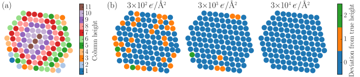
Figure 11: Top row: An example of the input images for the neural net, simulated at three values of the defocus. Bottom row: The performance of the neural net. (a) shows the ground truth, i.e. the actual number of atoms in the atomic columns. (b) shows the error made by the neural network at three different electron doses. The dose given is the sum of the dose in the three images.

An example of the performance is given in Fig. 11. We see that at the highest dose of $3\times 10^{4}e^{-}/\text{\AA}^{2}$, there are no errors. With a dose a 100 times smaller, a significant number of errors appear, but almost all of them are only one-off. It should, however, be noted that this result is obtained under ideal conditions, as the nanoparticle is almost exactly in the $\left<110\right>$ zone axis. When nanoparticles are tilted by up to $3^{\circ}$, the performance is significantly worse, although most errors are still only of a single atom. Figure 12 shows the fraction of errors as a function of electron dose for an ensemble of nanoparticles tilted up to $3^{\circ}$ from the zone axis.

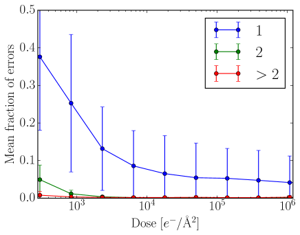
Figure 12: The error rate as a function of electron dose. The three lines show the fraction of atomic columns miscounted by one, two or at least three atoms. The dose is a total for all three images.

We have not verified the viability of the atom counting method on actual experimental TEM images. Doing so would require a significant experimental effort to obtain reliable atomic column heights either from STEM or electron tomography on the same nanoparticles used for the neural net analysis. Such an effort is beyond the scope of this publication, but may be the subject of later reports.

5 Conclusion

We have demonstrated that deep convolutional neural networks can be trained to recognize the local atomic structure in High Resolution Transmission Electron Microscopy images. The network can be trained entirely on simulated data, but is capable of giving interpretations of experimental images that match those of a trained microscopist. We have demonstrated the method both on single layers of defected graphene, and on nanoparticles of gold on a cerium oxide substrate. In addition, we show that neural nets have the potential to determine the height of atomic columns from TEM images.

References

- [1] G. McMullan, A. R. Faruqi, D. Clare, R. Henderson. Ultramicroscopy 2014. 147, 156.
- [2] J. B. Wagner, F. Cavalca, C. D. Damsgaard, L. D. L. Duchstein, T. W. Hansen. Micron 2012. 43, 1169.
- [3] J. C. Meyer, S. Kurasch, H. J. Park, V. Skakalova, D. Künzel, A. Gross, A. Chuvilin, G. Algara-Siller, S. Roth, T. Iwasaki, U. Starke, J. H. Smet, U. Kaiser. Nat. Mater. 2011. 10, 209.
- [4] J. C. Meyer, C. Kisielowski, R. Erni, M. D. Rossell, M. F. Crommie, A. Zettl. Nano Lett. 2008. 8, 3582.
- [5] X. He, T. Xu, X. Xu, Y. Zeng, J. Xu, L. Sun, C. Wang, H. Xing, B. Wu, A. Lu, D. Liu, X. Chen, J. Chu. Sci. Rep. 2014. 4, 6544.
- [6] K. Nagao, T. Inuzuka, K. Nishimoto, K. Edagawa. Phys. Rev. Lett. 2015. 115, 075501.
- [7] X. Li, S. Cheng, S. Deng, X. Wei, J. Zhu, Q. Chen. Sci. Rep. 2017. 7, 40911.
- [8] S. Schneider, A. Surrey, D. Pohl, L. Schultz, B. Rellinghaus. Micron 2014. 63, 52.
- [9] Z. Hussaini, P. A. Lin, B. Natarajan, W. Zhu, R. Sharma. Ultramicroscopy 2017. 186, 139.
- [10] M. J. Hÿtch, E. Snoeck, R. Kilaas. Ultramicroscopy 1998. 74, 131.
- [11] Y. Zhu, C. Ophus, J. Ciston, H. Wang. Acta Mater. 2013. 61, 5646.
- [12] J. Madsen, P. Liu, J. B. Wagner, T. W. Hansen, J. Schiøtz. Adv. Struct. Chem. Imag. 2017. pp. 1–12.
- [13] R. Bierwolf, M. Hohenstein, F. Phillipp, O. Brandt, G. E. Crook, K. Ploog. Ultramicroscopy 1993. 49, 273.
- [14] P. L. Galindo, S. Kret, A. M. Sanchez, J.-Y. Laval, A. Yáñez, J. Pizarro, E. Guerrero, T. Ben, S. I. Molina. Ultramicroscopy 2007. 107, 1186.
- [15] J.-M. Zuo, A. B. Shah, H. Kim, Y. Meng, W. Gao, J.-L. Rouviére. Ultramicroscopy 2014. 136, 50.
- [16] Y. Zhu, Q. Ouyang, Y. Mao. BMC Bioinformatics 2017. 18, 348.
- [17] T. M. Quan, D. G. C. Hildebrand, W.-K. Jeong. arXiv 2016. p. 1612.05360.
- [18] H. Kirschner, R. Hillebrand. Inf. Sci. 2000. 129, 31.
- [19] Meyer, Heindl. J. Microsc. 2008. 191, 52.
- [20] M. Ziatdinov, O. Dyck, A. Maksov, X. Li, X. Sang, K. Xiao, R. R. Unocic, R. Vasudevan, S. Jesse, S. V. Kalinin. ACS nano 2017. 11, 12742.
- [21] E. Shelhamer, J. Long, T. Darrell. IEEE Trans. Pattern Anal. Mach. Intell. 2017. 39, 640.
- [22] S. Ioffe, C. Szegedy. arXiv 2015. p. 1502.03167.
- [23] M. Abadi, P. Barham, J. Chen, Z. Chen, A. Davis, J. Dean, M. Devin, S. Ghemawat, G. Irving, M. Isard, M. Kudlur, J. Levenberg, R. Monga, S. Moore, D. G. Murray, B. Steiner, P. Tucker, V. Vasudevan, P. Warden, M. Wicke, Y. Yu, X. Zheng. In Proceedings of the 12th USENIX Symposium on Operating Systems Design and Implementation (OSDI ’16) 2016 .
- [24] https://github.com/jacobjma.
- [25] A. Hjorth Larsen, J. Jørgen Mortensen, J. Blomqvist, I. E. Castelli, R. Christensen, M. Dułak, J. Friis, M. N. Groves, B. Hammer, C. Hargus, E. D. Hermes, P. C. Jennings, P. Bjerre Jensen, J. Kermode, J. R. Kitchin, E. Leonhard Kolsbjerg, J. Kubal, K. Kaasbjerg, S. Lysgaard, J. Bergmann Maronsson, T. Maxson, T. Olsen, L. Pastewka, A. Peterson, C. Rostgaard, J. Schiøtz, O. Schütt, M. Strange, K. S. Thygesen, T. Vegge, L. Vilhelmsen, M. Walter, Z. Zeng, K. W. Jacobsen. J Phys Condens Matter 2017. 29, 273002.
- [26] P. Goodman, A. F. Moodie. Acta Crystallogr. A 1974. 30, 280.
- [27] C. Koch. Determination of core structure periodicity and point defect density along dislocations. Ph.D. thesis, Arizona State University 2002.
- [28] Z. Lee, H. Rose, O. Lehtinen, J. Biskupek, U. Kaiser. Ultramicroscopy 2014. 145, 3.
- [29] E. J. Kirkland. Advanced Computing in Electron Microscopy. Springer US, 978-1-4419-6532-5, 2 edn. 2010.
- [30] E. R. Dougherty. Mathematical morphology in image processing. M. Dekker, New York 1993.
- [31] C. Kramberger, J. C. Meyer. Ultramicroscopy 2016. 170, 60.
- [32] A. Mittelberger, C. Kramberger, C. Hofer, C. Mangler, J. C. Meyer. Microsc. Microanal. 2017. 23, 809.
- [33] J. S. Vestergaard, J. Kling, A. B. Dahl, T. W. Hansen, J. B. Wagner, R. Larsen. Microsc. Microanal. 2014. 20, 1772.
- [34] S. P. Lloyd. IEEE Trans. Inf. Theory 1982. 28, 129.
- [35] J. Kling, J. S. Vestergaard, A. B. Dahl, N. Stenger, T. J. Booth, P. Bøggild, R. Larsen, J. B. Wagner, T. W. Hansen. Carbon 2014. 74, 363.
- [36] A. Zobelli, A. Gloter, C. P. Ewels, G. Seifert, C. Colliex. Phys. Rev. B 2007. 75, 245402.
- [37] K. Honkala, A. Hellman, I. N. Remediakis, A. Logadottir, A. Carlsson, S. Dahl, C. H. Christensen, J. K. Nørskov. Science 2005. 307, 555.
- [38] S. H. Brodersen, U. Grønbjerg, B. Hvolbæk, J. Schiøtz. J. Catal. 2011. 284, 34.
- [39] I. E. L. Stephens, A. S. Bondarenko, U. Grønbjerg, J. Rossmeisl, I. Chorkendorff. Energy Environ. Sci. 2012. 5, 6744.
- [40] M. Escudero-Escribano, P. Malacrida, M. H. Hansen, U. G. Vej-Hansen, A. Velazquez-Palenzuela, V. Tripkovic, J. Schiøtz, J. Rossmeisl, I. E. L. Stephens, I. Chorkendorff. Science 2016. 352, 73.
- [41] M. Haruta, T. Kobayashi, H. Sano, N. Yamada. Chem. Lett. 1987. 16, 405.
- [42] T. Uchiyama, H. Yoshida, Y. Kuwauchi, S. Ichikawa, S. Shimada, M. Haruta, S. Takeda. Angew. Chem. Int. Ed. Engl. 2011. 50, 10157.
- [43] L. Jones, K. E. MacArthur, V. T. Fauske, A. T. J. van Helvoort, P. D. Nellist. Nano Lett. 2014. 14, 6336.
- [44] A. De Backer, L. Jones, I. Lobato, T. Altantzis, B. Goris, P. D. Nellist, S. Bals, S. Van Aert. Nanoscale 2017. 9, 8791.
- [45] J. Gonnissen, A. De Backer, A. J. den Dekker, J. Sijbers, S. Van Aert. Ultramicroscopy 2017. 174, 112.
- [46] F. R. Chen, C. Kisielowski, D. Van Dyck. Micron 2015. 68, 59.