LTH 1153

KEK-TH-2035

YITP-18-09

6th April 2018

The muon g2𝑔2g-2 and α(MZ2)𝛼superscriptsubscript𝑀𝑍2\alpha(M_{Z}^{2}): a new data-based analysis

Alexander Keshavarzi1, Daisuke Nomura2,3 and Thomas Teubner4

1Department of Mathematical Sciences, University of Liverpool, Liverpool L69 3BX, United Kingdom

Email: a.i.keshavarzi@liverpool.ac.uk 2KEK Theory Center, Tsukuba, Ibaraki 305-0801, Japan

3Yukawa Institute for Theoretical Physics, Kyoto University, Kyoto 606-8502, Japan

Email: dnomura@post.kek.jp 4Department of Mathematical Sciences, University of Liverpool, Liverpool L69 3BX, United Kingdom

Email: thomas.teubner@liverpool.ac.uk

Abstract

This work presents a complete re-evaluation of the hadronic vacuum polarisation contributions to the anomalous magnetic moment of the muon, aμhad,VPsuperscriptsubscript𝑎𝜇hadVPa_{\mu}^{\rm had,\,VP} and the hadronic contributions to the effective QED coupling at the mass of the Z𝑍Z boson, Δαhad(MZ2)Δsubscript𝛼hadsuperscriptsubscript𝑀𝑍2\Delta\alpha_{\rm had}(M_{Z}^{2}), from the combination of e+ehadronssuperscript𝑒superscript𝑒hadronse^{+}e^{-}\rightarrow{\rm hadrons} cross section data. Focus has been placed on the development of a new data combination method, which fully incorporates all correlated statistical and systematic uncertainties in a bias free approach. All available e+ehadronssuperscript𝑒superscript𝑒hadronse^{+}e^{-}\rightarrow{\rm hadrons} cross section data have been analysed and included, where the new data compilation has yielded the full hadronic R𝑅R-ratio and its covariance matrix in the energy range mπs11.2subscript𝑚𝜋𝑠11.2m_{\pi}\leq\sqrt{s}\leq 11.2 GeV. Using these combined data and perturbative QCD above that range results in estimates of the hadronic vacuum polarisation contributions to g2𝑔2g-2 of the muon of aμhad,LOVP=(693.26±2.46)×1010superscriptsubscript𝑎𝜇hadLOVPplus-or-minus693.262.46superscript1010a_{\mu}^{\rm had,\,LO\,VP}=(693.26\pm 2.46)\times 10^{-10} and aμhad,NLOVP=(9.82±0.04)×1010superscriptsubscript𝑎𝜇hadNLOVPplus-or-minus9.820.04superscript1010a_{\mu}^{\rm had,\,NLO\,VP}=(-9.82\pm 0.04)\times 10^{-10}. The new estimate for the Standard Model prediction is found to be aμSM=(11 659 182.04±3.56)×1010superscriptsubscript𝑎𝜇SMplus-or-minus11659182.043.56superscript1010a_{\mu}^{\rm SM}=(11\ 659\ 182.04\pm 3.56)\times 10^{-10}, which is 3.7σ3.7𝜎3.7\sigma below the current experimental measurement. The prediction for the five-flavour hadronic contribution to the QED coupling at the Z𝑍Z boson mass is Δαhad(5)(MZ2)=(276.11±1.11)×104Δsuperscriptsubscript𝛼had5superscriptsubscript𝑀𝑍2plus-or-minus276.111.11superscript104\Delta\alpha_{\rm had}^{(5)}(M_{Z}^{2})=(276.11\pm 1.11)\times 10^{-4}, resulting in α1(MZ2)=128.946±0.015superscript𝛼1superscriptsubscript𝑀𝑍2plus-or-minus128.9460.015\alpha^{-1}(M_{Z}^{2})=128.946\pm 0.015. Detailed comparisons with results from similar related works are given.

1 Introduction

The anomalous magnetic moment of the muon, aμ=(g2)μ/2subscript𝑎𝜇subscript𝑔2𝜇2a_{\mu}=(g-2)_{\mu}/2, stands as an enduring test of the Standard Model (SM), where the 3.5σsimilar-toabsent3.5𝜎\sim 3.5\sigma (or higher) discrepancy between the experimental measurement aμexpsuperscriptsubscript𝑎𝜇expa_{\mu}^{\rm exp} and the SM prediction aμSMsuperscriptsubscript𝑎𝜇SMa_{\mu}^{\rm SM} could be an indication of the existence of new physics beyond the SM. For aμexpsuperscriptsubscript𝑎𝜇expa_{\mu}^{\rm exp}, the value is dominated by the measurements made at the Brookhaven National Laboratory (BNL) [1, 2, 3], resulting in a world average of [4]

aμexp=11 659 209.1(5.4)(3.3)×1010.superscriptsubscript𝑎𝜇exp11659209.15.43.3superscript1010a_{\mu}^{\rm exp}=11\ 659\ 209.1\ (5.4)\ (3.3)\times 10^{-10}\,. (1.1)

Efforts to improve the experimental estimate at Fermilab (FNAL) [5] and at J-PARC [6] aim to reduce the experimental uncertainty by a factor of four compared to the BNL measurement. It is therefore imperative that the SM prediction is also improved to determine whether the g2𝑔2g-2 discrepancy is well established.

The uncertainty of aμSMsuperscriptsubscript𝑎𝜇SMa_{\mu}^{\rm SM} is completely dominated by the hadronic contributions, aμhadsuperscriptsubscript𝑎𝜇hada_{\mu}^{\rm had}, attributed to the contributions from the non-perturbative, low energy region of hadronic resonances. The hadronic contributions are divided into the hadronic vacuum polarisation (VP) and hadronic light-by-light (LbL) contributions, which are summed to give

aμhad=aμhad,VP+aμhad,LbL.superscriptsubscript𝑎𝜇hadsuperscriptsubscript𝑎𝜇hadVPsuperscriptsubscript𝑎𝜇hadLbLa_{\mu}^{\rm had}=a_{\mu}^{\rm had,\,VP}+a_{\mu}^{\rm had,\,LbL}\,. (1.2)

This analysis, KNT18, is a complete re-evaluation, in line with previous works [7, 8, 9], of the hadronic vacuum polarisation contributions, aμhad,VPsuperscriptsubscript𝑎𝜇hadVPa_{\mu}^{\rm had,\,VP}. The hadronic vacuum polarisation contributions can be separated into the leading-order (LO) and higher-order contributions, where the LO and next-to-leading order (NLO) contributions are calculated in this work.111The next-to-next-to-leading order (NNLO) contributions have recently been determined in [13] and are included as part of aμSMsuperscriptsubscript𝑎𝜇SMa_{\mu}^{\rm SM} below. These are calculated utilising dispersion integrals and the experimentally measured cross section,

σhad,γ0(s)σ0(e+eγhadrons+γ)subscriptsuperscript𝜎0had𝛾𝑠superscript𝜎0superscript𝑒superscript𝑒superscript𝛾hadrons𝛾\sigma^{0}_{{\rm had},\gamma}(s)\equiv\sigma^{0}(e^{+}e^{-}\rightarrow\gamma^{*}\rightarrow\text{hadrons}+\gamma) (1.3)

where the superscript 0 denotes the bare cross section (undressed of all vacuum polarisation effects) and the subscript γ𝛾\gamma indicates the inclusion of effects from final state photon radiation. At LO, the dispersion relation reads

aμhad,LOVP=α23π2sthdssR(s)K(s)superscriptsubscript𝑎𝜇hadLOVPsuperscript𝛼23superscript𝜋2subscriptsuperscriptsubscript𝑠𝑡d𝑠𝑠𝑅𝑠𝐾𝑠a_{\mu}^{\rm had,\,LO\,VP}=\frac{\alpha^{2}}{3\pi^{2}}\int^{\infty}_{s_{th}}\frac{{\rm d}s}{s}R(s)K(s) (1.4)

where α=α(0)𝛼𝛼0\alpha=\alpha(0), sth=mπ2subscript𝑠𝑡superscriptsubscript𝑚𝜋2s_{th}=m_{\pi}^{2}, R(s)𝑅𝑠R(s) is the hadronic R𝑅R-ratio given by

R(s)=σhad,γ0(s)σpt(s)σhad,γ0(s)4πα2/(3s)𝑅𝑠subscriptsuperscript𝜎0had𝛾𝑠subscript𝜎pt𝑠subscriptsuperscript𝜎0had𝛾𝑠4𝜋superscript𝛼23𝑠R(s)=\frac{\sigma^{0}_{{\rm had},\gamma}(s)}{\sigma_{\rm pt}(s)}\equiv\frac{\sigma^{0}_{{\rm had},\gamma}(s)}{4\pi\alpha^{2}/(3s)} (1.5)

and K(s)𝐾𝑠K(s) is a well known kernel function [10, 11], given also in equation (45) of [7], but differing by a normalisation factor of mμ2/(3s)superscriptsubscript𝑚𝜇23𝑠m_{\mu}^{2}/(3s). This kernel function (which behaves as K(s)mμ2/(3s)similar-to𝐾𝑠superscriptsubscript𝑚𝜇23𝑠K(s)\sim m_{\mu}^{2}/(3s) at low energies), coupled with the factor of 1/s1𝑠1/s in the integrand of equation (1.4), causes the hadronic vacuum polarisation contributions to be dominated by the low energy domain. At NLO, the data input is identical, with corresponding dispersion integrals and kernel functions [12] (see also [7]). In the previous analysis [9] (denoted as HLMNT11), the LO hadronic vacuum polarisation contributions were found to be

aμhad,LOVP(HLMNT11)=(694.91±4.27)×1010,superscriptsubscript𝑎𝜇hadLOVPHLMNT11plus-or-minus694.914.27superscript1010a_{\mu}^{\rm had,\,LO\,VP}\big{(}{\rm HLMNT11}\big{)}=(694.91\pm 4.27)\times 10^{-10}\,, (1.6)

which resulted in the total SM prediction of

aμSM(HLMNT11)=(11 659 182.8±4.9)×1010.superscriptsubscript𝑎𝜇SMHLMNT11plus-or-minus11659182.84.9superscript1010a_{\mu}^{\rm SM}\big{(}{\rm HLMNT11}\big{)}=(11\ 659\ 182.8\pm 4.9)\times 10^{-10}\,. (1.7)

This, compared with the experimental measurement, gave a g2𝑔2g-2 discrepancy of 3.3σ3.3𝜎3.3\sigma.

In addition to calculating aμhad,VPsuperscriptsubscript𝑎𝜇hadVPa_{\mu}^{\rm had,\,VP}, the combination of hadronic cross section data is also used to calculate the running (momentum dependent) QED coupling, α(q2)𝛼superscript𝑞2\alpha(q^{2}). This, in particular, is then used to determine the effective QED coupling at the Z𝑍Z boson mass, α(MZ2)𝛼superscriptsubscript𝑀𝑍2\alpha(M_{Z}^{2}), which is the least precisely known of the three fundamental electro-weak (EW) parameters of the SM (the Fermi constant GFsubscript𝐺𝐹G_{F}, MZsubscript𝑀𝑍M_{Z} and α(MZ2)𝛼superscriptsubscript𝑀𝑍2\alpha(M_{Z}^{2})) and hinders the accuracy of EW precision fits. Using an identical data input as that used for aμhad,VPsuperscriptsubscript𝑎𝜇hadVPa_{\mu}^{\rm had,\,VP}, the hadronic contributions to the effective QED coupling are determined from the dispersion relation

Δαhad(5)(q2)=αq23πPsthdsR(s)s(sq2),Δsuperscriptsubscript𝛼had5superscript𝑞2𝛼superscript𝑞23𝜋Psubscriptsuperscriptsubscript𝑠𝑡differential-d𝑠𝑅𝑠𝑠𝑠superscript𝑞2\Delta\alpha_{\rm had}^{(5)}(q^{2})=-\frac{\alpha q^{2}}{3\pi}{\rm P}\int^{\infty}_{s_{th}}{\rm d}s\frac{R(s)}{s(s-q^{2})}\,, (1.8)

where the superscript (5) indicates the contributions from all quark flavours except the top quark, which is added separately. Together with the leptonic contributions, this is used to determine the running coupling α(q2)=α/(1Δαhad(q2)Δαlep(q2))𝛼superscript𝑞2𝛼1Δsubscript𝛼hadsuperscript𝑞2Δsubscript𝛼lepsuperscript𝑞2\alpha(q^{2})=\alpha/\big{(}1-\Delta\alpha_{\rm had}(q^{2})-\Delta\alpha_{\rm lep}(q^{2})\big{)}.

The structure of this paper is as follows. Section 2 describes all changes to the treatment and combination of hadronic cross section data since [9]. Section 3 gives details concerning the contributions to aμhad,LOVPsuperscriptsubscript𝑎𝜇hadLOVPa_{\mu}^{\rm had,\,LO\,VP} and Δαhad(MZ2)Δsubscript𝛼hadsuperscriptsubscript𝑀𝑍2\Delta\alpha_{\rm had}(M_{Z}^{2}) from the different hadronic final states and energy regions, culminating in updated estimates of both aμhad,LOVPsuperscriptsubscript𝑎𝜇hadLOVPa_{\mu}^{\rm had,\,LO\,VP}, aμhad,NLOVPsuperscriptsubscript𝑎𝜇hadNLOVPa_{\mu}^{\rm had,\,NLO\,VP} and Δαhad(MZ2)Δsubscript𝛼hadsuperscriptsubscript𝑀𝑍2\Delta\alpha_{\rm had}(M_{Z}^{2}). These results are then compared with other works and the new prediction of aμhad,VPsuperscriptsubscript𝑎𝜇hadVPa_{\mu}^{\rm had,\,VP} is combined with all other SM contributions to determine the SM prediction aμSMsuperscriptsubscript𝑎𝜇SMa_{\mu}^{\rm SM}, with details given concerning the consequences of this on the existing g2𝑔2g-2 discrepancy and the new result for α(MZ2)𝛼superscriptsubscript𝑀𝑍2\alpha(M_{Z}^{2}). Finally, the conclusions of this work, along with discussions of the prospects for g2𝑔2g-2 in the future and potential improvements for aμSMsuperscriptsubscript𝑎𝜇SMa_{\mu}^{\rm SM}, are presented in Section 4.

2 Changes since the last analysis (HLMNT11)

2.1 Radiative corrections

2.1.1 Vacuum polarisation corrections

Equations (1.4) and (1.8) require the experimental cross section to be undressed of all vacuum polarisation (VP) effects as VP (running coupling) corrections to the hadronic cross section are counted as part of the higher order contributions to aμhad,VPsuperscriptsubscript𝑎𝜇hadVPa_{\mu}^{\rm had,VP}. Any new and old data that have not been corrected for VP effects require undressing. However, recent data are more commonly undressed in the experimental analyses already, removing the need to apply a correction to these data sets. This benefits the data combination as new, more precise data undressed of VP effects are dominating the fit for many channels which, in turn, reduces the impact of the extra radiative correction uncertainty which is applied to each channel.

Following the previous analyses, the ‘bare’ cross section σhad0subscriptsuperscript𝜎0had\sigma^{0}_{\rm had} in equation (1.5) is determined to be

σhad0=Cvpσhad,subscriptsuperscript𝜎0hadsubscript𝐶vpsubscript𝜎had\sigma^{0}_{\rm had}=C_{\rm vp}\sigma_{\rm had}\ , (2.1)

where Cvpsubscript𝐶vpC_{\rm vp} is a multiplicative VP correction. For this purpose, the self-consistent KNT18 vacuum polarisation routine, vp_knt_v3_0, has been updated via an iteration of the new data input.222This routine is available for use by contacting the authors directly. An in-depth discussion of the determination of the vacuum polarisation and the corresponding routine will be given in [14].

The decisions to undress all data sets previously corrected in [9] are unchanged, with the exception of two measurements of the inclusive hadronic R𝑅R-ratio by the Crystal Ball collaboration [15, 16]. A re-examination of the experimental analyses of these two measurements has shown that not only do they include some treatment of the VP, but that they also both account for this correction with sizeable systematic uncertainties. Applying an extra VP correction here would be an overestimate of the correction and its corresponding uncertainty. Therefore, undressing of these data is not applied here. In addition, it should be noted that in a separate work [17], two measurements by the KLOE collaboration [18, 19] in the π+πsuperscript𝜋superscript𝜋\pi^{+}\pi^{-} channel are now undressed of VP effects using an updated routine [20] compared to the one used previously [21].

The undressing of narrow resonances in the cc¯𝑐¯𝑐c\bar{c} and bb¯𝑏¯𝑏b\bar{b} regions requires special attention. Importantly, the electronic width of an individual resonance, ΓeesubscriptΓ𝑒𝑒\Gamma_{ee}, must be undressed of vacuum polarisation effects using a parametrisation of the VP where the correction excludes the contribution of that resonance, such that

Γee0=(α/αno res(Mres2))21+3α/(4π)Γee.subscriptsuperscriptΓ0𝑒𝑒superscript𝛼subscript𝛼no ressuperscriptsubscript𝑀res2213𝛼4𝜋subscriptΓ𝑒𝑒\Gamma^{0}_{ee}=\frac{\Big{(}\alpha/\alpha_{\text{no res}}(M_{\rm res}^{2})\Big{)}^{2}}{1+3\alpha/(4\pi)}\Gamma_{ee}\ . (2.2)

Here, αno ressubscript𝛼no res\alpha_{\text{no res}} is the effective QED coupling neglecting the contribution of the resonance itself and is given by

αno res(s)α1Δαno res(s),subscript𝛼no res𝑠𝛼1Δsubscript𝛼no res𝑠\alpha_{\text{no res}}(s)\equiv\frac{\alpha}{1-\Delta\alpha_{\text{no res}}(s)}\ , (2.3)

where Δαno res(s)Δsubscript𝛼no res𝑠\Delta\alpha_{\text{no res}}(s) is determined from equation (1.8) such that the input R(s)𝑅𝑠R(s) does not include the resonance that is being corrected. To include the resonance would lead to an inconsistent definition of the narrow resonance.

2.1.2 Final state radiative corrections

Final state radiation (FSR) cannot be separated in an unambiguous way in the measured hadronic cross sections. Therefore, while formally of higher order in α𝛼\alpha, FSR photons have to be taken into account in the definition of the one particle irreducible hadronic blobs and will already be included as part of the leading order hadronic VP contributions. However, depending on the experimental analyses, some amount of real photon FSR may have been removed during the event selection. Adding back these missed contributions is model dependent and not feasible for general hadronic final states. It is therefore necessary to estimate the possible effects and their impact on the accuracy of the data compilations. Similar to the case of VP corrections, an extra radiative correction uncertainty due to FSR effects is then estimated channel by channel.

For the important π+πsuperscript𝜋superscript𝜋\pi^{+}\pi^{-} and K+Ksuperscript𝐾superscript𝐾K^{+}K^{-} channels, detailed studies have been performed for this analysis. Here, and especially in the limited energy range below 222 GeV, it has been shown that scalar QED provides a good description of photon FSR, see e.g. [22, 23, 24]. In the past, to estimate possible FSR effects in π+πsuperscript𝜋superscript𝜋\pi^{+}\pi^{-} and K+Ksuperscript𝐾superscript𝐾K^{+}K^{-} production, the fully inclusive, order α𝛼\alpha correction to the cross section,

σhad,(γ)(0)(s)=σhad(0)(s)(1+η(s)απ),\sigma^{(0)}_{\text{had,}(\gamma)}(s)=\sigma^{(0)}_{\text{had}}(s)\biggr{(}1+\eta(s)\frac{\alpha}{\pi}\biggr{)}\,, (2.4)

has been used.333Here, the term ‘fully inclusive’ means inclusive of effects from virtual and real (both soft and hard) one-photon emission. Here, the function η(s)𝜂𝑠\eta(s) is given e.g. in [22] and the subscript γ𝛾\gamma indicates the one photon inclusive cross section. However, experimental cross section measurements, by nature, include all virtual and soft real radiation effects. Therefore, to estimate possibly missing photon FSR, ideally only the effects from (hard) real radiation above/within resolution/cut parameters which are specific for a given experiment or analysis have to be estimated. Whereas in the calculation of the inclusive correction a regularisation of the virtual and real soft contributions is required to obtain the infrared finite result η𝜂\eta, the hard real radiation, ηhard,realsuperscript𝜂hardreal\eta^{\rm hard,real}, can be estimated numerically from

ηhard,real(s)=4m2s2sΛ𝑑sρfin(s,s),superscript𝜂hardreal𝑠subscriptsuperscript𝑠2𝑠Λ4superscript𝑚2differential-dsuperscript𝑠subscript𝜌fin𝑠superscript𝑠\eta^{\rm hard,real}(s)\ =\ \int^{s-2\sqrt{s}\Lambda}_{4m^{2}}ds^{\prime}\rho_{\rm fin}(s,s^{\prime})\,, (2.5)

where m𝑚m is the mass of the (scalar) particle, ΛΛ\Lambda is a finite infrared cut-off parameter on the invariant mass of the emitted photon and ρfinsubscript𝜌fin\rho_{\rm fin} is the radiator function (see appendix B of [23]).
Refer to caption
Refer to caption
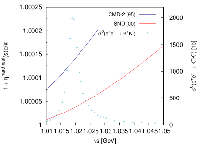
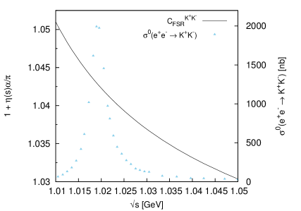
Figure 1: The effect of final state radiation in the K+Ksuperscript𝐾superscript𝐾K^{+}K^{-} channel in the ϕitalic-ϕ\phi resonance region. Left panel: the fully inclusive FSR correction η(s)𝜂𝑠\eta(s). Right panel: hard real radiation ηhard,real(s)superscript𝜂hardreal𝑠\eta^{\rm hard,real}(s), estimated with accolinearity cuts used in the two analyses [25, 26]. The e+eK+Ksuperscript𝑒superscript𝑒superscript𝐾superscript𝐾e^{+}e^{-}\rightarrow K^{+}K^{-} cross section is also plotted for reference.

In the case of the K+Ksuperscript𝐾superscript𝐾K^{+}K^{-} channel, by far the largest contribution to aμsubscript𝑎𝜇a_{\mu} and ΔαΔ𝛼\Delta\alpha (and their errors) comes from the energy region of the ϕitalic-ϕ\phi peak, where the phase space for real radiation is severely restricted. While the calculation of real radiation accounting for all experimental cuts would be very complicated and beyond the scope of this work, an estimate can easily be made based on equation (2.5), by relating ΛΛ\Lambda to the cuts in the photon accolinearity given in individual experimental analyses. In Figure 1, the result for the fully inclusive correction η(s)𝜂𝑠\eta(s) (left panel) is compared to the estimates for the real hard radiation, where ηhard,real(s)superscript𝜂hardreal𝑠\eta^{\rm hard,real}(s) (right panel) now depends on the accolinearity cuts as given by the two experimental analyses depicted. Clearly, at and around the ϕitalic-ϕ\phi peak, phase space restrictions strongly suppress any hard real radiation and using the inclusive correction would lead to an overestimate of the possible effects. Given the small size of both the possible correction in the ϕitalic-ϕ\phi region and the contribution of the K+Ksuperscript𝐾superscript𝐾K^{+}K^{-} channel above the ϕitalic-ϕ\phi to both mean value and error of aμsubscript𝑎𝜇a_{\mu} and ΔαΔ𝛼\Delta\alpha, no correction or additional error estimate due to FSR is now applied in the K+Ksuperscript𝐾superscript𝐾K^{+}K^{-} channel. For the neutral kaon channel, hard photon radiation (which would resolve the quark charges) is similarly suppressed and no FSR correction or additional error are applied in this channel also.

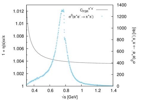
The situation is different in the two pion channel. A study similar to the two kaon channel showed that in principle larger contributions from real radiation of the order of the inclusive correction can arise. However, these contributions are strongly dependent on the cut applied in equation (2.5) and would require a more detailed, measurement-by-measurement analysis, which is beyond the scope of this work. In addition, for many of the data sets the required detailed information is not available. Therefore, in sets which are understood to not include the full FSR corrections, the fully inclusive correction (as shown in Figure 2) is applied to the respective measurements.
Refer to caption
Figure 2: The behaviour of the inclusive FSR correction, η(s)𝜂𝑠\eta(s), for the process e+eπ+πsuperscript𝑒superscript𝑒superscript𝜋superscript𝜋e^{+}e^{-}\rightarrow\pi^{+}\pi^{-}. The e+eπ+πsuperscript𝑒superscript𝑒superscript𝜋superscript𝜋e^{+}e^{-}\rightarrow\pi^{+}\pi^{-} cross section is also plotted for reference.

In the π+πsuperscript𝜋superscript𝜋\pi^{+}\pi^{-} data combination, recent sets from radiative return, where additional photons are part of the leading order cross section and are studied in detail as part of the analyses, have now become dominant. Therefore, the impact of the fully inclusive FSR correction to older sets is suppressed for both mean value and error in comparison to previous analyses. The procedure to determine the corresponding error estimate is discussed in the next chapter below, whilst resulting numbers are given in Section 3.1, which contains the detailed analysis of the π+πsuperscript𝜋superscript𝜋\pi^{+}\pi^{-} channel.

For the sub-leading, multi-hadron channels, there are, at present, no equivalent FSR calculations. Depending on the experimental analysis, they are (at least to some extent) estimated by Monte Carlo (MC) simulation and contribute to the systematic uncertainties.444In the recent work [27], a version of the MC program Carlomat [28] is discussed, which includes real photon radiation in multi-hadron channels. This could be used to further study the FSR effects. However, for many data sets, it is far from clear to which extent FSR effects are included in the systematic errors. Therefore, possible effects are accounted for by applying an additional uncertainty determined as a fraction of the respective contribution.

2.1.3 Estimating extra uncertainty due to radiative corrections

As in [7, 8, 9], extra uncertainties are estimated whenever additional radiative corrections are applied. This is done, first and foremost, to account for any under- or over-correction that may occur due to a lack of information concerning the treatment of radiative corrections in the experimental analyses. However, these radiative correction uncertainties also account for any possibly incorrect treatment in the analyses, e.g. missed FSR or inconsistent subtraction of VP contributions. This is especially true for older data, where there is very little or even no information at all regarding how the data have been treated.

In each channel, the difference ΔaμvpΔsuperscriptsubscript𝑎𝜇vp\Delta a_{\mu}^{\rm vp} between the estimates of aμsubscript𝑎𝜇a_{\mu} with and without additional VP corrections is determined. For the uncertainty due to VP, one third of the shift

δaμvp=13Δaμvp𝛿superscriptsubscript𝑎𝜇vp13Δsuperscriptsubscript𝑎𝜇vp\delta a_{\mu}^{\rm vp}=\frac{1}{3}\Delta a_{\mu}^{\rm vp}\, (2.6)

is taken. This is reduced from one half in [9], safe in the knowledge that the KNT18 VP routine [14], which is determined iteratively in a self-constistent way, is accurate to the level of a permille when correcting the cross section and that newer data sets are commonly undressed of VP effects by the experiment with a modern routine.

For the extra uncertainties due to FSR, there are now no contributions from the K+Ksuperscript𝐾superscript𝐾K^{+}K^{-} and KS0KL0subscriptsuperscript𝐾0𝑆subscriptsuperscript𝐾0𝐿K^{0}_{S}K^{0}_{L} channels (see the discussion above). For the π+πsuperscript𝜋superscript𝜋\pi^{+}\pi^{-} channel, the full difference between the estimates of aμπ+πsuperscriptsubscript𝑎𝜇superscript𝜋superscript𝜋a_{\mu}^{\pi^{+}\pi^{-}} with and without additional FSR corrections is taken as the FSR uncertainty. For all other channels, including the inclusive data combination above 1.937 GeV, a fraction of 1% of the respective cross section is applied as the uncertainty.

The numerical estimates of all additional radiative correction uncertainties are given in the respective sections for the individual channels. The same procedures are applied in the calculation of the contributions to ΔαhadΔsubscript𝛼had\Delta\alpha_{\rm had}.

2.2 Data combination

The combination of σ0(e+e\sigma^{0}(e^{+}e^{-}\rightarrow hadrons) data and its corresponding uncertainty has undergone a great deal of scrutiny since [9]. This has been due to the ever increasing amount of data that have become available and due to a better understanding of the treatment of correlated uncertainties that are now a prominent feature of many cross section measurements. In [9], covariance matrices in the π+πsuperscript𝜋superscript𝜋\pi^{+}\pi^{-} channel from BaBar [29] and KLOE [18, 19] for statistical and systematic uncertainties had already been included based on the method of fitted renormalisation factors. In the following, a new method for the combination of σhad0subscriptsuperscript𝜎0had\sigma^{0}_{\rm had} data is introduced, which will allow to fully take into account all correlated uncertainties.

2.2.1 Clustering data points

Within each hadronic channel, data points from different experiments are assigned to clusters (see [9, 7, 8] for details).555The effect that different clusterings have on the χmin2/d.o.f.formulae-sequencesubscriptsuperscript𝜒2mindof\chi^{2}_{\rm min}/{\rm d.o.f.} of the fit, the resulting aμhad,VPsuperscriptsubscript𝑎𝜇hadVPa_{\mu}^{\rm had,VP} value and its error has been discussed in detail in [9]. In this work, the clustering algorithm has been improved. It is universal for all different channels and only differs in the assigned maximum cluster size δ𝛿\delta (and δressubscript𝛿res\delta_{\rm res}, a maximum cluster size applicable at individual narrow resonances). A scan over δ𝛿\delta (and δressubscript𝛿res\delta_{\rm res} if applicable) is performed to determine a suitable clustering configuration which must avoid both over- and under-clustering. Too wide or overpopulated clusters would effectively lead to a re-binning of data points from individual experiments and risk loss of information, while a too narrow clustering would result, in the extreme, in an erratic point-to-point representation of the cross section and no gain in the accuracy. The preferred configuration is then chosen based on the global χmin2/d.o.f.formulae-sequencesubscriptsuperscript𝜒2mindof\chi^{2}_{\rm min}/{\rm d.o.f.} and the uncertainty on aμhad,VPsuperscriptsubscript𝑎𝜇hadVPa_{\mu}^{\rm had,VP}, combined with checks by eye of the resulting spectral function.

2.2.2 Fitting data

The previous analyses [9, 7, 8] employed a non-linear χ2superscript𝜒2\chi^{2}-minimisation utilising fitted renormalisation factors as nuisance parameters that represented the energy independent systematic uncertainties. Although a powerful method, recent literature [30] (see also [31]) have highlighted the possibility that an incorrect treatment of multiplicative normalisation uncertainties in a χ2superscript𝜒2\chi^{2} minimisation can incur a systematic bias (see chapter 4 of [30]). In addition, although the non-linear χ2superscript𝜒2\chi^{2}-minimisation used in [9] was adjusted to include covariance matrices, the method’s reliance on fitting energy independent renormalisation factors prevented the use of correlated uncertainties to their full capacity. As recent precise data, specifically radiative return measurements in the π+πsuperscript𝜋superscript𝜋\pi^{+}\pi^{-} and K+Ksuperscript𝐾superscript𝐾K^{+}K^{-} channels, have been released with energy dependent uncertainties and non-trivial bin-to-bin correlations for both the statistical and systematic uncertainties, the fit procedure had to be modified to allow the full use of all available correlations in a bias-free approach. Therefore, instead of fitting renormalisation factors (nuisance parameters), an iterative fit procedure as advocated in [30] has been adopted, which re-initialises the full covariance matrices at each iteration step and, consequently, avoids bias.

Previously, in [9, 7, 8], a constant cross section had been assumed across the width of each cluster. In this work, the fitted cross section values at the cluster centres are obtained from the iterative χ2superscript𝜒2\chi^{2}-minimisation where the cross section is taken to be linear between adjacent cluster centres. This allows for a more stable fit and is consistent with the trapezoidal rule integration utilised for the aμhad,VPsuperscriptsubscript𝑎𝜇hadVPa_{\mu}^{\rm had,VP} and ΔαhadΔsubscript𝛼had\Delta\alpha_{\rm had} integrals. If data points at energies s=Ei(m)𝑠superscriptsubscript𝐸𝑖𝑚\sqrt{s}=E_{i}^{(m)} are combined into cluster m𝑚m, then the weighted average of the cross section value Rmsubscript𝑅𝑚R_{m} and energy Emsubscript𝐸𝑚E_{m} for the cluster centre are

Rm=[i=1N(m)Ri(m)(dR~i(m))2][i=1N(m)1(dR~i(m))2]1subscript𝑅𝑚delimited-[]subscriptsuperscriptsuperscript𝑁𝑚𝑖1superscriptsubscript𝑅𝑖𝑚superscriptdsuperscriptsubscript~𝑅𝑖𝑚2superscriptdelimited-[]subscriptsuperscriptsuperscript𝑁𝑚𝑖11superscriptdsuperscriptsubscript~𝑅𝑖𝑚21R_{m}=\left[\sum^{N^{(m)}}_{i=1}\frac{R_{i}^{(m)}}{\left(\text{d}\tilde{R}_{i}^{(m)}\right)^{2}}\right]\left[\sum^{N^{(m)}}_{i=1}\frac{1}{\left(\text{d}\tilde{R}_{i}^{(m)}\right)^{2}}\right]^{-1} (2.7)

and

Em=[i=1N(m)Ei(m)(dR~i(m))2][i=1N(m)1(dR~i(m))2]1,subscript𝐸𝑚delimited-[]subscriptsuperscriptsuperscript𝑁𝑚𝑖1superscriptsubscript𝐸𝑖𝑚superscriptdsuperscriptsubscript~𝑅𝑖𝑚2superscriptdelimited-[]subscriptsuperscriptsuperscript𝑁𝑚𝑖11superscriptdsuperscriptsubscript~𝑅𝑖𝑚21E_{m}=\left[\sum^{N^{(m)}}_{i=1}\frac{E_{i}^{(m)}}{\left(\text{d}\tilde{R}_{i}^{(m)}\right)^{2}}\right]\left[\sum^{N^{(m)}}_{i=1}\frac{1}{\left(\text{d}\tilde{R}_{i}^{(m)}\right)^{2}}\right]^{-1}\,, (2.8)

where Ri(m)superscriptsubscript𝑅𝑖𝑚R_{i}^{(m)} is the cross section value of data point i𝑖i contributing to cluster m𝑚m, N(m)superscript𝑁𝑚N^{(m)} is the total number of data points contributing to cluster m𝑚m and

dR~i(m)=(dRi;stat(m))2+(dRi;sys(m))2.dsuperscriptsubscript~𝑅𝑖𝑚superscriptdsubscriptsuperscript𝑅𝑚𝑖stat2superscriptdsubscriptsuperscript𝑅𝑚𝑖sys2\text{d}\tilde{R}_{i}^{(m)}=\sqrt{(\text{d}R^{(m)}_{i;\ \text{stat}})^{2}+(\text{d}R^{(m)}_{i;\ \text{sys}})^{2}}\,. (2.9)

dRi;stat(m)dsubscriptsuperscript𝑅𝑚𝑖stat\text{d}R^{(m)}_{i;\ \text{stat}} and dRi;sys(m)dsubscriptsuperscript𝑅𝑚𝑖sys\text{d}R^{(m)}_{i;\ \text{sys}} denote the absolute statistical and systematic uncertainties, respectively. With a linear cross section now assumed, if data point i𝑖i belongs to cluster m𝑚m and Ei(m)>Emsubscriptsuperscript𝐸𝑚𝑖subscript𝐸𝑚E^{(m)}_{i}>E_{m}, then its interpolant cross section value misuperscriptsubscript𝑚𝑖\mathcal{R}_{m}^{i} is given by

mi+=Rm+(Ei(m)Em)(Em+1Em)(Rm+1Rm),superscriptsubscript𝑚limit-from𝑖subscript𝑅𝑚superscriptsubscript𝐸𝑖𝑚subscript𝐸𝑚subscript𝐸𝑚1subscript𝐸𝑚subscript𝑅𝑚1subscript𝑅𝑚\mathcal{R}_{m}^{i+}=R_{m}+\frac{(E_{i}^{(m)}-E_{m})}{(E_{m+1}-E_{m})}(R_{m+1}-R_{m})\,, (2.10)

where the ++ indicates that Ei(m)>Emsubscriptsuperscript𝐸𝑚𝑖subscript𝐸𝑚E^{(m)}_{i}>E_{m}. If, on the other hand, Ei(m)<Emsubscriptsuperscript𝐸𝑚𝑖subscript𝐸𝑚E^{(m)}_{i}<E_{m} then

mi=Rm1+(Ei(m)Em1)(EmEm1)(RmRm1),superscriptsubscript𝑚limit-from𝑖subscript𝑅𝑚1superscriptsubscript𝐸𝑖𝑚subscript𝐸𝑚1subscript𝐸𝑚subscript𝐸𝑚1subscript𝑅𝑚subscript𝑅𝑚1\mathcal{R}_{m}^{i-}=R_{m-1}+\frac{(E_{i}^{(m)}-E_{m-1})}{(E_{m}-E_{m-1})}(R_{m}-R_{m-1})\,, (2.11)

where the - indicates that Ei(m)<Emsuperscriptsubscript𝐸𝑖𝑚subscript𝐸𝑚E_{i}^{(m)}<E_{m}. For data points at the borders where no interpolation is possible, misuperscriptsubscript𝑚𝑖\mathcal{R}_{m}^{i} is found by linear extrapolation.

A covariance matrix is constructed for the combination which contains all the uncertainty and correlation information of all data points. Using the covariance matrix as defined by the data alone could result in bias (see [32, 33]). The covariance matrix is therefore redefined at each step of the iteration using the fitted Rmsubscript𝑅𝑚R_{m} values. Convergence of the iteration is observed in this work to occur after only a few steps.

The covariance matrix 𝐂(i(m),j(n))𝐂superscript𝑖𝑚superscript𝑗𝑛{\bf C}\big{(}i^{(m)},j^{(n)}\big{)} is given as the sum of the statistical covariance matrix Cstat(i(m),j(n))superscriptCstatsuperscript𝑖𝑚superscript𝑗𝑛{\rm C}^{\rm stat}\big{(}i^{(m)},j^{(n)}\big{)} and the systematic covariance matrix Csys(i(m),j(n))superscriptCsyssuperscript𝑖𝑚superscript𝑗𝑛{\rm C}^{\rm sys}\big{(}i^{(m)},j^{(n)}\big{)}. At each stage of the iteration, it is defined as

𝐂I(i(m),j(n))=Cstat(i(m),j(n))+Csys(i(m),j(n))Ri(m)Rj(n)mi,(I1)nj,(I1),subscript𝐂𝐼superscript𝑖𝑚superscript𝑗𝑛superscriptCstatsuperscript𝑖𝑚superscript𝑗𝑛superscriptCsyssuperscript𝑖𝑚superscript𝑗𝑛superscriptsubscript𝑅𝑖𝑚superscriptsubscript𝑅𝑗𝑛superscriptsubscript𝑚𝑖𝐼1superscriptsubscript𝑛𝑗𝐼1{\bf C}_{I}\big{(}i^{(m)},j^{(n)}\big{)}={\text{C}}^{\text{stat}}\big{(}i^{(m)},j^{(n)}\big{)}+\frac{{\text{C}}^{\text{sys}}\big{(}i^{(m)},j^{(n)}\big{)}}{R_{i}^{(m)}R_{j}^{(n)}}\mathcal{R}_{m}^{i,(I-1)}\mathcal{R}_{n}^{j,(I-1)}\,, (2.12)

where the quantities mi,Isuperscriptsubscript𝑚𝑖𝐼\mathcal{R}_{m}^{i,I} and nj,Isuperscriptsubscript𝑛𝑗𝐼\mathcal{R}_{n}^{j,I} are the interpolant cross sections given by either equation (2.10) or (2.11) and I𝐼I denotes the iteration number of the fit. This is then used as input into the now linear χ2superscript𝜒2\chi^{2}-function,

χI2=i=1Ntotj=1Ntot(Ri(m)mi,I)𝐂I1(i(m),j(n))(Rj(n)nj,I),subscriptsuperscript𝜒2𝐼subscriptsuperscriptsubscript𝑁tot𝑖1subscriptsuperscriptsubscript𝑁tot𝑗1superscriptsubscript𝑅𝑖𝑚superscriptsubscript𝑚𝑖𝐼superscriptsubscript𝐂𝐼1superscript𝑖𝑚superscript𝑗𝑛superscriptsubscript𝑅𝑗𝑛superscriptsubscript𝑛𝑗𝐼\chi^{2}_{I}=\sum^{N_{\mathrm{tot}}}_{i=1}\sum^{N_{\mathrm{tot}}}_{j=1}\big{(}R_{i}^{(m)}-\mathcal{R}_{m}^{i,I}\big{)}{\bf C}_{I}^{-1}\big{(}i^{(m)},j^{(n)}\big{)}\big{(}R_{j}^{(n)}-\mathcal{R}_{n}^{j,I}\big{)}\,, (2.13)

where Ntotsubscript𝑁totN_{\mathrm{tot}} is the total number of contributing data points and 𝐂I1(i(m),j(n))superscriptsubscript𝐂𝐼1superscript𝑖𝑚superscript𝑗𝑛{\bf C}_{I}^{-1}\big{(}i^{(m)},j^{(n)}\big{)} is simply the inverse of the covariance matrix defined in equation (2.12). Performing the minimisation yields a system of linear equations

j=1Ntot[(Rj(n)nj,I)miRa]VI1(m(i),n(j))=0,i=1,,Ntot,\sum^{N_{\mathrm{tot}}}_{j=1}\Biggr{[}\big{(}R_{j}^{(n)}-\mathcal{R}_{n}^{j,I}\big{)}\frac{\partial\mathcal{R}_{m}^{i}}{\partial R_{a}}\Biggr{]}V_{I}^{-1}\big{(}m^{(i)},n^{(j)}\big{)}=0\ ,\hskip 14.22636pti=1,...,N_{\mathrm{tot}}\,, (2.14)

where,

VI1(m(i),n(j))=i=1N(m)j=1N(n)𝐂I1(i(m),j(n)).superscriptsubscript𝑉𝐼1superscript𝑚𝑖superscript𝑛𝑗subscriptsuperscriptsuperscript𝑁𝑚𝑖1subscriptsuperscriptsuperscript𝑁𝑛𝑗1superscriptsubscript𝐂𝐼1superscript𝑖𝑚superscript𝑗𝑛V_{I}^{-1}\big{(}m^{(i)},n^{(j)}\big{)}=\sum^{N^{(m)}}_{i=1}\sum^{N^{(n)}}_{j=1}{\bf C}_{I}^{-1}\big{(}i^{(m)},j^{(n)}\big{)}\,. (2.15)

The solution to this yields the cluster centres Rmsubscript𝑅𝑚R_{m} and the covariance matrix VI(m,n)subscript𝑉𝐼𝑚𝑛V_{I}\big{(}m,n\big{)} which describes the correlation between the errors dRmdsubscript𝑅𝑚{\rm d}R_{m} and dRndsubscript𝑅𝑛{\rm d}R_{n}. As in equations (2.10) and (2.11), the term njsuperscriptsubscript𝑛𝑗\mathcal{R}_{n}^{j} is to be taken as either nj+superscriptsubscript𝑛limit-from𝑗\mathcal{R}_{n}^{j+}, if Ej(n)>Ensuperscriptsubscript𝐸𝑗𝑛subscript𝐸𝑛E_{j}^{(n)}>E_{n}, or njsuperscriptsubscript𝑛limit-from𝑗\mathcal{R}_{n}^{j-}, if Ej(n)<Ensuperscriptsubscript𝐸𝑗𝑛subscript𝐸𝑛E_{j}^{(n)}<E_{n}. Subsequently, if Ei(m)>Emsuperscriptsubscript𝐸𝑖𝑚subscript𝐸𝑚E_{i}^{(m)}>E_{m}, then

miRa|Ei(m)>Em=mi+Ra=(1(Ei(m)Em)(Em+1Em))δma+(Ei(m)Em)(Em+1Em)δm+1,a\frac{\partial\mathcal{R}_{m}^{i}}{\partial R_{a}}\Biggr{|}_{E_{i}^{(m)}>E_{m}}\ =\ \frac{\partial\mathcal{R}_{m}^{i+}}{\partial R_{a}}\ =\ \biggr{(}1-\frac{(E_{i}^{(m)}-E_{m})}{(E_{m+1}-E_{m})}\biggr{)}\delta_{ma}+\frac{(E_{i}^{(m)}-E_{m})}{(E_{m+1}-E_{m})}\delta_{m+1,a} (2.16)

and, if Ei(m)<Emsuperscriptsubscript𝐸𝑖𝑚subscript𝐸𝑚E_{i}^{(m)}<E_{m}, then

miRa|Ei(m)<Em=miRa=(1(Ei(m)Em1)(EmEm1))δm1,a+(Ei(m)Em1)(EmEm1)δma,\frac{\partial\mathcal{R}_{m}^{i}}{\partial R_{a}}\Biggr{|}_{E_{i}^{(m)}<E_{m}}\ =\ \frac{\partial\mathcal{R}_{m}^{i-}}{\partial R_{a}}\ =\ \biggr{(}1-\frac{(E_{i}^{(m)}-E_{m-1})}{(E_{m}-E_{m-1})}\biggr{)}\delta_{m-1,a}+\frac{(E_{i}^{(m)}-E_{m-1})}{(E_{m}-E_{m-1})}\delta_{ma}\,, (2.17)

where δ𝛿\delta denotes the usual Kronecker delta.

In [30], it was stated that for the fit of parton distribution functions, convergence is expected to occur after very few iterations, which is also observed here. The final result includes the total output covariance matrix V(m,n)𝑉𝑚𝑛V(m,n) which, as in [9], is inflated according to the local χmin2/d.o.f.formulae-sequencesubscriptsuperscript𝜒2mindof\chi^{2}_{\rm min}/{\rm d.o.f.} for each cluster if χmin2/d.o.f.>1\chi^{2}_{\rm min}/{\rm d.o.f.}>1. This is done in order to account for any tensions between the data. The use of the full covariance matrix allows for the inclusion of any-and-all uncertainties and correlations that may exist between the measurements. The flexibility to now make use of fully energy dependent uncertainties ensures that the appropriate influence of the correlations is incorporated into the determination of the cluster centres, Rmsubscript𝑅𝑚R_{m}, with the correct propagation of all experimental errors to the g2𝑔2g-2 uncertainty.

Note that, for all channels, the differences between the old and the new data combination procedures are small and lead to changes of aμhad,VPsuperscriptsubscript𝑎𝜇hadVPa_{\mu}^{\rm had,VP} well within the quoted errors. Importantly, combining data which have only global normalisation uncertainties results in negligible differences between [9] and this work, indicating that previous results were largely unaffected by the potential bias issue.

2.2.3 Integration

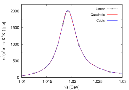
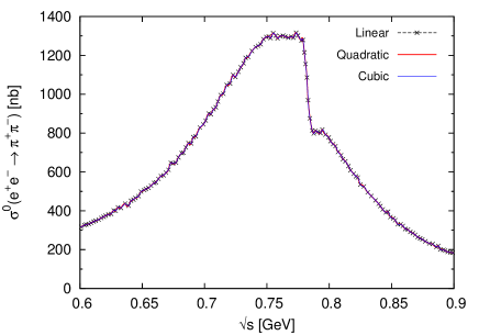
As in [9, 7, 8], the data are integrated using a trapezoidal rule integral in order to obtain aμhad,VPsuperscriptsubscript𝑎𝜇hadVPa_{\mu}^{\rm had,VP} and ΔαhadΔsubscript𝛼had\Delta\alpha_{\rm had}. In principle, the use of the trapezoidal rule integral could lead to unreliable results due to the form of the kernel function or at narrow resonances if data are sparse. However, with the current density of cross section measurements, especially in the dominant hadronic channels, the differences between trapezoidal rule integration and any higher order polynomial approximation are consequently small and of no concern. This can be seen in the plots in Figure 3.
Refer to caption
(a) The ρω𝜌𝜔\rho-\omega resonance region of the π+πsuperscript𝜋superscript𝜋\pi^{+}\pi^{-} channel.
Refer to caption
(b) The ϕitalic-ϕ\phi resonance region of the K+Ksuperscript𝐾superscript𝐾K^{+}K^{-} channel.
Figure 3: The differences observed using linear, quadratic and cubic integration routines in prominent resonance regions in the π+πsuperscript𝜋superscript𝜋\pi^{+}\pi^{-} and K+Ksuperscript𝐾superscript𝐾K^{+}K^{-} channels.

The calculation of the uncertainty of aμhad,VPsuperscriptsubscript𝑎𝜇hadVPa_{\mu}^{\rm had,VP} and ΔαhadΔsubscript𝛼had\Delta\alpha_{\rm had} has been modified to improve the determination of the error contribution at the integral boundaries. Should the upper or lower integral boundary, Easubscript𝐸𝑎E_{a}, with energy Em<Ea<Em+1subscript𝐸𝑚subscript𝐸𝑎subscript𝐸𝑚1E_{m}<E_{a}<E_{m+1} and cross section value Rm<Ra<Rm+1subscript𝑅𝑚subscript𝑅𝑎subscript𝑅𝑚1R_{m}<R_{a}<R_{m+1}, be found by linear interpolation (or extrapolation if it is necessary to extend the integral boundaries), then the output covariance matrix V(m,n)𝑉𝑚𝑛V\big{(}m,n\big{)} is interpolated accordingly using the standard error propagation formula

V(a,b)=mnRaRmV(m,n)RbRn,𝑉𝑎𝑏subscript𝑚subscript𝑛subscript𝑅𝑎subscript𝑅𝑚𝑉𝑚𝑛subscript𝑅𝑏subscript𝑅𝑛V\big{(}a,b\big{)}=\sum_{m}\sum_{n}\frac{\partial R_{a}}{\partial R_{m}}V\big{(}m,n\big{)}\frac{\partial R_{b}}{\partial R_{n}}\,, (2.18)

where m𝑚m, n𝑛n run over all clusters, b𝑏b is a label for any energy Ebsubscript𝐸𝑏E_{b} and V(b,a)=V(a,b)𝑉𝑏𝑎𝑉𝑎𝑏V\big{(}b,a\big{)}=V\big{(}a,b\big{)}.

3 Determining aμhad,VPsuperscriptsubscript𝑎𝜇hadVPa_{\mu}^{\rm had,VP} and Δαhad(MZ2)Δsubscript𝛼hadsuperscriptsubscript𝑀𝑍2\Delta\alpha_{\rm had}(M_{Z}^{2})

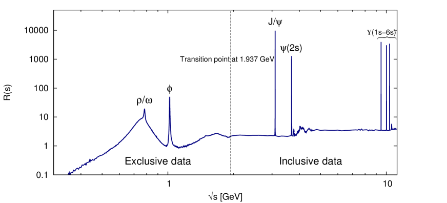
The following section summarises the data combination and estimates of aμhad,LOVPsuperscriptsubscript𝑎𝜇hadLOVPa_{\mu}^{\rm had,\,LO\,VP} and Δαhad(MZ2)Δsubscript𝛼hadsuperscriptsubscript𝑀𝑍2\Delta\alpha_{\rm had}(M_{Z}^{2}) from the leading and major sub-leading hadronic final states. All contributions from exclusive hadronic channels are evaluated up to 1.9371.9371.937 GeV, which is the chosen transition point between the sum of exclusive channels and the inclusive R𝑅R-ratio data in this work. This is discussed in detail in Section 3.6.1. Each contribution to aμhad,LOVPsuperscriptsubscript𝑎𝜇hadLOVPa_{\mu}^{\rm had,\,LO\,VP} is quoted with its respective statistical (stat) uncertainty, systematic (sys) uncertainty, VP (vp) correction uncertainty and FSR (fsr) correction uncertainty individually. This is followed by the contribution with a total (tot) uncertainty, determined from the individual sources added in quadrature,

aμhad,LOVPsuperscriptsubscript𝑎𝜇hadLOVP\displaystyle a_{\mu}^{\rm had,\,LO\,VP} =aμhad,LOVP±(δaμhad,LOVP)stat±(δaμhad,LOVP)sys±(δaμhad,LOVP)vp±(δaμhad,LOVP)fsrabsentplus-or-minussuperscriptsubscript𝑎𝜇hadLOVPsubscript𝛿superscriptsubscript𝑎𝜇hadLOVPstatsubscript𝛿superscriptsubscript𝑎𝜇hadLOVPsyssubscript𝛿superscriptsubscript𝑎𝜇hadLOVPvpsubscript𝛿superscriptsubscript𝑎𝜇hadLOVPfsr\displaystyle=a_{\mu}^{\rm had,\,LO\,VP}\pm(\delta a_{\mu}^{\rm had,\,LO\,VP})_{\rm stat}\pm(\delta a_{\mu}^{\rm had,\,LO\,VP})_{\rm sys}\pm(\delta a_{\mu}^{\rm had,\,LO\,VP})_{\rm vp}\pm(\delta a_{\mu}^{\rm had,\,LO\,VP})_{\rm fsr}
=aμhad,LOVP±(δaμhad,LOVP)tot.absentplus-or-minussuperscriptsubscript𝑎𝜇hadLOVPsubscript𝛿superscriptsubscript𝑎𝜇hadLOVPtot\displaystyle=a_{\mu}^{\rm had,\,LO\,VP}\pm(\delta a_{\mu}^{\rm had,\,LO\,VP})_{\rm tot}\,. (3.1)

All results for aμsubscript𝑎𝜇a_{\mu} are given in units 1010superscript101010^{-10}. For the contributions to Δαhad(MZ2)Δsubscript𝛼hadsuperscriptsubscript𝑀𝑍2\Delta\alpha_{\rm had}(M_{Z}^{2}), only the mean value with the corresponding total uncertainty,

Δαhad(MZ2)=Δαhad(MZ2)±(δΔαhad(MZ2))tot,Δsubscript𝛼hadsuperscriptsubscript𝑀𝑍2plus-or-minusΔsubscript𝛼hadsuperscriptsubscript𝑀𝑍2subscript𝛿Δsubscript𝛼hadsuperscriptsubscript𝑀𝑍2tot\Delta\alpha_{\rm had}(M_{Z}^{2})=\Delta\alpha_{\rm had}(M_{Z}^{2})\pm(\delta\Delta\alpha_{\rm had}(M_{Z}^{2}))_{\rm tot}\,, (3.2)

is quoted and all results are given in units 104superscript10410^{-4}. In both cases, uncertainties include all available correlations and local χ2superscript𝜒2\chi^{2} inflation as discussed in Section 2.2.2. In the following, unless stated explicitly, only those data sets that are new additions since [9], or those that have undergone studies that are mentioned in the text, are discussed and referenced. All other contributing data sets are referenced in [7, 8, 9].

3.1 π+πsuperscript𝜋superscript𝜋\pi^{+}\pi^{-} channel

The π+πsuperscript𝜋superscript𝜋\pi^{+}\pi^{-} channel is by far the most important contribution to aμhad,VPsuperscriptsubscript𝑎𝜇hadVPa_{\mu}^{\rm had,\,VP}, dominating both its mean value and uncertainty. With twenty-six data sets totalling almost one thousand data points, it is also the largest individual data combination. Two new radiative return measurements from the KLOE collaboration [34] and the BESIII collaboration [35] in the important ρ𝜌\rho region have greatly improved the estimate of this final state. The new data from the KLOE collaboration (KLOE12) agree well with both other measurements by KLOE (KLOE08 [18] and KLOE10 [19]). The three measurements are, in part, highly correlated, necessitating the construction of full statistical and systematic covariance matrices to be used in any combination of these data. This has been achieved in the separate work [17], where all details regarding the correlations, the resulting combination of the KLOE data and a comparison with other experimental measurements of σππ(γ)subscript𝜎𝜋𝜋𝛾\sigma_{\pi\pi(\gamma)} are presented. These covariance matrices are used here as input in the full π+πsuperscript𝜋superscript𝜋\pi^{+}\pi^{-} combination in order to fully incorporate the correlation information of the KLOE data as an influence on both the estimate of aμπ+πsuperscriptsubscript𝑎𝜇superscript𝜋superscript𝜋a_{\mu}^{\pi^{+}\pi^{-}} and its uncertainty.

Refer to caption
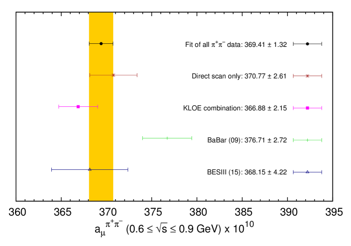
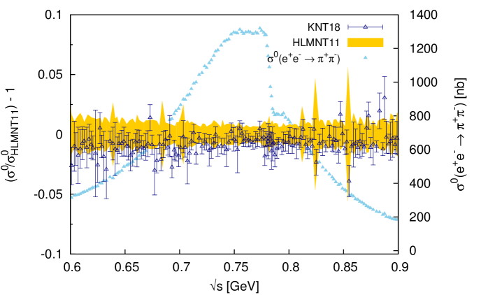
Figure 4: The comparison of the integration of the individual radiative return measurements and the combination of direct scan π+πsuperscript𝜋superscript𝜋\pi^{+}\pi^{-} measurements between 0.6s0.90.6𝑠0.90.6\leq\sqrt{s}\leq 0.9 GeV.

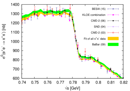
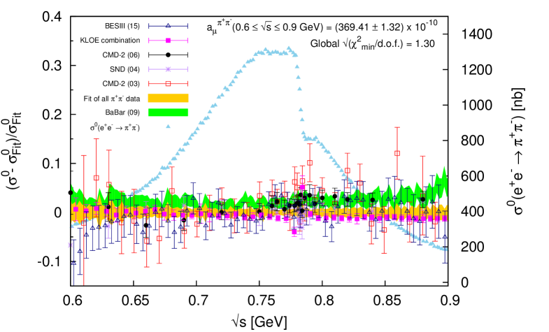
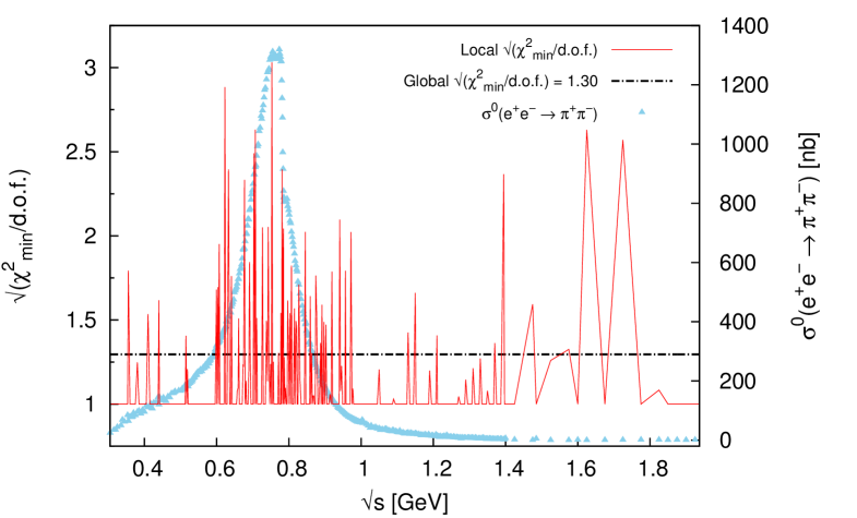
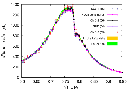
The BESIII measurement in the ρ𝜌\rho resonance region (again with full statistical and systematic covariance matrices) allows for an in-depth comparison of the existing radiative return measurements already contributing to the π+πsuperscript𝜋superscript𝜋\pi^{+}\pi^{-} channel, namely the three measurements by the KLOE collaboration and the finely binned measurement from the BaBar collaboration [29]. In [9], details were given regarding tension between the KLOE and BaBar measurements, where the BaBar data were considerably higher. As is evident from Figure 4, tension exists between the BaBar data and all other contributing data in the dominant ρ𝜌\rho region. When considering this along with the plots of the resulting cross section in Figure 5, it is clear that the new BESIII data agrees well with the KLOE data and the full π+πsuperscript𝜋superscript𝜋\pi^{+}\pi^{-} combination. Interestingly, however, it is in better agreement with the BaBar data at the peak of the resonance where the cross section is largest. Although BaBar still influences with an increase, the agreement between the other radiative return measurements and the direct scan data largely compensates for this effect. This is demonstrated by Figure 6, with the combination clearly favouring the other measurements. Tension between data sets, however, still exists and is reflected in the local χ2superscript𝜒2\chi^{2} error inflation, which results in an 15%similar-toabsentpercent15\sim 15\% increase in the uncertainty of aμπ+πsuperscriptsubscript𝑎𝜇superscript𝜋superscript𝜋a_{\mu}^{\pi^{+}\pi^{-}}. The effect of this energy dependent error inflation is shown in Figure 7, where the difference in using a local scaling of the error instead of a global one is clearly visible. Tensions arise in particular in the ρ𝜌\rho resonance region, where the cross section is large.
Refer to caption
(a)
Refer to caption
(b)
Figure 5: Contributing data in the ρ𝜌\rho resonance region of the π+πsuperscript𝜋superscript𝜋\pi^{+}\pi^{-} channel plotted against the new fit of all data (left panel), with an enlargement of the ρω𝜌𝜔\rho-\omega interference region (right panel).
Refer to caption
Figure 6: The relative difference of the radiative return and important direct scan data sets contributing to aμπ+πsuperscriptsubscript𝑎𝜇superscript𝜋superscript𝜋a_{\mu}^{\pi^{+}\pi^{-}} and the fit of all data. For comparison, the individual sets have been normalised against the fit and have been plotted in the ρ𝜌\rho region. The light green band represents the BaBar data and their errors (statistical and systematic, added in quadrature). The yellow band represents the full data combination which incorporates all correlated statistical and systematic uncertainties. However, the width of the yellow band simply displays the square root of the diagonal elements of the total output covariance matrix of the fit.
Refer to caption
Figure 7: The effect of the local χ2superscript𝜒2\chi^{2} inflation and the overall global χmin2/d.o.f.formulae-sequencesubscriptsuperscript𝜒2mindof\chi^{2}_{\rm min}/{\rm d.o.f.} in the π+πsuperscript𝜋superscript𝜋\pi^{+}\pi^{-} channel, which is plotted against the e+eπ+πsuperscript𝑒superscript𝑒superscript𝜋superscript𝜋e^{+}e^{-}\rightarrow\pi^{+}\pi^{-} cross section for reference.

The full combination of all π+πsuperscript𝜋superscript𝜋\pi^{+}\pi^{-} data is found to give

aμπ+π[0.305s1.937 GeV]superscriptsubscript𝑎𝜇superscript𝜋superscript𝜋delimited-[]0.305𝑠1.937 GeV\displaystyle a_{\mu}^{\pi^{+}\pi^{-}}[0.305\leq\sqrt{s}\leq 1.937\text{ GeV}] =502.97±1.14±1.59±0.06±0.14absentplus-or-minus502.971.141.590.060.14\displaystyle=502.97\pm 1.14\pm 1.59\pm 0.06\pm 0.14
=502.97±1.97absentplus-or-minus502.971.97\displaystyle=502.97\pm 1.97 (3.3)

and

Δαπ+π(MZ2)[0.305s1.937 GeV]=34.26±0.12.Δsubscript𝛼superscript𝜋superscript𝜋superscriptsubscript𝑀𝑍2delimited-[]0.305𝑠1.937 GeVplus-or-minus34.260.12\Delta\alpha_{\pi^{+}\pi^{-}}(M_{Z}^{2})[0.305\leq\sqrt{s}\leq 1.937\text{ GeV}]=34.26\pm 0.12\,. (3.4)

Although this value of aμπ+πsuperscriptsubscript𝑎𝜇superscript𝜋superscript𝜋a_{\mu}^{\pi^{+}\pi^{-}} stays well within the error estimate of [9], it exhibits a substantial decrease of the mean value. This has been attributed to the new data combination routine which allows for the full use of correlations in the determination of the mean value as well as the uncertainty and the inclusion of the new, precise radiative return data which suppresses the influence of BaBar in the ρ𝜌\rho resonance region.

In comparison with equation (3.3), the BaBar data alone in the same energy range give an estimate of aμπ+π(BaBar data only)=513.2±3.8superscriptsubscript𝑎𝜇superscript𝜋superscript𝜋BaBar data onlyplus-or-minus513.23.8a_{\mu}^{\pi^{+}\pi^{-}}(\text{BaBar data only})=513.2\pm 3.8. Should all available π+πsuperscript𝜋superscript𝜋\pi^{+}\pi^{-} data be combined using a simple weighted average as in equation (2.7), which only provides the error weighting to each cluster by its local uncertainty, the estimate for aμπ+πsuperscriptsubscript𝑎𝜇superscript𝜋superscript𝜋a_{\mu}^{\pi^{+}\pi^{-}} would be aμπ+π(Naive weighteda_{\mu}^{\pi^{+}\pi^{-}}(\text{Naive weighted} average)=509.1±2.9{\rm average})=509.1\pm 2.9. In this case, the estimate is strongly pulled up by the fine binning and high statistics of the BaBar data that dominate when no correlations are taken into account for the mean value. This difference of nearly 2σ2𝜎2\sigma when comparing to equation (3.3) indicates the importance of fully incorporating all available correlated uncertainties in any combination of the data.

The uncertainty has reduced by approximately one third. Again, this is due to the new, precise radiative return data which further dominate the π+πsuperscript𝜋superscript𝜋\pi^{+}\pi^{-} fit and the improvement of the overall combination which now fully incorporates the energy dependent correlations. In addition, the radiative corrections uncertainties have reduced since [9], as discussed in detail in Section 2.1.

3.2 π+ππ0superscript𝜋superscript𝜋superscript𝜋0\pi^{+}\pi^{-}\pi^{0} channel

Since [9], there has only been one new addition to the π+ππ0superscript𝜋superscript𝜋superscript𝜋0\pi^{+}\pi^{-}\pi^{0} channel [36]. This new data set improves this channel away from resonance, where previously only BaBar data [37] had provided a contribution of notable precision. Compared to [9], an additional change is applied to three separate data scans over the ϕitalic-ϕ\phi resonance in a measurement by CMD-2 [38], where the systematic uncertainties between the three scans are now taken to be fully correlated [39]. These changes, along with the new data combination routine, have resulted in an improved estimate of

aμπ+ππ0[0.66s1.937 GeV]superscriptsubscript𝑎𝜇superscript𝜋superscript𝜋superscript𝜋0delimited-[]0.66𝑠1.937 GeV\displaystyle a_{\mu}^{\pi^{+}\pi^{-}\pi^{0}}[0.66\leq\sqrt{s}\leq 1.937\text{ GeV}] =47.79±0.22±0.71±0.13±0.48absentplus-or-minus47.790.220.710.130.48\displaystyle=47.79\pm 0.22\pm 0.71\pm 0.13\pm 0.48
=47.79±0.89absentplus-or-minus47.790.89\displaystyle=47.79\pm 0.89 (3.5)

and

Δαπ+ππ0(MZ2)[0.66s1.937 GeV]=4.77±0.08.Δsubscript𝛼superscript𝜋superscript𝜋superscript𝜋0superscriptsubscript𝑀𝑍2delimited-[]0.66𝑠1.937 GeVplus-or-minus4.770.08\Delta\alpha_{\pi^{+}\pi^{-}\pi^{0}}(M_{Z}^{2})[0.66\leq\sqrt{s}\leq 1.937\text{ GeV}]=4.77\pm 0.08\,. (3.6)

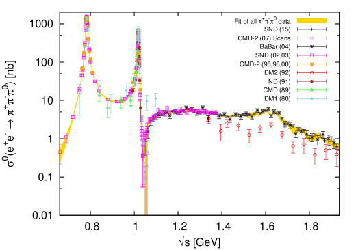
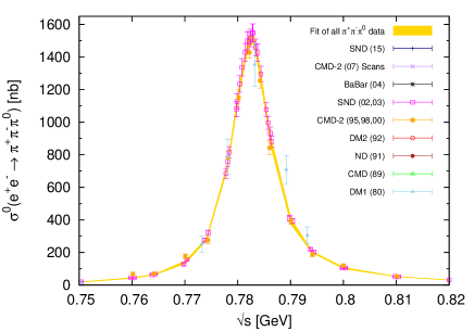
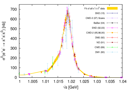
Figure 8 shows the full integral range of the data for the π+ππ0superscript𝜋superscript𝜋superscript𝜋0\pi^{+}\pi^{-}\pi^{0} cross section. Figure 9 shows an enlargement of the ω𝜔\omega and ϕitalic-ϕ\phi resonance regions in this channel.

Refer to caption
Figure 8: The cross section σ0(e+eπ+ππ0)superscript𝜎0superscript𝑒superscript𝑒superscript𝜋superscript𝜋superscript𝜋0\sigma^{0}(e^{+}e^{-}\rightarrow\pi^{+}\pi^{-}\pi^{0}) in the range 0.66s1.9370.66𝑠1.9370.66\leq\sqrt{s}\leq 1.937 GeV, where the prominent ω𝜔\omega and ϕitalic-ϕ\phi resonances are clearly visible.
Refer to caption
(a) The ω𝜔\omega resonance.
Refer to caption
(b) The ϕitalic-ϕ\phi resonance.
Figure 9: Enlargements of the resonance regions in the π+ππ0superscript𝜋superscript𝜋superscript𝜋0\pi^{+}\pi^{-}\pi^{0} final state.

3.3 4π4𝜋4\pi channels

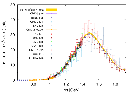
The π+ππ+πsuperscript𝜋superscript𝜋superscript𝜋superscript𝜋\pi^{+}\pi^{-}\pi^{+}\pi^{-} channel now includes two new additions since [9]. First, an improved statistics measurement by the BaBar collaboration in the range 0.6125s4.48750.6125𝑠4.48750.6125\leq\sqrt{s}\leq 4.4875 GeV [40] supersedes their previous measurement in this channel [41]. More recently, a data set by the CMD-3 collaboration in the range 0.92s1.060.92𝑠1.060.92\leq\sqrt{s}\leq 1.06 GeV [42] has been completed, which better resolves the interference pattern of the ϕπ+ππ+πitalic-ϕsuperscript𝜋superscript𝜋superscript𝜋superscript𝜋\phi\rightarrow\pi^{+}\pi^{-}\pi^{+}\pi^{-} transition that is clearly evident in the non-resonant cross section. In addition, the M3N thesis data [43] that are not published, but were previously included in this channel, are now discarded. With these changes,
Refer to caption
Figure 10: The cross section σ0(e+eπ+ππ+π)superscript𝜎0superscript𝑒superscript𝑒superscript𝜋superscript𝜋superscript𝜋superscript𝜋\sigma^{0}(e^{+}e^{-}\rightarrow\pi^{+}\pi^{-}\pi^{+}\pi^{-}) in the range 0.6125s1.9370.6125𝑠1.9370.6125\leq\sqrt{s}\leq 1.937 GeV.
Refer to caption
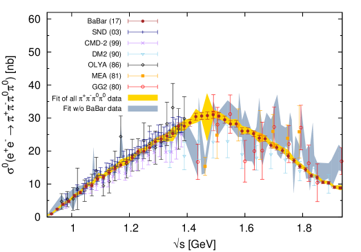
Figure 11: The cross section σ0(e+eπ+ππ0π0)superscript𝜎0superscript𝑒superscript𝑒superscript𝜋superscript𝜋superscript𝜋0superscript𝜋0\sigma^{0}(e^{+}e^{-}\rightarrow\pi^{+}\pi^{-}\pi^{0}\pi^{0}) in the range 0.850s1.9370.850𝑠1.9370.850\leq\sqrt{s}\leq 1.937 GeV.
aμπ+ππ+π[0.6125s1.937 GeV]superscriptsubscript𝑎𝜇superscript𝜋superscript𝜋superscript𝜋superscript𝜋delimited-[]0.6125𝑠1.937 GeV\displaystyle a_{\mu}^{\pi^{+}\pi^{-}\pi^{+}\pi^{-}}[0.6125\leq\sqrt{s}\leq 1.937\text{ GeV}] =14.87±0.02±0.13±0.03±0.15absentplus-or-minus14.870.020.130.030.15\displaystyle=14.87\pm 0.02\pm 0.13\pm 0.03\pm 0.15
=14.87±0.20absentplus-or-minus14.870.20\displaystyle=14.87\pm 0.20 (3.7)

and

Δαπ+ππ+π(MZ2)[0.6125s1.937 GeV]=4.02±0.05.Δsubscript𝛼superscript𝜋superscript𝜋superscript𝜋superscript𝜋superscriptsubscript𝑀𝑍2delimited-[]0.6125𝑠1.937 GeVplus-or-minus4.020.05\Delta\alpha_{\pi^{+}\pi^{-}\pi^{+}\pi^{-}}(M_{Z}^{2})[0.6125\leq\sqrt{s}\leq 1.937\text{ GeV}]=4.02\pm 0.05\,. (3.8)

Here, the mean value has increased since [9] largely due to the new BaBar data. The fitted cross section and data are displayed in Figure 10.

The picture for the π+ππ0π0superscript𝜋superscript𝜋superscript𝜋0superscript𝜋0\pi^{+}\pi^{-}\pi^{0}\pi^{0} final state has also improved, with a new measurement of this channel by BaBar [44] providing the only new data in this channel since 2003. As with the π+ππ+πsuperscript𝜋superscript𝜋superscript𝜋superscript𝜋\pi^{+}\pi^{-}\pi^{+}\pi^{-} channel, the M3N data [43] in this channel have been omitted. The estimate for this channel is

aμπ+ππ0π0[0.850s1.937 GeV]superscriptsubscript𝑎𝜇superscript𝜋superscript𝜋superscript𝜋0superscript𝜋0delimited-[]0.850𝑠1.937 GeV\displaystyle a_{\mu}^{\pi^{+}\pi^{-}\pi^{0}\pi^{0}}[0.850\leq\sqrt{s}\leq 1.937\text{ GeV}] =19.39±0.09±0.74±0.04±0.19absentplus-or-minus19.390.090.740.040.19\displaystyle=19.39\pm 0.09\pm 0.74\pm 0.04\pm 0.19
=19.39±0.78absentplus-or-minus19.390.78\displaystyle=19.39\pm 0.78 (3.9)

and

Δαπ+ππ0π0(MZ2)[0.850s1.937 GeV]=5.00±0.20,Δsubscript𝛼superscript𝜋superscript𝜋superscript𝜋0superscript𝜋0superscriptsubscript𝑀𝑍2delimited-[]0.850𝑠1.937 GeVplus-or-minus5.000.20\Delta\alpha_{\pi^{+}\pi^{-}\pi^{0}\pi^{0}}(M_{Z}^{2})[0.850\leq\sqrt{s}\leq 1.937\text{ GeV}]=5.00\pm 0.20\,, (3.10)

where there is clear improvement since [9]. The uncertainty contribution from π+ππ0π0superscript𝜋superscript𝜋superscript𝜋0superscript𝜋0\pi^{+}\pi^{-}\pi^{0}\pi^{0} is, however, still relatively large in comparison with its contribution to aμhad,LOVPsuperscriptsubscript𝑎𝜇hadLOVPa_{\mu}^{\rm had,\,LO\,VP} and ΔαhadΔsubscript𝛼had\Delta\alpha_{\rm had} and requires better new data. The new fit of the data for the bare cross section e+eπ+ππ0π0superscript𝑒superscript𝑒superscript𝜋superscript𝜋superscript𝜋0superscript𝜋0e^{+}e^{-}\rightarrow\pi^{+}\pi^{-}\pi^{0}\pi^{0} is shown in Figure 11. The fit without the new BaBar data is shown for comparison to highlight the large improvement this new data set provides.

3.4 KK¯𝐾¯𝐾K\bar{K} channels

Refer to caption
(a) Full range of the cross section σ0(e+eK+K)superscript𝜎0superscript𝑒superscript𝑒superscript𝐾superscript𝐾\sigma^{0}(e^{+}e^{-}\rightarrow K^{+}K^{-}).
Refer to caption
(b) The ϕitalic-ϕ\phi resonance.
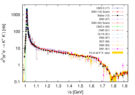
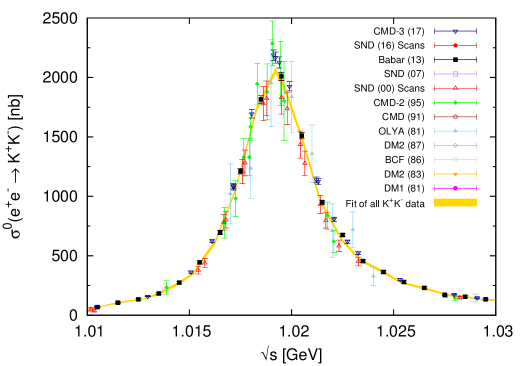
Figure 12: The cross section σ0(e+eK+K)superscript𝜎0superscript𝑒superscript𝑒superscript𝐾superscript𝐾\sigma^{0}(e^{+}e^{-}\rightarrow K^{+}K^{-}) in the range 0.9875s1.9370.9875𝑠1.9370.9875\leq\sqrt{s}\leq 1.937 GeV and an enlargement of the ϕitalic-ϕ\phi resonance. The large influence of the BaBar data (black squares) overwhelms the older data.

The K+Ksuperscript𝐾superscript𝐾K^{+}K^{-} channel now includes a precise and finely binned measurement by the BaBar collaboration, supplemented with full statistical and systematic covariance matrices [45]. This is the first and only example to date of the release of energy dependent, correlated uncertainties outside of the π+πsuperscript𝜋superscript𝜋\pi^{+}\pi^{-} channel and has an overwhelming influence on the data combination. There is also a new measurement in this channel of the ϕitalic-ϕ\phi resonance by the CMD-3 collaboration [46]. The existing CMD-2 scans in the same region [47] are omitted from this work as they suffer from an overestimation of the trigger efficiency for slow kaons [46] and are awaiting reanalysis[48]. In addition, two new scans by the SND collaboration measured at the tail of the ϕitalic-ϕ\phi and into the continuum are included [49]. The systematic uncertainties of these two scans, along with the existing two scans by SND [26], are considered to be fully correlated [39]. The combination of the available K+Ksuperscript𝐾superscript𝐾K^{+}K^{-} data now gives

aμK+K[0.9875s1.937 GeV]superscriptsubscript𝑎𝜇superscript𝐾superscript𝐾delimited-[]0.9875𝑠1.937 GeV\displaystyle a_{\mu}^{K^{+}K^{-}}[0.9875\leq\sqrt{s}\leq 1.937\text{ GeV}] =23.03±0.08±0.20±0.03±0.00absentplus-or-minus23.030.080.200.030.00\displaystyle=23.03\pm 0.08\pm 0.20\pm 0.03\pm 0.00
=23.03±0.22absentplus-or-minus23.030.22\displaystyle=23.03\pm 0.22 (3.11)

and

ΔαK+K(MZ2)[0.9875s1.937 GeV]=3.37±0.03,Δsubscript𝛼superscript𝐾superscript𝐾superscriptsubscript𝑀𝑍2delimited-[]0.9875𝑠1.937 GeVplus-or-minus3.370.03\Delta\alpha_{K^{+}K^{-}}(M_{Z}^{2})[0.9875\leq\sqrt{s}\leq 1.937\text{ GeV}]=3.37\pm 0.03\,, (3.12)

which exhibits an increase of the mean value of more than 1σ𝜎\sigma from the estimate in [9] attributed to the inclusion of the new BaBar and CMD-3 data. The cross section of the process e+eK+Ksuperscript𝑒superscript𝑒superscript𝐾superscript𝐾e^{+}e^{-}\rightarrow K^{+}K^{-} is displayed in Figure 12.

Refer to caption
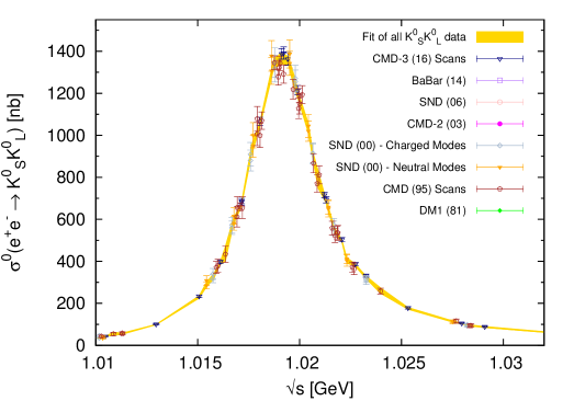
(a) Full range of the cross section σ0(e+eKS0KL0)superscript𝜎0superscript𝑒superscript𝑒subscriptsuperscript𝐾0𝑆subscriptsuperscript𝐾0𝐿\sigma^{0}(e^{+}e^{-}\rightarrow K^{0}_{S}K^{0}_{L}).
Refer to caption
(b) The ϕitalic-ϕ\phi resonance.
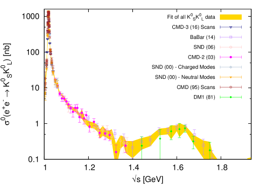
Figure 13: The cross section σ0(e+eKS0KL0)superscript𝜎0superscript𝑒superscript𝑒subscriptsuperscript𝐾0𝑆subscriptsuperscript𝐾0𝐿\sigma^{0}(e^{+}e^{-}\rightarrow K^{0}_{S}K^{0}_{L}) with an enlargement of the ϕitalic-ϕ\phi resonance.

The uncertainty has drastically improved since [9] with much of the change being due to a finer clustering over the ϕitalic-ϕ\phi resonance after the inclusion of the new high statistics BaBar data. Following from the discussion in Section 2.1.2, that there is now no FSR correction applied to this channel and, therefore, there is no extra radiative correction uncertainty due to FSR. It should also be noted that any FSR correction would result in an increase of aμK+Ksuperscriptsubscript𝑎𝜇superscript𝐾superscript𝐾a_{\mu}^{K^{+}K^{-}}, showing again the strong influence the new data have had in this channel to increase the mean value since [9], where previously an FSR correction was applied.

New data for the KS0KL0subscriptsuperscript𝐾0𝑆subscriptsuperscript𝐾0𝐿K^{0}_{S}K^{0}_{L} final state is included from the BaBar collaboration above the ϕitalic-ϕ\phi resonance [50] and from the CMD-3 collaboration on the ϕitalic-ϕ\phi [51]. Two existing measurements in this channel [26, 52] have multiple data scans of which the systematic uncertainties are now taken to be fully correlated [39]. This combination results in a contribution of

aμKS0KL0[1.00371s1.937 GeV]superscriptsubscript𝑎𝜇subscriptsuperscript𝐾0𝑆subscriptsuperscript𝐾0𝐿delimited-[]1.00371𝑠1.937 GeV\displaystyle a_{\mu}^{K^{0}_{S}K^{0}_{L}}[1.00371\leq\sqrt{s}\leq 1.937\text{ GeV}] =13.04±0.05±0.16±0.10±0.00absentplus-or-minus13.040.050.160.100.00\displaystyle=13.04\pm 0.05\pm 0.16\pm 0.10\pm 0.00
=13.04±0.19absentplus-or-minus13.040.19\displaystyle=13.04\pm 0.19 (3.13)

and

ΔαKS0KL0(MZ2)[1.00371s1.937 GeV]=1.77±0.03.Δsubscript𝛼subscriptsuperscript𝐾0𝑆subscriptsuperscript𝐾0𝐿superscriptsubscript𝑀𝑍2delimited-[]1.00371𝑠1.937 GeVplus-or-minus1.770.03\Delta\alpha_{K^{0}_{S}K^{0}_{L}}(M_{Z}^{2})[1.00371\leq\sqrt{s}\leq 1.937\text{ GeV}]=1.77\pm 0.03\,. (3.14)

Again, there is also no additional FSR correction uncertainty applied to this channel, with the reasoning in Section 2.1.2 enforced by the probability of photon emission being highly suppressed for a neutral final state and given the limited phase space. The cross section of the process e+eKS0KL0superscript𝑒superscript𝑒subscriptsuperscript𝐾0𝑆subscriptsuperscript𝐾0𝐿e^{+}e^{-}\rightarrow K^{0}_{S}K^{0}_{L} is displayed in Figure 13.

3.5 KK¯π𝐾¯𝐾𝜋K\bar{K}\pi and KK¯2π𝐾¯𝐾2𝜋K\bar{K}2\pi channels

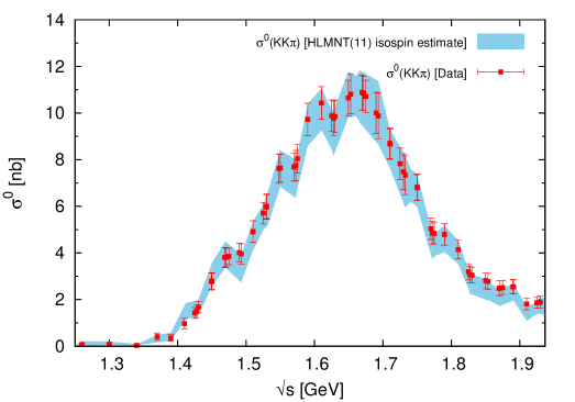
Since [9], the neutral final state KS0KL0π0subscriptsuperscript𝐾0𝑆subscriptsuperscript𝐾0𝐿superscript𝜋0K^{0}_{S}K^{0}_{L}\pi^{0} has been measured by BaBar [53] and SND [54], completing all modes that contribute to the KKπ𝐾𝐾𝜋KK\pi final state and removing the reliance on isospin for this channel (other than KS0KL0subscriptsuperscript𝐾0𝑆subscriptsuperscript𝐾0𝐿K^{0}_{S}\cong K^{0}_{L}). Therefore, the KKπ𝐾𝐾𝜋KK\pi cross section is now calculated using

σ(KKπ)𝜎𝐾𝐾𝜋\displaystyle\sigma(KK\pi) =σ(KS0K±π)+σ(KL0K±π)+σ(K+Kπ0)+σ(KS0KL0π0)absent𝜎subscriptsuperscript𝐾0𝑆superscript𝐾plus-or-minussuperscript𝜋minus-or-plus𝜎subscriptsuperscript𝐾0𝐿superscript𝐾plus-or-minussuperscript𝜋minus-or-plus𝜎superscript𝐾superscript𝐾superscript𝜋0𝜎subscriptsuperscript𝐾0𝑆subscriptsuperscript𝐾0𝐿superscript𝜋0\displaystyle=\sigma(K^{0}_{S}K^{\pm}\pi^{\mp})+\sigma(K^{0}_{L}K^{\pm}\pi^{\mp})+\sigma(K^{+}K^{-}\pi^{0})+\sigma(K^{0}_{S}K^{0}_{L}\pi^{0})
2σ(KS0K±π)+σ(K+Kπ0)+σ(KS0KL0π0),similar-to-or-equalsabsent2𝜎subscriptsuperscript𝐾0𝑆superscript𝐾plus-or-minussuperscript𝜋minus-or-plus𝜎superscript𝐾superscript𝐾superscript𝜋0𝜎subscriptsuperscript𝐾0𝑆subscriptsuperscript𝐾0𝐿superscript𝜋0\displaystyle\simeq 2\sigma(K^{0}_{S}K^{\pm}\pi^{\mp})+\sigma(K^{+}K^{-}\pi^{0})+\sigma(K^{0}_{S}K^{0}_{L}\pi^{0})\,, (3.15)

resulting in a contribution of

aμKKπ[1.260s1.937 GeV]superscriptsubscript𝑎𝜇𝐾𝐾𝜋delimited-[]1.260𝑠1.937 GeV\displaystyle a_{\mu}^{KK\pi}[1.260\leq\sqrt{s}\leq 1.937\text{ GeV}] =2.71±0.05±0.11±0.01±0.01absentplus-or-minus2.710.050.110.010.01\displaystyle=2.71\pm 0.05\pm 0.11\pm 0.01\pm 0.01
=2.71±0.12absentplus-or-minus2.710.12\displaystyle=2.71\pm 0.12 (3.16)

and

ΔαKKπ(MZ2)[1.260s1.937 GeV]=0.89±0.04.Δsubscript𝛼𝐾𝐾𝜋superscriptsubscript𝑀𝑍2delimited-[]1.260𝑠1.937 GeVplus-or-minus0.890.04\Delta\alpha_{KK\pi}(M_{Z}^{2})[1.260\leq\sqrt{s}\leq 1.937\text{ GeV}]=0.89\pm 0.04\,. (3.17)

In [9], the isospin estimate in the same energy range yielded,

aμKKπ(HLMNT11 isospin estimate)=2.65±0.14.superscriptsubscript𝑎𝜇𝐾𝐾𝜋HLMNT11 isospin estimateplus-or-minus2.650.14a_{\mu}^{KK\pi}(\text{HLMNT11 isospin estimate})=2.65\pm 0.14. (3.18)

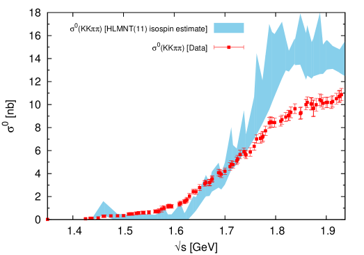
This good agreement between the HLMNT11 isospin estimate and the data-based approach in this analysis is also demonstrated in Figure 14.
Refer to caption
Figure 14: The measured cross section σ0(KKπ)superscript𝜎0𝐾𝐾𝜋\sigma^{0}(KK\pi) compared to the estimate from the previously used isospin relation.
Refer to caption
Figure 15: The cross section σ0(KKππ)superscript𝜎0𝐾𝐾𝜋𝜋\sigma^{0}(KK\pi\pi) compared to the previous estimate using isospin relations.

For KK2π𝐾𝐾2𝜋KK2\pi, BaBar have measured the previously missing modes KS0KL0π+πsubscriptsuperscript𝐾0𝑆subscriptsuperscript𝐾0𝐿superscript𝜋superscript𝜋K^{0}_{S}K^{0}_{L}\pi^{+}\pi^{-}, KS0KS0π+πsubscriptsuperscript𝐾0𝑆subscriptsuperscript𝐾0𝑆superscript𝜋superscript𝜋K^{0}_{S}K^{0}_{S}\pi^{+}\pi^{-} [50], KS0KL02π0subscriptsuperscript𝐾0𝑆subscriptsuperscript𝐾0𝐿2superscript𝜋0K^{0}_{S}K^{0}_{L}2\pi^{0} [53] and KS0K±ππ0subscriptsuperscript𝐾0𝑆superscript𝐾plus-or-minussuperscript𝜋minus-or-plussuperscript𝜋0K^{0}_{S}K^{\pm}\pi^{\mp}\pi^{0} [55], such that this contribution is now determined using

σ(KK2π)𝜎𝐾𝐾2𝜋\displaystyle\sigma(KK2\pi) =σ(K+Kπ0π0)+σ(K+Kπ+π)+σ(K0K0¯π+π)+σ(KS0KL02π0)absent𝜎superscript𝐾superscript𝐾superscript𝜋0superscript𝜋0𝜎superscript𝐾superscript𝐾superscript𝜋superscript𝜋𝜎superscript𝐾0¯superscript𝐾0superscript𝜋superscript𝜋𝜎subscriptsuperscript𝐾0𝑆subscriptsuperscript𝐾0𝐿2superscript𝜋0\displaystyle=\sigma(K^{+}K^{-}\pi^{0}\pi^{0})+\sigma(K^{+}K^{-}\pi^{+}\pi^{-})+\sigma(K^{0}\bar{K^{0}}\pi^{+}\pi^{-})+\sigma(K^{0}_{S}K^{0}_{L}2\pi^{0})
+σ(KS0K±ππ0)+σ(KL0K±ππ0)𝜎subscriptsuperscript𝐾0𝑆superscript𝐾plus-or-minussuperscript𝜋minus-or-plussuperscript𝜋0𝜎subscriptsuperscript𝐾0𝐿superscript𝐾plus-or-minussuperscript𝜋minus-or-plussuperscript𝜋0\displaystyle\ \ \ +\ \sigma(K^{0}_{S}K^{\pm}\pi^{\mp}\pi^{0})+\sigma(K^{0}_{L}K^{\pm}\pi^{\mp}\pi^{0})
σ(K+Kπ0π0)+σ(K+Kπ+π)+σ(K0K0¯π+π)+σ(KS0KL02π0)similar-to-or-equalsabsent𝜎superscript𝐾superscript𝐾superscript𝜋0superscript𝜋0𝜎superscript𝐾superscript𝐾superscript𝜋superscript𝜋𝜎superscript𝐾0¯superscript𝐾0superscript𝜋superscript𝜋𝜎subscriptsuperscript𝐾0𝑆subscriptsuperscript𝐾0𝐿2superscript𝜋0\displaystyle\simeq\sigma(K^{+}K^{-}\pi^{0}\pi^{0})+\sigma(K^{+}K^{-}\pi^{+}\pi^{-})+\sigma(K^{0}\bar{K^{0}}\pi^{+}\pi^{-})+\sigma(K^{0}_{S}K^{0}_{L}2\pi^{0})
+ 2σ(KS0K±ππ0).2𝜎subscriptsuperscript𝐾0𝑆superscript𝐾plus-or-minussuperscript𝜋minus-or-plussuperscript𝜋0\displaystyle\ \ \ +\ 2\sigma(K^{0}_{S}K^{\pm}\pi^{\mp}\pi^{0})\,. (3.19)

Here, again, it is assumed that KS0KL0subscriptsuperscript𝐾0𝑆subscriptsuperscript𝐾0𝐿K^{0}_{S}\cong K^{0}_{L} and, hence,

σ(K0K0¯π+π)𝜎superscript𝐾0¯superscript𝐾0superscript𝜋superscript𝜋\displaystyle\sigma(K^{0}\bar{K^{0}}\pi^{+}\pi^{-}) =σ(KS0KL0π+π)+σ(KS0KS0π+π)+σ(KL0KL0π+π)absent𝜎subscriptsuperscript𝐾0𝑆subscriptsuperscript𝐾0𝐿superscript𝜋superscript𝜋𝜎subscriptsuperscript𝐾0𝑆subscriptsuperscript𝐾0𝑆superscript𝜋superscript𝜋𝜎subscriptsuperscript𝐾0𝐿subscriptsuperscript𝐾0𝐿superscript𝜋superscript𝜋\displaystyle=\sigma(K^{0}_{S}K^{0}_{L}\pi^{+}\pi^{-})+\sigma(K^{0}_{S}K^{0}_{S}\pi^{+}\pi^{-})+\sigma(K^{0}_{L}K^{0}_{L}\pi^{+}\pi^{-})
σ(KS0KL0π+π)+2σ(KS0KS0π+π).similar-to-or-equalsabsent𝜎subscriptsuperscript𝐾0𝑆subscriptsuperscript𝐾0𝐿superscript𝜋superscript𝜋2𝜎subscriptsuperscript𝐾0𝑆subscriptsuperscript𝐾0𝑆superscript𝜋superscript𝜋\displaystyle\simeq\sigma(K^{0}_{S}K^{0}_{L}\pi^{+}\pi^{-})+2\sigma(K^{0}_{S}K^{0}_{S}\pi^{+}\pi^{-})\,. (3.20)

Therefore, the estimate in this channel is now found to be

aμKK2π[1.350s1.937 GeV]superscriptsubscript𝑎𝜇𝐾𝐾2𝜋delimited-[]1.350𝑠1.937 GeV\displaystyle a_{\mu}^{KK2\pi}[1.350\leq\sqrt{s}\leq 1.937\text{ GeV}] =1.93±0.03±0.07±0.01±0.01absentplus-or-minus1.930.030.070.010.01\displaystyle=1.93\pm 0.03\pm 0.07\pm 0.01\pm 0.01
=1.93±0.08absentplus-or-minus1.930.08\displaystyle=1.93\pm 0.08 (3.21)

and

ΔαKK2π(MZ2)[1.350s1.937 GeV]=0.75±0.03.Δsubscript𝛼𝐾𝐾2𝜋superscriptsubscript𝑀𝑍2delimited-[]1.350𝑠1.937 GeVplus-or-minus0.750.03\Delta\alpha_{KK2\pi}(M_{Z}^{2})[1.350\leq\sqrt{s}\leq 1.937\text{ GeV}]=0.75\pm 0.03\,. (3.22)

Comparing equation (3.5) with the HLMNT11 isospin estimate in the same energy range of

aμKK2π(HLMNT11 isospin estimate)=2.51±0.35superscriptsubscript𝑎𝜇𝐾𝐾2𝜋HLMNT11 isospin estimateplus-or-minus2.510.35a_{\mu}^{KK2\pi}(\text{HLMNT11 isospin estimate})=2.51\pm 0.35 (3.23)

and examining Figure 15, it is evident that the isospin relations provided a poor estimate of this final state. Using the data, KK2π𝐾𝐾2𝜋KK2\pi contributes a much smaller mean value with a greatly reduced uncertainty.

3.6 Inclusive R𝑅R-ratio data

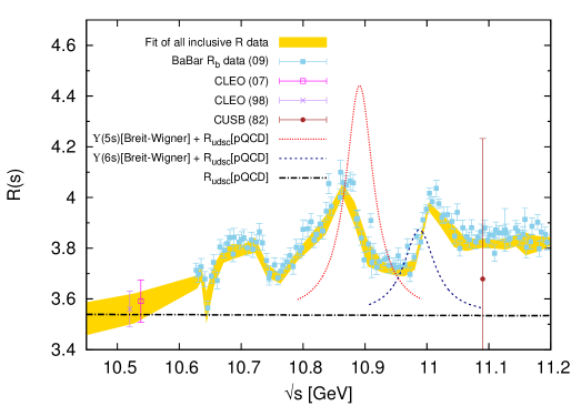
The combination of inclusive hadronic R𝑅R-ratio data between 1.937s11.21.937𝑠11.21.937\leq\sqrt{s}\leq 11.2 GeV has three new data additions since [9]. The first of these are the precise BaBar Rbsubscript𝑅𝑏R_{b} data between 10.54s11.2010.54𝑠11.2010.54\leq\sqrt{s}\leq 11.20 GeV [56], which must be deconvoluted of the effects from initial state radiation (ISR) and must have the radiative tails of the resonances from the Υ(1S4S)Υ1𝑆4𝑆\Upsilon(1S-4S) states removed (see [57]). These data are then added to the perturbative QCD (pQCD) estimate of Rudscsubscript𝑅𝑢𝑑𝑠𝑐R_{udsc} [58] to be included as an accurate data set in the inclusive channel in this region. The inclusion of the BaBar Rbsubscript𝑅𝑏R_{b} data is particularly beneficial as it resolves the resonances of the Υ(5S)Υ5𝑆\Upsilon(5S) and Υ(6S)Υ6𝑆\Upsilon(6S) states, removing the need to estimate these structures using a Breit-Wigner parametrisation as was done in [7, 8, 9]. These data are shown in Figure 16, together with the previously used incoherent sum of the resonance parametrisations which are clearly very different from the bb¯𝑏¯𝑏b\bar{b} cross section as measured by BaBar. Note that apart from the CLEO(98) data point [59] at 10.5210.5210.52 GeV, the CLEO(07) data point [60] at 10.53810.53810.538 GeV and the CUSB data point at 11.0911.0911.09 GeV [61], there are no other data in this bb¯𝑏¯𝑏b\bar{b} resonance region.

Refer to caption
Figure 16: The fit of inclusive R𝑅R data in the region of the newly included BaBar Rbsubscript𝑅𝑏R_{b} data, with the BaBar Rbsubscript𝑅𝑏R_{b} is shown as light blue markers. The resonance structures of the Υ(5S)Υ5𝑆\Upsilon(5S) and Υ(6S)Υ6𝑆\Upsilon(6S) states are clearly visible.
Refer to caption
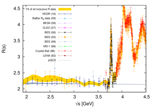
Figure 17: The combination of inclusive R𝑅R data in the region 1.937s4.501.937𝑠4.501.937\leq\sqrt{s}\leq 4.50 GeV. For comparison, the fit and the contributing data are plotted against the estimate of pQCD, represented by the dashed line and grey band.

The other new data are recent precise measurements by the KEDR collaboration: one set between 1.84s3.051.84𝑠3.051.84\leq\sqrt{s}\leq 3.05 GeV [62] and two scans in the energy range 3.12s3.723.12𝑠3.723.12\leq\sqrt{s}\leq 3.72 GeV [63]. For the latter, the systematic uncertainties are taken to be fully correlated [39]. The fit of the inclusive data in the range 1.937s3.801.937𝑠3.801.937\leq\sqrt{s}\leq 3.80 GeV is shown in Figure 17, which demonstrates the good agreement between KEDR and pQCD. In [9], the decision was made to use pQCD in the range 2.6s3.732.6𝑠3.732.6\leq\sqrt{s}\leq 3.73 GeV, where the quality of inclusive data was poor, with an error inflated according to the percentage errors of the inclusive BES data in this region [64]. With the new KEDR data [62, 63], the inclusive data combination is much improved, as shown in Figure 17. In this range, the data combination results in

aμhad,LOVP[inc.,2.60s3.73 GeV]=11.19±0.17,superscriptsubscript𝑎𝜇hadLOVPdelimited-[]inc.2.60𝑠3.73 GeVplus-or-minus11.190.17a_{\mu}^{\rm had,\,LO\,VP}[\text{inc.},2.60\leq\sqrt{s}\leq 3.73\text{ GeV}]=11.19\pm 0.17\ , (3.24)

whereas from pQCD (with an inflated uncertainty [9]), the estimate would be

aμhad,LOVP[pQCD,2.60s3.73 GeV]=10.82±0.35.superscriptsubscript𝑎𝜇hadLOVPdelimited-[]pQCD2.60𝑠3.73 GeVplus-or-minus10.820.35a_{\mu}^{\rm had,\,LO\,VP}[\text{pQCD},2.60\leq\sqrt{s}\leq 3.73\text{ GeV}]=10.82\pm 0.35\ . (3.25)

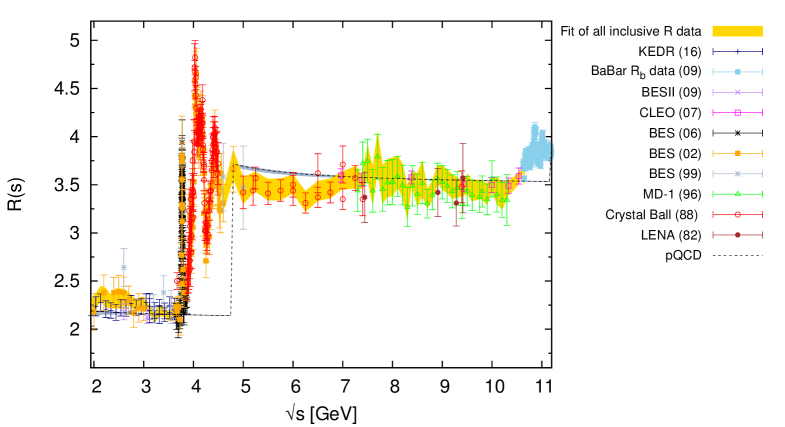
For the larger energy range 1.937s11.21.937𝑠11.21.937\leq\sqrt{s}\leq 11.2 GeV, the resulting data combination is displayed in Figure 18. As well as the differences observed between the data and pQCD below the charm threshold, the data above it (unchanged since[9]) also show a slight variation from the prediction of pQCD. Considering that with the new, precise KEDR data, the differences between the inclusive data and pQCD are not as large as previously and that this work is aiming at a predominantly data-driven analysis, the contributions in the entire inclusive data region are now estimated using the inclusive data alone. Hence, for this analysis, the contribution from the inclusive data is found to be

aμhad,LOVP[inc.,1.937s11.2 GeV]superscriptsubscript𝑎𝜇hadLOVPdelimited-[]inc.1.937𝑠11.2 GeV\displaystyle a_{\mu}^{\rm had,\,LO\,VP}[\text{inc.},1.937\leq\sqrt{s}\leq 11.2\text{ GeV}] =43.67±0.17±0.48±0.01±0.44absentplus-or-minus43.670.170.480.010.44\displaystyle=43.67\pm 0.17\pm 0.48\pm 0.01\pm 0.44
=43.67±0.67absentplus-or-minus43.670.67\displaystyle=43.67\pm 0.67 (3.26)

and

Δαhad(MZ2)[inc.,1.937s11.2 GeV]=82.82±1.05.Δsubscript𝛼hadsuperscriptsubscript𝑀𝑍2delimited-[]inc.1.937𝑠11.2 GeVplus-or-minus82.821.05\Delta\alpha_{\text{had}}(M_{Z}^{2})[\text{inc.},1.937\leq\sqrt{s}\leq 11.2\text{ GeV}]=82.82\pm 1.05\ . (3.27)
Refer to caption
Figure 18: Compilation of inclusive data in range 1.937s11.2 GeV1.937𝑠11.2 GeV1.937\leq\sqrt{s}\leq 11.2\text{ GeV}. The dashed line and surrounding grey band shows the estimate from pQCD for comparison. The yellow band represents the total uncertainty of the inclusive data combination.

3.6.1 Transition region between exclusive and inclusive data

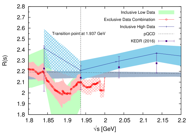
The transition region between the sum of exclusive states and the inclusive R𝑅R-ratio data is of interest and deserves re-examination. For the sum of exclusive channels, whilst many measurements extend to 2 GeV or beyond, with increasing energy the inclusion of more and more multi-hadronic final states is required to achieve a reliable estimate of the total hadronic cross section. Previously, in [9], the sum of exclusive data was used up to 2 GeV, which defined the transition point between the exclusive sum and the inclusive data combination. In this analysis, the new KEDR data [62] contribute two data points below 2 GeV, extending the lower boundary of the inclusive data down to 1.8411.8411.841 GeV (compared to 2 GeV in [9]) and providing an opportunity to reconsider the previous choice concerning the data input in this region.

From the lower boundary of the KEDR measurement up to 2 GeV, the resulting contributions to aμhad,LOVPsuperscriptsubscript𝑎𝜇hadLOVPa_{\mu}^{\rm had,\,LO\,VP} from the sum of exclusive states, the inclusive data combination and pQCD are given in Table 1. The integrated values of the inclusive data and pQCD agree within errors. However, the contribution from the sum of exclusive states disagrees with the estimates from both the inclusive data and pQCD, where the sum of exclusive provides a smaller contribution. This is particularly visible in Figure 19, where although the sum of exclusive states agrees with the two inclusive data points below 2 GeV at their respective energies, the combined sum of exclusive states is lower in general. This is largely attributed to the new data for the π+ππ0π0superscript𝜋superscript𝜋superscript𝜋0superscript𝜋0\pi^{+}\pi^{-}\pi^{0}\pi^{0} final state, where Figure 11 shows that these new data result in a clear reduction of the fitted cross section below 2 GeV.666Interestingly, as can be seen from Figure 19, the sum of exclusive states is in good agreement with the imprecise and, therefore, unused inclusive hadronic cross section data that exist between 1.43s2.001.43𝑠2.001.43\leq\sqrt{s}\leq 2.00 GeV. This is in contrast with the findings in the previous analyses [7, 8, 9], which observed that the inclusive data in this range were lower than the sum of exclusive states. Due to this effect, the previous transition point in [9] between the sum of exclusive states and the inclusive data combination at 2 GeV is no longer the preferred choice in this work, where it is clear from Figure 19 that these two different choices for the data input are largely incompatible at this point. A more natural choice for this transition point is now 1.937 GeV, where it can be seen from Figure 19 that all available data choices at this energy are in agreement within errors. This is further substantiated by Table 1, where the value for aμhad,LOVPsuperscriptsubscript𝑎𝜇hadLOVPa_{\mu}^{\rm had,\,LO\,VP} from the contribution from exclusive states below 1.937 GeV summed with the contribution from the inclusive data combination above 1.937 GeV is, within errors, in agreement with the integrated values of all other choices for the data input. Consequently, in this work, this is chosen to be the transition point between the sum of exclusive states and the inclusive R𝑅R-ratio data.

Input aμhad,LOVP[1.841s2.00GeV]×1010superscriptsubscript𝑎𝜇hadLOVPdelimited-[]1.841𝑠2.00GeVsuperscript1010a_{\mu}^{\rm had,\,LO\,VP}[1.841\leq\sqrt{s}\leq 2.00\ {\rm GeV}]\times 10^{10}
Exclusive sum 6.06±0.17plus-or-minus6.060.176.06\pm 0.17
Inclusive data 6.67±0.26plus-or-minus6.670.266.67\pm 0.26
pQCD 6.38±0.11plus-or-minus6.380.116.38\pm 0.11
Exclusive (<1.937absent1.937<1.937 GeV) + inclusive (>1.937absent1.937>1.937 GeV) 6.23±0.13plus-or-minus6.230.136.23\pm 0.13
Table 1: Comparison of results for aμhad,LOVP[1.841s2.00GeV]superscriptsubscript𝑎𝜇hadLOVPdelimited-[]1.841𝑠2.00GeVa_{\mu}^{\rm had,\,LO\,VP}[1.841\leq\sqrt{s}\leq 2.00\ {\rm GeV}] from the different available inputs in this region.
Refer to caption
Figure 19: The energy region between 1.8s2.21.8𝑠2.21.8\leq\sqrt{s}\leq 2.2 GeV where the fit of inclusive R ratio measurements (light blue band) replaces the sum of exclusive hadronic final states (red band) from 1.937 GeV to 2 GeV. The patterned light blue band and patterned red band show the continuation of the inclusive data combination below 1.937 GeV and the continuation of the exclusive sum above 1.937 GeV, respectively. The recent KEDR data are individually marked and included in the inclusive data fit. The light green band shows the data combination of old inclusive hadronic cross section data that exist between 1.43s2.001.43𝑠2.001.43\leq\sqrt{s}\leq 2.00 GeV, which were previously discussed in [9] and are not used due to their lack of precision. The estimate from pQCD is included for comparison as a dashed line with an error band which is dominated by the variation of the renormalisation scale μ𝜇\mu in the range 12s<μ<2s12𝑠𝜇2𝑠\frac{1}{2}\sqrt{s}<\mu<2\sqrt{s}.

3.7 Total contribution of aμhad,LOVPsuperscriptsubscript𝑎𝜇hadLOVPa_{\mu}^{\rm had,\,LO\,VP} and Δαhad(5)(MZ2)Δsuperscriptsubscript𝛼had5superscriptsubscript𝑀𝑍2\Delta\alpha_{\rm had}^{(5)}(M_{Z}^{2})

Channel Energy range (GeV) aμhad,LOVP×1010superscriptsubscript𝑎𝜇hadLOVPsuperscript1010a_{\mu}^{\rm had,\,LO\,VP}\times 10^{10} Δαhad(5)(MZ2)×104Δsuperscriptsubscript𝛼had5superscriptsubscript𝑀𝑍2superscript104\Delta\alpha_{\rm had}^{(5)}(M_{Z}^{2})\times 10^{4} New data
Chiral perturbation theory (ChPT) threshold contributions
π0γsuperscript𝜋0𝛾\pi^{0}\gamma mπs0.600subscript𝑚𝜋𝑠0.600\hphantom{00}m_{\pi}\leq\sqrt{s}\leq 0.600 0.12±0.01plus-or-minus0.120.01\hphantom{0}0.12\pm 0.01 0.00±0.00plus-or-minus0.000.00\hphantom{0}0.00\pm 0.00 -
π+πsuperscript𝜋superscript𝜋\pi^{+}\pi^{-} 2mπs0.3052subscript𝑚𝜋𝑠0.305\hphantom{0}2m_{\pi}\leq\sqrt{s}\leq 0.305 0.87±0.02plus-or-minus0.870.02\hphantom{0}0.87\pm 0.02 0.01±0.00plus-or-minus0.010.00\hphantom{0}0.01\pm 0.00 -
π+ππ0superscript𝜋superscript𝜋superscript𝜋0\pi^{+}\pi^{-}\pi^{0} 3mπs0.6603subscript𝑚𝜋𝑠0.660\hphantom{0}3m_{\pi}\leq\sqrt{s}\leq 0.660 0.01±0.00plus-or-minus0.010.00\hphantom{0}0.01\pm 0.00 0.00±0.00plus-or-minus0.000.00\hphantom{0}0.00\pm 0.00 -
ηγ𝜂𝛾\eta\gamma mηs0.660subscript𝑚𝜂𝑠0.660\hphantom{00}m_{\eta}\leq\sqrt{s}\leq 0.660 0.00±0.00plus-or-minus0.000.00\hphantom{0}0.00\pm 0.00 0.00±0.00plus-or-minus0.000.00\hphantom{0}0.00\pm 0.00 -
Data based channels (s1.937𝑠1.937\sqrt{s}\leq 1.937 GeV)
π0γsuperscript𝜋0𝛾\pi^{0}\gamma 0.600s1.3500.600𝑠1.3500.600\leq\sqrt{s}\leq 1.350 4.46±0.10plus-or-minus4.460.10\hphantom{0}4.46\pm 0.10 0.36±0.01plus-or-minus0.360.01\hphantom{0}0.36\pm 0.01 [65]
π+πsuperscript𝜋superscript𝜋\pi^{+}\pi^{-} 0.305s1.9370.305𝑠1.9370.305\leq\sqrt{s}\leq 1.937 502.97±1.97plus-or-minus502.971.97502.97\pm 1.97\hphantom{0} 34.26±0.12plus-or-minus34.260.1234.26\pm 0.12 [34, 35]
π+ππ0superscript𝜋superscript𝜋superscript𝜋0\pi^{+}\pi^{-}\pi^{0} 0.660s1.9370.660𝑠1.9370.660\leq\sqrt{s}\leq 1.937 47.79±0.89plus-or-minus47.790.8947.79\pm 0.89 4.77±0.08plus-or-minus4.770.08\hphantom{0}4.77\pm 0.08 [36]
π+ππ+πsuperscript𝜋superscript𝜋superscript𝜋superscript𝜋\pi^{+}\pi^{-}\pi^{+}\pi^{-} 0.613s1.9370.613𝑠1.9370.613\leq\sqrt{s}\leq 1.937 14.87±0.20plus-or-minus14.870.2014.87\pm 0.20 4.02±0.05plus-or-minus4.020.05\hphantom{0}4.02\pm 0.05 [40, 42]
π+ππ0π0superscript𝜋superscript𝜋superscript𝜋0superscript𝜋0\pi^{+}\pi^{-}\pi^{0}\pi^{0} 0.850s1.9370.850𝑠1.9370.850\leq\sqrt{s}\leq 1.937 19.39±0.78plus-or-minus19.390.7819.39\pm 0.78 5.00±0.20plus-or-minus5.000.20\hphantom{0}5.00\pm 0.20 [44]
(2π+2ππ0)no ηsubscript2superscript𝜋2superscript𝜋superscript𝜋0no 𝜂(2\pi^{+}2\pi^{-}\pi^{0})_{\text{no }\eta} 1.013s1.9371.013𝑠1.9371.013\leq\sqrt{s}\leq 1.937 0.99±0.09plus-or-minus0.990.09\hphantom{0}0.99\pm 0.09 0.33±0.03plus-or-minus0.330.03\hphantom{0}0.33\pm 0.03 -
3π+3π3superscript𝜋3superscript𝜋3\pi^{+}3\pi^{-} 1.313s1.9371.313𝑠1.9371.313\leq\sqrt{s}\leq 1.937 0.23±0.01plus-or-minus0.230.01\hphantom{0}0.23\pm 0.01 0.09±0.01plus-or-minus0.090.01\hphantom{0}0.09\pm 0.01 [66]
(2π+2π2π0)no ηωsubscript2superscript𝜋2superscript𝜋2superscript𝜋0no 𝜂𝜔(2\pi^{+}2\pi^{-}2\pi^{0})_{\text{no }\eta\omega} 1.322s1.9371.322𝑠1.9371.322\leq\sqrt{s}\leq 1.937 1.35±0.17plus-or-minus1.350.17\hphantom{0}1.35\pm 0.17 0.51±0.06plus-or-minus0.510.06\hphantom{0}0.51\pm 0.06 -
K+Ksuperscript𝐾superscript𝐾K^{+}K^{-} 0.988s1.9370.988𝑠1.9370.988\leq\sqrt{s}\leq 1.937 23.03±0.22plus-or-minus23.030.2223.03\pm 0.22 3.37±0.03plus-or-minus3.370.03\hphantom{0}3.37\pm 0.03 [45, 46, 49]
KS0KL0subscriptsuperscript𝐾0𝑆subscriptsuperscript𝐾0𝐿K^{0}_{S}K^{0}_{L} 1.004s1.9371.004𝑠1.9371.004\leq\sqrt{s}\leq 1.937 13.04±0.19plus-or-minus13.040.1913.04\pm 0.19 1.77±0.03plus-or-minus1.770.03\hphantom{0}1.77\pm 0.03 [50, 51]
KKπ𝐾𝐾𝜋KK\pi 1.260s1.9371.260𝑠1.9371.260\leq\sqrt{s}\leq 1.937 2.71±0.12plus-or-minus2.710.12\hphantom{0}2.71\pm 0.12 0.89±0.04plus-or-minus0.890.04\hphantom{0}0.89\pm 0.04 [53, 54]
KK2π𝐾𝐾2𝜋KK2\pi 1.350s1.9371.350𝑠1.9371.350\leq\sqrt{s}\leq 1.937 1.93±0.08plus-or-minus1.930.08\hphantom{0}1.93\pm 0.08 0.75±0.03plus-or-minus0.750.03\hphantom{0}0.75\pm 0.03 [50, 53, 55]
ηγ𝜂𝛾\eta\gamma 0.660s1.7600.660𝑠1.7600.660\leq\sqrt{s}\leq 1.760 0.70±0.02plus-or-minus0.700.02\hphantom{0}0.70\pm 0.02 0.09±0.00plus-or-minus0.090.00\hphantom{0}0.09\pm 0.00 [67]
ηπ+π𝜂superscript𝜋superscript𝜋\eta\pi^{+}\pi^{-} 1.091s1.9371.091𝑠1.9371.091\leq\sqrt{s}\leq 1.937 1.29±0.06plus-or-minus1.290.06\hphantom{0}1.29\pm 0.06 0.39±0.02plus-or-minus0.390.02\hphantom{0}0.39\pm 0.02 [68, 69]
(ηπ+ππ0)no ωsubscript𝜂superscript𝜋superscript𝜋superscript𝜋0no 𝜔(\eta\pi^{+}\pi^{-}\pi^{0})_{\text{no }\omega} 1.333s1.9371.333𝑠1.9371.333\leq\sqrt{s}\leq 1.937 0.60±0.15plus-or-minus0.600.15\hphantom{0}0.60\pm 0.15 0.21±0.05plus-or-minus0.210.05\hphantom{0}0.21\pm 0.05 [70]
η2π+2π𝜂2superscript𝜋2superscript𝜋\eta 2\pi^{+}2\pi^{-} 1.338s1.9371.338𝑠1.9371.338\leq\sqrt{s}\leq 1.937 0.08±0.01plus-or-minus0.080.01\hphantom{0}0.08\pm 0.01 0.03±0.00plus-or-minus0.030.00\hphantom{0}0.03\pm 0.00 -
ηω𝜂𝜔\eta\omega 1.333s1.9371.333𝑠1.9371.333\leq\sqrt{s}\leq 1.937 0.31±0.03plus-or-minus0.310.03\hphantom{0}0.31\pm 0.03 0.10±0.01plus-or-minus0.100.01\hphantom{0}0.10\pm 0.01 [70, 71]
ω(π0γ)π0\omega(\to\pi^{0}\gamma)\pi^{0} 0.920s1.9370.920𝑠1.9370.920\leq\sqrt{s}\leq 1.937 0.88±0.02plus-or-minus0.880.02\hphantom{0}0.88\pm 0.02 0.19±0.00plus-or-minus0.190.00\hphantom{0}0.19\pm 0.00 [72, 73]
ηϕ𝜂italic-ϕ\eta\phi 1.569s1.9371.569𝑠1.9371.569\leq\sqrt{s}\leq 1.937 0.42±0.03plus-or-minus0.420.03\hphantom{0}0.42\pm 0.03 0.15±0.01plus-or-minus0.150.01\hphantom{0}0.15\pm 0.01 -
ϕitalic-ϕabsent\phi\to unaccounted 0.988s1.0290.988𝑠1.0290.988\leq\sqrt{s}\leq 1.029 0.04±0.04plus-or-minus0.040.04\hphantom{0}0.04\pm 0.04 0.01±0.01plus-or-minus0.010.01\hphantom{0}0.01\pm 0.01 -
ηωπ0𝜂𝜔superscript𝜋0\eta\omega\pi^{0} 1.550s1.9371.550𝑠1.9371.550\leq\sqrt{s}\leq 1.937 0.35±0.09plus-or-minus0.350.09\hphantom{0}0.35\pm 0.09 0.14±0.04plus-or-minus0.140.04\hphantom{0}0.14\pm 0.04 [74]
η(npp)KK¯no ϕKK¯\eta(\rightarrow{\rm npp})K\bar{K}_{\text{no }\phi\rightarrow K\bar{K}} 1.569s1.9371.569𝑠1.9371.569\leq\sqrt{s}\leq 1.937 0.01±0.02plus-or-minus0.010.02\hphantom{0}0.01\pm 0.02 0.00±0.01plus-or-minus0.000.01\hphantom{0}0.00\pm 0.01 [75, 53]
pp¯𝑝¯𝑝p\bar{p} 1.890s1.9371.890𝑠1.9371.890\leq\sqrt{s}\leq 1.937 0.03±0.00plus-or-minus0.030.00\hphantom{0}0.03\pm 0.00 0.01±0.00plus-or-minus0.010.00\hphantom{0}0.01\pm 0.00 [76]
nn¯𝑛¯𝑛n\bar{n} 1.912s1.9371.912𝑠1.9371.912\leq\sqrt{s}\leq 1.937 0.03±0.01plus-or-minus0.030.01\hphantom{0}0.03\pm 0.01 0.01±0.00plus-or-minus0.010.00\hphantom{0}0.01\pm 0.00 [77]
Estimated contributions (s1.937𝑠1.937\sqrt{s}\leq 1.937 GeV)
(π+π3π0)no ηsubscriptsuperscript𝜋superscript𝜋3superscript𝜋0no 𝜂(\pi^{+}\pi^{-}3\pi^{0})_{\text{no }\eta} 1.013s1.9371.013𝑠1.9371.013\leq\sqrt{s}\leq 1.937 0.50±0.04plus-or-minus0.500.04\hphantom{0}0.50\pm 0.04 0.16±0.01plus-or-minus0.160.01\hphantom{0}0.16\pm 0.01 -
(π+π4π0)no ηsubscriptsuperscript𝜋superscript𝜋4superscript𝜋0no 𝜂(\pi^{+}\pi^{-}4\pi^{0})_{\text{no }\eta} 1.313s1.9371.313𝑠1.9371.313\leq\sqrt{s}\leq 1.937 0.21±0.21plus-or-minus0.210.21\hphantom{0}0.21\pm 0.21 0.08±0.08plus-or-minus0.080.08\hphantom{0}0.08\pm 0.08 -
KK3π𝐾𝐾3𝜋KK3\pi 1.569s1.9371.569𝑠1.9371.569\leq\sqrt{s}\leq 1.937 0.03±0.02plus-or-minus0.030.02\hphantom{0}0.03\pm 0.02 0.02±0.01plus-or-minus0.020.01\hphantom{0}0.02\pm 0.01 -
ω(npp)2π\omega(\rightarrow{\rm npp})2\pi 1.285s1.9371.285𝑠1.9371.285\leq\sqrt{s}\leq 1.937 0.10±0.02plus-or-minus0.100.02\hphantom{0}0.10\pm 0.02 0.03±0.01plus-or-minus0.030.01\hphantom{0}0.03\pm 0.01 -
ω(npp)3π\omega(\rightarrow{\rm npp})3\pi 1.322s1.9371.322𝑠1.9371.322\leq\sqrt{s}\leq 1.937 0.17±0.03plus-or-minus0.170.03\hphantom{0}0.17\pm 0.03 0.06±0.01plus-or-minus0.060.01\hphantom{0}0.06\pm 0.01 -
ω(npp)KK\omega(\rightarrow{\rm npp})KK 1.569s1.9371.569𝑠1.9371.569\leq\sqrt{s}\leq 1.937 0.00±0.00plus-or-minus0.000.00\hphantom{0}0.00\pm 0.00 0.00±0.00plus-or-minus0.000.00\hphantom{0}0.00\pm 0.00 -
ηπ+π2π0𝜂superscript𝜋superscript𝜋2superscript𝜋0\eta\pi^{+}\pi^{-}2\pi^{0} 1.338s1.9371.338𝑠1.9371.338\leq\sqrt{s}\leq 1.937 0.08±0.04plus-or-minus0.080.04\hphantom{0}0.08\pm 0.04 0.03±0.02plus-or-minus0.030.02\hphantom{0}0.03\pm 0.02 -
Other contributions (s>1.937𝑠1.937\sqrt{s}>1.937 GeV)
Inclusive channel 1.937s11.1991.937𝑠11.1991.937\leq\sqrt{s}\leq 11.199 43.67±0.67plus-or-minus43.670.6743.67\pm 0.67 82.82±1.05plus-or-minus82.821.0582.82\pm 1.05 [56, 62, 63]
J/ψ𝐽𝜓J/\psi - 6.26±0.19plus-or-minus6.260.19\hphantom{0}6.26\pm 0.19 7.07±0.22plus-or-minus7.070.22\hphantom{0}7.07\pm 0.22 -
ψsuperscript𝜓\psi^{\prime} - 1.58±0.04plus-or-minus1.580.04\hphantom{0}1.58\pm 0.04 2.51±0.06plus-or-minus2.510.06\hphantom{0}2.51\pm 0.06 -
Υ(1S4S)Υ1𝑆4𝑆\Upsilon(1S-4S) - 0.09±0.00plus-or-minus0.090.00\hphantom{0}0.09\pm 0.00 1.06±0.02plus-or-minus1.060.02\hphantom{0}1.06\pm 0.02 -
pQCD 11.199s11.199𝑠11.199\leq\sqrt{s}\leq\infty000 2.07±0.00plus-or-minus2.070.00\hphantom{0}2.07\pm 0.00 124.79±0.10plus-or-minus124.790.10124.79\pm 0.10\hphantom{0} -
Total mπssubscript𝑚𝜋𝑠m_{\pi}\leq\sqrt{s}\leq\infty0 693.26±2.46plus-or-minus693.262.46693.26\pm 2.46\hphantom{0} 276.11±1.11plus-or-minus276.111.11276.11\pm 1.11\hphantom{0} -
Table 2: Summary of the contributions to aμhad,LOVPsuperscriptsubscript𝑎𝜇hadLOVPa_{\mu}^{\rm had,\,LO\,VP} and Δαhad(5)(MZ2)Δsuperscriptsubscript𝛼had5superscriptsubscript𝑀𝑍2\Delta\alpha_{\rm had}^{(5)}(M_{Z}^{2}) calculated in this analysis. The first column indicates the hadronic final state or individual contribution, the second column gives the respective energy range of the contribution, the third column states the determined value of aμhad,LOVPsuperscriptsubscript𝑎𝜇hadLOVPa_{\mu}^{\rm had,\,LO\,VP}, the fourth column states the determined value of Δαhad(5)(MZ2)Δsuperscriptsubscript𝛼had5superscriptsubscript𝑀𝑍2\Delta\alpha_{\rm had}^{(5)}(M_{Z}^{2}) and the last column indicates any new data that have been included since [9]. The last row describes the total contribution obtained from the sum of the individual final states, with the uncertainties added in quadrature.
Refer to caption
(a) Fractional contributions to aμhad,LOVPsuperscriptsubscript𝑎𝜇hadLOVPa_{\mu}^{\rm had,\,LO\,VP}.
Refer to caption
(b) Fractional contributions to Δαhad(5)(MZ2)Δsuperscriptsubscript𝛼had5superscriptsubscript𝑀𝑍2\Delta\alpha_{\rm had}^{(5)}(M_{Z}^{2})
Figure 20: Pie charts showing the fractional contributions to the total mean value (left pie chart) and (error)2 (right pie chart) of both aμhad,LOVPsuperscriptsubscript𝑎𝜇hadLOVPa_{\mu}^{\rm had,\,LO\,VP} (upper panel) and Δαhad(5)(MZ2)Δsuperscriptsubscript𝛼had5superscriptsubscript𝑀𝑍2\Delta\alpha_{\rm had}^{(5)}(M_{Z}^{2}) (lower panel) from various energy intervals. The energy intervals for aμhad,LOVPsuperscriptsubscript𝑎𝜇hadLOVPa_{\mu}^{\rm had,\,LO\,VP} are defined by the boundaries mπsubscript𝑚𝜋m_{\pi}, 0.6, 0.9, 1.43, 2.0 and \infty GeV. For Δαhad(5)(MZ2)Δsuperscriptsubscript𝛼had5superscriptsubscript𝑀𝑍2\Delta\alpha_{\rm had}^{(5)}(M_{Z}^{2}), the intervals are defined by the energy boundaries mπsubscript𝑚𝜋m_{\pi}, 0.6, 0.9, 1.43, 2.0, 4.0, 11.2 and \infty GeV. In both cases, the (error)2 includes all experimental uncertainties (including all available correlations) and local χmin2/d.o.f.formulae-sequencesubscriptsuperscript𝜒2mindof\chi^{2}_{\rm min}/{\rm d.o.f.} inflation. The fractional contribution to the (error)2 from the radiative correction uncertainties are shown in black and indicated by ‘rad.’.
Refer to caption
(a) The hadronic R𝑅R-ratio.
Refer to caption
(b) The uncertainty of the hadronic R𝑅R-ratio.
Figure 21: Contributions to the total hadronic R𝑅R-ratio from the different final states (upper panel) and their uncertainties (lower panel) below 1.937 GeV. The full R𝑅R-ratio and its uncertainty is shown in light blue in each plot, respectively. Each final state is included as a new layer on top in decreasing order of the size of its contribution to aμhad,LOVPsuperscriptsubscript𝑎𝜇hadLOVPa_{\mu}^{\rm had,\,LO\,VP}.
Refer to caption
Figure 22: The resulting hadronic R𝑅R-ratio shown in the range mπs11.1985subscript𝑚𝜋𝑠11.1985m_{\pi}\leq\sqrt{s}\leq 11.1985 GeV, where the prominent resonances are labelled.

Table 2 lists all contributions from individual channels contributing to aμhad,LOVPsuperscriptsubscript𝑎𝜇hadLOVPa_{\mu}^{\rm had,\,LO\,VP}, with the corresponding total. From the sum of these contributions, the estimate for aμhad,LOVPsuperscriptsubscript𝑎𝜇hadLOVPa_{\mu}^{\rm had,\,LO\,VP} from this analysis is

aμhad,LOVPsuperscriptsubscript𝑎𝜇hadLOVP\displaystyle a_{\mu}^{\rm had,\,LO\,VP} =(693.26±1.19stat±2.01sys±0.22vp±0.71fsr)×1010absentplus-or-minus693.26subscript1.19statsubscript2.01syssubscript0.22vpsubscript0.71fsrsuperscript1010\displaystyle=(693.26\pm 1.19_{\rm stat}\pm 2.01_{\rm sys}\pm 0.22_{\rm vp}\pm 0.71_{\rm fsr})\times 10^{-10}
=(693.26±2.46tot)×1010,absentplus-or-minus693.26subscript2.46totsuperscript1010\displaystyle=(693.26\pm 2.46_{\rm tot})\times 10^{-10}\ , (3.28)

where the uncertainties include all available correlations and local χ2superscript𝜒2\chi^{2} inflation as discussed in Section 2.2.2. Using the same data compilation as described for the calculation of aμhad,LOVPsuperscriptsubscript𝑎𝜇hadLOVPa_{\mu}^{\rm had,\,LO\,VP}, the next-to-leading order (NLO) contribution to aμhad,VPsuperscriptsubscript𝑎𝜇hadVPa_{\mu}^{\rm had,VP} is determined here to be

aμhad,NLOVPsuperscriptsubscript𝑎𝜇hadNLOVP\displaystyle a_{\mu}^{\rm had,\,NLO\,VP} =(9.82±0.02stat±0.03sys±0.01vp±0.02fsr)×1010absentplus-or-minus9.82subscript0.02statsubscript0.03syssubscript0.01vpsubscript0.02fsrsuperscript1010\displaystyle=(-9.82\pm 0.02_{\rm stat}\pm 0.03_{\rm sys}\pm 0.01_{\rm vp}\pm 0.02_{\rm fsr})\times 10^{-10}
=(9.82±0.04tot)×1010.absentplus-or-minus9.82subscript0.04totsuperscript1010\displaystyle=(-9.82\pm 0.04_{\rm tot})\times 10^{-10}\ . (3.29)

The corresponding result for Δαhad(5)(MZ2)Δsuperscriptsubscript𝛼had5superscriptsubscript𝑀𝑍2\Delta\alpha_{\rm had}^{(5)}(M_{Z}^{2}) is

Δαhad(5)(MZ2)Δsuperscriptsubscript𝛼had5superscriptsubscript𝑀𝑍2\displaystyle\Delta\alpha_{\rm had}^{(5)}(M_{Z}^{2}) =(276.11±0.26stat±0.68sys±0.14vp±0.83fsr)×104absentplus-or-minus276.11subscript0.26statsubscript0.68syssubscript0.14vpsubscript0.83fsrsuperscript104\displaystyle=(276.11\pm 0.26_{\rm stat}\pm 0.68_{\rm sys}\pm 0.14_{\rm vp}\pm 0.83_{\rm fsr})\times 10^{-4}
=(276.11±1.11tot)×104,absentplus-or-minus276.11subscript1.11totsuperscript104\displaystyle=(276.11\pm 1.11_{\rm tot})\times 10^{-4}\ , (3.30)

where the superscript (5) indicates the contributions from all quark flavours except the top quark, which is added separately. In each case, the errors from the individual channels and sources of uncertainty are added in quadrature to determine the total error. The fractional contributions to the total mean value and uncertainty of both aμhad,LOVPsuperscriptsubscript𝑎𝜇hadLOVPa_{\mu}^{\rm had,\,LO\,VP} and Δαhad(5)(MZ2)Δsuperscriptsubscript𝛼had5superscriptsubscript𝑀𝑍2\Delta\alpha_{\rm had}^{(5)}(M_{Z}^{2}) from various energy intervals is shown in Figure 20. Here, the dominance of the energy region below 0.90.90.9 GeV for aμhad,LOVPsuperscriptsubscript𝑎𝜇hadLOVPa_{\mu}^{\rm had,\,LO\,VP} and its uncertainty is clearly evident, with this being predominantly due to the contributions from the π+πsuperscript𝜋superscript𝜋\pi^{+}\pi^{-} channel. Notably, the pie chart depicting the fractional contributions to the (error)2 of Δαhad(5)(MZ2)Δsuperscriptsubscript𝛼had5superscriptsubscript𝑀𝑍2\Delta\alpha_{\rm had}^{(5)}(M_{Z}^{2}) reveals how the uncertainty on this quantity is dominated by the contributions from the radiative correction uncertainties. Mostly, this large error contribution comes from the uncertainty due to possible FSR applied to the combination of inclusive data above 1.937 GeV discussed in Section 2.1.3. This, in particular, highlights the differences in the kernel functions of the respective dispersion integrals for aμhad,LOVPsuperscriptsubscript𝑎𝜇hadLOVPa_{\mu}^{\rm had,\,LO\,VP} and Δαhad(5)(MZ2)Δsuperscriptsubscript𝛼had5superscriptsubscript𝑀𝑍2\Delta\alpha_{\rm had}^{(5)}(M_{Z}^{2}), where contributions from higher energies have a larger influence on Δαhad(5)(MZ2)Δsuperscriptsubscript𝛼had5superscriptsubscript𝑀𝑍2\Delta\alpha_{\rm had}^{(5)}(M_{Z}^{2}) than on aμhad,LOVPsuperscriptsubscript𝑎𝜇hadLOVPa_{\mu}^{\rm had,\,LO\,VP}. If, instead of a data driven analysis, the region above 1.937 GeV was estimated using pQCD, it would effectively eliminate the impacting radiative correction uncertainties in this region. Figure 21 shows the contributions from all hadronic final states to the hadronic R𝑅R-ratio and its uncertainty below 1.937 GeV. Here, the individual final states are displayed separately as well as with the resulting total hadronic R𝑅R-ratio. The full compilation for the hadronic R𝑅R-ratio is shown in Figure 22. The data vector and corresponding covariance matrix of the hadronic R𝑅R-ratio in the range mπs11.1985subscript𝑚𝜋𝑠11.1985m_{\pi}\leq\sqrt{s}\leq 11.1985 GeV determined in this work are available upon request from the authors.

3.8 Comparison with the HLMNT11 evaluation

Channel This work (KNT18) HLMNT11 [9] Difference
Chiral perturbation theory (ChPT) threshold contributions
π0γsuperscript𝜋0𝛾\pi^{0}\gamma 0.12±0.01plus-or-minus0.120.01\hphantom{0}0.12\pm 0.01 0.12±0.01plus-or-minus0.120.01\hphantom{0}0.12\pm 0.01 0.000.000.00
π+πsuperscript𝜋superscript𝜋\pi^{+}\pi^{-} 0.87±0.02plus-or-minus0.870.02\hphantom{0}0.87\pm 0.02 0.87±0.02plus-or-minus0.870.02\hphantom{0}0.87\pm 0.02 0.000.000.00
π+ππ0superscript𝜋superscript𝜋superscript𝜋0\pi^{+}\pi^{-}\pi^{0} 0.01±0.00plus-or-minus0.010.00\hphantom{0}0.01\pm 0.00 0.01±0.00plus-or-minus0.010.00\hphantom{0}0.01\pm 0.00 0.000.000.00
ηγ𝜂𝛾\eta\gamma 0.00±0.00plus-or-minus0.000.00\hphantom{0}0.00\pm 0.00 0.00±0.00plus-or-minus0.000.00\hphantom{0}0.00\pm 0.00 0.000.000.00
Data based channels (s2𝑠2\sqrt{s}\leq 2 GeV)
π0γsuperscript𝜋0𝛾\pi^{0}\gamma 4.46±0.10plus-or-minus4.460.10\hphantom{0}4.46\pm 0.10 4.54±0.14plus-or-minus4.540.14\hphantom{0}4.54\pm 0.14 0.080.08-0.08\hphantom{-}
π+πsuperscript𝜋superscript𝜋\pi^{+}\pi^{-} 502.99±1.97plus-or-minus502.991.97502.99\pm 1.97\hphantom{0} 505.77±3.09plus-or-minus505.773.09505.77\pm 3.09\hphantom{0} 2.782.78-2.78\hphantom{-}
π+ππ0superscript𝜋superscript𝜋superscript𝜋0\pi^{+}\pi^{-}\pi^{0} 47.82±0.89plus-or-minus47.820.8947.82\pm 0.89 47.51±0.99plus-or-minus47.510.9947.51\pm 0.99 0.310.310.31
π+ππ+πsuperscript𝜋superscript𝜋superscript𝜋superscript𝜋\pi^{+}\pi^{-}\pi^{+}\pi^{-} 15.17±0.21plus-or-minus15.170.2115.17\pm 0.21 14.65±0.47plus-or-minus14.650.4714.65\pm 0.47 0.520.520.52
π+ππ0π0superscript𝜋superscript𝜋superscript𝜋0superscript𝜋0\pi^{+}\pi^{-}\pi^{0}\pi^{0} 19.80±0.79plus-or-minus19.800.7919.80\pm 0.79 20.37±1.26plus-or-minus20.371.2620.37\pm 1.26 0.570.57-0.57\hphantom{-}
(2π+2ππ0)no ηsubscript2superscript𝜋2superscript𝜋superscript𝜋0no 𝜂(2\pi^{+}2\pi^{-}\pi^{0})_{\text{no }\eta} 1.08±0.10plus-or-minus1.080.10\hphantom{0}1.08\pm 0.10 1.20±0.10plus-or-minus1.200.10\hphantom{0}1.20\pm 0.10 0.120.12-0.12\hphantom{-}
3π+3π3superscript𝜋3superscript𝜋3\pi^{+}3\pi^{-} 0.28±0.02plus-or-minus0.280.02\hphantom{0}0.28\pm 0.02 0.28±0.02plus-or-minus0.280.02\hphantom{0}0.28\pm 0.02 0.000.000.00
(2π+2π2π0)no ηωsubscript2superscript𝜋2superscript𝜋2superscript𝜋0no 𝜂𝜔(2\pi^{+}2\pi^{-}2\pi^{0})_{\text{no }\eta\omega} 1.60±0.20plus-or-minus1.600.20\hphantom{0}1.60\pm 0.20 1.80±0.24plus-or-minus1.800.24\hphantom{0}1.80\pm 0.24 0.200.20-0.20\hphantom{-}
K+Ksuperscript𝐾superscript𝐾K^{+}K^{-} 23.05±0.22plus-or-minus23.050.2223.05\pm 0.22 22.15±0.46plus-or-minus22.150.4622.15\pm 0.46 0.900.900.90
KS0KL0subscriptsuperscript𝐾0𝑆subscriptsuperscript𝐾0𝐿K^{0}_{S}K^{0}_{L} 13.05±0.19plus-or-minus13.050.1913.05\pm 0.19 13.33±0.16plus-or-minus13.330.1613.33\pm 0.16 0.280.28-0.28\hphantom{-}
KKπ𝐾𝐾𝜋KK\pi 2.80±0.12plus-or-minus2.800.12\hphantom{0}2.80\pm 0.12 2.77±0.15plus-or-minus2.770.15\hphantom{0}2.77\pm 0.15 0.030.030.03
KK2π𝐾𝐾2𝜋KK2\pi 2.42±0.09plus-or-minus2.420.09\hphantom{0}2.42\pm 0.09 3.31±0.58plus-or-minus3.310.58\hphantom{0}3.31\pm 0.58 0.890.89-0.89\hphantom{-}
ηγ𝜂𝛾\eta\gamma 0.70±0.02plus-or-minus0.700.02\hphantom{0}0.70\pm 0.02 0.69±0.02plus-or-minus0.690.02\hphantom{0}0.69\pm 0.02 0.010.010.01
ηπ+π𝜂superscript𝜋superscript𝜋\eta\pi^{+}\pi^{-} 1.32±0.06plus-or-minus1.320.06\hphantom{0}1.32\pm 0.06 0.98±0.24plus-or-minus0.980.24\hphantom{0}0.98\pm 0.24 0.340.340.34
(ηπ+ππ0)no ωsubscript𝜂superscript𝜋superscript𝜋superscript𝜋0no 𝜔(\eta\pi^{+}\pi^{-}\pi^{0})_{\text{no }\omega} 0.63±0.15plus-or-minus0.630.15\hphantom{0}0.63\pm 0.15 - 0.630.630.63
η2π+2π𝜂2superscript𝜋2superscript𝜋\eta 2\pi^{+}2\pi^{-} 0.11±0.02plus-or-minus0.110.02\hphantom{0}0.11\pm 0.02 0.11±0.02plus-or-minus0.110.02\hphantom{0}0.11\pm 0.02 0.000.000.00
ηω𝜂𝜔\eta\omega 0.31±0.03plus-or-minus0.310.03\hphantom{0}0.31\pm 0.03 0.42±0.07plus-or-minus0.420.07\hphantom{0}0.42\pm 0.07 0.110.11-0.11\hphantom{-}
ω(π0γ)π0\omega(\to\pi^{0}\gamma)\pi^{0} 0.88±0.02plus-or-minus0.880.02\hphantom{0}0.88\pm 0.02 0.77±0.03plus-or-minus0.770.03\hphantom{0}0.77\pm 0.03 0.110.110.11
ηϕ𝜂italic-ϕ\eta\phi 0.45±0.04plus-or-minus0.450.04\hphantom{0}0.45\pm 0.04 0.46±0.03plus-or-minus0.460.03\hphantom{0}0.46\pm 0.03 0.010.01-0.01\hphantom{-}
ϕitalic-ϕabsent\phi\to unaccounted 0.04±0.04plus-or-minus0.040.04\hphantom{0}0.04\pm 0.04 0.04±0.04plus-or-minus0.040.04\hphantom{0}0.04\pm 0.04 0.000.000.00
ηωπ0𝜂𝜔superscript𝜋0\eta\omega\pi^{0} 0.42±0.10plus-or-minus0.420.10\hphantom{0}0.42\pm 0.10 - 0.420.420.42
η(npp)KK¯no ϕKK¯\eta(\rightarrow{\rm npp})K\bar{K}_{\text{no }\phi\rightarrow K\bar{K}} 0.01±0.01plus-or-minus0.010.01\hphantom{0}0.01\pm 0.01 - 0.010.010.01
pp¯𝑝¯𝑝p\bar{p} 0.07±0.00plus-or-minus0.070.00\hphantom{0}0.07\pm 0.00 0.06±0.00plus-or-minus0.060.00\hphantom{0}0.06\pm 0.00 0.010.010.01
nn¯𝑛¯𝑛n\bar{n} 0.06±0.01plus-or-minus0.060.01\hphantom{0}0.06\pm 0.01 0.07±0.02plus-or-minus0.070.02\hphantom{0}0.07\pm 0.02 0.010.01-0.01\hphantom{-}
Estimated contributions (s2𝑠2\sqrt{s}\leq 2 GeV)
(π+π3π0)no ηsubscriptsuperscript𝜋superscript𝜋3superscript𝜋0no 𝜂(\pi^{+}\pi^{-}3\pi^{0})_{\text{no }\eta} 0.53±0.05plus-or-minus0.530.05\hphantom{0}0.53\pm 0.05 0.60±0.05plus-or-minus0.600.05\hphantom{0}0.60\pm 0.05 0.070.07-0.07\hphantom{-}
(π+π4π0)no ηsubscriptsuperscript𝜋superscript𝜋4superscript𝜋0no 𝜂(\pi^{+}\pi^{-}4\pi^{0})_{\text{no }\eta} 0.25±0.25plus-or-minus0.250.25\hphantom{0}0.25\pm 0.25 0.28±0.28plus-or-minus0.280.28\hphantom{0}0.28\pm 0.28 0.030.03-0.03\hphantom{-}
KK3π𝐾𝐾3𝜋KK3\pi 0.08±0.03plus-or-minus0.080.03\hphantom{0}0.08\pm 0.03 0.08±0.04plus-or-minus0.080.04\hphantom{0}0.08\pm 0.04 0.000.000.00
ω(npp)2π\omega(\rightarrow{\rm npp})2\pi 0.10±0.02plus-or-minus0.100.02\hphantom{0}0.10\pm 0.02 0.11±0.02plus-or-minus0.110.02\hphantom{0}0.11\pm 0.02 0.010.01-0.01\hphantom{-}
ω(npp)3π\omega(\rightarrow{\rm npp})3\pi 0.20±0.04plus-or-minus0.200.04\hphantom{0}0.20\pm 0.04 0.22±0.04plus-or-minus0.220.04\hphantom{0}0.22\pm 0.04 0.020.02-0.02\hphantom{-}
ω(npp)KK\omega(\rightarrow{\rm npp})KK 0.01±0.00plus-or-minus0.010.00\hphantom{0}0.01\pm 0.00 0.01±0.00plus-or-minus0.010.00\hphantom{0}0.01\pm 0.00 0.000.000.00
ηπ+π2π0𝜂superscript𝜋superscript𝜋2superscript𝜋0\eta\pi^{+}\pi^{-}2\pi^{0} 0.11±0.05plus-or-minus0.110.05\hphantom{0}0.11\pm 0.05 0.11±0.06plus-or-minus0.110.06\hphantom{0}0.11\pm 0.06 0.000.000.00
Other contributions (s>2𝑠2\sqrt{s}>2 GeV)
Inclusive channel 41.27±0.62plus-or-minus41.270.6241.27\pm 0.62 41.40±0.87plus-or-minus41.400.8741.40\pm 0.87 0.130.13-0.13\hphantom{-}
J/ψ𝐽𝜓J/\psi 6.26±0.19plus-or-minus6.260.19\hphantom{0}6.26\pm 0.19 6.24±0.16plus-or-minus6.240.16\hphantom{0}6.24\pm 0.16 0.020.020.02
ψsuperscript𝜓\psi^{\prime} 1.58±0.04plus-or-minus1.580.04\hphantom{0}1.58\pm 0.04 1.56±0.05plus-or-minus1.560.05\hphantom{0}1.56\pm 0.05 0.020.020.02
Υ(1S4S)Υ1𝑆4𝑆\Upsilon(1S-4S) 0.09±0.00plus-or-minus0.090.00\hphantom{0}0.09\pm 0.00 0.10±0.00plus-or-minus0.100.00\hphantom{0}0.10\pm 0.00 0.010.01-0.01\hphantom{-}
pQCD 2.07±0.00plus-or-minus2.070.00\hphantom{0}2.07\pm 0.00 2.06±0.00plus-or-minus2.060.00\hphantom{0}2.06\pm 0.00 0.010.010.01
Total 693.26±2.46plus-or-minus693.262.46693.26\pm 2.46\hphantom{0} 694.91±4.27plus-or-minus694.914.27694.91\pm 4.27\hphantom{0} 1.641.64-1.64\hphantom{-}
Table 3: Comparison of the contributions to aμhad,LOVPsuperscriptsubscript𝑎𝜇hadLOVPa_{\mu}^{\rm had,\,LO\,VP} calculated in the HLMNT11 analysis [9] and in this work (KNT18), where all results are given in units of aμhad,LOVP×1010superscriptsubscript𝑎𝜇hadLOVPsuperscript1010a_{\mu}^{\rm had,\,LO\,VP}\times 10^{10}. The first column indicates the final state or individual contribution, the second column gives the KNT18 estimate, the third column states the HLMNT11 estimate and the last column gives the difference between the two evaluations.
Channel This work (KNT18) HLMNT11 [9]
π+πsuperscript𝜋superscript𝜋\pi^{+}\pi^{-} 1.31.31.3 1.41.41.4
π+ππ0superscript𝜋superscript𝜋superscript𝜋0\pi^{+}\pi^{-}\pi^{0} 2.12.12.1 3.03.03.0
π+ππ+πsuperscript𝜋superscript𝜋superscript𝜋superscript𝜋\pi^{+}\pi^{-}\pi^{+}\pi^{-} 1.81.81.8 1.71.71.7
π+ππ0π0superscript𝜋superscript𝜋superscript𝜋0superscript𝜋0\pi^{+}\pi^{-}\pi^{0}\pi^{0} 2.02.02.0 1.31.31.3
(2π+2ππ0)no ηsubscript2superscript𝜋2superscript𝜋superscript𝜋0no 𝜂(2\pi^{+}2\pi^{-}\pi^{0})_{\text{no }\eta} 1.01.01.0 1.21.21.2
(2π+2π2π0)no ηωsubscript2superscript𝜋2superscript𝜋2superscript𝜋0no 𝜂𝜔(2\pi^{+}2\pi^{-}2\pi^{0})_{\text{no }\eta\omega} 3.53.53.5 4.04.04.0
K+Ksuperscript𝐾superscript𝐾K^{+}K^{-} 2.12.12.1 1.91.91.9
KS0KL0subscriptsuperscript𝐾0𝑆subscriptsuperscript𝐾0𝐿K^{0}_{S}K^{0}_{L} 0.80.80.8 0.80.80.8
Table 4: Comparison of the global χmin2/d.o.f.\sqrt{\chi^{2}_{\rm min}/{\rm d.o.f.}} for the leading and major sub-leading channels determined in the HLMNT11 analysis [9] and in this work (KNT18). The first column indicates the final state or individual contribution, the second column gives the KNT18 value, the third column states the HLMNT11 value.
Refer to caption
Figure 23: The normalised difference of the clusters of the π+πsuperscript𝜋superscript𝜋\pi^{+}\pi^{-} data fit from the KNT18 analysis with respect to those from the HLMNT11 analysis in the range 0.6s0.90.6𝑠0.90.6\leq\sqrt{s}\leq 0.9 GeV. The width of the yellow band represents the total uncertainties of the clusters of the HLMNT11 analysis. The π+πsuperscript𝜋superscript𝜋\pi^{+}\pi^{-} cross section is displayed for reference.

To understand further how the changes in the data combination/input have altered the estimate of aμhad,LOVPsuperscriptsubscript𝑎𝜇hadLOVPa_{\mu}^{\rm had,\,LO\,VP} and its uncertainty, a comparison of the results from this analysis and the previous HLMNT11 evaluation [9] is particularly interesting. Table 3 gives a channel-by-channel comparison of the two works, highlighting the differences in the individual contributions for each channel and the total sum over their respective energy ranges.777Note that the results for individual contributions to aμhad,LOVPsuperscriptsubscript𝑎𝜇hadLOVPa_{\mu}^{\rm had,\,LO\,VP} from this work that are listed in Table 3 differ from those given earlier in Section 3 and in Table 2, as for a comparison with HLMNT11 [9], contributions to aμhad,LOVPsuperscriptsubscript𝑎𝜇hadLOVPa_{\mu}^{\rm had,\,LO\,VP} from exclusive channels are evaluated up to 2 GeV. However, to consistently compare the final results for aμhad,LOVPsuperscriptsubscript𝑎𝜇hadLOVPa_{\mu}^{\rm had,\,LO\,VP} between the two works, the total KNT18 result given in Table 3 is not determined as the sum of the individual contributions listed above it, but is the final result for aμhad,LOVPsuperscriptsubscript𝑎𝜇hadLOVPa_{\mu}^{\rm had,\,LO\,VP} calculated in this work using the exclusive channels evaluated up to 1.937 GeV. Summing the KNT18 values listed in Table 3 (i.e. choosing to evaluate the sum of exclusive states from this work up to 2 GeV), results in aμhad,LOVP=(693.06±2.45)×1010superscriptsubscript𝑎𝜇hadLOVPplus-or-minus693.062.45superscript1010a_{\mu}^{\rm had,\,LO\,VP}=(693.06\pm 2.45)\times 10^{-10}. The largest difference occurs in the π+πsuperscript𝜋superscript𝜋\pi^{+}\pi^{-} channel, where the mean value in this work is lower by almost 1σ1𝜎1\sigma of the HLMNT11 analysis and the uncertainty has reduced by approximately one third. As described in the in-depth discussion of the 2π2𝜋2\pi contribution in Section 3.1, this is largely due to the new, precise and highly correlated radiative return data from KLOE and BESIII and the capability of the new data combination method to utilise the correlations to their full capacity. The global χmin2/d.o.f.\sqrt{\chi^{2}_{\rm min}/{\rm d.o.f.}} of the leading and major sub-leading channels in this work are compared to those from the HLMNT11 analysis [9] in Table 4. The reduction of the global χmin2/d.o.f.\sqrt{\chi^{2}_{\rm min}/{\rm d.o.f.}} for the π+πsuperscript𝜋superscript𝜋\pi^{+}\pi^{-} channel further highlights that the data combination for this channel has improved. The energy dependent changes in the resonance region are shown in Figure 23, where it can be seen that, as expected from the comparison of the π+πsuperscript𝜋superscript𝜋\pi^{+}\pi^{-} results in Table 3, the KNT18 data combination is in good agreement with the HLMNT11 analysis, but sits lower overall.

The K+Ksuperscript𝐾superscript𝐾K^{+}K^{-} channel shows tension with the HLMNT11 analysis, where the new data in this channel from BaBar [45] and CMD-3 [46] have incurred a large increase in the mean value, whilst also improving the uncertainty despite the small increase in global χmin2/d.o.fformulae-sequencesubscriptsuperscript𝜒2mindof\sqrt{\chi^{2}_{\rm min}/{\rm d.o.f}}. This is also the case for the π+ππ+πsuperscript𝜋superscript𝜋superscript𝜋superscript𝜋\pi^{+}\pi^{-}\pi^{+}\pi^{-} channel. Other tensions include the KS0KL0subscriptsuperscript𝐾0𝑆subscriptsuperscript𝐾0𝐿K^{0}_{S}K^{0}_{L}, ηπ+π𝜂superscript𝜋superscript𝜋\eta\pi^{+}\pi^{-}, ηω𝜂𝜔\eta\omega and ω(π0γ)π0\omega(\rightarrow\pi^{0}\gamma)\pi^{0} channels, where again, the new, more precise data have resulted in changes outside the quoted HLMNT11 uncertainties. The KK2π𝐾𝐾2𝜋KK2\pi channel exhibits a similar change as discussed in Section 3.5. All other channels are in good agreement between the different analyses. It it important to note that this work includes three channels that were not included as part of the HLMNT11 analysis: (ηπ+ππ0)no ωsubscript𝜂superscript𝜋superscript𝜋superscript𝜋0no 𝜔(\eta\pi^{+}\pi^{-}\pi^{0})_{\text{no }\omega}, ηωπ0𝜂𝜔superscript𝜋0\eta\omega\pi^{0} and η(\eta\big{(}\rightarrow non-purely pionic (npp))KK¯no ϕKK¯\big{)}K\bar{K}_{\text{no }\phi\rightarrow K\bar{K}}, where these final states were previously unmeasured by experiment and not estimated through isospin relations. Overall, due to the large reduction in the π+πsuperscript𝜋superscript𝜋\pi^{+}\pi^{-} channel, it is found that the estimate of aμhad,LOVPsuperscriptsubscript𝑎𝜇hadLOVPa_{\mu}^{\rm had,\,LO\,VP} has decreased between the HLMNT11 analysis and this work, although this decrease is well within the uncertainty. In total, the uncertainty has been reduced by 42%similar-toabsentpercent42\sim 42\% with respect to the HLMNT11 analysis.

3.9 Comparison with other similar works

Channel This work (KNT18) DHMZ17 [78] Difference
Data based channels (s1.8𝑠1.8\sqrt{s}\leq 1.8 GeV)
π0γsuperscript𝜋0𝛾\pi^{0}\gamma (data + ChPT) 4.58±0.10plus-or-minus4.580.10\hphantom{0}4.58\pm 0.10 4.29±0.10plus-or-minus4.290.10\hphantom{0}4.29\pm 0.10 0.290.290.29
π+πsuperscript𝜋superscript𝜋\pi^{+}\pi^{-} (data + ChPT) 503.74±1.96plus-or-minus503.741.96503.74\pm 1.96\hphantom{0} 507.14±2.58plus-or-minus507.142.58507.14\pm 2.58\hphantom{0} 3.403.40-3.40\hphantom{-}
π+ππ0superscript𝜋superscript𝜋superscript𝜋0\pi^{+}\pi^{-}\pi^{0} (data + ChPT) 47.70±0.89plus-or-minus47.700.8947.70\pm 0.89 46.20±1.45plus-or-minus46.201.4546.20\pm 1.45 1.501.501.50
π+ππ+πsuperscript𝜋superscript𝜋superscript𝜋superscript𝜋\pi^{+}\pi^{-}\pi^{+}\pi^{-} 13.99±0.19plus-or-minus13.990.1913.99\pm 0.19 13.68±0.31plus-or-minus13.680.3113.68\pm 0.31 0.310.310.31
π+ππ0π0superscript𝜋superscript𝜋superscript𝜋0superscript𝜋0\pi^{+}\pi^{-}\pi^{0}\pi^{0} 18.15±0.74plus-or-minus18.150.7418.15\pm 0.74 18.03±0.54plus-or-minus18.030.5418.03\pm 0.54 0.120.120.12
(2π+2ππ0)no ηsubscript2superscript𝜋2superscript𝜋superscript𝜋0no 𝜂(2\pi^{+}2\pi^{-}\pi^{0})_{\text{no }\eta} 0.79±0.08plus-or-minus0.790.08\hphantom{0}0.79\pm 0.08 0.69±0.08plus-or-minus0.690.08\hphantom{0}0.69\pm 0.08 0.100.100.10
3π+3π3superscript𝜋3superscript𝜋3\pi^{+}3\pi^{-} 0.10±0.01plus-or-minus0.100.01\hphantom{0}0.10\pm 0.01 0.11±0.01plus-or-minus0.110.01\hphantom{0}0.11\pm 0.01 0.010.01-0.01\hphantom{-}
(2π+2π2π0)no ηωsubscript2superscript𝜋2superscript𝜋2superscript𝜋0no 𝜂𝜔(2\pi^{+}2\pi^{-}2\pi^{0})_{\text{no }\eta\omega} 0.77±0.11plus-or-minus0.770.11\hphantom{0}0.77\pm 0.11 0.72±0.17plus-or-minus0.720.17\hphantom{0}0.72\pm 0.17 0.050.050.05
K+Ksuperscript𝐾superscript𝐾K^{+}K^{-} 23.00±0.22plus-or-minus23.000.2223.00\pm 0.22 22.81±0.41plus-or-minus22.810.4122.81\pm 0.41 0.190.190.19
KS0KL0subscriptsuperscript𝐾0𝑆subscriptsuperscript𝐾0𝐿K^{0}_{S}K^{0}_{L} 13.04±0.19plus-or-minus13.040.1913.04\pm 0.19 12.82±0.24plus-or-minus12.820.2412.82\pm 0.24 0.220.220.22
KKπ𝐾𝐾𝜋KK\pi 2.44±0.11plus-or-minus2.440.11\hphantom{0}2.44\pm 0.11 2.45±0.15plus-or-minus2.450.15\hphantom{0}2.45\pm 0.15 0.010.01-0.01\hphantom{-}
KK2π𝐾𝐾2𝜋KK2\pi 0.86±0.05plus-or-minus0.860.05\hphantom{0}0.86\pm 0.05 0.85±0.05plus-or-minus0.850.05\hphantom{0}0.85\pm 0.05 0.010.010.01
ηγ𝜂𝛾\eta\gamma (data + ChPT) 0.70±0.02plus-or-minus0.700.02\hphantom{0}0.70\pm 0.02 0.65±0.02plus-or-minus0.650.02\hphantom{0}0.65\pm 0.02 0.050.050.05
ηπ+π𝜂superscript𝜋superscript𝜋\eta\pi^{+}\pi^{-} 1.18±0.05plus-or-minus1.180.05\hphantom{0}1.18\pm 0.05 1.18±0.07plus-or-minus1.180.07\hphantom{0}1.18\pm 0.07 0.000.000.00
(ηπ+ππ0)no ωsubscript𝜂superscript𝜋superscript𝜋superscript𝜋0no 𝜔(\eta\pi^{+}\pi^{-}\pi^{0})_{\text{no }\omega} 0.48±0.12plus-or-minus0.480.12\hphantom{0}0.48\pm 0.12 0.39±0.12plus-or-minus0.390.12\hphantom{0}0.39\pm 0.12 0.090.090.09
η2π+2π𝜂2superscript𝜋2superscript𝜋\eta 2\pi^{+}2\pi^{-} 0.03±0.01plus-or-minus0.030.01\hphantom{0}0.03\pm 0.01 0.03±0.01plus-or-minus0.030.01\hphantom{0}0.03\pm 0.01 0.000.000.00
ηω𝜂𝜔\eta\omega 0.29±0.02plus-or-minus0.290.02\hphantom{0}0.29\pm 0.02 0.32±0.03plus-or-minus0.320.03\hphantom{0}0.32\pm 0.03 0.030.03-0.03\hphantom{-}
ω(π0γ)π0\omega(\to\pi^{0}\gamma)\pi^{0} 0.87±0.02plus-or-minus0.870.02\hphantom{0}0.87\pm 0.02 0.94±0.03plus-or-minus0.940.03\hphantom{0}0.94\pm 0.03 0.070.07-0.07\hphantom{-}
ηϕ𝜂italic-ϕ\eta\phi 0.33±0.03plus-or-minus0.330.03\hphantom{0}0.33\pm 0.03 0.36±0.03plus-or-minus0.360.03\hphantom{0}0.36\pm 0.03 0.030.03-0.03\hphantom{-}
ϕitalic-ϕabsent\phi\to unaccounted 0.04±0.04plus-or-minus0.040.04\hphantom{0}0.04\pm 0.04 0.05±0.00plus-or-minus0.050.00\hphantom{0}0.05\pm 0.00 0.010.01-0.01\hphantom{-}
ηωπ0𝜂𝜔superscript𝜋0\eta\omega\pi^{0} 0.10±0.05plus-or-minus0.100.05\hphantom{0}0.10\pm 0.05 0.06±0.04plus-or-minus0.060.04\hphantom{0}0.06\pm 0.04 0.040.040.04
η(npp)KK¯no ϕKK¯\eta(\rightarrow{\rm npp})K\bar{K}_{\text{no }\phi\rightarrow K\bar{K}} 0.00±0.01plus-or-minus0.000.01\hphantom{0}0.00\pm 0.01 0.01±0.01plus-or-minus0.010.01\hphantom{0}0.01\pm 0.01 0.010.01\hphantom{*}-0.01*
Estimated contributions (s1.8𝑠1.8\sqrt{s}\leq 1.8 GeV)
(π+π3π0)no ηsubscriptsuperscript𝜋superscript𝜋3superscript𝜋0no 𝜂(\pi^{+}\pi^{-}3\pi^{0})_{\text{no }\eta} 0.40±0.04plus-or-minus0.400.04\hphantom{0}0.40\pm 0.04 0.35±0.04plus-or-minus0.350.04\hphantom{0}0.35\pm 0.04 0.050.050.05
(π+π4π0)no ηsubscriptsuperscript𝜋superscript𝜋4superscript𝜋0no 𝜂(\pi^{+}\pi^{-}4\pi^{0})_{\text{no }\eta} 0.12±0.12plus-or-minus0.120.12\hphantom{0}0.12\pm 0.12 0.11±0.11plus-or-minus0.110.11\hphantom{0}0.11\pm 0.11 0.010.010.01
KK3π𝐾𝐾3𝜋KK3\pi 0.02±0.01plus-or-minus0.020.01\hphantom{0}-0.02\pm 0.01\hphantom{-} 0.03±0.02plus-or-minus0.030.02\hphantom{0}-0.03\pm 0.02\hphantom{-} 0.010.010.01
ω(npp)2π\omega(\rightarrow{\rm npp})2\pi 0.08±0.01plus-or-minus0.080.01\hphantom{0}0.08\pm 0.01 0.08±0.01plus-or-minus0.080.01\hphantom{0}0.08\pm 0.01 0.000.000.00
ω(npp)3π\omega(\rightarrow{\rm npp})3\pi 0.10±0.02plus-or-minus0.100.02\hphantom{0}0.10\pm 0.02 0.36±0.01plus-or-minus0.360.01\hphantom{0}0.36\pm 0.01 0.260.26-0.26\hphantom{-}
ω(npp)KK\omega(\rightarrow{\rm npp})KK 0.00±0.00plus-or-minus0.000.00\hphantom{0}0.00\pm 0.00 0.01±0.00plus-or-minus0.010.00\hphantom{0}0.01\pm 0.00 0.010.01-0.01\hphantom{-}
ηπ+π2π0𝜂superscript𝜋superscript𝜋2superscript𝜋0\eta\pi^{+}\pi^{-}2\pi^{0} 0.03±0.01plus-or-minus0.030.01\hphantom{0}0.03\pm 0.01 0.03±0.01plus-or-minus0.030.01\hphantom{0}0.03\pm 0.01 0.000.000.00
Other contributions
J/ψ𝐽𝜓J/\psi 6.26±0.19plus-or-minus6.260.19\hphantom{0}6.26\pm 0.19 6.28±0.07plus-or-minus6.280.07\hphantom{0}6.28\pm 0.07 0.020.02-0.02\hphantom{-}
ψsuperscript𝜓\psi^{\prime} 1.58±0.04plus-or-minus1.580.04\hphantom{0}1.58\pm 0.04 1.57±0.03plus-or-minus1.570.03\hphantom{0}1.57\pm 0.03 0.010.010.01
Υ(1S4S)Υ1𝑆4𝑆\Upsilon(1S-4S) 0.09±0.00plus-or-minus0.090.00\hphantom{0}0.09\pm 0.00 - 0.090.09\hphantom{**}0.09**
Contributions by energy region
1.8s3.71.8𝑠3.71.8\leq\sqrt{s}\leq 3.7 GeV 34.54±0.56plus-or-minus34.540.5634.54\pm 0.56 (data) 33.45±0.65plus-or-minus33.450.65\hphantom{***}33.45\pm 0.65 (pQCD)*** 1.091.091.09
3.7s5.03.7𝑠5.03.7\leq\sqrt{s}\leq 5.0 GeV 7.33±0.11plus-or-minus7.330.11\hphantom{0}7.33\pm 0.11 (data) 7.29±0.03plus-or-minus7.290.03\hphantom{0}7.29\pm 0.03 (data) 0.040.040.04
5.0s9.35.0𝑠9.35.0\leq\sqrt{s}\leq 9.3 GeV 6.62±0.10plus-or-minus6.620.10\hphantom{0}6.62\pm 0.10 (data) 6.86±0.04plus-or-minus6.860.04\hphantom{0}6.86\pm 0.04 (pQCD) 0.240.24-0.24\hphantom{-}
9.3s12.09.3𝑠12.09.3\leq\sqrt{s}\leq 12.0 GeV 1.12±0.01plus-or-minus1.120.01\hphantom{0}1.12\pm 0.01 (data+pQCD) 1.21±0.01plus-or-minus1.210.01\hphantom{0}1.21\pm 0.01 (pQCD) 0.090.09-0.09\hphantom{-}
12.0s40.012.0𝑠40.012.0\leq\sqrt{s}\leq 40.0 GeV 1.64±0.00plus-or-minus1.640.00\hphantom{0}1.64\pm 0.00 (pQCD) 1.64±0.00plus-or-minus1.640.00\hphantom{0}1.64\pm 0.00 (pQCD) 0.000.000.00
>40.0absent40.0>40.0 GeV 0.16±0.00plus-or-minus0.160.00\hphantom{0}0.16\pm 0.00 (pQCD) 0.16±0.00plus-or-minus0.160.00\hphantom{0}0.16\pm 0.00 (pQCD) 0.000.000.00
Total 693.3±2.5plus-or-minus693.32.5693.3\pm 2.5\hphantom{0} 693.1±3.4plus-or-minus693.13.4693.1\pm 3.4\hphantom{0} 0.20.20.2\hphantom{0}
*DHMZ have not removed the decay of η𝜂\eta to pionic states which incurs a double counting of this
     contribution with the KKnπ𝐾𝐾𝑛𝜋KKn\pi channels.
**DHMZ include the contributions from the ΥΥ\Upsilon resonances in the energy region 9.3s12.09.3𝑠12.09.3\leq\sqrt{s}\leq 12.0 GeV.
***DHMZ have inflated errors to account for differences between data and pQCD.
Table 5: Comparison of the contributions to aμhad,LOVPsuperscriptsubscript𝑎𝜇hadLOVPa_{\mu}^{\rm had,\,LO\,VP} calculated by DHMZ17 and in this work (KNT18), where all results are given in units aμhad,LOVP×1010superscriptsubscript𝑎𝜇hadLOVPsuperscript1010a_{\mu}^{\rm had,\,LO\,VP}\times 10^{10}. The first column indicates the final state or individual contribution, the second column gives the KNT18 estimate, the third column states the DHMZ17 estimate and the last column gives the difference between the two evaluations. For the final states in this work that have low energy contributions estimated from chiral perturbation theory (see [7]), the contributions from these regions have been added to the contributions from the respective data.

The DHMZ group have recently released a new estimate of aμhad,LOVPsuperscriptsubscript𝑎𝜇hadLOVPa_{\mu}^{\rm had,\,LO\,VP} [78] which, due to a similar data input, is directly comparable with this work and provides insight into how choices with regards to the data combination can affect results. In particular, with the uncertainties of aμhad,LOVPsuperscriptsubscript𝑎𝜇hadLOVPa_{\mu}^{\rm had,\,LO\,VP} from both the KNT18 and DHMZ17 analyses now less than 0.5%percent0.50.5\%, it is important that these differences are understood in order to quantify the reliability of different approaches and results. In [78], the authors provide a channel-by-channel breakdown of their estimates for the different finals states, which are compared to the respective estimates from this work in Table 5. For the exclusive data channels, the DHMZ group choose to take the contributions from these data up to 1.8 GeV, relying on estimates from pQCD above this (with inflated errors for the pQCD data below the cc¯𝑐¯𝑐c\bar{c} threshold). As such, the estimates from this work in Table 5 have been recalculated to mimic the chosen energy regions of the DHMZ analysis and allow for a consistent comparison.

When comparing the total estimate of aμhad,LOVPsuperscriptsubscript𝑎𝜇hadLOVPa_{\mu}^{\rm had,\,LO\,VP} from the two analyses, the results seem to be in very good agreement. However, as can be seen from Table 5, this masks much larger differences in the estimates from individual channels. The most striking of these is the estimate for the π+πsuperscript𝜋superscript𝜋\pi^{+}\pi^{-} channel, where there is a tension of slightly more than 1σ1𝜎1\sigma between the KNT18 and DHMZ17 results. This is unexpected when considering the data input for both analyses are likely to be similar and, therefore, points to marked differences in the way the data are combined. The higher value of the DHMZ17 estimate seems to suggest that their data combination favours the data from the BaBar measurement, with this data set being the only single set that could influence the mean value of the π+πsuperscript𝜋superscript𝜋\pi^{+}\pi^{-} channel to be as high. This behaviour is similar to the result obtained from combining the π+πsuperscript𝜋superscript𝜋\pi^{+}\pi^{-} data using only a simple weighted average as discussed in Section 3.1. In turn, this effect is compensated by other major sub-leading final states having larger estimates in this work compared to the DHMZ17 analysis. Specifically, the π+ππ0superscript𝜋superscript𝜋superscript𝜋0\pi^{+}\pi^{-}\pi^{0}, π+ππ+πsuperscript𝜋superscript𝜋superscript𝜋superscript𝜋\pi^{+}\pi^{-}\pi^{+}\pi^{-} and KS0KL0subscriptsuperscript𝐾0𝑆subscriptsuperscript𝐾0𝐿K^{0}_{S}K^{0}_{L} estimates are noticeably lower in the DHMZ17 analysis. In addition, there is tension in the region between 1.8s3.71.8𝑠3.71.8\leq\sqrt{s}\leq 3.7 GeV, where the choice to use data in this region has a higher integrated contribution to aμhad,LOVPsuperscriptsubscript𝑎𝜇hadLOVPa_{\mu}^{\rm had,\,LO\,VP} than the DHMZ17 estimate from pQCD. This is particularly significant when reconsidering Figure 19, where it was observed that the sum of exclusive states from in the range 1.8s2.01.8𝑠2.01.8\leq\sqrt{s}\leq 2.0 GeV has a cross section that is lower than the estimate from pQCD. The differences seen in Table 5 above 1.8 GeV are then caused by cross section data below the charm production threshold being higher than pQCD (see Figure 17) and lower than pQCD above it (see Figure 18). It should be noted that the estimate for the ω(npp)3π\omega(\rightarrow{\rm npp})3\pi final state from isospin relations, although only a small contribution to aμhad,LOVPsuperscriptsubscript𝑎𝜇hadLOVPa_{\mu}^{\rm had,\,LO\,VP}, exhibits a significant difference between the two analyses, suggesting a different relation has been used in the DHMZ17 analysis than in this work.

As well as the DHMZ analysis, an updated work by F. Jegerlehner (FJ17) [84] resulted in an estimate of aμ,FJ17had,LOVP=(688.07±4.14)×1010superscriptsubscript𝑎𝜇FJ17hadLOVPplus-or-minus688.074.14superscript1010a_{\mu,{\rm FJ17}}^{\rm had,\,LO\,VP}=(688.07\pm 4.14)\times 10^{-10} based on the available e+esuperscript𝑒superscript𝑒e^{+}e^{-} data. Within errors, this result is in agreement with both this work and the DHMZ17 analysis. Interestingly, unlike the comparison with DHMZ17, the two-pion contribution in the energy range 0.316s2.00.316𝑠2.00.316\leq\sqrt{s}\leq 2.0 GeV is found in the FJ17 analysis to be aμ,FJ17π+π=(502.16±2.44)×1010superscriptsubscript𝑎𝜇FJ17superscript𝜋superscript𝜋plus-or-minus502.162.44superscript1010a_{\mu,{\rm FJ17}}^{\pi^{+}\pi^{-}}=(502.16\pm 2.44)\times 10^{-10} [85], which is in good agreement with the KNT18 estimate in the same energy range of aμ,KNT18π+π=(501.68±1.71)×1010superscriptsubscript𝑎𝜇KNT18superscript𝜋superscript𝜋plus-or-minus501.681.71superscript1010a_{\mu,{\rm KNT18}}^{\pi^{+}\pi^{-}}=(501.68\pm 1.71)\times 10^{-10}. However, a more detailed comparison with the estimates of other channels determined in [84, 85] is not possible as the FJ17 analysis chooses to estimate certain resonance contributions using available parametrisations [4] instead of using the available data. A comparison of recent and previous evaluations of aμhad,LOVPsuperscriptsubscript𝑎𝜇hadLOVPa_{\mu}^{\rm had,\,LO\,VP} determined from e+ehadronssuperscript𝑒superscript𝑒hadronse^{+}e^{-}\rightarrow{\rm hadrons} cross section data is shown in Figure 24,888In addition, an evaluation using a global fit based on the Broken Hidden Local Symmetry model [31] prefers lower values for aμhad,LOVPsuperscriptsubscript𝑎𝜇hadLOVPa_{\mu}^{\rm had,\,LO\,VP} than those displayed in Figure 24. which highlights the agreement between the different works and the improvement in the precision of the respective analyses.
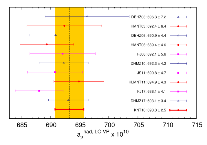
Refer to caption
Figure 24: Comparison of recent and previous evaluations of aμhad,LOVPsuperscriptsubscript𝑎𝜇hadLOVPa_{\mu}^{\rm had,\,LO\,VP} determined from e+ehadronssuperscript𝑒superscript𝑒hadronse^{+}e^{-}\rightarrow{\rm hadrons} cross section data. The analyses listed in chronological order are: DEHZ03 [79], HMNT03 [7], DEHZ06 [80], HMNT06 [8], FJ06 [81], DHMZ10 [82], JS11 [83], HLMNT11 [9], FJ17 [84] and DHMZ17 [78]. The prediction from this work is listed as KNT18, which defines the uncertainty band that the other analyses are compared to.

3.10 SM prediction of g2𝑔2g-2 of the muon

The Standard Model (SM) prediction of the anomalous magnetic moment of the muon is determined by summing the contributions from all sectors of the SM, such that

aμSM=aμQED+aμEW+aμhad,superscriptsubscript𝑎𝜇SMsuperscriptsubscript𝑎𝜇QEDsuperscriptsubscript𝑎𝜇EWsuperscriptsubscript𝑎𝜇hada_{\mu}^{\rm SM}=a_{\mu}^{\rm QED}+a_{\mu}^{\rm EW}+a_{\mu}^{\rm had}\,, (3.31)

where aμQEDsuperscriptsubscript𝑎𝜇QEDa_{\mu}^{\rm QED} is the QED contribution, aμEWsuperscriptsubscript𝑎𝜇EWa_{\mu}^{\rm EW} is the electro-weak contribution and aμhadsuperscriptsubscript𝑎𝜇hada_{\mu}^{\rm had} are the hadronic contributions due to the hadronic vacuum polarisation and hadronic light-by-light scattering (see equation (1.2)). The QED contributions are known up to and including five-loop accuracy. The five-loop calculation has recently been completed numerically by Kinoshita et al. [86, 87] to evaluate all 12,762 five-loop diagrams. This calculation includes all contributions that are due to photons and leptons alone. They are found to be

aμQEDsuperscriptsubscript𝑎𝜇QED\displaystyle a_{\mu}^{\rm QED} =11 658 471.8971(0.0007)(0.0017)(0.0006)(0.0072)×1010absent11658471.89710.00070.00170.00060.0072superscript1010\displaystyle=11\ 658\ 471.8971\ (0.0007)\ (0.0017)\ (0.0006)\ (0.0072)\times 10^{-10}
=(11 658 471.8971±0.007)×1010,absentplus-or-minus11658471.89710.007superscript1010\displaystyle=(11\ 658\ 471.8971\pm 0.007)\times 10^{-10}\,, (3.32)

where the uncertainties are owing to the uncertainty on the lepton masses, the four-loop contributions, the five-loop contributions and the determination of α𝛼\alpha using measurements of Rb87superscriptRb87{}^{87}{\rm Rb}, respectively. With such a precise determination of aμQEDsuperscriptsubscript𝑎𝜇QEDa_{\mu}^{\rm QED} resulting from a perturbative series that converges extremely well, the QED result seems stable. It should be noted, however, that the four-loop and five-loop contributions rely heavily on numerical integrations and independent checks of these results are crucial. This has been recently accomplished through several different analyses [88, 89, 90, 91, 92, 93, 94], which corroborate the results from Kinoshita and collaborators. Therefore, it is safe to assume that the estimate for the QED contribution is well under control.

The contribution from the EW sector is well known to two-loop accuracy [95, 96, 97, 98, 99]. With the mass of the Higgs now known, the updated estimate [100] gives

aμEW=(15.36±0.10)×1010,superscriptsubscript𝑎𝜇EWplus-or-minus15.360.10superscript1010a_{\mu}^{\rm EW}=(15.36\pm 0.10)\times 10^{-10}\,, (3.33)

where the knowledge of the Higgs mass has halved the uncertainty of this contribution compared to the estimate used in [9]. Although a relatively small contribution when compared to aμQEDsuperscriptsubscript𝑎𝜇QEDa_{\mu}^{\rm QED}, the uncertainty is not negligible considering the projected experimental accuracy, but is small when compared to the hadronic uncertainties. However, with this contribution known safely to two-loop accuracy, the electroweak estimate is also very well under control.

For the hadronic vacuum polarisation contributions, the leading order and next-to-leading order contributions have been calculated in this work. The LO contribution, from equation (3.7), was found to be aμhad,LOVP=(693.26±2.46)×1010superscriptsubscript𝑎𝜇hadLOVPplus-or-minus693.262.46superscript1010a_{\mu}^{\rm had,\,LO\,VP}=(693.26\pm 2.46)\times 10^{-10} and the NLO was given in equation (3.7) as aμhad,NLOVP=(9.82±0.04)×1010superscriptsubscript𝑎𝜇hadNLOVPplus-or-minus9.820.04superscript1010a_{\mu}^{\rm had,\,NLO\,VP}=(-9.82\pm 0.04)\times 10^{-10}. The calculation of the NNLO hadronic vacuum polarisation contribution has been achieved for the first time in [13] (see also the evaluation in [84]), where contributions from five individual classes of diagrams (each with an independent, respective kernel function) were determined. It was found to be aμhad,NNLOVP=(1.24±0.01)×1010.superscriptsubscript𝑎𝜇hadNNLOVPplus-or-minus1.240.01superscript1010a_{\mu}^{\rm had,\,NNLO\,VP}=(1.24\pm 0.01)\times 10^{-10}. This estimate is slightly larger than expected and results in a slight increase to the mean value of aμhad,VPsuperscriptsubscript𝑎𝜇hadVPa_{\mu}^{\rm had,VP}. Summing these, the total contribution to the anomalous magnetic moment from the hadronic vacuum polarisation is

aμhad,VP=(684.68±2.42)×1010.superscriptsubscript𝑎𝜇hadVPplus-or-minus684.682.42superscript1010a_{\mu}^{\rm had,\,VP}=(684.68\pm 2.42)\times 10^{-10}\,. (3.34)

It should be noted that the negative NLO contribution results in an anti-correlation between its uncertainty and the uncertainty from the LO contribution, consequently resulting in a slight reduction in the overall uncertainty that has been incorporated into equation (3.34).

The hadronic LbL contributions, although small compared to the hadronic vacuum polarisation sector, have, in the past, been determined through model-dependent approaches. These are based on meson exchanges, the large Ncsubscript𝑁𝑐N_{c} limit, ChPT estimates, short distance constraints from the operator product expansion and pQCD. Over time, several different approaches to evaluating aμhad,LbLsuperscriptsubscript𝑎𝜇hadLbLa_{\mu}^{\rm had,\,LbL} have been attempted, resulting in good agreement for the leading Ncsubscript𝑁𝑐N_{c} (π0superscript𝜋0\pi^{0} exchange) contribution, but differing for sub-leading effects. A commonly quoted determination of the LbL contribution is the ‘Glasgow consensus’ estimate of aμhad,LbL(‘Glasgow consensus’)=(10.5±2.6)×1010superscriptsubscript𝑎𝜇hadLbL‘Glasgow consensus’plus-or-minus10.52.6superscript1010a_{\mu}^{\rm had,\,LbL}(\text{`Glasgow consensus'})=(10.5\pm 2.6)\times 10^{-10} [101] (alternatively, see [102, 103, 104, 105]). However, recent works [106, 107, 108] have re-evaluated the contribution to aμhad,LbLsuperscriptsubscript𝑎𝜇hadLbLa_{\mu}^{\rm had,LbL} due to axial exchanges, where it has been found that this contribution has, in the past, been overestimated due to an incorrect assumption that the form factors for the axial meson contribution are symmetric under the exchange of two photon momenta [106]. Under this assumption, the determination in [102] previously found the axial vector contribution to be aμhad,LbL;axial=(2.2±0.5)×1010superscriptsubscript𝑎𝜇hadLbLaxialplus-or-minus2.20.5superscript1010a_{\mu}^{\rm had,\,LbL;\,axial}=(2.2\pm 0.5)\times 10^{-10}. Correcting this reduces this contribution to aμhad,LbL;axial=(0.8±0.3)×1010superscriptsubscript𝑎𝜇hadLbLaxialplus-or-minus0.80.3superscript1010a_{\mu}^{\rm had,\,LbL;\,axial}=(0.8\pm 0.3)\times 10^{-10} [106, 107]. Applying this adjustment to the ‘Glasgow consensus’ result (which used a value of the axial vector contribution in [101] of aμhad,LbL;axial=(1.5±1.0)×1010superscriptsubscript𝑎𝜇hadLbLaxialplus-or-minus1.51.0superscript1010a_{\mu}^{\rm had,\,LbL;\,axial}=(1.5\pm 1.0)\times 10^{-10}), the estimate in [108] finds

aμhad,LbL=(9.8±2.6)×1010,superscriptsubscript𝑎𝜇hadLbLplus-or-minus9.82.6superscript1010a_{\mu}^{\rm had,\,LbL}=(9.8\pm 2.6)\times 10^{-10}\ \,, (3.35)

which is the chosen estimate for aμhad,LbLsuperscriptsubscript𝑎𝜇hadLbLa_{\mu}^{\rm had,\,LbL} in this work. This result is notably lower than the previously accepted LbL estimates and will incur an overall downward shift on aμSMsuperscriptsubscript𝑎𝜇SMa_{\mu}^{\rm SM}. It is, however, still within the original uncertainties when comparing with the original ‘Glasgow consensus’ estimate. Alternatively, it should be noted that the estimate of aμhad,LbL=(10.2±3.9)×1010superscriptsubscript𝑎𝜇hadLbLplus-or-minus10.23.9superscript1010a_{\mu}^{\rm had,\,LbL}=(10.2\pm 3.9)\times 10^{-10} [108, 109], which is a result that is independent of the ‘Glasgow consensus’ estimate, could be employed here. In addition, the recent work [105] has provided an estimate for the next-to-leading order hadronic LbL contribution. It has found aμhad,NLOLbL=(0.3±0.2)×1010superscriptsubscript𝑎𝜇hadNLOLbLplus-or-minus0.30.2superscript1010a_{\mu}^{\rm had,NLO-LbL}=(0.3\pm 0.2)\times 10^{-10}, which does not alter the hadronic LbL contribution significantly, but is taken into account in the full SM prediction given below.
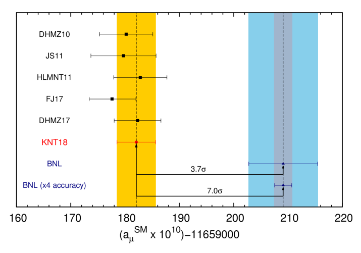
Refer to caption
Figure 25: A comparison of recent and previous evaluations of aμSMsuperscriptsubscript𝑎𝜇SMa_{\mu}^{\rm SM}. The analyses listed in chronological order are: DHMZ10 [82], JS11 [83], HLMNT11 [9], FJ17 [84] and DHMZ17 [78]. The prediction from this work is listed as KNT18, which defines the uncertainty band that other analyses are compared to. The current uncertainty on the experimental measurement [1, 2, 3, 4] is given by the light blue band. The light grey band represents the hypothetical situation of the new experimental measurement at Fermilab yielding the same mean value for aμexpsuperscriptsubscript𝑎𝜇expa_{\mu}^{\rm exp} as the BNL measurement, but achieving the projected four-fold improvement in its uncertainty [5].

Much work has also been directed at the possibility of a model independent calculation of aμhad,LbLsuperscriptsubscript𝑎𝜇hadLbLa_{\mu}^{\rm had,LbL} to further consolidate the SM prediction of aμsubscript𝑎𝜇a_{\mu}. One approach involves the measurement of transition form factors by KLOE-2 and BESIII, which can be expected to constrain the leading pseudoscalar-pole (π0,η,ηsuperscript𝜋0𝜂superscript𝜂\pi^{0},\eta,\eta^{\prime}) contribution to a precision of approximately 15% [108]. Alternatively, the pion transition form factor (π0γγsuperscript𝜋0superscript𝛾superscript𝛾\pi^{0}\rightarrow\gamma^{*}\gamma^{*}) can be calculated on the lattice for the same purpose [110]. New efforts into the prospects of determining aμhad,LbLsuperscriptsubscript𝑎𝜇hadLbLa_{\mu}^{\rm had,LbL} using dispersive approaches are also very promising [111, 112, 113, 114, 115, 116], where the dispersion relations are formulated to calculate either the general hadronic LbL tensor or to calculate aμhad,LbLsuperscriptsubscript𝑎𝜇hadLbLa_{\mu}^{\rm had,LbL} directly. These approaches will allow for the determination of the hadronic LbL contributions from experimental data and, at the very least, will invoke stringent constraints on future estimates. Lastly, there has been huge progress in developing methods for a direct lattice simulation of aμhad,LbLsuperscriptsubscript𝑎𝜇hadLbLa_{\mu}^{\rm had,LbL} [117, 118, 119, 120, 121, 122, 123, 110]. With a proof of principle already well established, an estimate of approximately 10% accuracy seems possible in the near future. Considering these developments and the efforts of the Muon g2𝑔2g-2 Theory Initiative [124] to promote the collaborative work of many different groups, the determination of aμhad,LbLsuperscriptsubscript𝑎𝜇hadLbLa_{\mu}^{\rm had,LbL} on the level of the ‘Glasgow consensus’ will, at the very least, be consolidated and a reduction of the uncertainty seems highly probable on the timescales of the new g2𝑔2g-2 experiments.

Following equation (3.31), the sum of all the sectors of the SM results in a total value of the anomalous magnetic moment of the muon of

aμSM=(11 659 182.04±3.56)×1010,superscriptsubscript𝑎𝜇SMplus-or-minus11659182.043.56superscript1010a_{\mu}^{\rm SM}=(11\ 659\ 182.04\pm 3.56)\times 10^{-10}\,, (3.36)

where the uncertainty is determined from the uncertainties of the individual SM contributions added in quadrature. Comparing this with the current experimental measurement given in equation (1.1) results in a deviation of

Δaμ=(27.06±7.26)×1010,Δsubscript𝑎𝜇plus-or-minus27.067.26superscript1010\displaystyle\Delta a_{\mu}=(27.06\pm 7.26)\times 10^{-10}\,, (3.37)

corresponding to a 3.7σ3.7𝜎3.7\sigma discrepancy. This result is compared with other determinations of aμSMsuperscriptsubscript𝑎𝜇SMa_{\mu}^{\rm SM} in Figure 25. In particular, a comparison with the HLMNT11 estimate given in equation (1.7) shows an improvement in the total uncertainty of aμSMsuperscriptsubscript𝑎𝜇SMa_{\mu}^{\rm SM} of 27%similar-toabsentpercent27\sim 27\%. It should be noted that although, as stated above, the DHMZ17 estimate for aμhad,LOVPsuperscriptsubscript𝑎𝜇hadLOVPa_{\mu}^{\rm had,\,LO\,VP} [78] is lower than the value obtained in this work, the estimate of aμSMsuperscriptsubscript𝑎𝜇SMa_{\mu}^{\rm SM} from DHMZ17 is higher than the estimate from this analysis as DHMZ17 choose to use the estimate for the hadronic light-by-light contribution of aμhad,LbL=(10.5±2.6)×1010superscriptsubscript𝑎𝜇hadLbLplus-or-minus10.52.6superscript1010a_{\mu}^{\rm had,LbL}=(10.5\pm 2.6)\times 10^{-10} [101].

3.11 Determination of α(MZ2)𝛼superscriptsubscript𝑀𝑍2\alpha(M_{Z}^{2})

From equation (3.7), the five-flavour hadronic contribution to Δα(MZ2)Δ𝛼superscriptsubscript𝑀𝑍2\Delta\alpha(M_{Z}^{2}) is found to be Δαhad(5)(MZ2)=(276.11±1.11)×104Δsuperscriptsubscript𝛼had5superscriptsubscript𝑀𝑍2plus-or-minus276.111.11superscript104\Delta\alpha_{\rm had}^{(5)}(M_{Z}^{2})\allowbreak=(276.11\pm 1.11)\times 10^{-4}. Combining this with the leptonic contribution Δαlep(MZ2)=(314.979±0.002)×104Δsubscript𝛼lepsuperscriptsubscript𝑀𝑍2plus-or-minus314.9790.002superscript104\Delta\alpha_{\rm lep}(M_{Z}^{2})=(314.979\pm 0.002)\times 10^{-4} [125, 126] and the contribution due to the top quark Δαtop(MZ2)=(0.7180±0.0054)×104Δsubscript𝛼topsuperscriptsubscript𝑀𝑍2plus-or-minus0.71800.0054superscript104\Delta\alpha_{\rm top}(M_{Z}^{2})=(-0.7180\pm 0.0054)\times 10^{-4} [127, 128], the total value of the QED coupling at the Z boson mass is found in this work to be

α1(MZ2)superscript𝛼1superscriptsubscript𝑀𝑍2\displaystyle\alpha^{-1}(M_{Z}^{2}) =(1Δαlep(MZ2)Δαhad(5)(MZ2)Δαtop(MZ2))α1absent1Δsubscript𝛼lepsuperscriptsubscript𝑀𝑍2Δsuperscriptsubscript𝛼had5superscriptsubscript𝑀𝑍2Δsubscript𝛼topsuperscriptsubscript𝑀𝑍2superscript𝛼1\displaystyle=\Big{(}1-\Delta\alpha_{\rm lep}(M_{Z}^{2})-\Delta\alpha_{\rm had}^{(5)}(M_{Z}^{2})-\Delta\alpha_{\rm top}(M_{Z}^{2})\Big{)}\alpha^{-1}
=128.946±0.015.absentplus-or-minus128.9460.015\displaystyle=128.946\pm 0.015\,. (3.38)

Here, the top contribution is determined using the top quark mass, mt=173.1±0.6subscript𝑚𝑡plus-or-minus173.10.6m_{t}=173.1\pm 0.6 GeV and the value for strong coupling constant at the mass of the Z𝑍Z boson, αs(MZ)=0.1182(12)subscript𝛼𝑠subscript𝑀𝑍0.118212\alpha_{s}(M_{Z})=0.1182(12) [4]. A comparison of these results with other determinations of Δαhad(5)(MZ2)Δsuperscriptsubscript𝛼had5superscriptsubscript𝑀𝑍2\Delta\alpha_{\rm had}^{(5)}(M_{Z}^{2}) and α1(MZ2)superscript𝛼1superscriptsubscript𝑀𝑍2\alpha^{-1}(M_{Z}^{2}) is given in Table 6. Note that, as discussed in Section 3.7, the different weighting of the kernel function of the Δαhad(5)(MZ2)Δsuperscriptsubscript𝛼had5superscriptsubscript𝑀𝑍2\Delta\alpha_{\rm had}^{(5)}(M_{Z}^{2}) dispersion integral compared to the integral for aμhad,LOVPsuperscriptsubscript𝑎𝜇hadLOVPa_{\mu}^{\rm had,\,LO\,VP} results in contributions from higher energy regions having a larger influence on Δαhad(5)(MZ2)Δsuperscriptsubscript𝛼had5superscriptsubscript𝑀𝑍2\Delta\alpha_{\rm had}^{(5)}(M_{Z}^{2}) than on aμhad,LOVPsuperscriptsubscript𝑎𝜇hadLOVPa_{\mu}^{\rm had,\,LO\,VP}. Therefore, the choice to use either the available inclusive data or pQCD above 2similar-toabsent2\sim 2 GeV as discussed in Section 3.9 can have marked differences on the values and errors obtained for Δαhad(5)(MZ2)Δsuperscriptsubscript𝛼had5superscriptsubscript𝑀𝑍2\Delta\alpha_{\rm had}^{(5)}(M_{Z}^{2}).

Analysis Δαhad(5)(MZ2)×104Δsuperscriptsubscript𝛼had5superscriptsubscript𝑀𝑍2superscript104\Delta\alpha_{\rm had}^{(5)}(M_{Z}^{2})\times 10^{4} α1(MZ2)superscript𝛼1superscriptsubscript𝑀𝑍2\alpha^{-1}(M_{Z}^{2})
DHMZ10 [82] 275.59±1.04plus-or-minus275.591.04275.59\pm 1.04 128.952±0.014plus-or-minus128.9520.014128.952\pm 0.014
HLMNT11 [9] 276.26±1.38plus-or-minus276.261.38276.26\pm 1.38 128.944±0.019plus-or-minus128.9440.019128.944\pm 0.019
FJ17 [129] 277.38±1.19plus-or-minus277.381.19277.38\pm 1.19 128.919±0.022plus-or-minus128.9190.022128.919\pm 0.022
DHMZ17 [78] 276.00±0.94plus-or-minus276.000.94276.00\pm 0.94 128.947±0.012plus-or-minus128.9470.012128.947\pm 0.012
KNT18 [This work] 276.11±1.11plus-or-minus276.111.11276.11\pm 1.11 128.946±0.015plus-or-minus128.9460.015128.946\pm 0.015
Table 6: Comparison of recent and previous evaluations of Δαhad(5)(MZ2)Δsuperscriptsubscript𝛼had5superscriptsubscript𝑀𝑍2\Delta\alpha_{\rm had}^{(5)}(M_{Z}^{2}) determined from e+ehadronssuperscript𝑒superscript𝑒hadronse^{+}e^{-}\rightarrow{\rm hadrons} cross section data and the corresponding results for α1(MZ2)superscript𝛼1superscriptsubscript𝑀𝑍2\alpha^{-1}(M_{Z}^{2}).

4 Conclusions and future prospects for the muon g2𝑔2g-2

This analysis, KNT18, has completed a full re-evaluation of the hadronic vacuum polarisation contributions to the anomalous magnetic moment of the muon, aμhad,VPsuperscriptsubscript𝑎𝜇hadVPa_{\mu}^{\rm had,\,VP}, and the hadronic contributions to the effective QED coupling at the Z𝑍Z boson mass, Δαhad(MZ2)Δsubscript𝛼hadsuperscriptsubscript𝑀𝑍2\Delta\alpha_{\rm had}(M_{Z}^{2}). These quantities have been determined using the available e+ehadronssuperscript𝑒superscript𝑒hadronse^{+}e^{-}\rightarrow{\rm hadrons} cross section data as input into corresponding dispersion relations, with an aim to achieve both accurate and reliable results from a predominantly data driven analysis. Since [9], all aspects concerning the radiative corrections of the data and the data combination have been reassessed in this work. Specifically, the data are now combined using an iterative, linear χ2superscript𝜒2\chi^{2}-minimisation developed from a method that has been advocated to be free of bias and that has been studied in detail. Importantly, this data combination method allows for the full use of any available correlated statistical and systematic uncertainties, incorporating experimental covariance matrices in the combination in a bias-free approach. These changes, plus the large quantity of new hadronic cross section data, have resulted in improved estimates for nearly all hadronic channels. This is particularly true for the π+πsuperscript𝜋superscript𝜋\pi^{+}\pi^{-} channel, where the precision of this final state has improved by approximately one third compared to [9], with aμπ+πsuperscriptsubscript𝑎𝜇superscript𝜋superscript𝜋a_{\mu}^{\pi^{+}\pi^{-}} from both analyses in very good agreement. Importantly, the inclusion of recently released neutral data in the KKπ𝐾𝐾𝜋KK\pi and KK2π𝐾𝐾2𝜋KK2\pi channels has removed the need to rely on isospin relations to estimate these final states. In addition, new inclusive hadronic R𝑅R-ratio data from the KEDR collaboration have improved the inclusive data combination. In particular, they have provided the opportunity to reconsider the transition region between the sum of exclusive states and the inclusive data, which has resulted in the transition point being chosen to be at 1.937 GeV in this work, where the different choices for the data input in this point are in agreement within errors. The complete data compilation has yielded the full hadronic R𝑅R-ratio and its covariance matrix in the energy range mπs11.2subscript𝑚𝜋𝑠11.2m_{\pi}\leq\sqrt{s}\leq 11.2 GeV. Using these combined data, for the muon g2𝑔2g-2, this analysis found aμhad,LOVP=(693.26±2.46)×1010superscriptsubscript𝑎𝜇hadLOVPplus-or-minus693.262.46superscript1010a_{\mu}^{\rm had,\,LO\,VP}=(693.26\pm 2.46)\times 10^{-10} and aμhad,NLOVP=(9.82±0.04)×1010superscriptsubscript𝑎𝜇hadNLOVPplus-or-minus9.820.04superscript1010a_{\mu}^{\rm had,\,NLO\,VP}=(-9.82\pm 0.04)\times 10^{-10}. This has resulted in a new estimate for the Standard Model prediction of aμSM=(11 659 182.04±3.56)×1010superscriptsubscript𝑎𝜇SMplus-or-minus11659182.043.56superscript1010a_{\mu}^{\rm SM}=(11\ 659\ 182.04\pm 3.56)\times 10^{-10}, which deviates from the current experimental measurement by 3.7σ3.7𝜎3.7\sigma. For the effective QED coupling, the new estimate in this work of Δαhad(5)(MZ2)=(276.11±1.11)×104Δsuperscriptsubscript𝛼had5superscriptsubscript𝑀𝑍2plus-or-minus276.111.11superscript104\Delta\alpha_{\rm had}^{(5)}(M_{Z}^{2})=(276.11\pm 1.11)\times 10^{-4} yields an updated value for the QED coupling at the Z𝑍Z boson mass of α1(MZ2)=128.946±0.015superscript𝛼1superscriptsubscript𝑀𝑍2plus-or-minus128.9460.015\alpha^{-1}(M_{Z}^{2})=128.946\pm 0.015.

In general, the predictions for aμSMsuperscriptsubscript𝑎𝜇SMa_{\mu}^{\rm SM} have been further scrutinised and are well established. In particular, the improvements in the uncertainty on the level discussed in [130] are on track in preparation for the new experimental results from Fermilab and J-PARC. The efforts of the Muon g2𝑔2g-2 Theory Initiative and the groups involved within it show great progress and promise in improving the estimate of aμSMsuperscriptsubscript𝑎𝜇SMa_{\mu}^{\rm SM} further. Importantly, it should be noted that there is no indication thus far that the SM prediction does not deviate with the current experimental measurement by more than 3σ3𝜎3\sigma. For the hadronic vacuum polarisation contributions, there is scope to further improve the estimates, as new measurements of the π+πsuperscript𝜋superscript𝜋\pi^{+}\pi^{-} cross section are planned to be released in the near future from BaBar, CMD-3, SND and, possibly, BELLE-2. Also, efforts are currently being made to measure new inclusive R𝑅R-ratio data by BESIII and the experiments at Novosibirsk (SND, CMD-3, KEDR). This, in particular, will benefit the evaluation of Δαhad(5)(MZ2)Δsuperscriptsubscript𝛼had5superscriptsubscript𝑀𝑍2\Delta\alpha_{\rm had}^{(5)}(M_{Z}^{2}) which, as discussed in Section 3.11, is more sensitive than aμhad,LOVPsuperscriptsubscript𝑎𝜇hadLOVPa_{\mu}^{\rm had,\,LO\,VP} to the precision of the data from higher energy regions. In addition, lattice determinations of aμhad,VPsuperscriptsubscript𝑎𝜇hadVPa_{\mu}^{\rm had,\,VP} are rapidly improving. Recent work that combines data from lattice QCD with those from experimental R𝑅R-ratio data have already provided extremely accurate results that are in good agreement with the current estimates from the dispersive method [131]. Furthermore, efforts to experimentally measure aμhad,LOVPsuperscriptsubscript𝑎𝜇hadLOVPa_{\mu}^{\rm had,\,LO\,VP} in the space-like region are progressing [132, 133] and would provide an alternative check of the results from the dispersive approach. Should any or all these advances reduce the uncertainty of aμhad,VPsuperscriptsubscript𝑎𝜇hadVPa_{\mu}^{\rm had,\,VP} even further, the improvement of the hadronic light-by-light estimates will become particularly crucial. This is further driven by the fact that the result for aμhad,VPsuperscriptsubscript𝑎𝜇hadVPa_{\mu}^{\rm had,\,VP} determined in this analysis is the first estimate of the hadronic vacuum polarisation contribution that is more precise than the currently quoted uncertainties for aμhad,LbLsuperscriptsubscript𝑎𝜇hadLbLa_{\mu}^{\rm had,\,LbL}. However, given these developments in improving the Standard Model prediction of aμsubscript𝑎𝜇a_{\mu} and the formidable progress made by the new muon g2𝑔2g-2 experiments at Fermilab and J-PARC, the prospects to either establish the existence of new physics contributing to aμsubscript𝑎𝜇a_{\mu}, or to rule out many new physics scenarios, are highly compelling.

Acknowledgements

We would first like to recognise and whole-heartedly thank Alan Martin and Kaoru Hagiwara for their many-year-long collaboration in [7, 8, 9], and also thank Ruofan Liao for his collaboration in [9]. We would like to thank Simon Eidelman, Fedor Ignatov, Andreas Nyffeler and the DHMZ17 group (Michel Davier, Andreas Hoecker, Bogdan Malaescu and Zhiqing Zhang) for numerous useful discussions. We would also like to acknowledge the discussions within the Working Group on Radiative Corrections and MC Generators for Low Energies (Radio MonteCarLow) and The Muon g2𝑔2g-2 Theory Initiative concerning this work. The work of Alex Keshavarzi is supported by STFC under the consolidated grant ST/N504130/1. The work of Daisuke Nomura is supported by JSPS KAKENHI grant numbers JP16K05323 and JP17H01133. The work of Thomas Teubner is supported by STFC under the consolidated grants ST/L000431/1 and ST/P000290/1.

References

  • [1] G. W. Bennett et al. [Muon g-2 Collaboration], Phys. Rev. Lett.  89 (2002) 101804 [Erratum: Phys. Rev. Lett.  89 (2002) 129903].
  • [2] G. W. Bennett et al. [Muon g-2 Collaboration], Phys. Rev. Lett.  92 (2004) 161802.
  • [3] G. W. Bennett et al. [Muon g-2 Collaboration], Phys. Rev. D 73 (2006) 072003.
  • [4] C. Patrignani et al. (Particle Data Group), Chin. Phys. C, 40, 100001 (2016) and 2017 update.
  • [5] J. Grange et al. [Muon g-2 Collaboration], arXiv:1501.06858 [physics.ins-det].
  • [6] T. Mibe [J-PARC g-2 Collaboration], Chin. Phys. C 34 (2010) 745.
  • [7] K. Hagiwara, A. D. Martin, D. Nomura and T. Teubner, Phys. Rev. D 69 (2004) 093003.
  • [8] K. Hagiwara, A. D. Martin, D. Nomura and T. Teubner, Phys. Lett. B 649 (2007) 173.
  • [9] K. Hagiwara, R. Liao, A. D. Martin, D. Nomura and T. Teubner, J. Phys. G 38 (2011) 085003.
  • [10] S. J. Brodsky and E. de Rafael, Phys. Rev.  168 (1968) 1620.
  • [11] B. E. Lautrup and E. de Rafael, Phys. Rev.  174 (1968) 1835.
  • [12] B. Krause, Phys. Lett. B 390 (1997) 392.
  • [13] A. Kurz, T. Liu, P. Marquard and M. Steinhauser, Phys. Lett. B 734 (2014) 144.
  • [14] A. Keshavarzi, D. Nomura and T. Teubner, in preparation.
  • [15] A. Osterheld et al., SLAC-PUB-4160 (1986).
  • [16] C. Edwards et al., SLAC-PUB-5160 (1990).
  • [17] A. Anastasi et al. [KLOE-2 Collaboration], JHEP 1803 (2018) 173.
  • [18] F. Ambrosino et al. [KLOE Collaboration], Phys. Lett. B 670 (2009) 285.
  • [19] F. Ambrosino et al. [KLOE Collaboration], Phys. Lett. B 700 (2011) 102.
  • [20] F. Jegerlehner (2016),
    www-com.physik.hu-berlin.de/similar-to\simfjeger/alphaQED16.tar.gz,
    also see talk by F. Jegerlehner at the Linear Collider Workshop 2010 (http://www-com.physik.hu-berlin.de/similar-to\simfjeger/SMalphas1.pdf).
  • [21] F. Jegerlehner (2003),
    https://www-com.physik.hu-berlin.de/similar-to\simfjeger/alphaQEDn.uu.
  • [22] A. Hoefer, J. Gluza and F. Jegerlehner, Eur. Phys. J. C 24 (2002) 51.
  • [23] J. Gluza, A. Hoefer, S. Jadach and F. Jegerlehner, Eur. Phys. J. C 28 (2003) 261.
  • [24] J. P. Lees et al. [BaBar Collaboration], Phys. Rev. D 92 (2015) 7, 072015.
  • [25] R. R. Akhmetshin et al., Phys. Lett. B 364 (1995) 199.
  • [26] M. N. Achasov et al., Phys. Rev. D 63 (2001) 072002.
  • [27] F. Jegerlehner and K. Kolodziej, Eur. Phys. J. C 77 (2017) 254.
  • [28] K. Kołodziej, Comput. Phys. Commun.  196 (2015) 563.
  • [29] B. Aubert et al. [BaBar Collaboration], Phys. Rev. Lett.  103 (2009) 231801.
  • [30] R. D. Ball et al. [NNPDF Collaboration], JHEP 1005 (2010) 075.
  • [31] M. Benayoun, P. David, L. DelBuono and F. Jegerlehner, Eur. Phys. J. C 75 (2015) 613.
  • [32] G. D’Agostini, Nucl. Instrum. Meth. A 346 (1994) 306.
  • [33] V. Blobel, eConf C 030908 (2003) MOET002.
  • [34] D. Babusci et al. [KLOE Collaboration], Phys. Lett. B 720 (2013) 336.
  • [35] M. Ablikim et al. [BESIII Collaboration], Phys. Lett. B 753 (2016) 629.
  • [36] V. M. Aul’chenko et al., J. Exp. Theor. Phys.  121 (2015), 27.
  • [37] B. Aubert et al. [BaBar Collaboration], Phys. Rev. D 70 (2004) 072004.
  • [38] R. R. Akhmetshin et al., Phys. Lett. B 642 (2006) 203.
  • [39] S. Eidelman and F. Ignatov, private communication (2017).
  • [40] J. P. Lees et al. [BaBar Collaboration], Phys. Rev. D 85 (2012) 112009.
  • [41] B. Aubert et al. [BaBar Collaboration], Phys. Rev. D 71 (2005) 052001.
  • [42] R. R. Akhmetshin et al., Phys. Lett. B 768 (2017) 345.
  • [43] C. Paulot, Doctoral Thesis (1979) Preprint, LAL-79/14.
  • [44] J. P. Lees et al. [BaBar Collaboration], Phys. Rev. D 96 (2017) 092009.
  • [45] J. P. Lees et al. [BaBar Collaboration], Phys. Rev. D 88 (2013) 032013.
  • [46] E. A. Kozyrev et al., Phys. Lett. B 779 (2018) 64.
  • [47] R. R. Akhmetshin et al. [CMD-2 Collaboration], Phys. Lett. B 669 (2008) 217.
  • [48] S. Eidelman, F. Ignatov and E. Kozyrev, private communication (2017).
  • [49] M. N. Achasov et al., Phys. Rev. D 94 (2016) 112006.
  • [50] J. P. Lees et al. [BaBar Collaboration], Phys. Rev. D 89 (2014) 092002.
  • [51] E. A. Kozyrev et al. [CMD-3 Collaboration], Phys. Lett. B 760 (2016) 314.
  • [52] R. R. Akhmetshin et al. [CMD-2 Collaboration], Phys. Lett. B 466 (1999) 385 [Erratum: Phys. Lett. B 508 (2001) 217].
  • [53] J. P. Lees et al. [BaBar Collaboration], Phys. Rev. D 95 (2017) 052001.
  • [54] M. N. Achasov et al., Phys. Rev. D 97 (2018) 032011.
  • [55] J. P. Lees et al. [BaBar Collaboration], Phys. Rev. D 95 (2017) 092005.
  • [56] B. Aubert et al. [BaBar Collaboration], Phys. Rev. Lett.  102 (2009) 012001.
  • [57] R. Liao [HLMNT11], The anomalous magnetic moment of the muon and the QED coupling at the Z boson mass, Doctoral Thesis (2011), University of Liverpool, UK.
  • [58] R. V. Harlander and M. Steinhauser, Comput. Phys. Commun.  153 (2003) 244.
  • [59] R. Ammar et al. [CLEO Collaboration], Phys. Rev. D 57 (1998) 1350.
  • [60] D. Besson et al. [CLEO Collaboration], Phys. Rev. D 76 (2007) 072008.
  • [61] E. Rice et al., Phys. Rev. Lett.  48 (1982) 906.
  • [62] V. V. Anashin et al., Phys. Lett. B 770 (2017) 174.
  • [63] V. V. Anashin et al., Phys. Lett. B 753 (2016) 533.
  • [64] M. Ablikim et al. [BES Collaboration], Phys. Lett. B 677 (2009) 239.
  • [65] M. N. Achasov et al. [SND Collaboration], Phys. Rev. D 93 (2016) 092001.
  • [66] R. R. Akhmetshin et al. [CMD-3 Collaboration], Phys. Lett. B 723 (2013) 82.
  • [67] M. N. Achasov et al., Phys. Rev. D 90 (2014) 032002.
  • [68] M. N. Achasov et al., Phys. Rev. D 97 (2018) 012008.
  • [69] J. P. Lees et al. [BaBar Collaboration], Phys. Rev. D 97 (2018) 052007.
  • [70] R. R. Akhmetshin et al. [CMD-3 Collaboration], Phys. Lett. B 773 (2017) 150.
  • [71] M. N. Achasov et al., Phys. Rev. D 94 (2016) 092002.
  • [72] M. N. Achasov et al., JETP Lett.  94 (2012) 734.
  • [73] M. N. Achasov et al., Phys. Rev. D 94 (2016) 112001.
  • [74] M. N. Achasov et al., Phys. Rev. D 94 (2016) 032010.
  • [75] B. Aubert et al. [BaBar Collaboration], Phys. Rev. D 77 (2008) 092002.
  • [76] R. R. Akhmetshin et al. [CMD-3 Collaboration], Phys. Lett. B 759 (2016) 634.
  • [77] M. N. Achasov et al., Phys. Rev. D 90 (2014) 112007.
  • [78] M. Davier, A. Hoecker, B. Malaescu and Z. Zhang, Eur. Phys. J. C 77 (2017) 827.
  • [79] M. Davier, S. Eidelman, A. Höcker and Z. Zhang, Eur. Phys. J. C 31 (2003) 503.
  • [80] M. Davier, Nucl. Phys. Proc. Suppl.  169 (2007) 288.
  • [81] F. Jegerlehner, Nucl. Phys. Proc. Suppl.  162 (2006) 22.
  • [82] M. Davier, A. Hoecker, B. Malaescu and Z. Zhang, Eur. Phys. J. C 71 (2011) 1515 [Erratum: Eur. Phys. J. C 72 (2012) 1874].
  • [83] F. Jegerlehner and R. Szafron, Eur. Phys. J. C 71 (2011) 1632.
  • [84] F. Jegerlehner, EPJ Web Conf.  166 (2018) 00022.
  • [85] F. Jegerlehner, Springer Tracts Mod. Phys.  274 (2017) 1.
  • [86] T. Aoyama, M. Hayakawa, T. Kinoshita and M. Nio, Phys. Rev. Lett.  109 (2012) 111808.
  • [87] T. Aoyama, T. Kinoshita and M. Nio, Phys. Rev. D 97 (2018) 036001.
  • [88] A. L. Kataev, Phys. Rev. D 86 (2012) 013010.
  • [89] P. A. Baikov, A. Maier and P. Marquard, Nucl. Phys. B 877 (2013) 647.
  • [90] A. Kurz, T. Liu, P. Marquard and M. Steinhauser, Nucl. Phys. B 879 (2014) 1.
  • [91] A. Kurz, T. Liu, P. Marquard, A. V. Smirnov, V. A. Smirnov and M. Steinhauser, Phys. Rev. D 92 (2015) 073019.
  • [92] A. Kurz, T. Liu, P. Marquard, A. Smirnov, V. Smirnov and M. Steinhauser, Phys. Rev. D 93 (2016) 053017.
  • [93] S. Laporta, Phys. Lett. B 772 (2017) 232.
  • [94] S. Volkov, Phys. Rev. D 96 (2017) 096018.
  • [95] A. Czarnecki, B. Krause and W. J. Marciano, Phys. Rev. D 52 (1995) R2619.
  • [96] A. Czarnecki, B. Krause and W. J. Marciano, Phys. Rev. Lett.  76 (1996) 3267.
  • [97] S. Peris, M. Perrottet and E. de Rafael, Phys. Lett. B 355 (1995) 523.
  • [98] A. Czarnecki, W. J. Marciano and A. Vainshtein, Phys. Rev. D 67 (2003) 073006 [Erratum: Phys. Rev. D 73 (2006) 119901].
  • [99] A. Czarnecki and W. J. Marciano, Phys. Rev. D 96 (2017) 113001 [Erratum: Phys. Rev. D 97 (2018) 019901].
  • [100] C. Gnendiger, D. Stöckinger and H. Stöckinger-Kim, Phys. Rev. D 88 (2013) 053005.
  • [101] J. Prades, E. de Rafael and A. Vainshtein, Adv. Ser. Direct. High Energy Phys.  20 (2009) 303.
  • [102] K. Melnikov and A. Vainshtein, Phys. Rev. D 70 (2004) 113006.
  • [103] A. Nyffeler, Phys. Rev. D 79 (2009) 073012.
  • [104] F. Jegerlehner and A. Nyffeler, Phys. Rept.  477 (2009) 1.
  • [105] G. Colangelo, M. Hoferichter, A. Nyffeler, M. Passera and P. Stoffer, Phys. Lett. B 735 (2014) 90.
  • [106] F. Jegerlehner, EPJ Web Conf.  118 (2016) 01016.
  • [107] V. Pauk and M. Vanderhaeghen, Eur. Phys. J. C 74 (2014) 3008.
  • [108] A. Nyffeler, Phys. Rev. D 94 (2016) 053006.
  • [109] A. Nyffeler, arXiv:1710.09742 [hep-ph].
  • [110] A. Gérardin, H. B. Meyer and A. Nyffeler, Phys. Rev. D 94 (2016) 074507.
  • [111] G. Colangelo, M. Hoferichter, M. Procura and P. Stoffer, JHEP 1409 (2014) 091.
  • [112] G. Colangelo, M. Hoferichter, B. Kubis, M. Procura and P. Stoffer, Phys. Lett. B 738 (2014) 6.
  • [113] V. Pauk and M. Vanderhaeghen, Phys. Rev. D 90 (2014) 113012.
  • [114] G. Colangelo, M. Hoferichter, M. Procura and P. Stoffer, JHEP 1509 (2015) 074.
  • [115] G. Colangelo, M. Hoferichter, M. Procura and P. Stoffer, Phys. Rev. Lett.  118 (2017) 232001.
  • [116] G. Colangelo, M. Hoferichter, M. Procura and P. Stoffer, JHEP 1704 (2017) 161.
  • [117] V. Pascalutsa and M. Vanderhaeghen, Phys. Rev. Lett.  105 (2010) 201603.
  • [118] V. Pascalutsa, V. Pauk and M. Vanderhaeghen, Phys. Rev. D 85 (2012) 116001.
  • [119] T. Blum, S. Chowdhury, M. Hayakawa and T. Izubuchi, Phys. Rev. Lett.  114 (2015) 012001.
  • [120] T. Blum, N. Christ, M. Hayakawa, T. Izubuchi, L. Jin and C. Lehner, Phys. Rev. D 93 (2016) 014503.
  • [121] T. Blum, N. Christ, M. Hayakawa, T. Izubuchi, L. Jin, C. Jung and C. Lehner, Phys. Rev. Lett.  118 (2017) 022005.
  • [122] T. Blum, N. Christ, M. Hayakawa, T. Izubuchi, L. Jin, C. Jung and C. Lehner, Phys. Rev. D 96 (2017) 034515.
  • [123] N. Asmussen, A. Gérardin, H. B. Meyer and A. Nyffeler, EPJ Web Conf.  175 (2018) 06023.
  • [124] The Muon g2𝑔2g-2 Theory Initiative, https://indico.fnal.gov/event/13795/.
  • [125] M. Steinhauser, Phys. Lett. B 429 (1998) 158.
  • [126] C. Sturm, Nucl. Phys. B 874 (2013) 698.
  • [127] K. G. Chetyrkin, J. H. Kühn and M. Steinhauser, Phys. Lett. B 371 (1996) 93; Nucl. Phys. B 482 (1996) 213; Nucl. Phys. B 505 (1997) 40.
  • [128] J. H. Kühn and M. Steinhauser, Phys. Lett. B 437 (1998) 425.
  • [129] F. Jegerlehner, arXiv:1711.06089 [hep-ph].
  • [130] T. Blum, A. Denig, I. Logashenko, E. de Rafael, B. Lee Roberts, T. Teubner and G. Venanzoni, arXiv:1311.2198 [hep-ph].
  • [131] T. Blum et al., arXiv:1801.07224 [hep-lat].
  • [132] C. M. Carloni Calame, M. Passera, L. Trentadue and G. Venanzoni, Phys. Lett. B 746 (2015) 325.
  • [133] G. Abbiendi et al., Eur. Phys. J. C 77 (2017) 139.