Comparing an analytical spacetime metric for a merging binary to a fully nonlinear numerical evolution using curvature scalars

Abstract

We introduce a new geometrically invariant prescription for comparing two different spacetimes based on geodesic deviation. We use this method to compare a family of recently introduced analytical spacetime representing inspiraling black-hole binaries to fully nonlinear numerical solutions to the Einstein equations. Our method can be used to improve analytical spacetime models by providing a local measure of the effects that violations of the Einstein equations will have on timelike geodesics, and indirectly, gas dynamics. We also discuss the advantages and limitations of this method.

I Introduction

Ever since the breakthroughs in numerical relativity in the early 2000s Pretorius (2005); Campanelli et al. (2006); Baker et al. (2006), it has been possible to simulate black-hole binaries (BHBs) for from the rapid inspiral phase, through the plunge and merger. Modern numerical relativity codes are now capable of simulating inspiraling BHBs for over 100 orbits Szilagyi et al. (2015). These simulations are the most accurate known means of generating the gravitational waveform from such mergers. However, they are also computationally expensive. Recently, a family of analytic metric representing the inspiral phase of a BHB was proposed and used extensively to study accretion physics Noble et al. (2012); Gallouin et al. (2012); Mundim et al. (2014); Zilhao et al. (2015); Zlochower et al. (2016); Ireland et al. (2016); Nakano et al. (2016); Bowen et al. (2017a, b).

In this paper, we introduce a new technique to study the accuracy of this family BHB spacetimes by comparing them to full numerical evolutions starting from a set of fiducial separations. Our method is based on analyzing a set of scalars related to geodesic deviation. This study complements previous studies in Ref. Zilhao et al. (2015), where the hydrodynamics and magnetohydrodynamics of accreting gas were compared between versions of the analytical spacetime at different approximation orders.

In this paper, we express tensors in both the more conventional coordinate basis and in orthonormal bases. Latin indices near the beginning of the alphabet are abstract tensor indices Wald (1984), which indicate the type of tensors involved in a calculation, as well as contraction. Latin indices near the end of the alphabet denote coordinate-basis components of spatial tensors, while Greek letters denote 4-dimensional spacetime components in the coordinate basis. Components of tensors in an orthonormal basis (the first element of the orthonormal basis is always timelike) are denoted by a Greek or Latin letter surrounded by square braces. Whether associated with coordinate bases or orthonormal bases, Greek indices range from $0$ to $3$, while Latin indices near the end of the alphabet range from $1$ to $3$. In this paper, we use the geometric unit system, where $G=c=1$.

This paper is organized as follows. In Sec. II, we describe the analytical and numerical techniques used in this paper. In Sec. III, we present the tests we used to confirm the accuracy of our results. In Sec. IV, we describe the results of our study. In Sec. V we discuss the consequences and limitations of our study.

II Techniques

II.1 Analytic Black-Hole Binary Spacetime

In this paper, the analytic metric we consider represents a nonspinning, equal-mass BHB in a quasicircular inspiral. This spacetime was first constructed in Ref. Mundim et al. (2014) based on earlier work on binary initial data in Refs. Yunes et al. (2006); Yunes and Tichy (2006); Johnson-McDaniel et al. (2009).

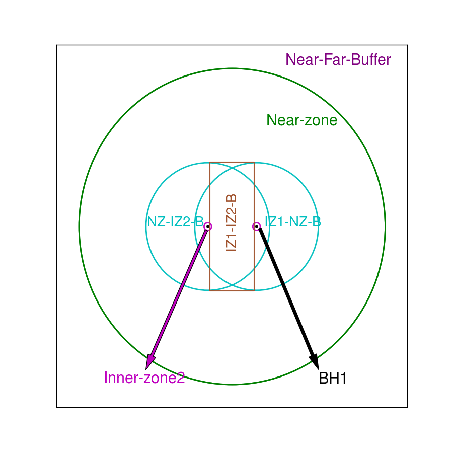
The analytic spacetime is constructed by asymptotically matching metrics in three different zones characterizing three different spacetime regions of validity for different analytic metrics: (i) a far zone (FZ) where the spacetime can be described by a two-body perturbed flat spacetime with outgoing gravitational radiation and where retardation effects are fully accounted for; (ii) a near zone (NZ) which is less than one GW length from the center of mass of the binary [but not too close to each black hole (BH)] that is described by a post-Newtonian metric (this includes retardation effects at a perturbative level and binding interactions between the two BHs); and (iii) inner zones (IZs) that are described by perturbed Schwarzschild (or Kerr) BHs. The full spacetime is then constructed by smoothly transitioning from zone to zone in the so-called buffer zones (BZs).

Figure 1 shows where these regions are located with respect to the two BHs.

Figure 1: The zones for the analytic metric. The large (green) circle is the outer boundary of the near zone. Immediately inside this circle the metric is exclusively the post-Newtonian near-zone metric, while outside, it is a superposition of the near and far zone metrics. All points in the figure outside this circle are in the near-far buffer zone (the other boundary of this zone is not show). The smaller (cyan) circles denote the inner boundary of the near zone. Inside the envelope of these circles is the near-inner buffer zones. The box (orange) denotes the region inside the near-inner buffer zone where the metric is a superposition of both BH1 and BH2 inner zones, as well as the near zone. Outside the box, the metric is a superposition of the near zone metric and either one of the inner zone metrics. Finally inside the very small (magenta) circles are the two inner zones, where the metric is purely the inner zone perturbed Schwarzschild metric.

II.2 Geodesic Analysis

The primary analysis in this paper concerns how the fully nonlinear evolution of initial data based on the analytic metric differs from the analytic metric itself at some later time. In order to do this, we need gauge invariant measurements that can elucidate to what degree two spacetimes are locally similar.

To be precise, on some fiducial spatial slice $\Sigma_{0}$, which corresponds to a surface of constant coordinate time $t=t_{0}$, the induced metric and extrinsic curvatures of the analytic metric are used as initial data for a CCZ4 evolution. Critical to our analysis, on $\Sigma_{0}$, the analytic and numerically evolved metrics are identical. Furthermore, if the analytic metric solved the vacuum Einstein equations, up to truncation error, the numerical and analytic metrics would only differ by a gauge transformation at all later times (at least in the domain of dependence on the initial numerical slice, which will be of finite extent).

The fact that gauges are identical on $\Sigma_{0}$ allows us to use geodesic dynamics to explore how the numerical and analytic spacetimes begin to differ with time. In particular, if we take as initial data for a timelike geodesic some given coordinate position and the spatial projection of the 4-velocity, $V^{a}$ (from which we can reconstruct the full 4-velocity $u^{a}$ at $t_{0}$ via $u^{a}=\sqrt{1+\gamma_{ij}V^{i}V^{j}}n^{a}+V^{a}$, where $V^{0}=0$ and $n^{a}$ is the unit norm to $\Sigma_{0}$), and if the analytic metric solved the vacuum Einstein equations, the resulting geodesic, as calculated on the two metrics, would be geometrically identical. By this, we mean that the two geodesics would only differ by a gauge transformation. The question remains though, how do we show that geodesics in two different gauges are identical or not if the gauge transformation is unknown?

To address this question, we consider measuring curvature scalars along each geodesic as a function of proper time. Our construction of these scalars is as follows.

Let $u^{a}(\tau)$ be the 4-velocity associated with a geodesic (and hence unit norm). At each point along the geodesic construct an orthonormal basis $\{e^{a}_{[0]},\,e^{a}_{[1]},\,e^{a}_{[2]},\,e^{a}_{[3]}\}$, where $e^{a}_{[0]}=u^{a}(\tau)$ and $e^{a}_{[\mu]}e^{b}_{[\nu]}g_{ab}=\eta_{[\mu][\nu]}$. The choice of components 1, 2, and 3 of this basis is arbitrary. Given any such basis, we can define a $3\times 3$ symmetric matrix of scalars ${\bf M}$, where

$${\bf M}=\left(\begin{array}[]{ccc}M_{[1][1]}&M_{[1][2]}&M_{[1][3]}\\ M_{[2][1]}&M_{[2][2]}&M_{[2][3]}\\ M_{[3][1]}&M_{[3][2]}&M_{[3][3]}\\ \end{array}\right)\,,$$ (4)

and

$$M_{[i][j]}=R_{abcd}u^{a}e^{b}_{[i]}u^{c}e^{d}_{[j]},\quad i,j=1,2,3\,.$$ (5)

Importantly, the eigenvalues of this matrix are independent of how $e^{a}_{[1]}$, $e^{a}_{[2]}$, and $e^{a}_{[3]}$ are constructed. This follows because any two choices $(e^{a}_{[1]},\,e^{a}_{[2]},\,e^{a}_{[3]})$ only differ by an orthogonal transformation (which preserves eigenvalues). Consequently, if the analytic metric and numerically evolved metric represented the same spacetime, the eigenvalues of ${\bf M}$ constructed this way on each metric would be identical. We will refer to these eigenvalues as curvature eigenvalues in the sections below.

Of course, the analytic metric, being an approximate solution, violates the vacuum field equations to some degree (see Refs. Mundim et al. (2014); Zilhao et al. (2015) for a detailed analysis). Thus the analytic metric and its numerical evolution will differ to some level. Our goal here is to demonstrate a local measure of how the two spacetimes actually differ. To do this, we note that the elements of $M_{[i][j]}$ have the interpretation of being the (negative of the) acceleration of deviation vector $e^{a}_{[i]}$ along the direction $e^{b}_{[j]}$. We can thus interpret relative differences in the curvature eigenvalues of ${\bf M}$ as proxies for the relative differences in the effective potentials experienced by timelike geodesics traversing these two spacetimes.

One important limitation of our procedure is that because slightly different geodesics can, in principle, follow very different trajectories on secular timescales, our analysis will need to be done at when the geodesics are relatively close to $\Sigma_{0}$. Otherwise, a small difference in the two spacetimes may incorrectly be interpreted as a large difference. We ameliorate this problem by only choosing geodesics that are stable. By this, we mean that the trajectories are largely insensitive to small perturbations of the initial velocity. As such, we do not include cases where small perturbations lead to the geodesic orbiting a different black hole, or ones where small perturbations lead to geodesics falling into either black hole.

We also note that our analysis here can be extended in a straightforward manner to include all 20 independent components of the Riemann tensor. To do this, we would need the vectors $e^{a}_{[i]}$ ($i=1,\,2,\,3$) to obey $u^{b}\nabla_{b}e^{a}_{[i]}=0$. That is, evolve the entire basis. Under this extended construction, all components of

$$R_{[\mu][\nu][\rho][\sigma]}=R_{abcd}e^{a}_{[\mu]}e^{b}_{[\nu]}e^{c}_{[\rho]}e^{d}_{[\sigma]}$$ (6)

are gauge invariant. We can thus compare each component as constructed on the analytic and numerical spacetimes. We leave this analysis for a later work.

II.3 Reconstructing the 4-dimensional Riemann tensor

As is done by in many numerical relativity codes, our numerical evolutions uses the standard 3+1 Arnowitt-Deser-Misner Arnowitt et al. (2008) split of the Einstein equations. In this paper, we will need to reconstruct the full 4-dimensional Riemann tensor from the three dimensional quantities evolved by our code. In this section, we provide the details of how this is accomplished. In order to avoid confusion, we will use the notation $(3)$ and $(4)$ to indicate a three or four dimensional tensors, respectively.

In the standard 3+1 split, the metric on a spatial slice (given by $t={\rm const}$) is obtained from the full 4-dimensional metric via

$$\gamma_{\mu\nu}=g_{\mu\nu}+n_{\mu}n_{\nu}\,,$$ (7)

where $n^{\mu}$ is the unit norm to the spatial hypersurface and the spatial components of this tensor (i.e., indices 1 through 3) form the 3-dimensional metric tensor. Note that while $\gamma_{ij}=g_{ij}$, $\gamma^{ij}\neq g^{ij}$. The full 4-dimensional tensor $\gamma_{\mu\nu}$ also serves as a projection operator which takes four-dimensional tensors to three-dimensional ones. To avoid confusion, we will use $P_{\mu\nu}=\gamma_{\mu\nu}$ to denote the projection tensor.

In order to reconstruct the 4-dimensional Riemann tensor, ${}^{(4)}R_{\mu\nu\epsilon\delta}$, we follow Ref. Baumgarte and Shapiro (2010) and write it as

$${}^{(4)}R_{\mu\nu\epsilon\delta} = P_{\mu}{}^{\zeta}P_{\nu}{}^{\tau}P_{\epsilon}{}^{\kappa}P_{\delta}{}^{\sigma}\ {}^{(4)}R_{\zeta\tau\kappa\sigma}$$ (12)

$$-2P_{\mu}{}^{\zeta}P_{\nu}{}^{\tau}P_{[\epsilon}{}^{\kappa}n_{\delta]}n^{\sigma}\ {}^{(4)}R_{\zeta\tau\kappa\sigma}$$

$$-2P_{\epsilon}{}^{\zeta}P_{\delta}{}^{\tau}P_{[\mu}{}^{\kappa}n_{\nu]}n^{\sigma}\ {}^{(4)}R_{\zeta\tau\kappa\sigma}$$

$$+2P_{\mu}{}^{\zeta}P_{[\epsilon}{}^{\kappa}n_{\delta]}n_{\nu}n^{\tau}n^{\sigma}\ {}^{(4)}R_{\zeta\tau\kappa\sigma}$$

$$-2P_{\nu}{}^{\zeta}P_{[\epsilon}{}^{\kappa}n_{\delta]}n_{\mu}n^{\tau}n^{\sigma}\ {}^{(4)}R_{\zeta\tau\kappa\sigma}\,,$$

where

$$P^{\zeta}{}_{\mu}P^{\eta}{}_{\nu}P^{\kappa}{}_{\epsilon}P^{\sigma}{}_{\delta}\ {}^{(4)}R_{\zeta\eta\kappa\sigma} = {}^{(3)}\!R_{\mu\nu\epsilon\delta}$$ (13)

$$+K_{\mu\epsilon}K_{\nu\delta}-K_{\mu\delta}K_{\epsilon\nu}\,,$$

$$P^{\sigma}{}_{\mu}P^{\eta}{}_{\nu}P^{\kappa}{}_{\delta}n^{\zeta}R_{\sigma\eta\kappa\zeta} = D_{\nu}K_{\mu\delta}-D_{\mu}K_{\nu\delta}\,,$$ (14)

$$P^{\zeta}{}_{\mu}P^{\kappa}{}_{\nu}n^{\delta}n^{\epsilon}R_{\delta\kappa\epsilon\zeta} = \mathcal{L}_{n}K_{\mu\nu}+\frac{1}{\alpha}D_{\mu}D_{\nu}\alpha$$ (15)

$$+K^{\epsilon}{}_{\nu}K_{\mu\epsilon}\,,$$

and $D_{i}$ is the covariant derivative associated with $\gamma_{ij}$, $\alpha$ is the lapse, and $K_{ij}$ is the extrinsic curvature.

Note that the left-hand sides of Eqs. (13)–(15) are all naturally defined in terms of 3-dimensional tensors. To construct a 4-dimension tensor from a 3-dimension tensor $T^{i_{1}i_{2}\cdots}_{j_{1}j_{2}\cdots}$, we use the following operator,

$$T^{\mu_{1}\mu_{2}\cdots}_{\nu_{1}\nu_{2}\cdots}={\Lambda^{\mu_{1}}}_{i_{1}}{\Lambda^{\mu_{2}}}_{i_{2}}\cdots{\Lambda_{\nu_{1}}}^{j_{1}}{\Lambda_{\nu_{2}}}^{j_{2}}\cdots T^{i_{1}i_{2}\cdots}_{j_{1}j_{2}\cdots}\,,$$ (16)

where

$${\Lambda_{\mu}}^{i}=\left(\begin{array}[]{ccc }\beta^{1}&\beta^{2}&\beta^{3}\\ 1&0&0\\ 0&1&0\\ 0&0&1\end{array}\right)\,,$$ (17)

where $\beta^{i}$ is the shift, and

$${\Lambda^{\mu}}_{i}=\left(\begin{array}[]{ccc }0&0&0\\ 1&0&0\\ 0&1&0\\ 0&0&1\end{array}\right)\,.$$ (18)

Finally, the left-hand side of Eq. (15) is evaluated by assuming the standard ADM vacuum evolution equations are obeyed. That is,

$$\mathcal{L}_{n}K_{\mu\nu} = \frac{1}{\alpha}(\mathcal{L}_{t}K_{\mu\nu}-\mathcal{L}_{\beta}K_{\mu\nu})\,,$$ (19)

$$\mathcal{L}_{t}K_{\mu\nu} = -D_{\mu}D_{\nu}\alpha+\alpha({}^{(3)}\!R_{\mu\nu}-2K^{\kappa}{}_{\nu}K_{\mu\kappa}+KK_{\mu\nu})$$ (21)

$$-8\pi\alpha({S_{\mu\nu}-\frac{1}{2}\gamma_{\mu\nu}(S-\rho))}+\mathcal{L}_{\beta}K_{\mu\nu}\,,$$

where $S_{\mu\nu}=\gamma_{\mu}{}^{\kappa}\gamma_{\nu}{}^{\sigma}T_{\kappa\sigma}$, $S=S^{\mu}{}_{\mu}$, and $\rho=n^{\mu}n^{\nu}T_{\mu\nu}$ are all assumed to be zero.

Since we actually evolve the metric using the CCZ4 system Alic et al. (2012), the actual form of the evolution equation for the extrinsic curvature is

$$\mathcal{L}_{t}K_{\mu\nu} = -D_{\mu}D_{\nu}\alpha+\alpha({}^{(3)}\!R_{\mu\nu}-2K^{\kappa}{}_{\nu}K_{\mu\kappa}+KK_{\mu\nu})$$ (25)

$$+\alpha(D_{\mu}Z_{\nu}+D_{\nu}Z_{\mu})$$

$$-\left(2\alpha K_{\mu\nu}+\alpha\gamma_{\mu\nu}\frac{1}{\phi^{2}}\kappa_{1}(1+\kappa_{2})\right)\Theta$$

$$+\mathcal{L}_{\beta}K_{\mu\nu}\,,$$

where $\Theta$ and $Z_{i}$ denote deviations from the Einstein equations, and constants $\kappa_{i}$ are free parameters. Thus using Eq. (21) is equivalent to assuming $\Theta$ and $Z_{i}$ are zero. At $t=0$ this is the case, and both variables remain small due to the constraint damping of the CCZ4 system. In order to make our code more general, we assume Eq. (21), which means that it can be used equally well with a BSSN, CCZ4, or other 3+1 evolution system.

To reconstruct ${}^{(4)}R_{\mu\nu\kappa\sigma}$, we interpolate $\gamma_{ij}$, $\partial_{k}\gamma_{ij}$, the 3-dimensional Ricci tensor ${}^{(3)}R_{ij}$, $K_{ij}$, $\partial_{k}K_{ij}$, $\alpha$, $\beta^{i}$, and $\partial_{j}\beta^{i}$ along each geodesic. Note that we do not need second derivatives of the lapse because the $D_{\mu}D_{\nu}\alpha$ cancel out. From these quantities, we can reconstruct all terms in Eqs. (13)–(15). Note that the 3-dimensional Riemann tensor can be reconstructed directly from the 3-dimensional Ricci tensor.

To compute the Riemann tensor for the analytic spacetime, we use an eighth-order finite differencing algorithm and directly differentiate the 4-dimensional metric.

II.4 Numerical Evolutions

We first explored evolving the analytic metric using the fully nonlinear numerical relativity codes in Ref. Zlochower et al. (2016). We use an identical procedure here, which we summarize below.

We evolved the BHB initial data using the LazEv Zlochower et al. (2005) implementation of the moving puncture approach Campanelli et al. (2006); Baker et al. (2006) with the conformal function $W=\sqrt{\chi}=\exp(-2\phi)$ suggested by Ref. Marronetti et al. (2008) and the Z4 Bona et al. (2003); Bernuzzi and Hilditch (2010); Alic et al. (2012) and BSSN Nakamura et al. (1987); Shibata and Nakamura (1995); Baumgarte and Shapiro (1998) evolution systems. Here, we use the conformal covariant Z4 (CCZ4) implementation of Ref. Alic et al. (2012). Note that the same technique has been recently applied to the evolution of binary neutron stars Kastaun et al. (2013); Alic et al. (2013). For the CCZ4 system, we again used the conformal factor $W$. We used centered eighth-order finite differencing for all spatial derivatives, a fourth-order Runge-Kutta time integrator, and both fifth- and seventh-order Kreiss-Oliger dissipation Kreiss and Oliger (1973).

Our code uses the EinsteinToolkit Löffler et al. (2012); Mösta et al. (2014); ein / Cactus cac / Carpet Schnetter et al. (2004); car infrastructure. The Carpet mesh refinement driver provides a “moving boxes” style of adaptive mesh refinement (AMR). In this approach, refined grids of fixed size are arranged about the coordinate centers of both holes. The Carpet code then moves these fine grids about the computational domain by following the trajectories of the two BHs.

To obtain initial data, we use eighth-order finite differencing of the analytic global metric to obtain the 4-metric and all its first derivatives at every point on our simulation grid. The finite differencing of the global metric is constructed so that the truncation error is negligible compared to the subsequent truncation errors in the full numerical simulation (here we used finite difference step size of $10^{-4}$, which is 90 times smaller than our smallest grid size in any of the numerical simulations discussed below). We then reconstruct the spatial 3-metric $\gamma_{ij}$ and extrinsic curvature $K_{ij}$ from the global metric data. Note that with the exception of the calculation of the extrinsic curvature, we do not use the global metric’s lapse and shift. In order to evolve these data, we need to remove the singularity at the two BH centers. Unlike in the puncture formalism Brandt and Brügmann (1997), the singularities here are true curvature singularities. We stuff Etienne et al. (2007); Brown et al. (2007, 2009) the BH interiors in order to remove the singularity. Our procedure is to replace the singular metric well inside the horizons with nonsingular (but constraint violating) data through the transformations,

$$\gamma_{ij}\to f(r)\ \gamma_{ij}\,,\quad i\neq j\,,$$ (26)

$$\gamma_{ii}\to f(r)\ \gamma_{ii}+(1-f(r))\Xi\,,$$ (27)

$$K_{ij}\to f(r)\ K_{ij}\,,$$ (28)

where

$$f(r)=\left\{\begin{array}[]{lr}0\,,&r<r_{\rm min}\\ 1\,,&r>r_{\rm max}\\ P(r)\,,&r_{\rm min}\leq r\leq r_{\rm max}\end{array}\right.\,.$$ (29)

Here, $r$ is the distance to a BH center, and $P(r)$ is a fifth-order polynomial that obeys $P(r_{\rm min})=P^{\prime}(r_{\rm min})=P^{\prime\prime}(r_{\rm min})=0$, $P(r_{\rm max})=1$, $P^{\prime}(r_{\rm max})=P^{\prime\prime}(r_{\rm max})=0$, and $\Xi$ is a large number. The resulting data are therefore $C^{2}$ globally. The parameters $r_{\rm min}$, $r_{\rm max}$, and $\Xi$ are chosen such that both transitions occur inside the BHs and so that $W$ varies smoothly with negligible shoulders in the transition region and is small at the centers.

The grid structure for the runs below consisted of a course grid extending to $(x,\,y,\,z)=\pm(3200,\,3200,\,3200)M$ (we exploited both the $z$-reflection and $\pi$-rotational symmetry of the data in order to reduce the computational volume by a factor of 4. We used 12 levels of mesh refinement. In the sections below, we indicate the global resolution of each simulation by indicating the number of points on the coarsest grid from the origin to each outer face. That is, a resolution of $N=100$ indicated that the coarsest grid spacing is $3200M/100=32M$. The resolution was always set to be the same in each direction.

To evolve timelike geodesics in the numerical spacetime, we use the following algorithm. The 4-velocity of each geodesic is decomposed into a component tangent to the unit norm $n^{a}$ and a spatial component $V^{a}$. That is,

$$u^{\mu}=\varpi n^{\mu}+V^{\mu}\,,$$ (30)

where $\varpi=\sqrt{1+V^{i}V^{j}\gamma_{ij}}$ and $V^{0}=0$ Hughes et al. (1994) (note that $V_{i}=u_{i}$ $[i=1,2,3]$). The geodesic equation then gives

$$\frac{dx^{i}}{dt} = -\beta^{i}+\frac{\alpha}{\varpi}\,V^{i}\,,$$

$$\frac{d\tau}{dt} = \frac{\alpha}{\varpi}\,,$$

$$\frac{dV_{i}}{dt} = -\varpi\alpha_{,i}-V_{j}{\beta^{j}}_{,i}+\frac{1}{2}V^{j}V^{k}{\gamma_{jk}}_{,i}\,.$$ (31)

This form of the geodesic equation has the advantage that explicit time derivatives of the 4-metric are not needed for the evolution and the integration variable is $t$, which is the time coordinate used in the code. We evolve the geodesics using the same RK4 time integrator used to evolve the metric itself.

Since we evolve these geodesics with an adaptive-mesh code, there are complication associated with geodesics crossing refinement level boundaries. Our algorithm is as follows. The AMR grid is distributed such that on a given refinement level, a single CPU will only own a single Cartesian box. We then search for the finest resolution box that contains that geodesic and assign the evolution of the geodesics (at that time step) to that processor. For our purposes, a geodesic is only contained in a given box if all points used by the interpolation stencil are in that box (excluding buffer zones, but including ghost zones). If a geodesic is too close to buffer zones, then it will be evolved using the next coarsest level.

A geodesic that crosses from a coarse refinement level to a finer one may actually be ahead, in time, of the rest of the fields on that refinement level. In such a case, the evolution of the geodesic is stalled until the time associated with that refinement level catches up. On the other hand, when a geodesic moves from a finer level to a coarser one, it is generally behind. In that case, we use a second-order accurate algorithm to evolve the geodesic forward in time until it is caught up with the rest of the fields on that refinement level.

On the other hand, for the analytic metric, we use the more conventional formulation of the geodesic equation,

$$\frac{dx^{\mu}}{d\tau} = u^{\mu}\,,$$ (32)

$$\frac{du^{\mu}}{d\tau} = -{\Gamma^{\mu}}_{\rho\sigma}u^{\rho}u^{\sigma}\,,$$ (33)

where ${\Gamma^{\mu}}_{\rho\sigma}$ is the 4-dimensional Christoffel symbols. Here, we evolve the geodesics using an adaptive RK45 algorithm.

III Code verification

Our code suite consists of three parts. A stand-alone code written in C++ that integrates geodesics and calculates the Riemann tensor given a function that can provide $g_{\mu\nu}$ at arbitrary coordinate positions. A Cactus Thorn that evolves geodesics alongside the metric within the Einstein Toolkit, as well as interpolates the metric (and derivatives) along these geodesics. Finally, our toolkit contains a set of Python scripts that calculates the curvature eigenvalues of Eq. (4) given the data provided by the previous two programs.

We performed several verification tests of the this code suite, which we will describe here. Our first test consisted of using the stand-alone C++ code to evolve identical geodesics on Schwarzschild backgrounds, but in very different gauges.

To do this, we started with the standard Schwarzschild metric,

$$ds^{2} = -\left(1-\frac{2M}{R}\right)dT^{2}+\left(1-\frac{2M}{R}\right)^{-1}dR^{2}$$ (35)

$$+R^{2}\,d\Theta^{2}+R^{2}\,\sin^{2}\Theta\,d\Phi^{2}\,,$$

and used the simple coordinate transformation,

$$T = t+A\,\sin(\omega t)\,\sin(\omega t)\,\cos(r)\,,$$ (36)

$$R = r+A\,\sin(\omega t)\,\sin(\omega t)\,,$$ (37)

$$\Theta = \theta\,,$$ (38)

$$\Phi = \phi\,,$$ (39)

where $A$ is a constant.

Figure 2: Circular geodesics in standard Schwarzschild and transformed Schwarzschild coordinates. While the trajectory is gauge dependent (top), the associated curvature eigenvalues (only one shown) are not (bottom). The differences between the eigenvalues (Sc) calculated in to the two gauges are consistent with roundoff errors.

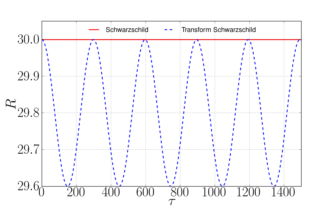
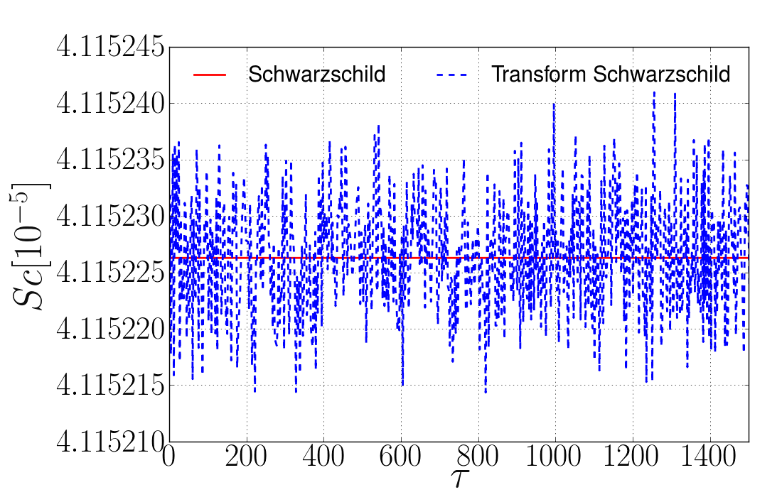
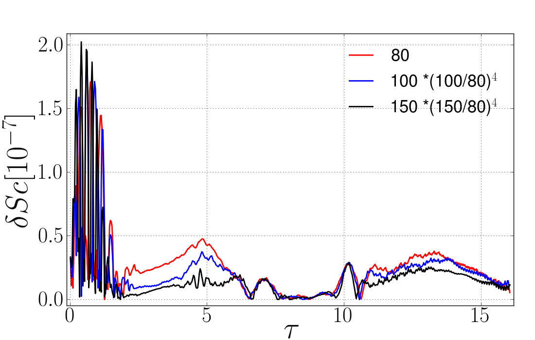
As is readily apparent in Fig. 2, the coordinate trajectory of the geodesic is quite different in the two coordinate systems. However, the calculated curvature eigenvalues (only one shown) are identical. There are three curvature eigenvalues, two are positive with very similar magnitudes and one has a negative value, but is roughly a factor of two larger in absolution value than the other two. When plotting the eigenvalues, we make the fiducial choice of plotting the intermediate eigenvalue, which we denote by Sc in the figures below.

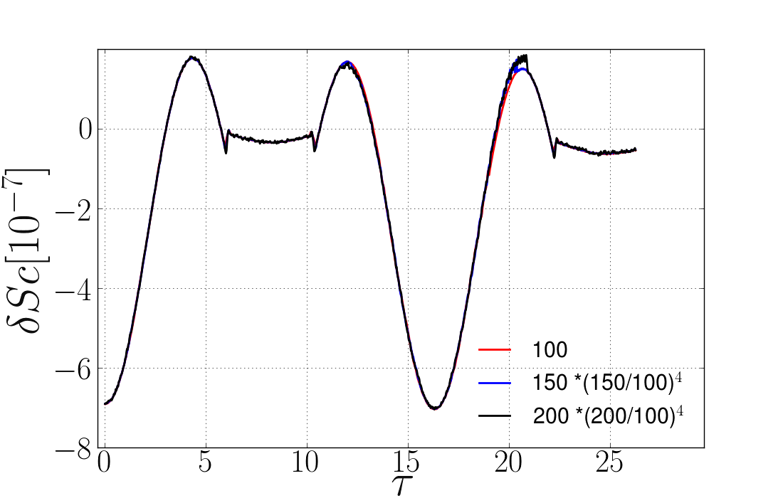
Next, we repeated the same calculation using our EinsteinToolkit-based geodesic thorn. Here we set the metric analytically, but evolved the geodesics, and calculated the Riemann tensor (see Sec. II) numerically. Here, three grid resolutions were used to test the numerical convergence. As shown in Fig. 3, the relative differences between the analytical and numerical evolution of the curvature eigenvalues shows the expected fourth-order convergence.

Figure 3: The differences between one of curvature eigenvalues(Sc) versus time from our new geodesic thorn and the exact values (as determined by a stand-alone code). Here, we denote the resolution of a given simulation by the number of gridpoint, per dimension, from the origin to the outer boundary, and rescale the differences by the ratio of the grid resolution to the fourth power.

To test for convergence of our geodesic thorn in the context of a fully nonlinear numerical spacetime, we evolve the Schwarzschild metric in trumpet coordinates Dennison et al. (2014) (with the trumpet parameter $R_{0}=M$). For reference, the metric has the form,

$$ds^{2}=-\left(\frac{R-M}{R+M}\right)dT^{2}+\frac{2M}{R}dTdR$$ (40)

$$+\left(1+\frac{M}{R}\right)^{2}\left(dR^{2}+R^{2}\,d\Theta^{2}+R^{2}\,\sin^{2}\Theta\,d\Phi^{2}\right)\,.$$ (41)

Following Ref. Dennison and Baumgarte (2014), we use the lapse condition $\partial_{t}\alpha={\cal L}_{\beta}\alpha-\alpha(1-\alpha)K$, for which all the metric functions are constants (up to truncation error) as functions of time.

A convergence plot of the curvature eigenvalues from a fiducial geodesic is shown in Fig. 4. Here, too, we find fourth-order convergence.

Figure 4: The difference between one of the gauge independent curvature eigenvalue (Sc) as calculated using a fully nonlinear numerical evolution of time independent trumpet Schwarzschild data using the EinsteinToolkit, and as calculated using the exact trumpet Schwarzschild metric with the trumpet parameter $R_{0}=M$. Here, we rescale the differences by the ratio of the grid resolution to the fourth power.

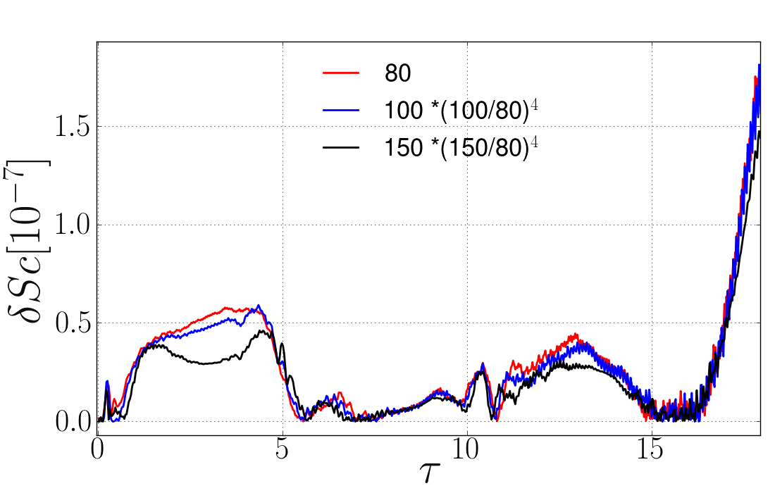
One aspect of numerical evolutions of a binary spacetime on AMR grids that we will encounter is stochastic noise in the curvature Zlochower et al. (2012) due to unresolved gauge waves Etienne et al. (2014). In order to test our code with a time dependent metric, we evolved the same trumpet data, but with a modified lapse condition $\partial_{t}\alpha={\cal L}_{\beta}\alpha-1.001\alpha(1-\alpha)K$. This introduces a small time dependence to the metric without simultaneously introducing an unresolved gauge wave. As seen in Fig. 5, the convergence is still fourth-order. However, when using a more standard puncture-based initial data and $1+\log$ lapse, the convergence order reduced to second-order, which is consistent with the second-order time prolongation we use. The reason for this drop in convergence rate is likely the very rapid evolution of the gauge during the first few $M$ of evolution. These rapid changes can lead to the second order (in time) prolongation error dominating the error budget.

Figure 5: The convergence of the one of the gauge independent curvature eigenvalues (Sc) for a slowly time-dependent Schwarzschild trumpet. The convergence order is still fourth-order.

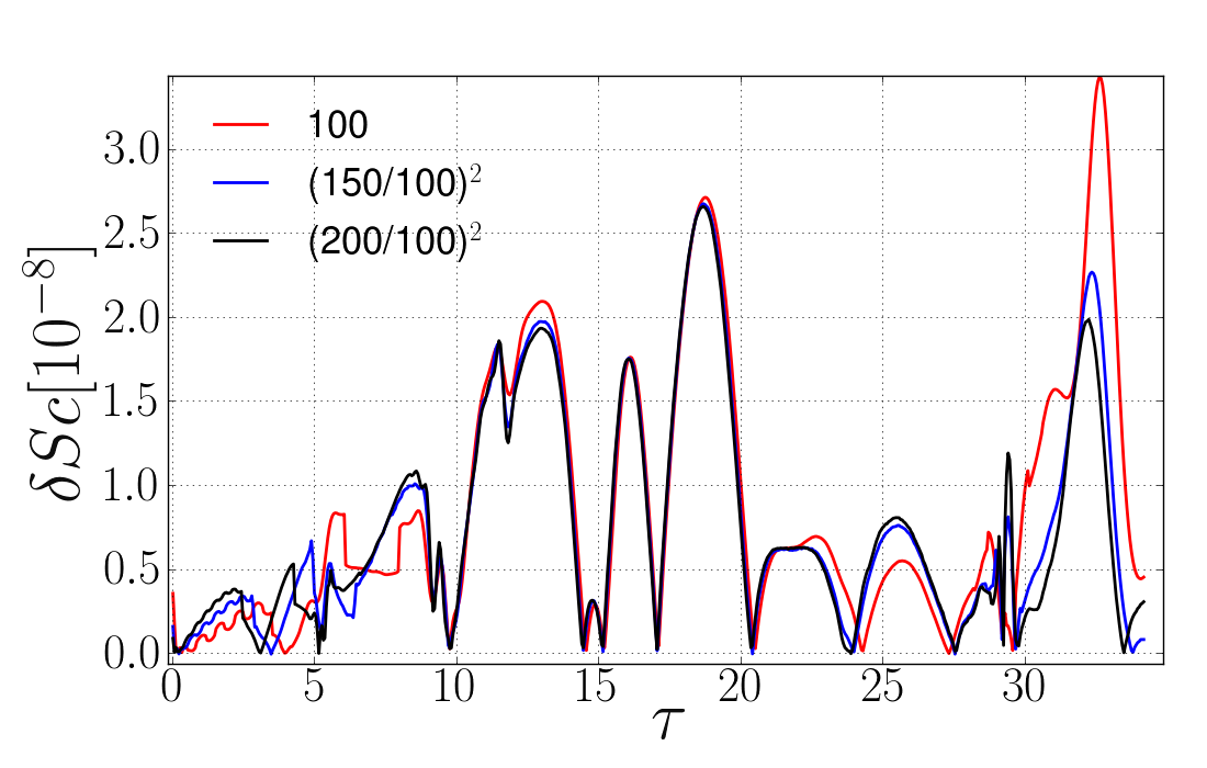
Finally, we evolved a set of geodesics in Kerr spacetime in quasi-isotropic coordinates Brandt and Seidel (1996) and fully nonlinear numerical evolutions of a Kerr BH starting with quasi-isotropic initial data. Here the two codes evolve the geodesics in gauges that rapidly deviate from each other. The effects of the unresolved gauge wave are apparent in the noise and lower-order convergence seen in Fig. 6. We see a similar lower order convergence when using Schwarzschild isotropic data.

Figure 6: Second-order convergence of the gauge independent curvature eigenvalues (Sc) as calculated using a fully nonlinear numerical evolution of Kerr data using the EinsteinToolkit, and as calculated using the exact Kerr metric in quasi-isotropic coordinates.

IV Results

The main analysis of this paper concerns the dynamics of geodesics on spacetimes obtained by numerically evolving (using CCZ4) initial data obtained from the analytic metric at various starting separations. In particular, we compare those geodesics with the ones obtained by solving the geodesic equation on the analytic spacetime. The differences between the numerically evolved metric and the analytic one arise from the differences in the Ricci tensor of the two. The CCZ4 algorithm drives the constraint violation toward small values, at which point the evolved metric is consistent with $T_{\mu\nu}=0$. The analytic metric, on the other hand, has $T_{\mu\nu}\neq 0$. Differences in $T_{\mu\nu}$ exist even at $t=0$, which means that the Riemann tensor on the initial slice is not the same between the numerical and analytic metrics.

We use the EinsteinToolkit to evolve geodesics on spacetimes obtained by using the analytic metric, with $m_{1}=m_{2}=M/2$, as initial data with separations of $D=50M$, $25M$, $20M$, $15M$, and $10M$. We simultaneously evolve these geodesics using our stand-alone C++ code with the purely analytic metric.

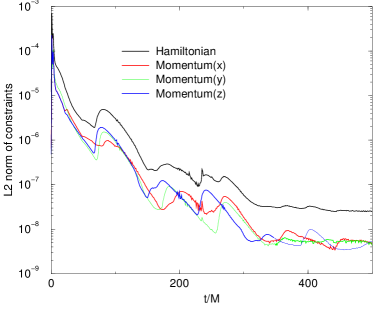
In Fig. 7, we show how the constraint violations decay with time using the CCZ4 evolution code (we see a decrease of over three orders of magnitude).

Figure 7: The L2 norm of the constraints for the $D=25M$ configuration. Here the constraints are calculated within the volume outside the two horizons and inside the coordinate sphere $r=30M$.

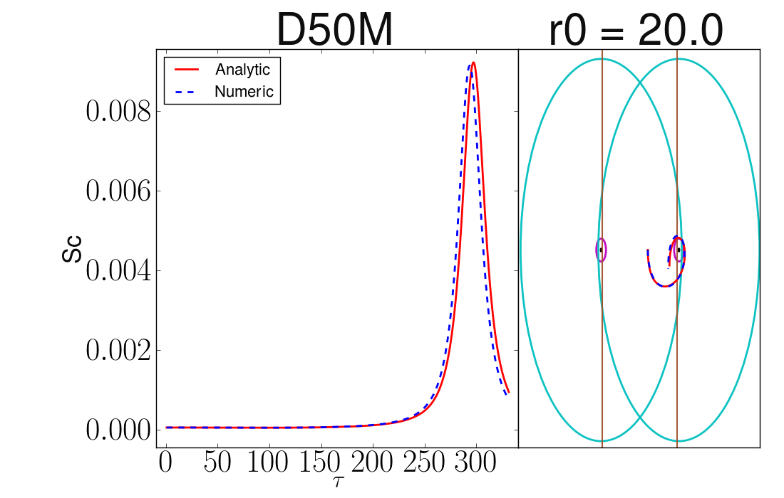
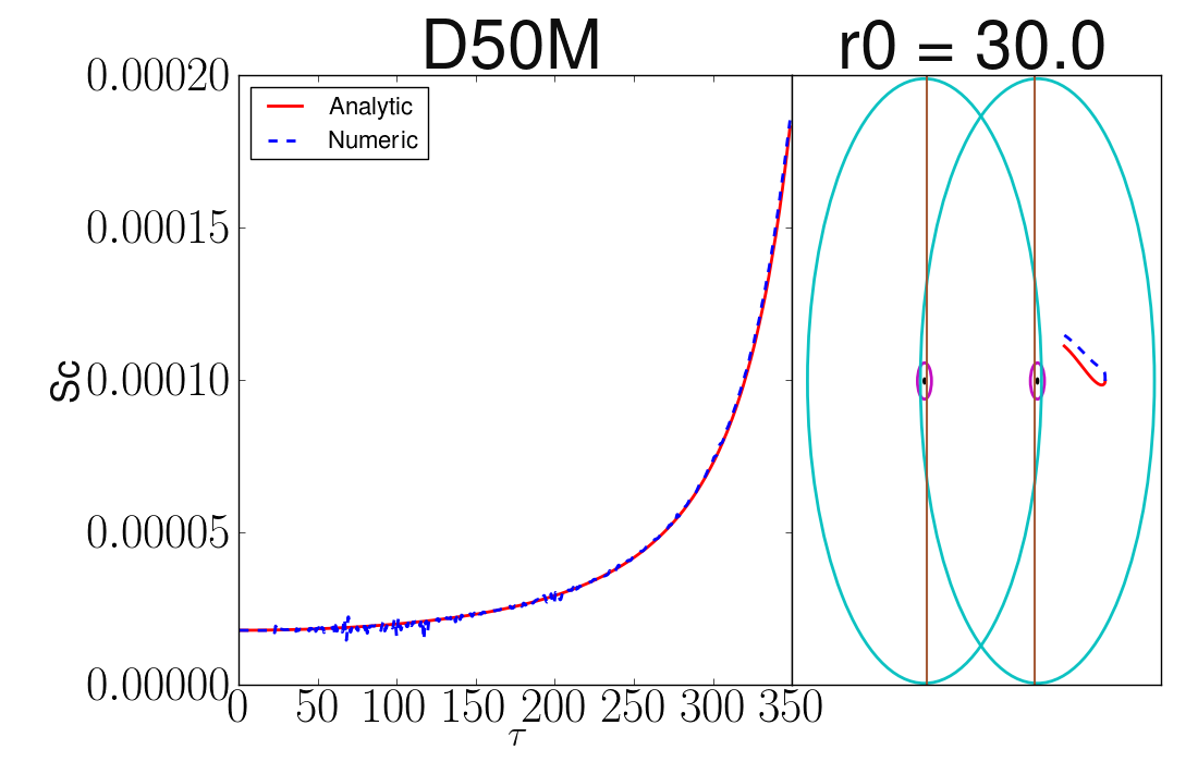
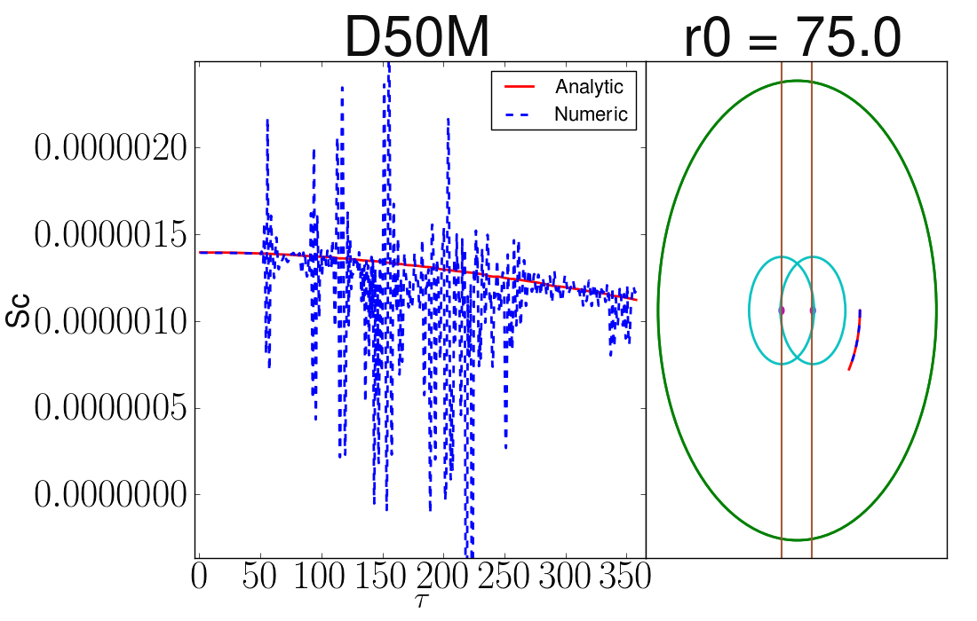
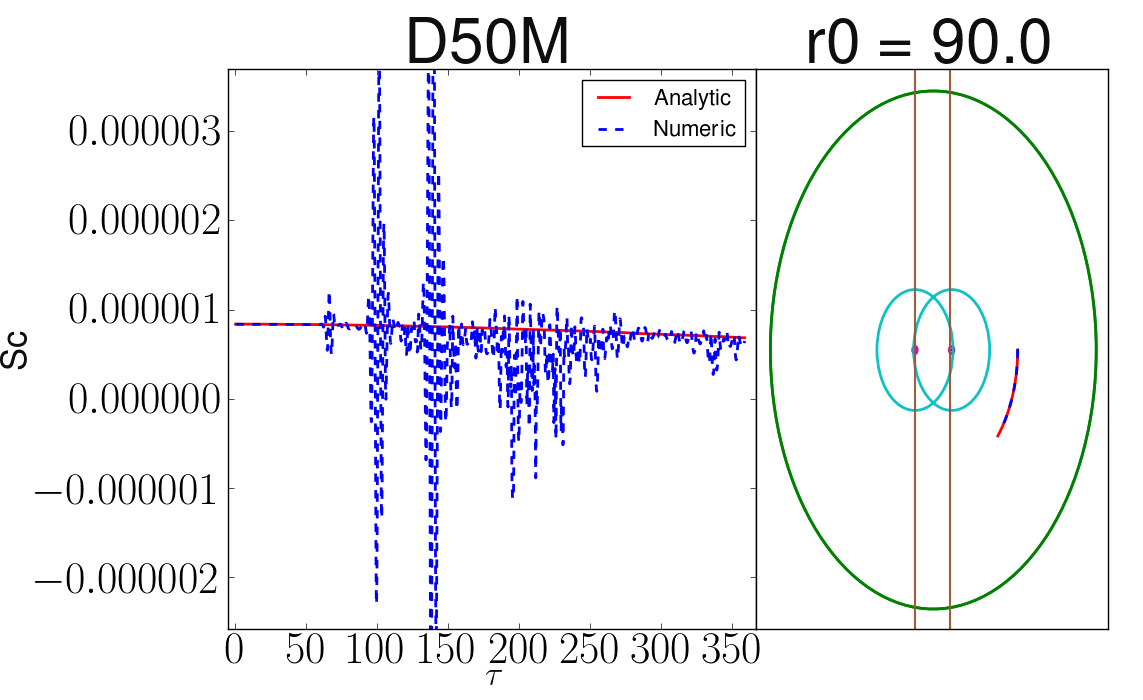
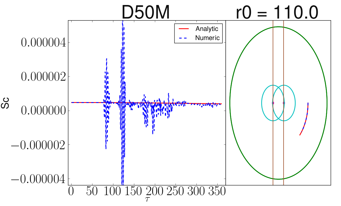
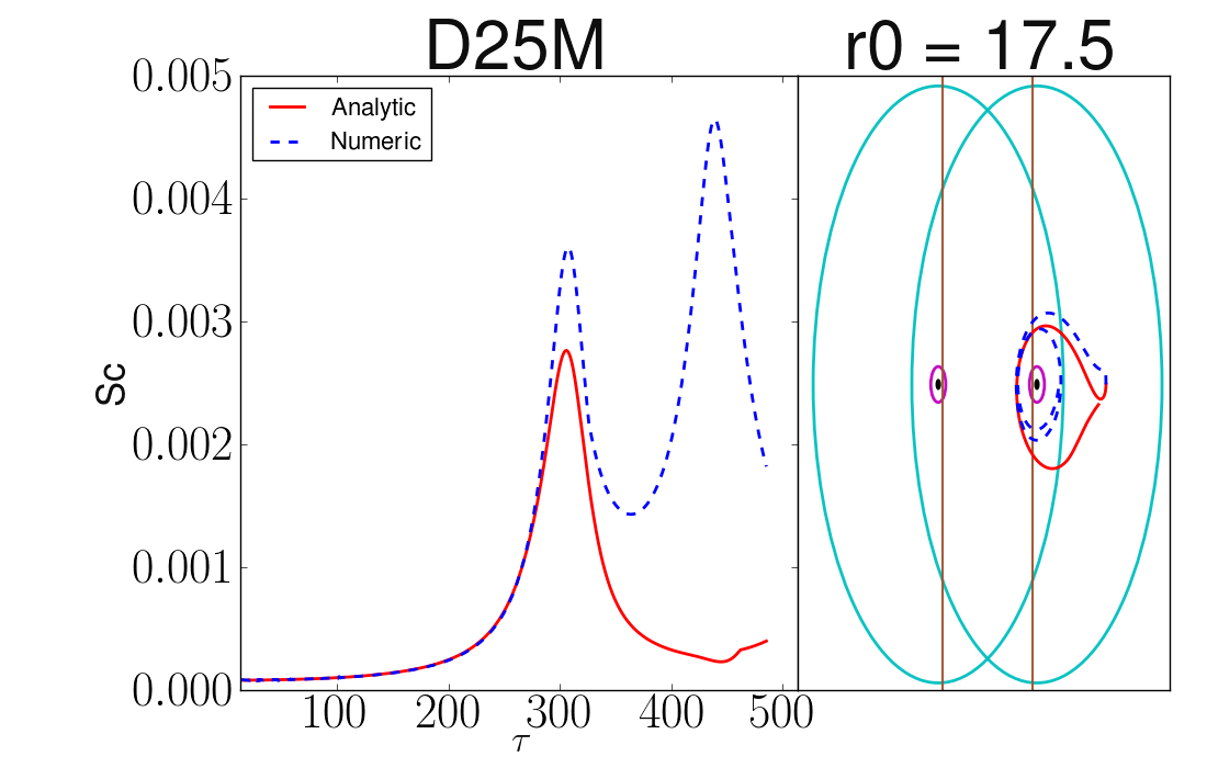
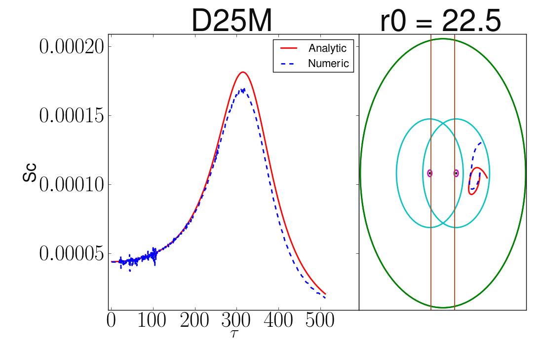
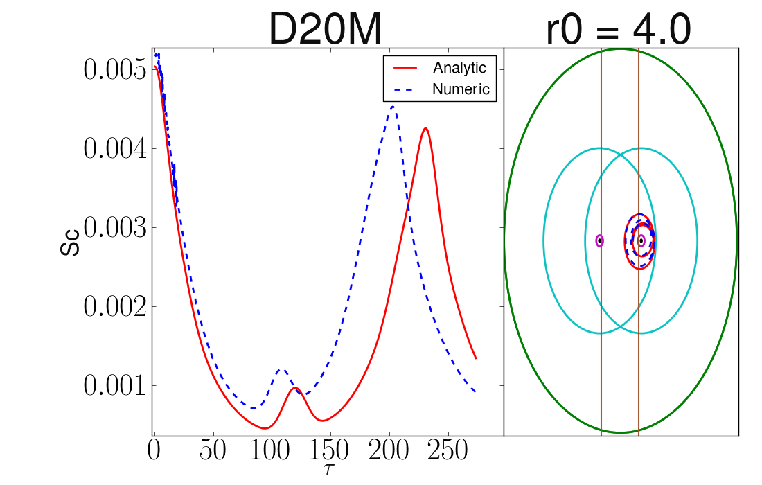
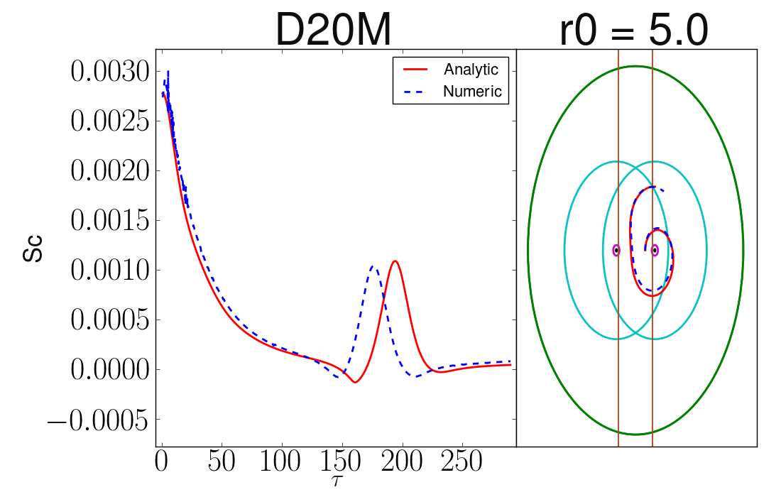
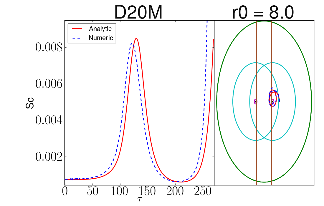
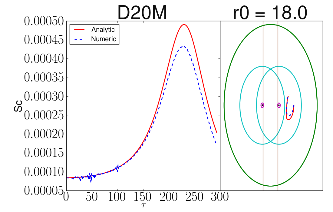
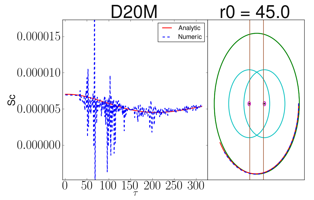
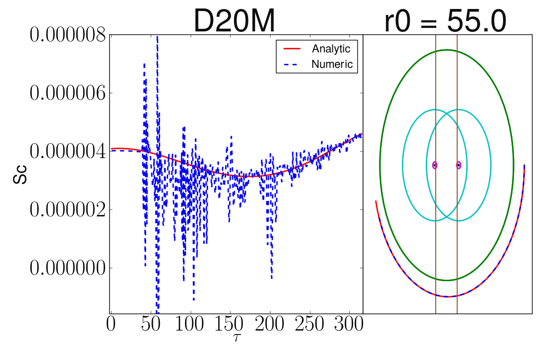
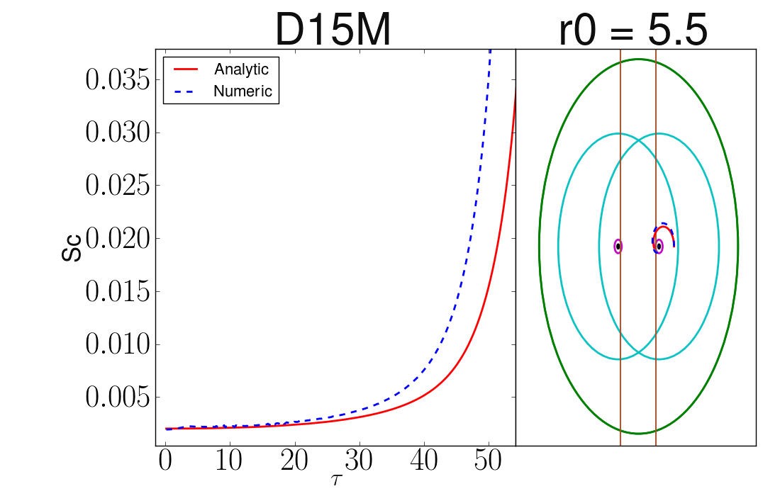
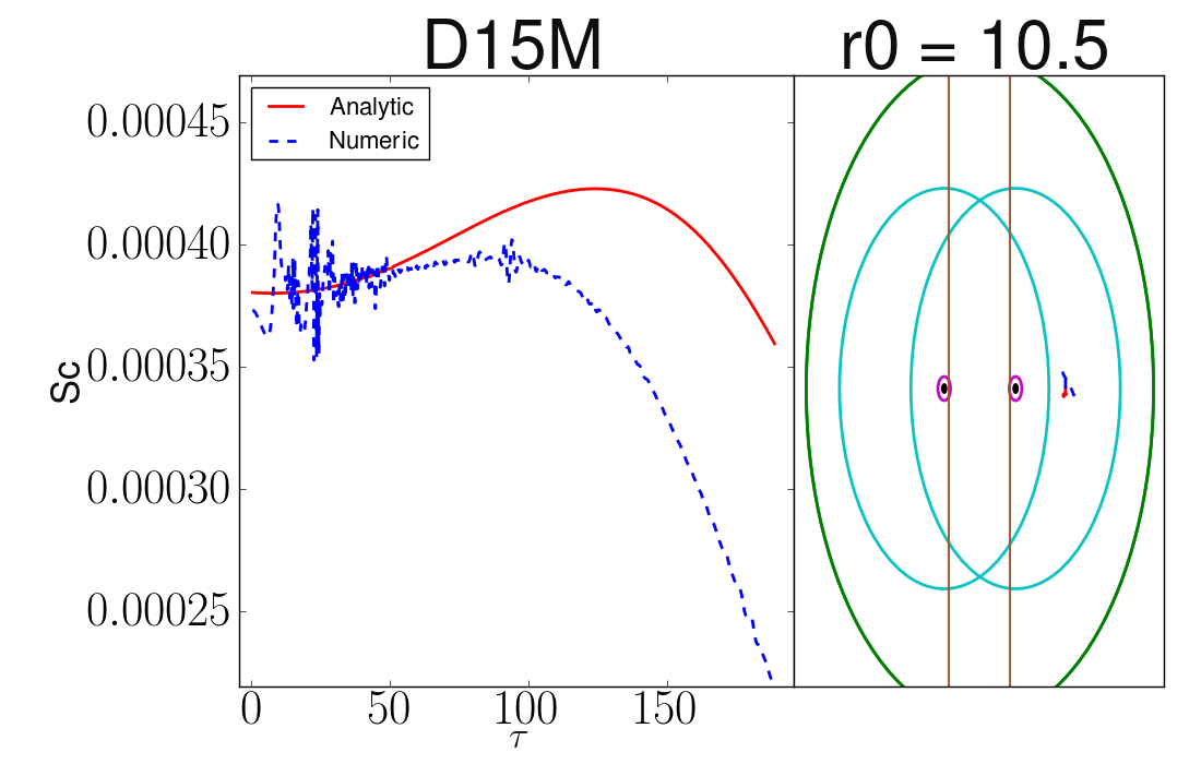
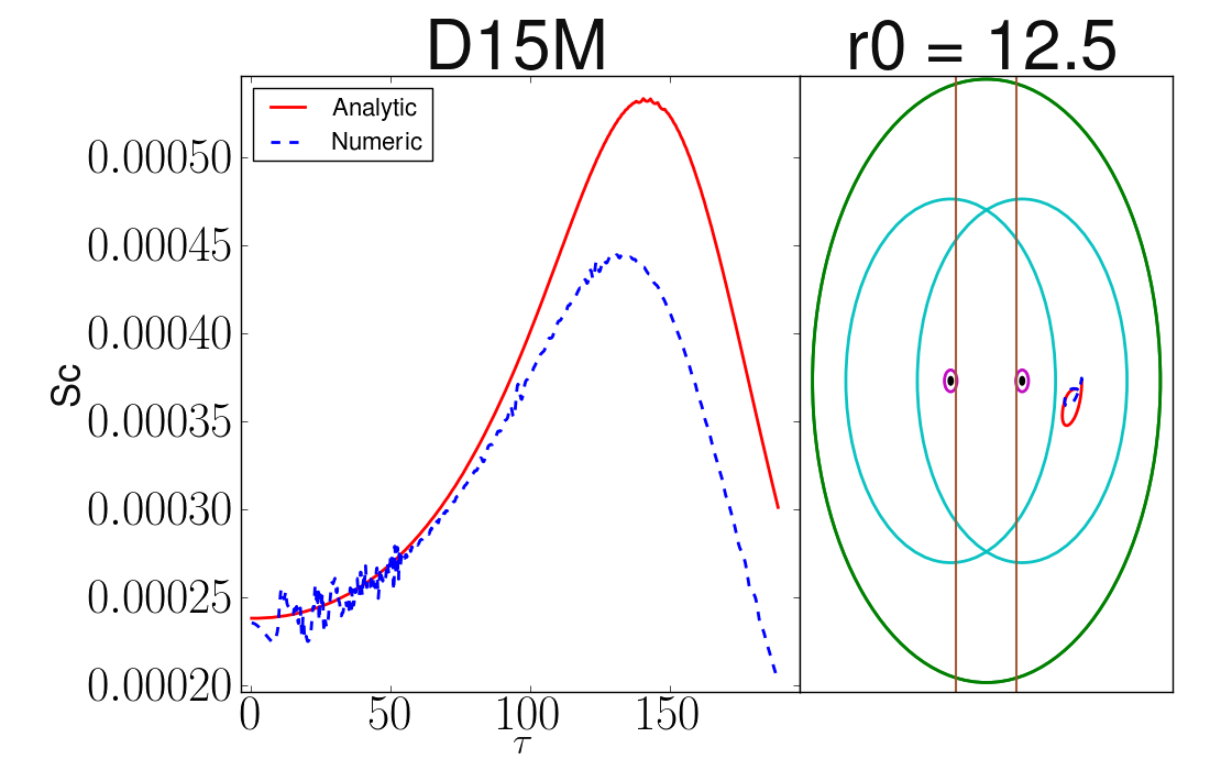
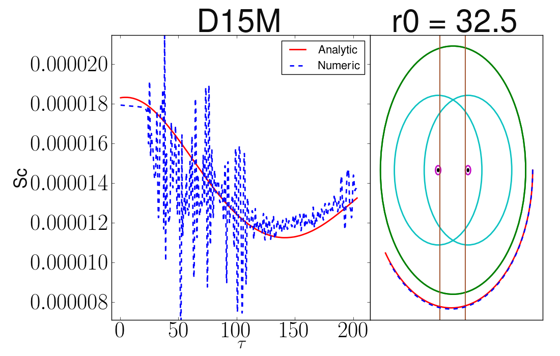
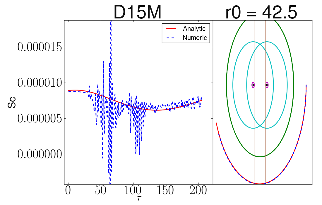
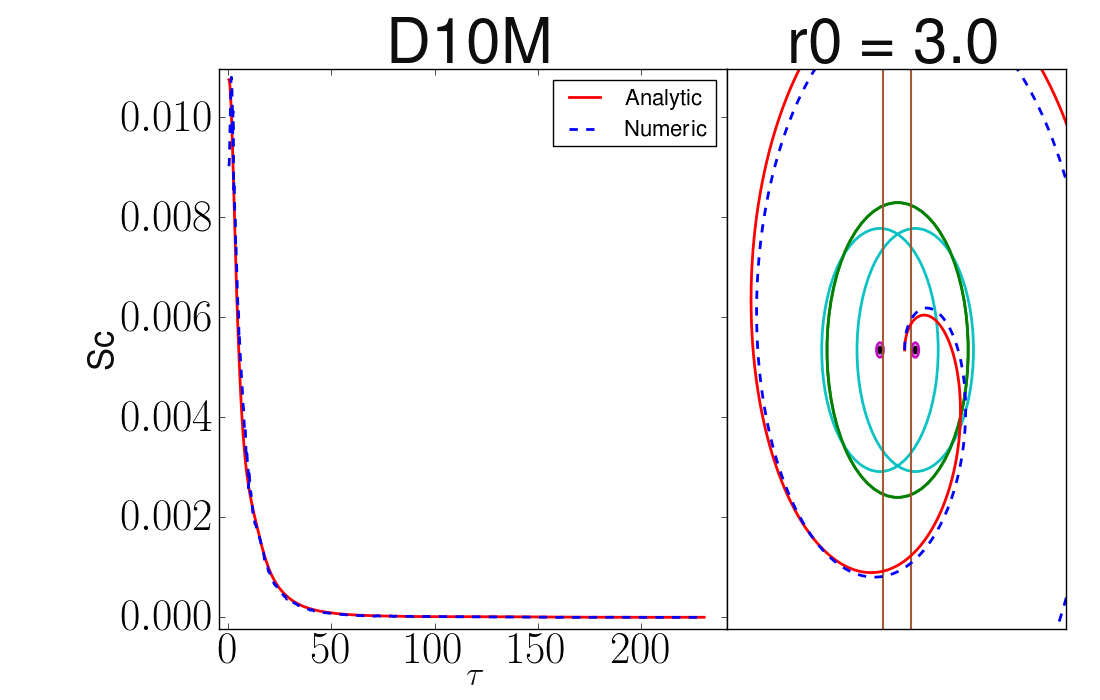
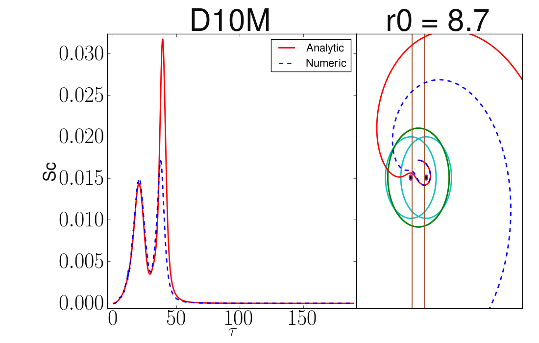
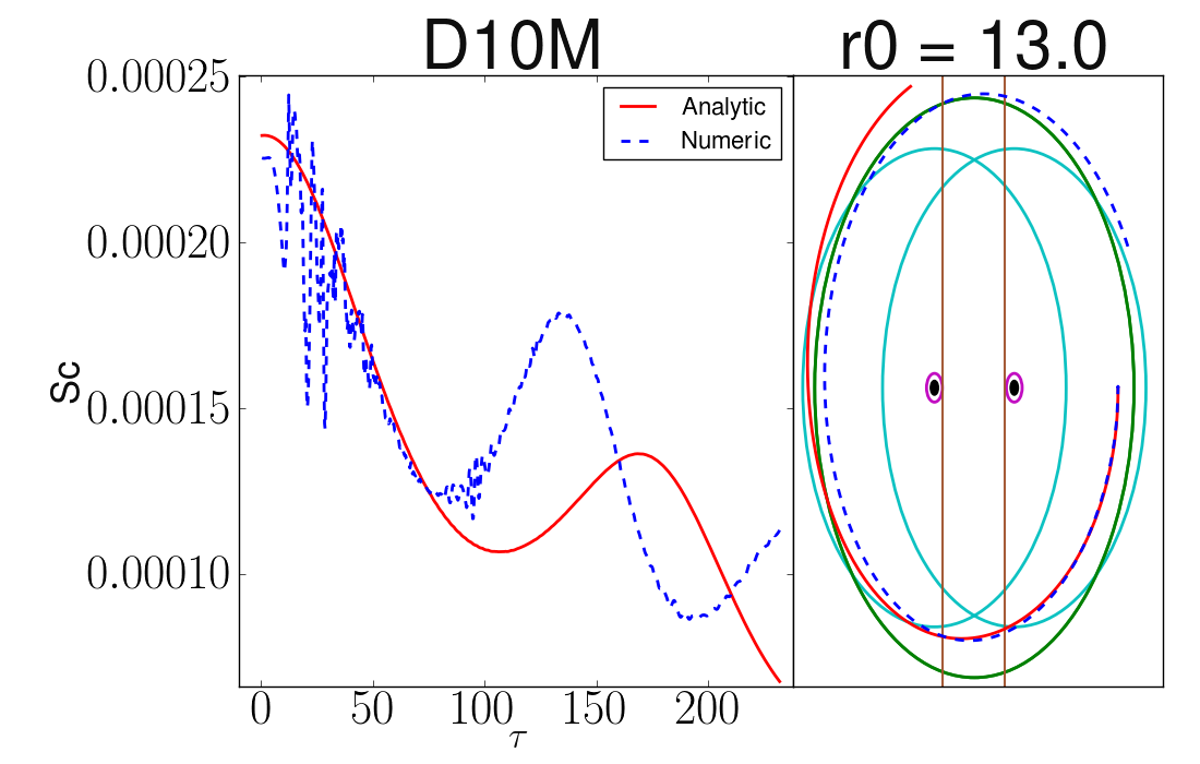
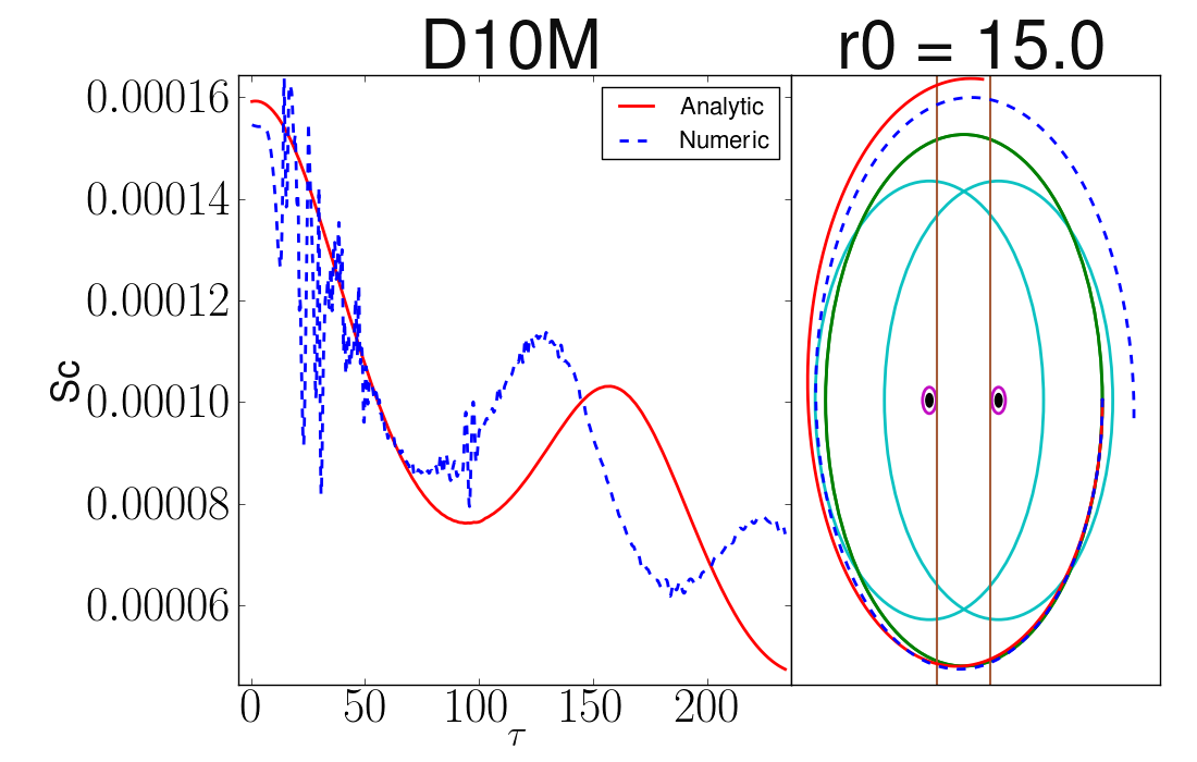
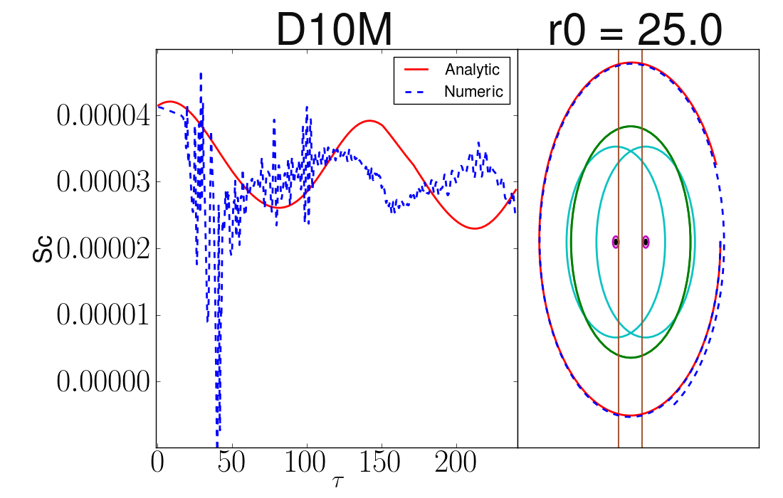
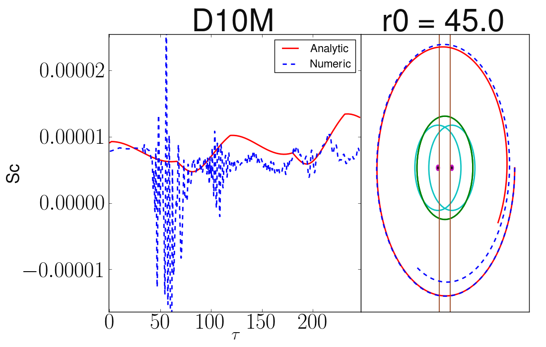
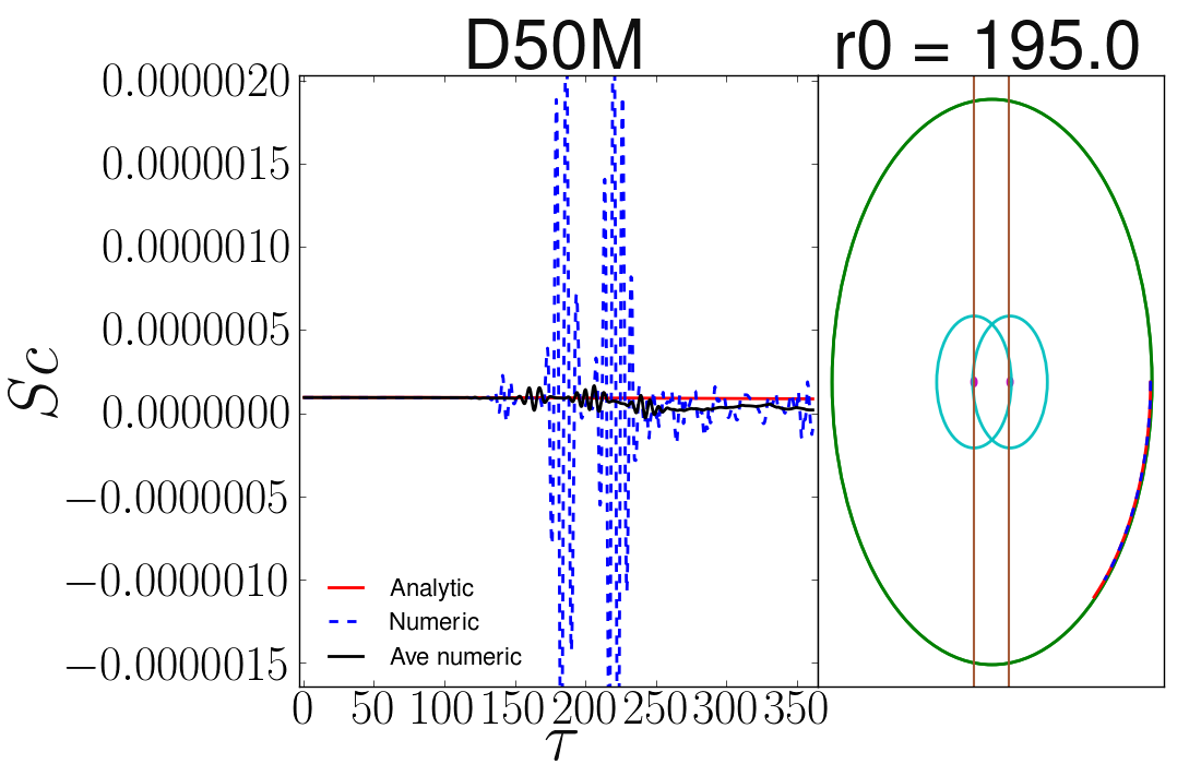
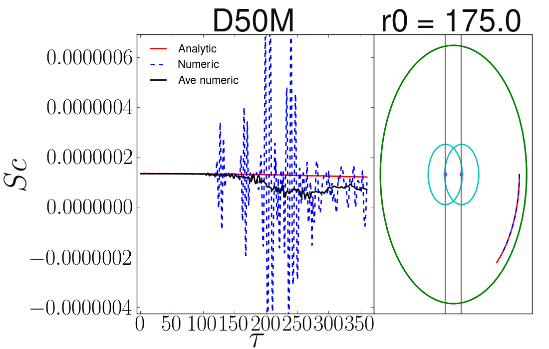
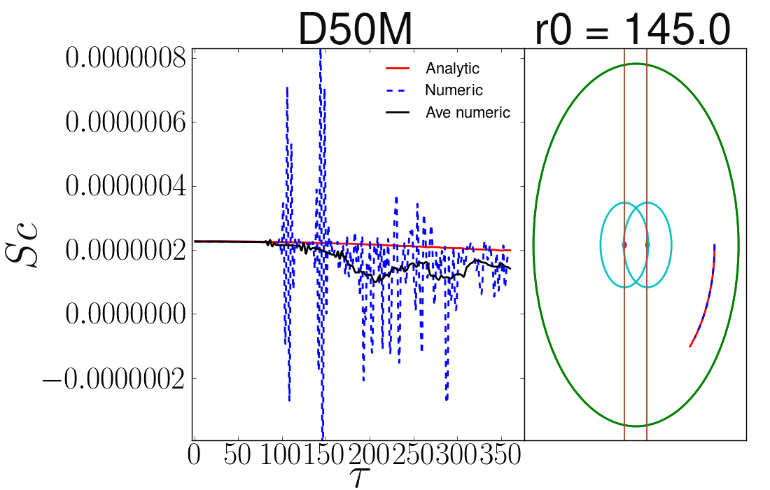
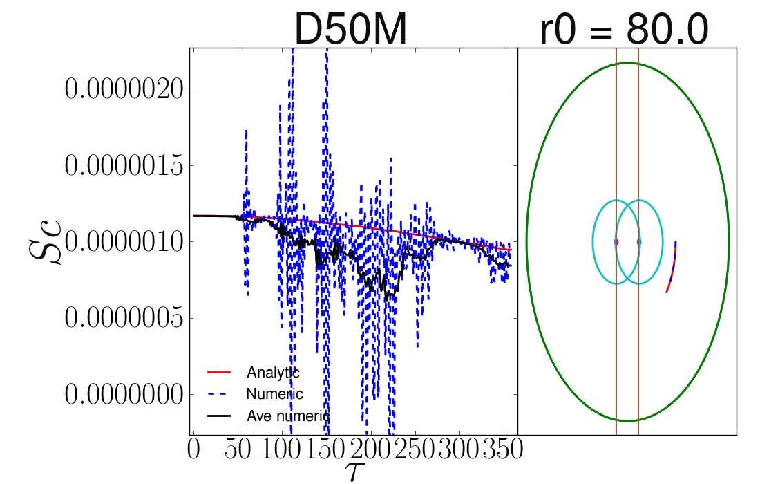
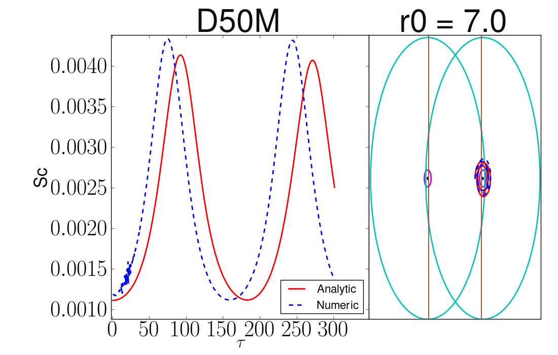
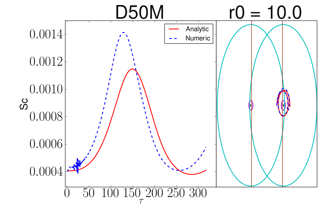
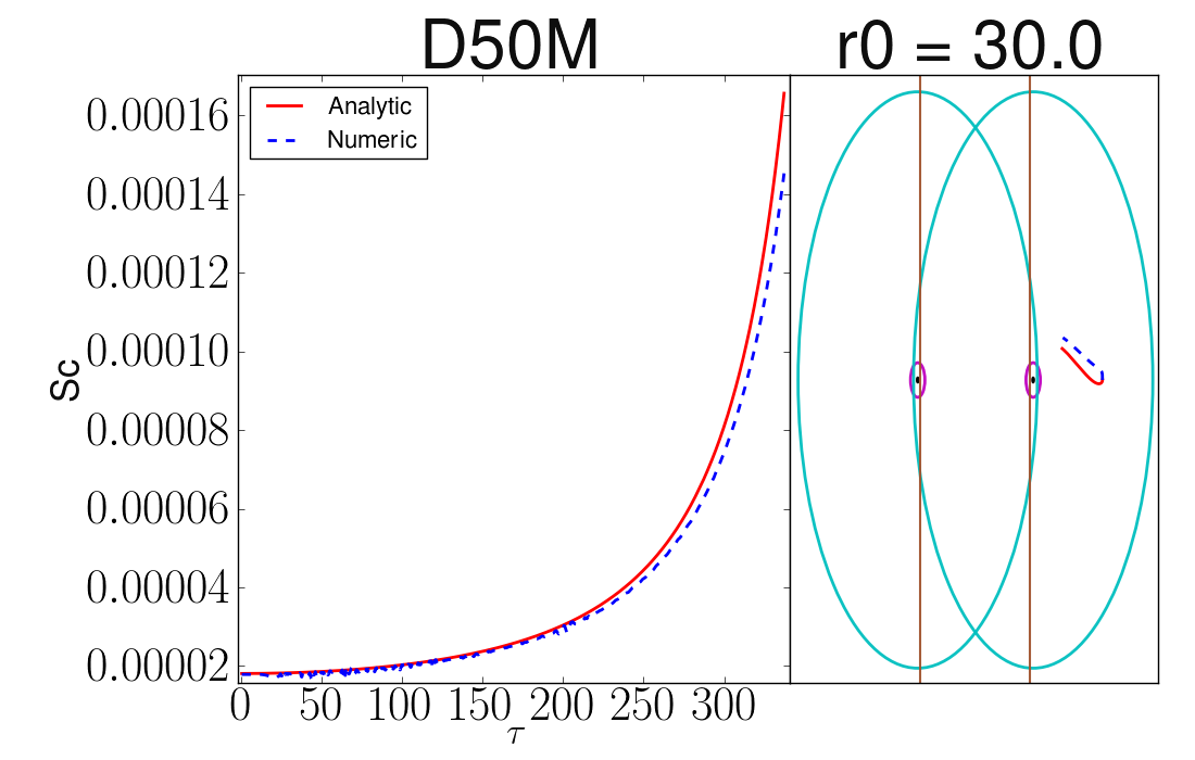
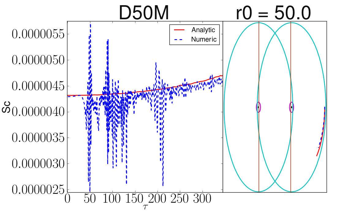
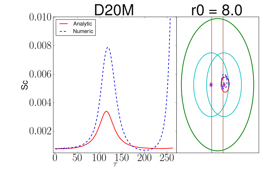
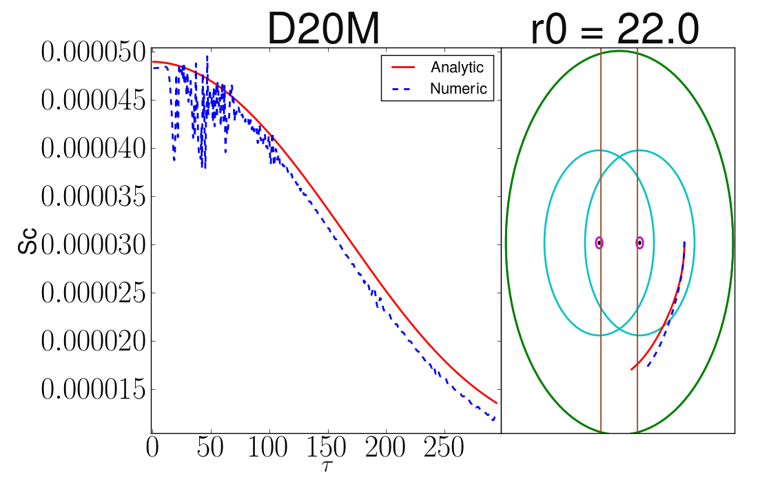
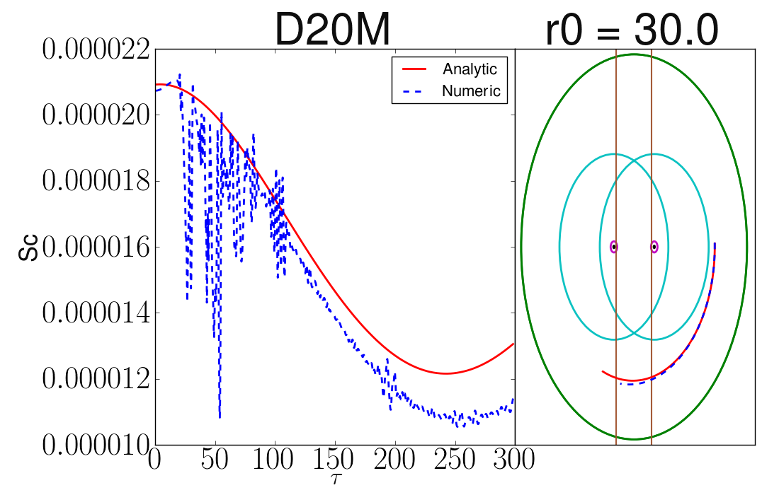
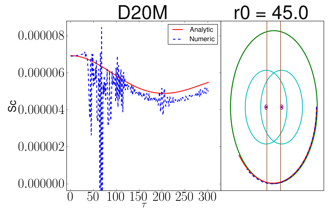
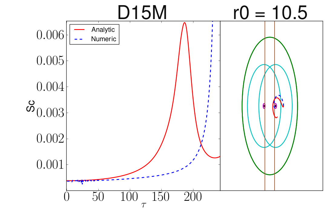
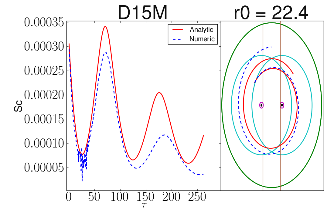
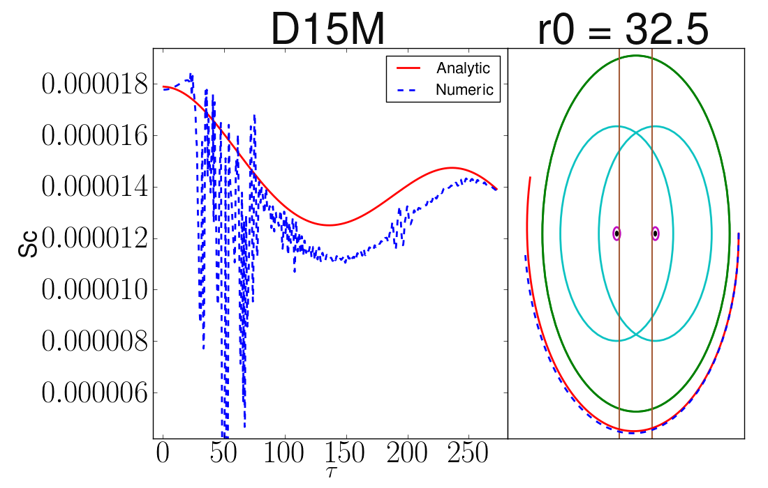
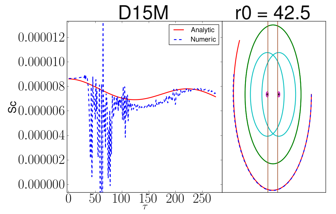
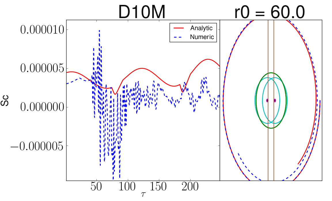
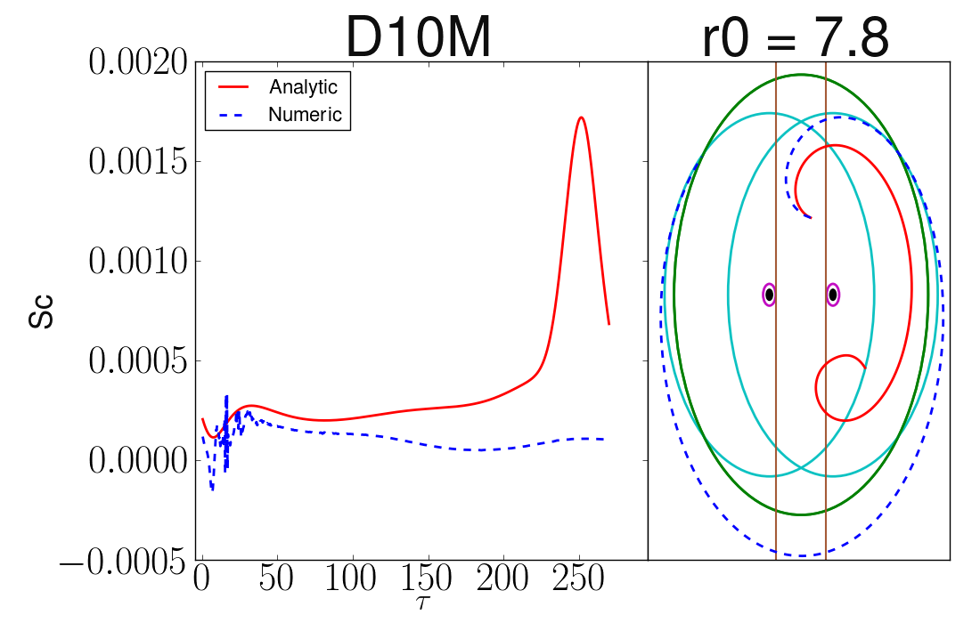
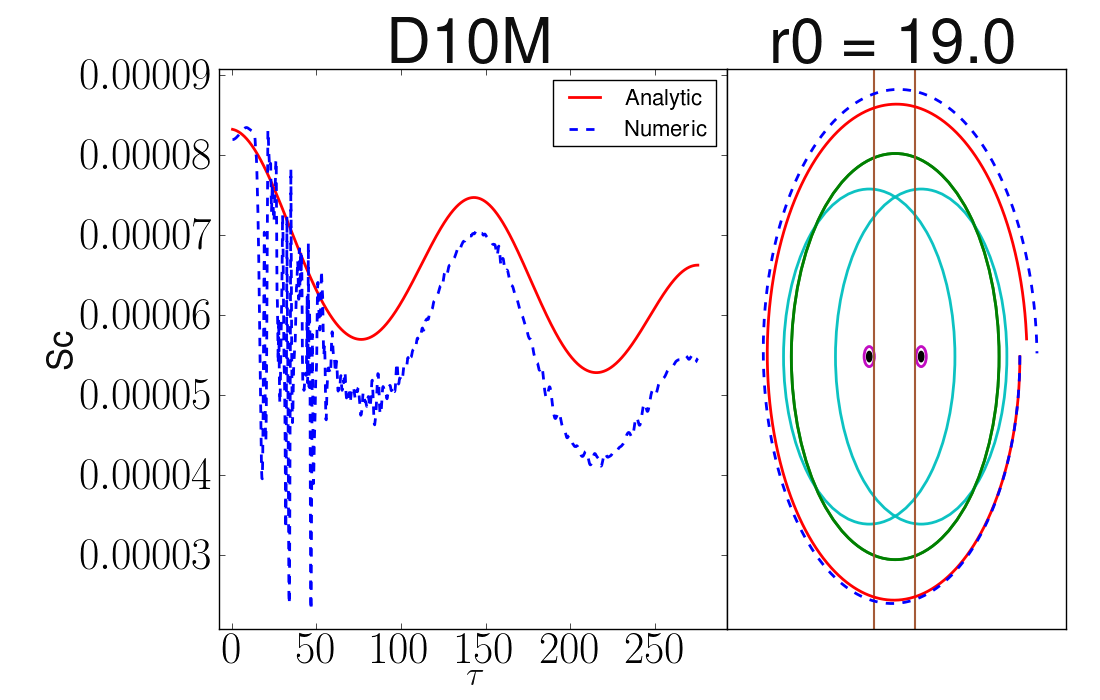
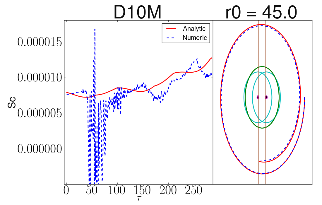
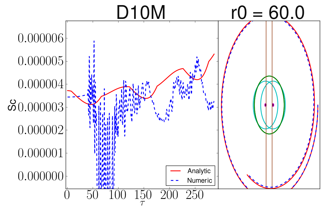
The results from a wide variety of geodesics are shown in Figs. 8, 9, and 10. The figures show one of the curvature eigenvalues (Sc) versus proper time, $\tau$, for various starting configurations. The coordinate trajectories of the geodesics in a corotating frame are also shown. The boundaries of the inner, near, far, and buffer zones are denoted by vertical lines and ellipses.

Figure 8: Separation $D=50M$ results. Here we plot the value of the largest (in magnitude) curvature eigenvalue (Sc) versus time (as evolved using the numerical and analytic metric), as well as plot the coordinate position of the geodesics in a corotating frame (i.e., one where the BH positions are nearly fixed) on the right side of each panel. The vertical lines and circles in these trajectory plots show the location of the various zones described in Sec. II.1. The number $r_{0}$ (normalized by $M$) is the initial coordinate distance of the geodesic from the nearest BH. For the geodesics close to the BHs, the noise in the numerically evolved spacetime is low compared to the magnitude of the curvature eigenvalues, the opposite is true for the farthest ones.

Figure 9: Separation $D=25M$ and $D=20M$ results. Here we plot the value of the largest (in magnitude) curvature eigenvalue (Sc) versus time (as evolved using the numerical and analytic metric), as well as plot the coordinate position of the geodesics in a corotating frame (i.e., one where the BH positions are nearly fixed) on the right side of each panel. The vertical lines and circles in these trajectory plots show the location of the various zones described in Sec. II.1. The number $r_{0}$ (normalized by $M$) is the initial coordinate distance of the geodesic from the nearest BH. For the geodesics close to the BHs, the noise in the numerically evolved spacetime is low compared to the magnitude of the curvature eigenvalues, the opposite is true for the farthest ones.

Figure 10: Separation $D=15M$ and $D=10M$ results. Here we plot the value of the largest (in magnitude) curvature eigenvalue (Sc) versus time (as evolved using the numerical and analytic metric), as well as plot the coordinate position of the geodesics in a corotating frame (i.e., one where the BH positions are nearly fixed) on the right side of each panel. The vertical lines and circles in these trajectory plots show the location of the various zones described in Sec. II.1. The number $r_{0}$ (normalized by $M$) is the initial coordinate distance of the geodesic from the nearest BH. For the geodesics close to the BHs, the noise in the numerically evolved spacetime is low compared to the magnitude of the curvature eigenvalues, the opposite is true for the farthest ones.

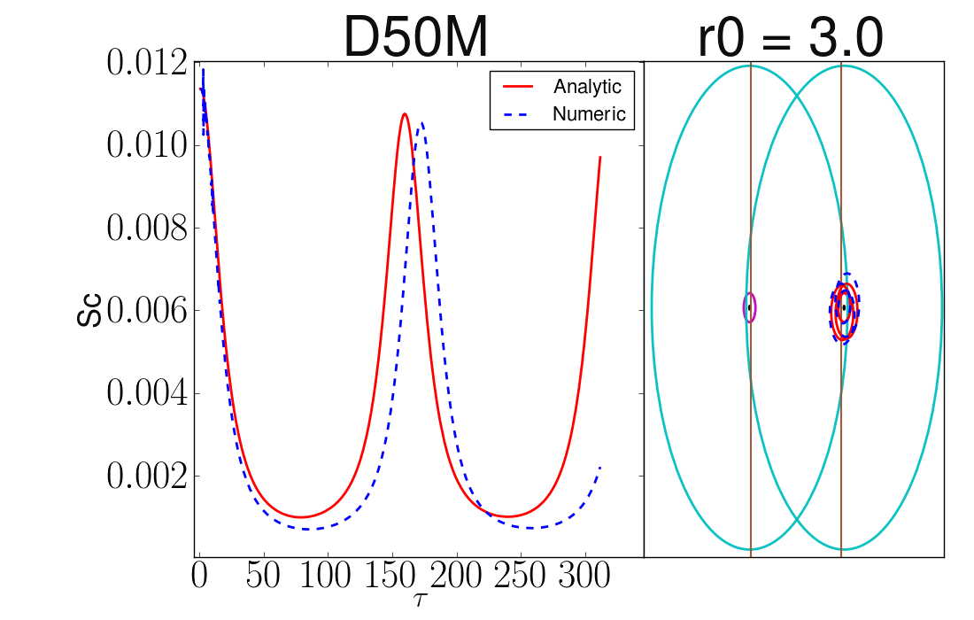
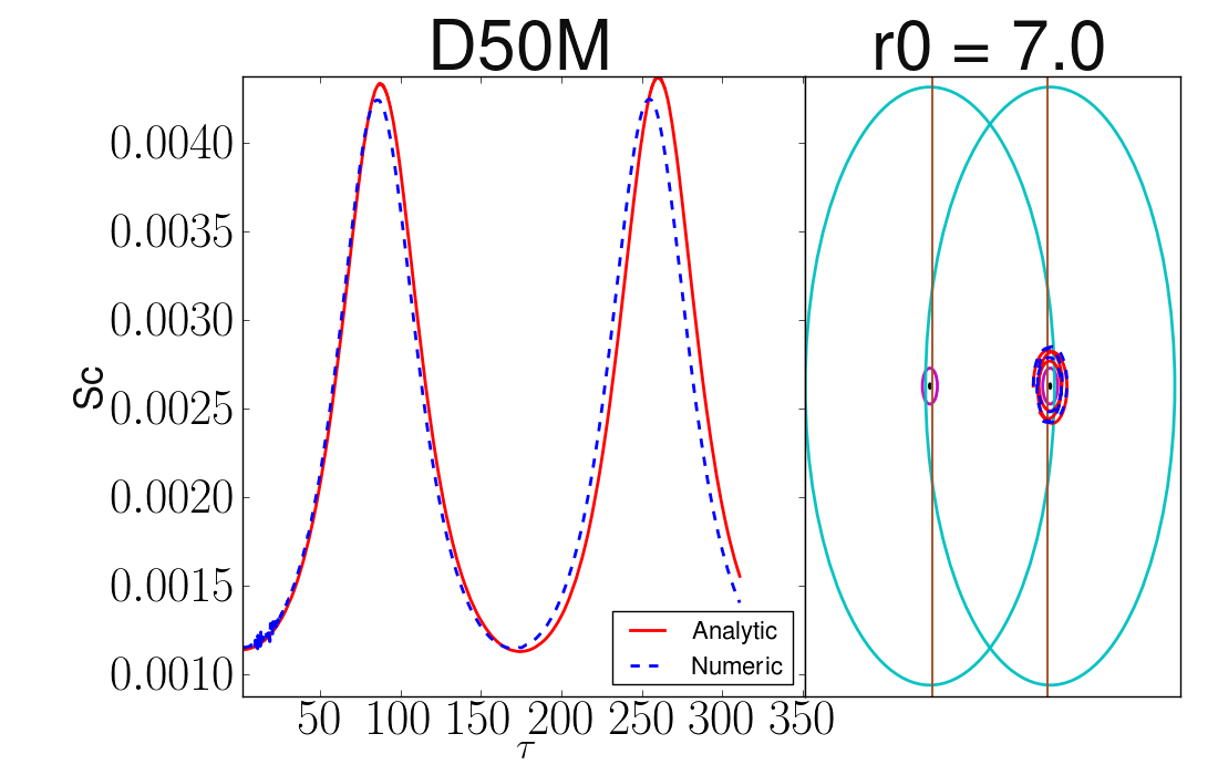
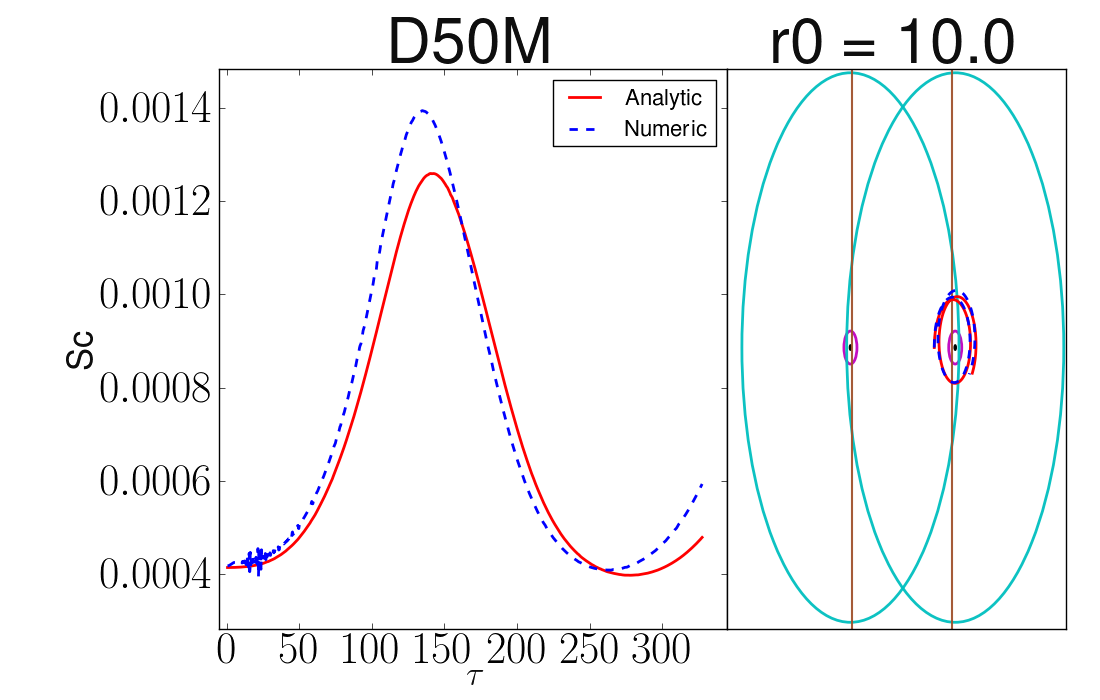
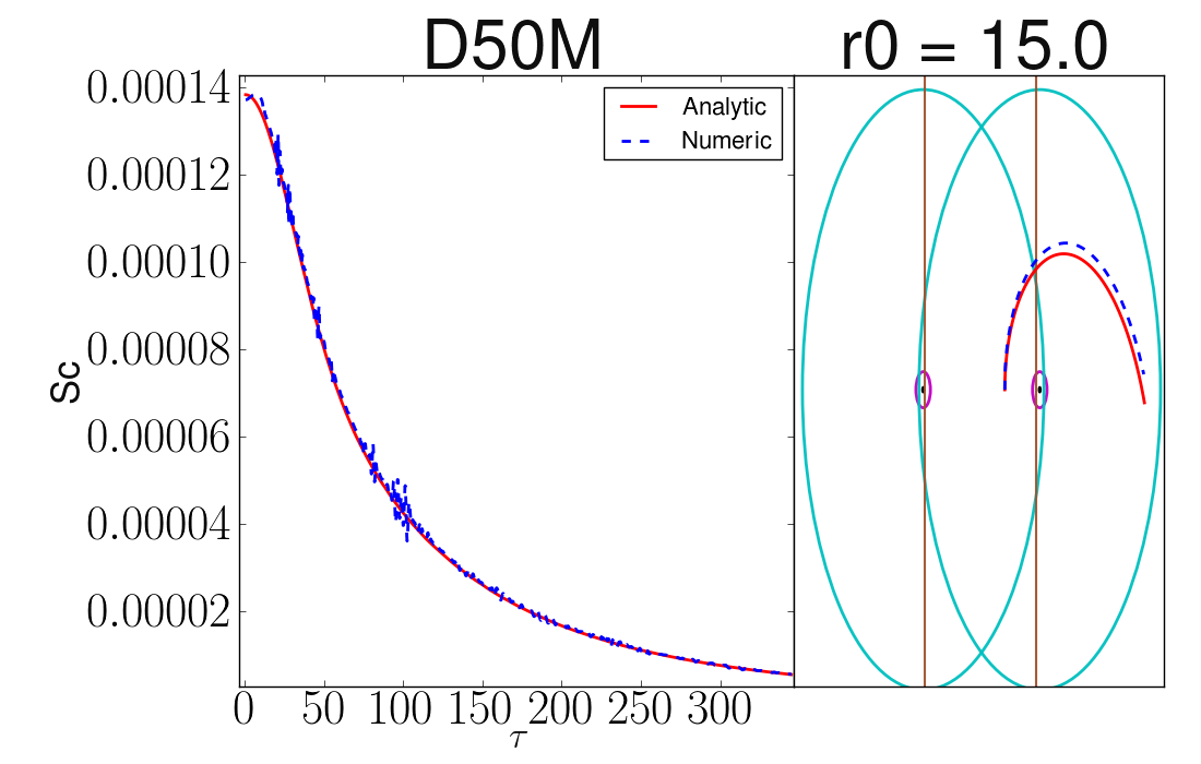
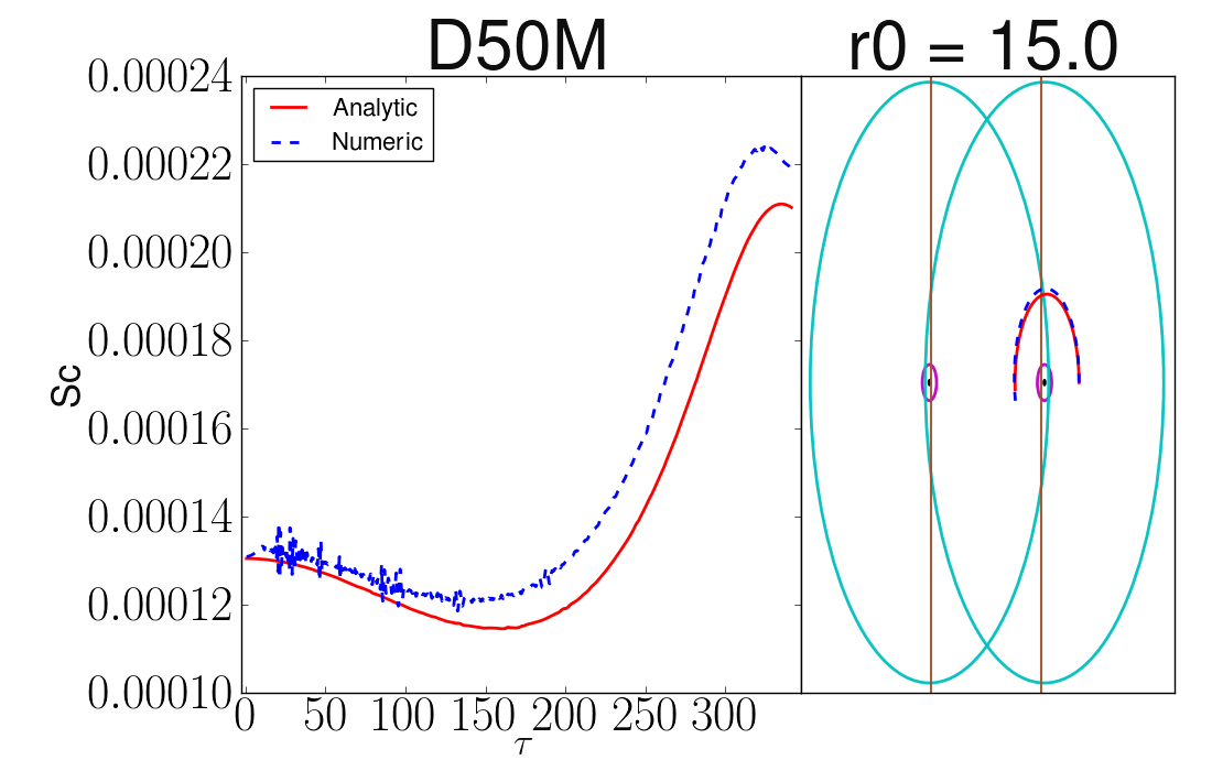
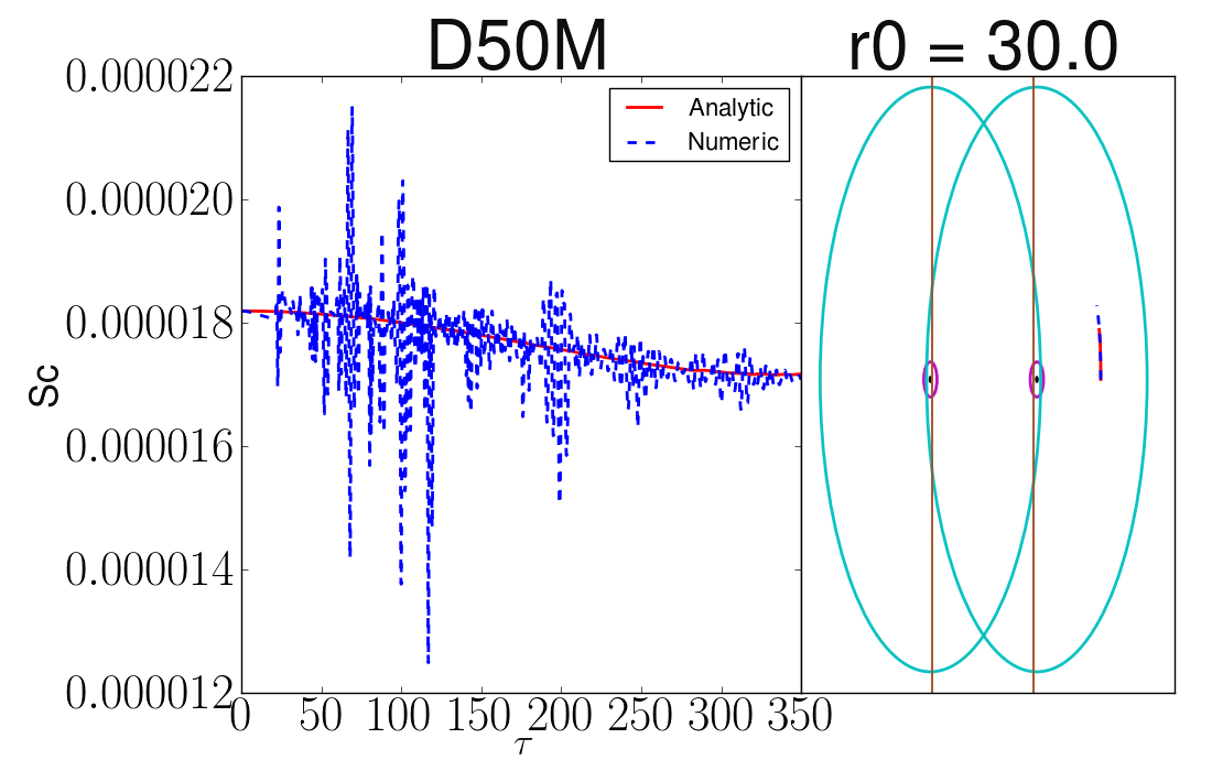
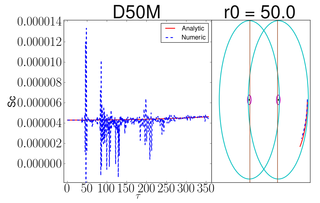
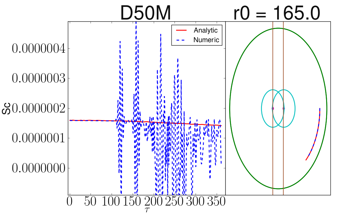
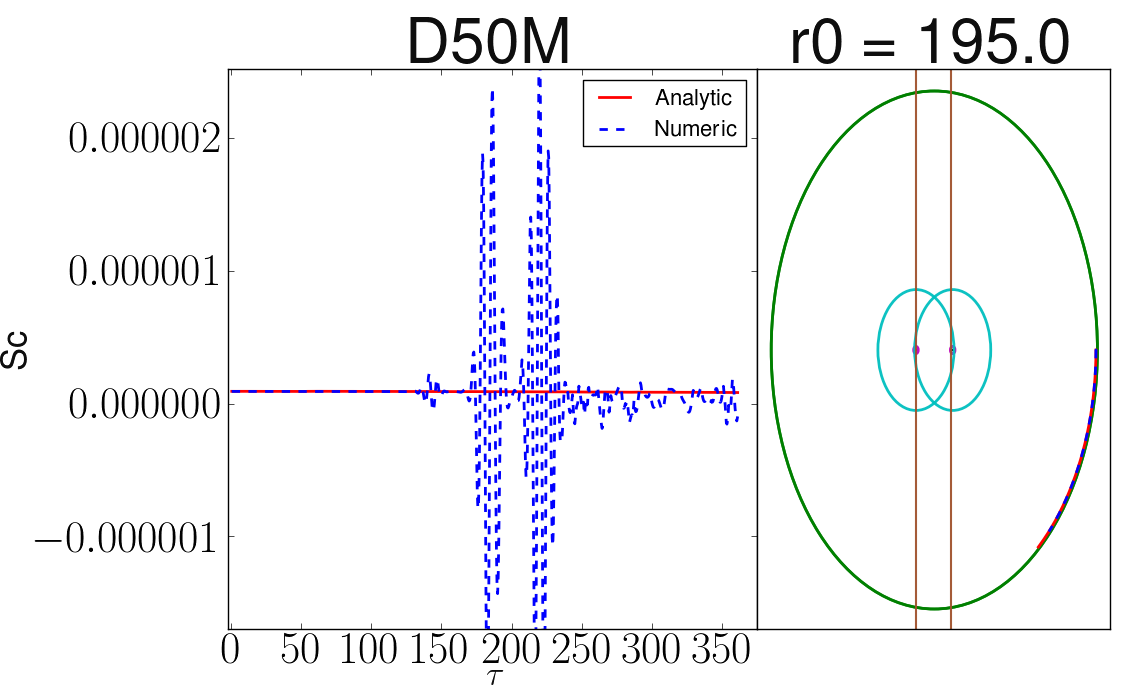
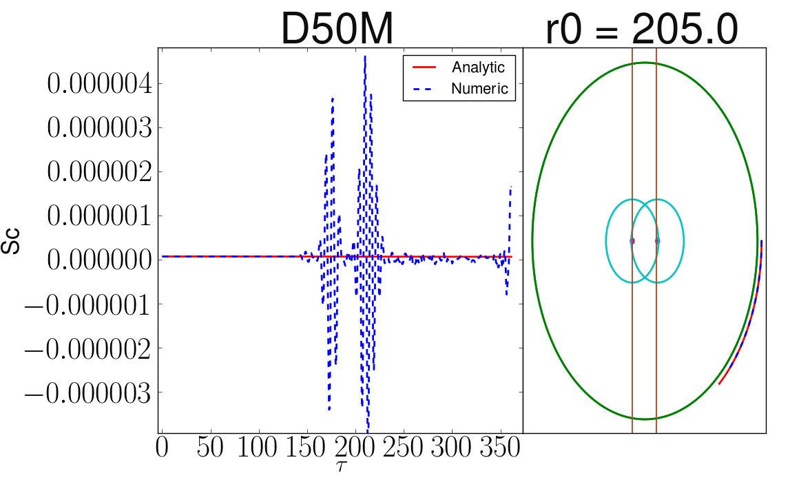
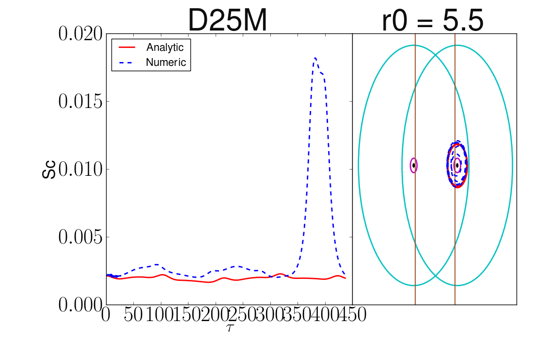
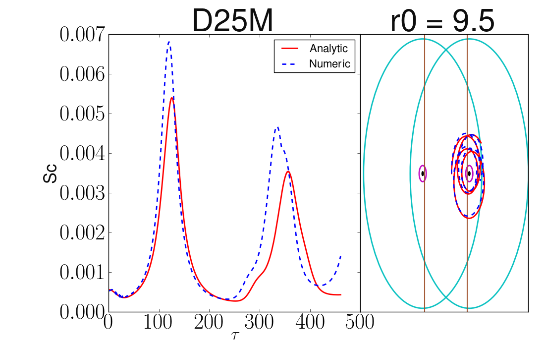
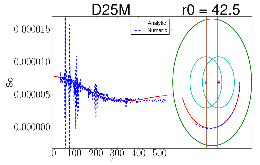
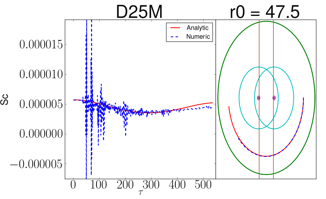
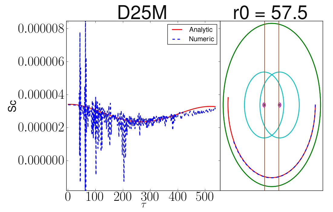
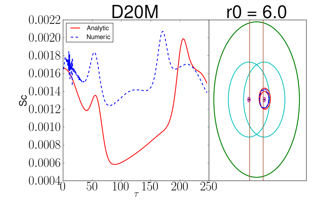
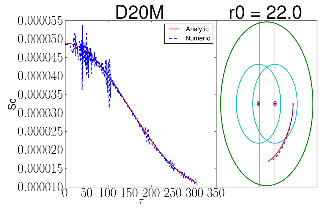
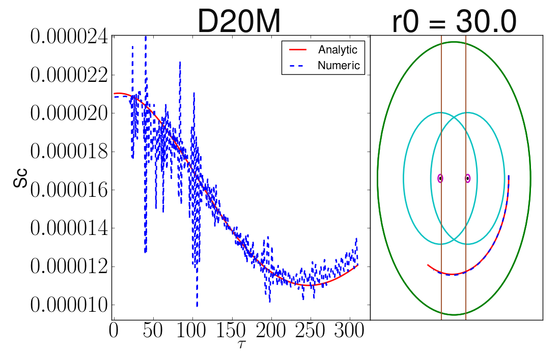
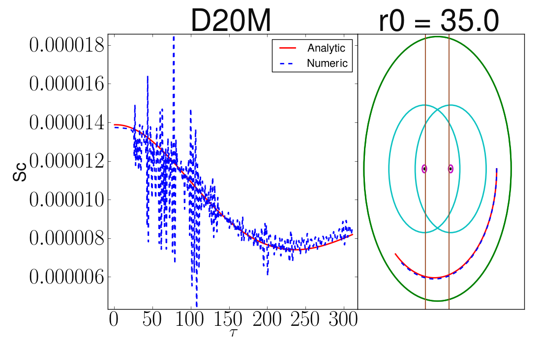
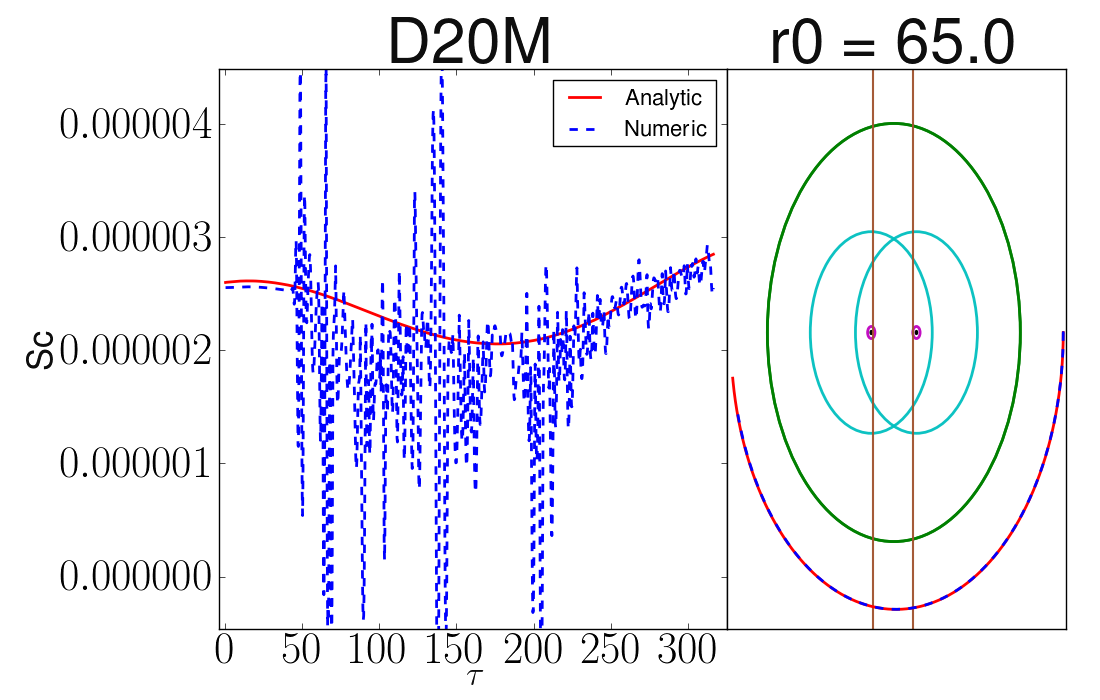
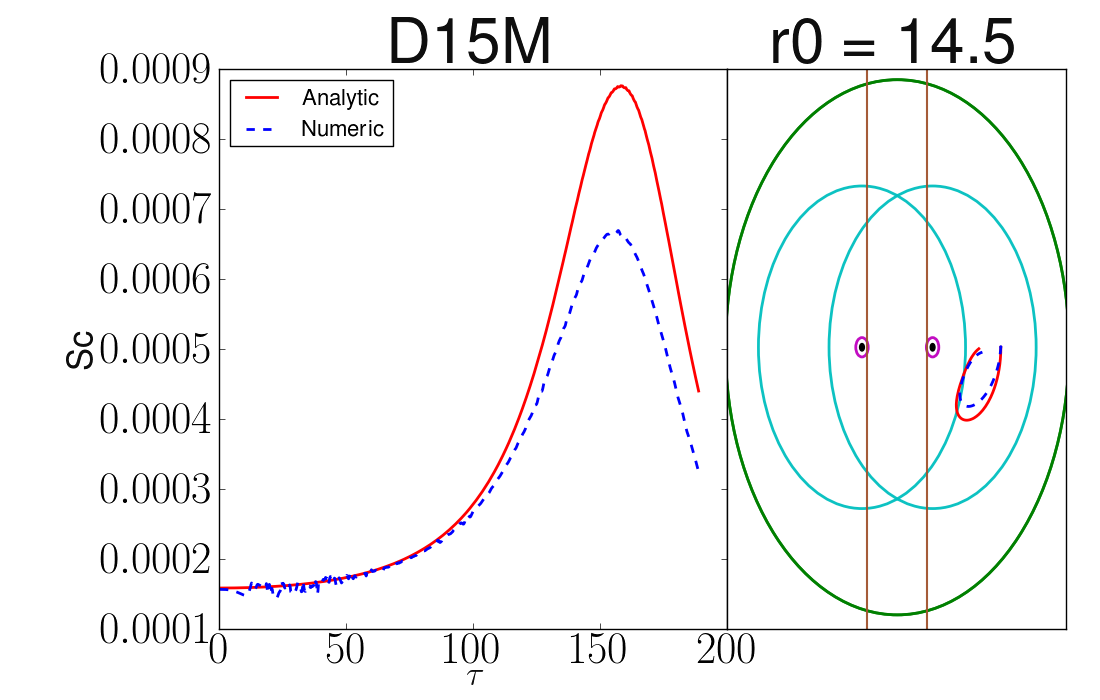
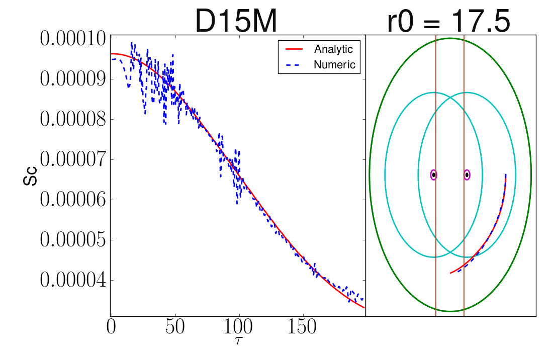
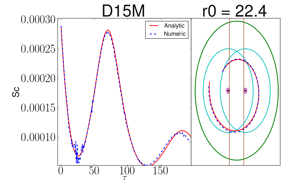
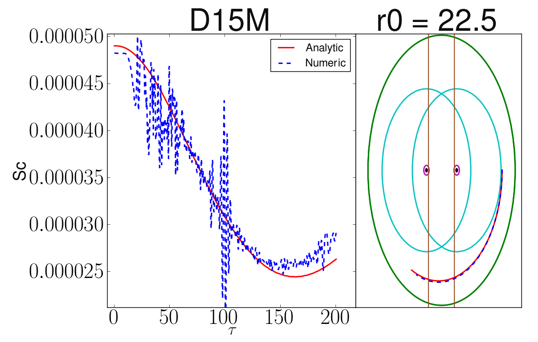
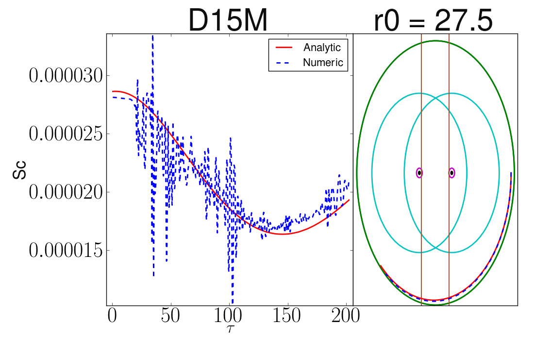
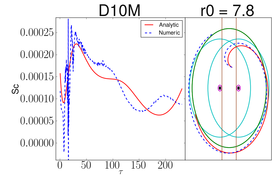
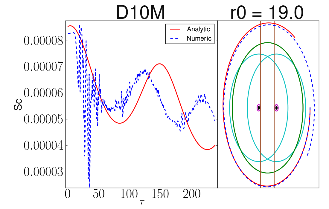
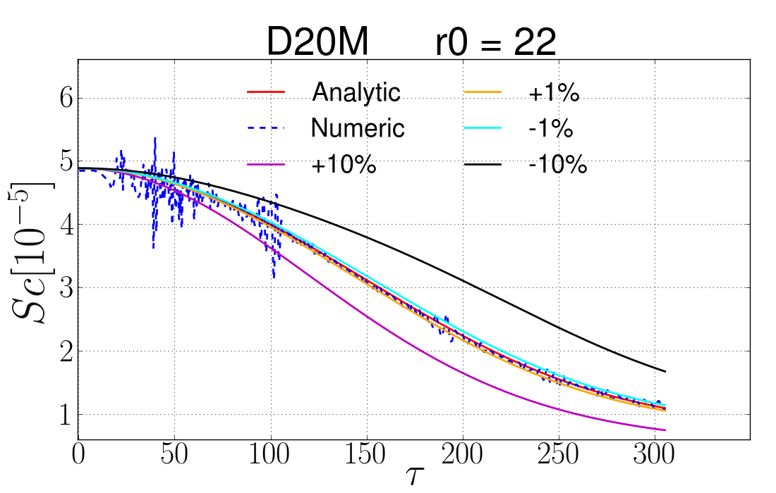
The noise apparent in the curvature eigenvalues for the geodesics far from the BHs is due reflections of spurious waves off of the AMR boundaries (this is the same error associated with high-frequency oscillations in the waveform seen in numerical evolutions of BHBs using AMR-based codes). At far distances, this noise is larger in magnitude than the curvature eigenvalues. See, for example, the $r_{0}\gtrsim 100M$ curves for the $D=50M$ configuration in Fig. 8.

At a separation of $D=50M$ in Fig. 8, one would expect very good agreement between the analytic metric and the numerical one. Quantitatively, there is remarkably good agreement when the geodesics are about $20M\lesssim r_{0}\lesssim 100M$ from the BHs. Closer than this, there are small, but noticeable differences, and farther than this, there is some evidence significant differences, but in those cases the noise is significantly larger than the curvature eigenvalues themselves.

We find that initial conditions that lead to nearly circular geodesics for one metric do lead to nearly circular geodesics for the other. The best agreement here are for geodesics in the outer regions of the inner-to-near-zone buffer regions and the near zone.

At a binary separation of $D=25M$ (see Fig. 9), the disagreement between the analytical and numerical results when the geodesics are close are exacerbated. Good agreement between the curvature eigenvalues is still apparent in the outer part of the inner-to-near zone buffer region and the near zone, although at late times these geodesics show deviations as shown for the $r_{0}>40M$ cases. At a binary separation of $D=10M$ (see Fig. 10), there are noticeable differences in the curvature eigenvalues for almost all geodesics. However, examining the $D=15M$ geodesics (see Fig. 10) shows something perhaps surprising. The geodesics in the outer part of the inner-to-near zone buffer region and the near zone are remarkably good. Here, the deviations for far geodesics also start to deviate at later times. It seems these deviations are dependent on the binary separation. One may have expected these geodesics to be substantially worse than the $D=25M$ and $D=20M$ analogs, but we do not see this.

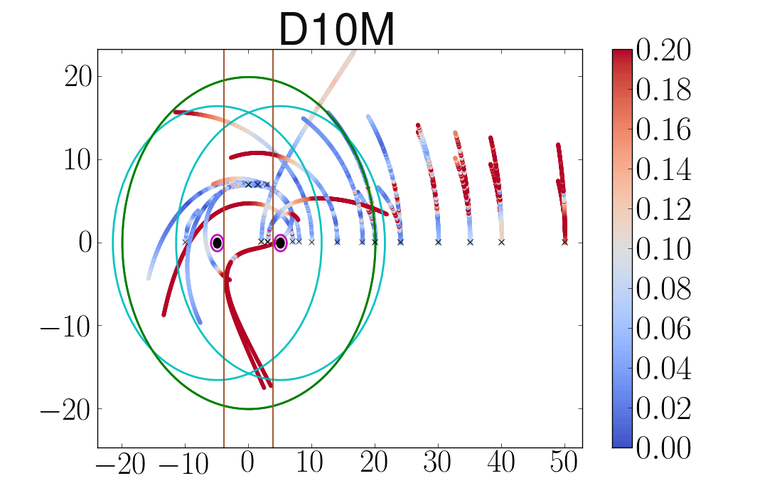
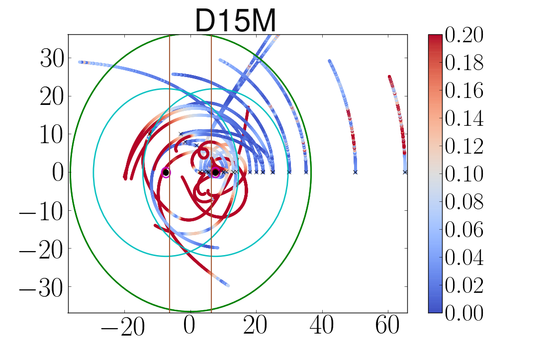
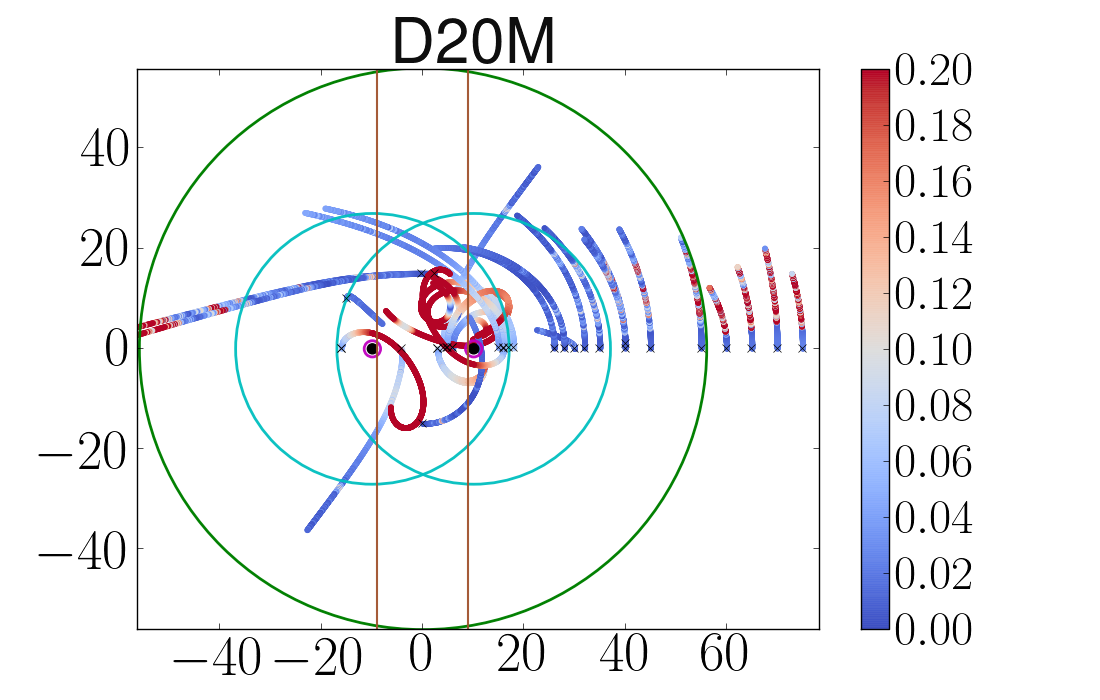
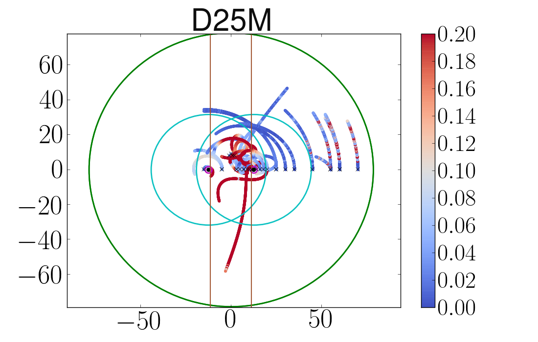
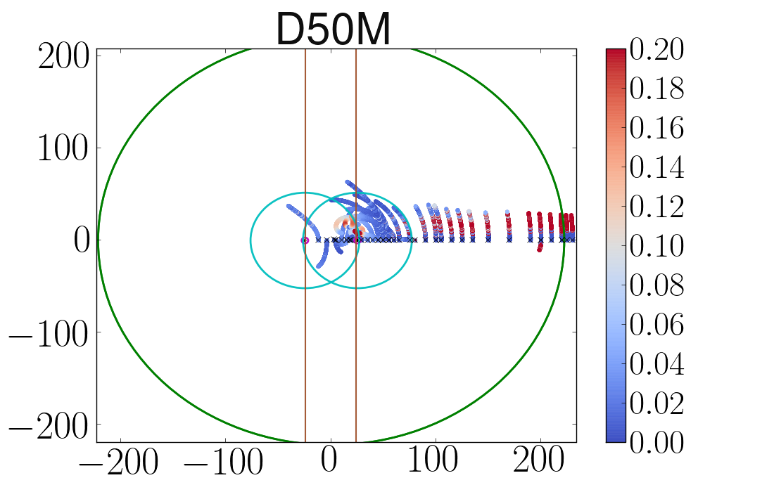
In Fig. 11, we show the relative difference between the curvature eigenvalues calculated using the numerical and analytic metrics. Here, we use a running average to smooth out the noise. Note that the color scale changes from blue to red at a 10% relative difference. From these plots, we can see that the buffer zone between the inner and near zones, as well as the near zone itself shows the smallest relative errors. The near-to-far zone buffer region (no plot shows the far zone) is generally worse, as least in terms of relative errors, than the near zone. The large relative differences seen for the $D=50M$ case may be due to noise, but as seen in Fig. 11, there are hints of systematic differences between the analytic and numerical spacetimes. Note that in Fig. 11, we plot the geodesics in a non-corotating frame. The reason for this is, that while plotting in a corotating frame allows us to see which zones the geodesics pass through, it also gives a false sense of how far in (quasi) inertial coordinates the geodesics actually traveled. By comparing the plots in Fig. 11 with Figs. 8–10, one can get a more accurate of the actual motion of each geodesic.

Figure 11: (Top two rows) A summary of the results. The plots show the trajectories of the geodesics in a non-corotating frame. The color scale gives the relative differences between the curvature eigenvalues (Sc) as calculated using the numerical (and smoothed by a running average) and analytic metrics. Note that the color changes from blues to reds at 10% relative difference. (Bottom two rows) Plots showing curvature eigenvalues as calculated using the analytical and numerical metrics, as well as a running average of the latter. There are hints here of systematic differences between the analytical and numerical results. However, as can be seen, the noise is much larger than these differences.

Figure 12: Curvature eigenvalues (Sc) for numerical and analytical spacetimes. For the analytical spacetime, we perturb the initial velocity of geodesics by the factors shown in the graphs. The dotted blue curve is the numerical result with velocity associated with the unperturbed analytic geodesic. As can be seen, the larger the value of the eigenvalues (i.e., geodesic deviation) the larger the effect of a $\pm 10\%$ perturbation. On the other hand, with small perturbations, we were able to find geodesics in the analytical spacetime that closely matched the dynamics (time dependence the eigenvalue) of the numerical one for geodesics farther than $r_{0}\sim 10M$ from the BHs.

IV.1 Comparing first and second-order matched spacetime

There are two versions of the analytic metric presented above. The standard one, known as the second-order metric, uses higher-order PN terms in the near zone, and matches the $\ell=2$ and $\ell=3$ multipoles in the inner zone. The first-order metric, which we will explore below, uses lower-order PN terms and only matches the $\ell=2$ multipoles in the inner zone.

Thus, we expect the second-order metric to be superior to the first-order one. In this section, we repeat our calculations comparing analytic metric to numerically evolved ones, but this time using the first-order analytic metric. Again, we plot results for $D=50M$, $D=20M$, $D=15M$, and $D=10M$ in Figs. 13, 14, 15, and 16. As in the sections above, we compare the curvature eigenvalues for from the analytic metric with the eigenvalues obtained by numerically evolving the analytic metric using the CCZ4 system. Thus we compare the second-order analytic eigenvalues with those obtained by numerically evolving the second-order metric and compare the first-order analytic eigenvalues with those obtained by numerically evolving the first-order metric. As expected, for $D\geq 15M$, the second-order curvature eigenvalues more closely match the associated numerical ones than the first-order eigenvalues do. For both metrics, the general trend for $D\geq 15M$ is that the first and second order results both become better at larger distances from the black holes and larger black-hole separations. The $D=10M$ results appear to be equally inaccurate for the first and second-order metrics. Our method is thus able to distinguish between a lower-accuracy and a higher-accuracy metric. Thus, we expect it will be a useful testing ground for developing still higher-accuracy analytic metrics.

Figure 13: A comparison of how well the curvature eigenvalues of the second-order metric and first-order metric agree with the eigenvalues of the associated numerical metrics for the $D=50M$ case. The top row shows the second-order results (which were previously shown in Fig. 8). The bottom row shows the first-order results. Note that at larger distances from the black holes the two results are comparable, while at closer distances the second-order results are qualitatively better.

Figure 14: A comparison of how well the curvature eigenvalues of the second-order metric and first-order metric agree with the eigenvalues of the associated numerical metrics for the $D=20M$ case. The top row shows the second-order results (which were previously shown in Fig. 9). The bottom row shows the first-order results. Unlike for the $D=50M$ case, there are significant differences between the analytical and numerical scalars for the first-order metric even at larger distances from the black holes.

Figure 15: A comparison of how well the curvature eigenvalues of the second-order metric and first-order metric agree with the eigenvalues of the associated numerical metrics for the $D=15M$ case. The top row shows the second-order results (which were previously shown in Fig. 10). The bottom row shows the first-order results. As with the $D=20M$ case, there are significant differences between the analytical and numerical scalars for the first-order metric even at larger distances from the black holes.

Figure 16: A comparison of how well the curvature eigenvalues of the second-order metric and first-order metric agree with the eigenvalues of the associated numerical metrics for the $D=10M$ case. The top row shows the second-order results (which were previously shown in Fig. 10). The bottom row shows the first-order results. Here, we do not see a significant improvement of the second-order metric over the first-order one.

V Discussion

In order to conclude if there are important systematic differences between the numerical and analytic metrics, we need to consider the possibility that the analytical metric is better approximated by an exact solution that does not agree exactly with the analytic metric on $\Sigma_{0}$. In such a case, one would expect that the appropriate initial conditions for the geodesics in the exact spacetime are not identical to those for the analytic one. But since small perturbations in the initial conditions of a geodesic can lead to significant differences on secular timescales (e.g., fall into one BH or the other, bounded versus unbounded, etc.), we considered here only geodesics that did not fall into the BHs or escape to large radii.

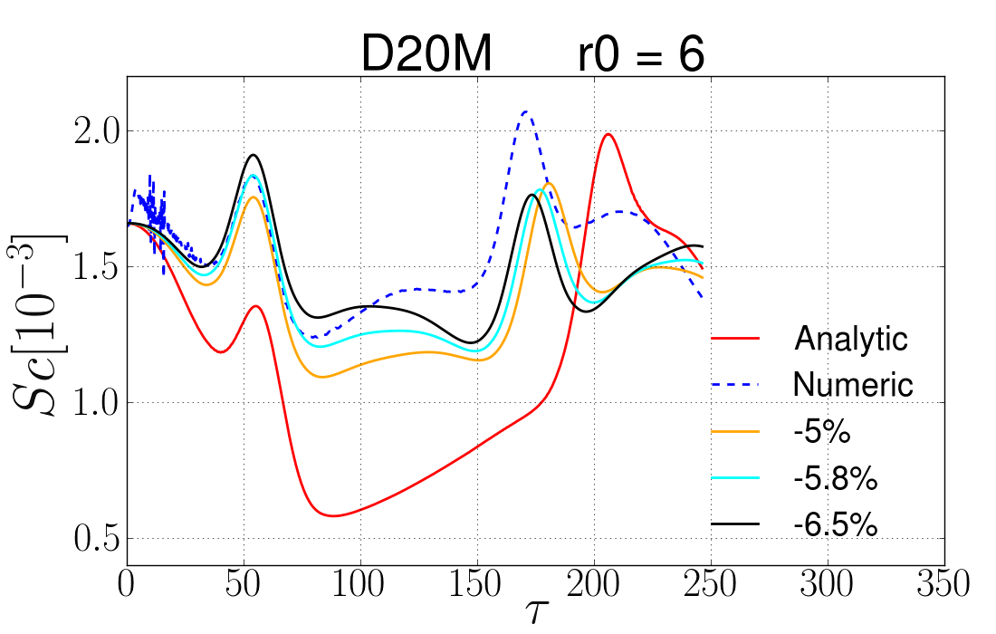
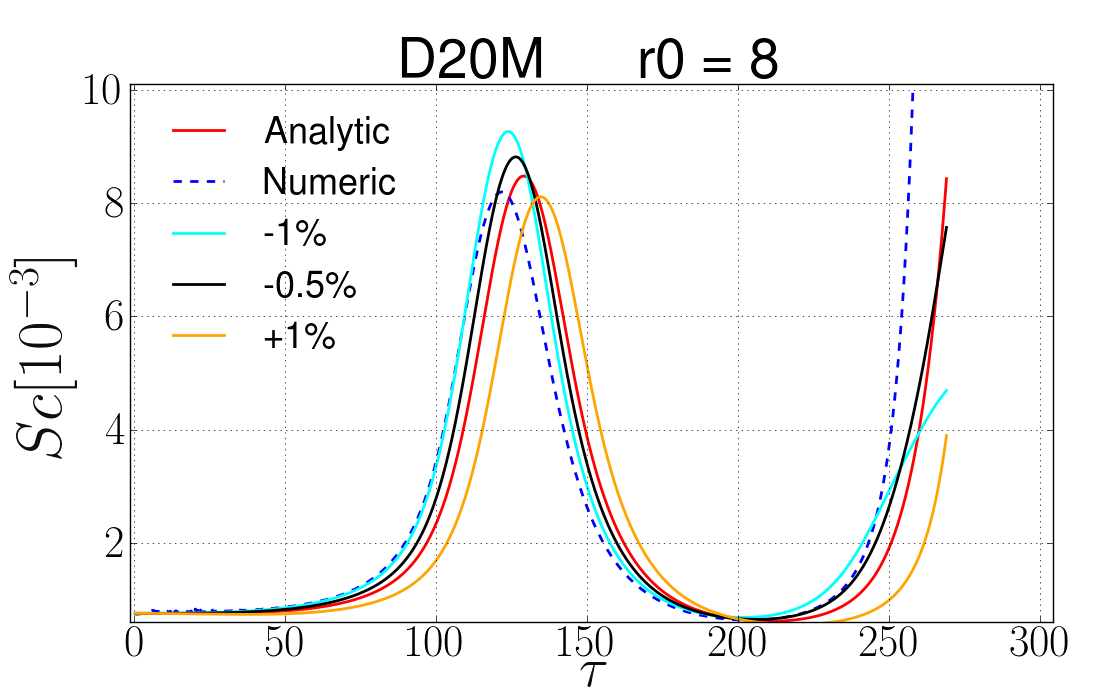
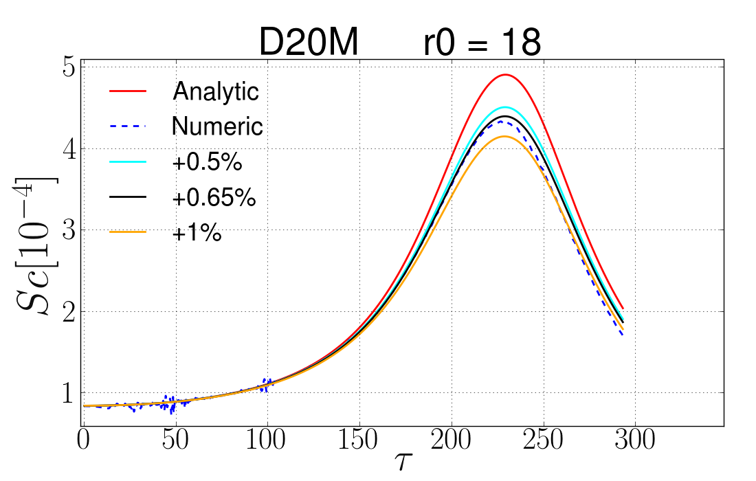
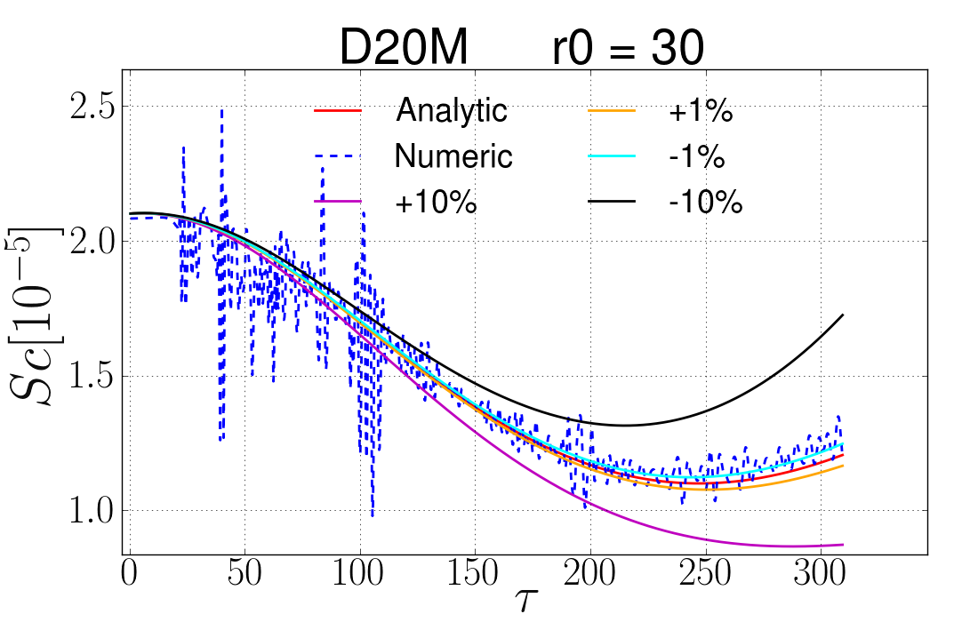
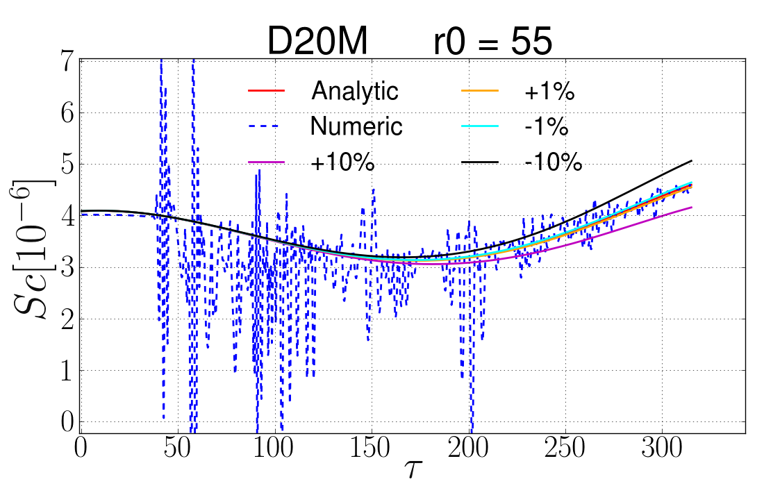
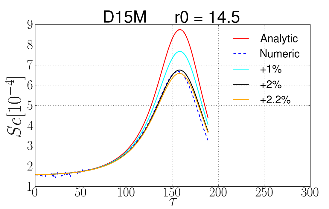
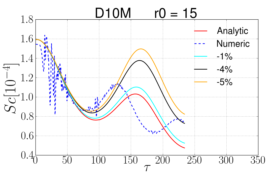
To see how small differences in the initial affect the geodesics we presented above (i.e., the stability of the above geodesics), we perturbed the initial velocities of a set of included geodesics by up to 10%. The results several geodesics are shown in Fig. 12 for the $D=20M$ case. We find that the effect of a $\sim 10\%$ perturbation is smaller for the farther out geodesics. We also find that a perturbation of $\lesssim 1\%$ seems to be sufficient to get reasonable agreement between the geodesics in the numerical and analytic spacetimes for geodesics farther than $r_{0}\sim 10M$ from the BHs. However, for the closer geodesic, the agreement is much poorer than for further out ones, which matches the general trend seen in Fig. 9. Indeed, for the $r_{0}=6M$ case, no perturbation is able to reproduce the behavior of the numerical geodesic past $\tau\sim 75M$. To further support the argument that small differences in the scalars can be removed by small changes on the initial conditions of the geodesics but large differences cannot be removed, we examined geodesics a distance of $\sim 15M$ from the black holes for the $D=15M$ and $D=10M$ case. Here we see that no perturbation of the $D=10M$ geodesic’s initial conditions will lead to qualitative agreement between the analytical and numerical eigenvalues. On the other hand, for the $D=15M$ very good agreement is achieved.

The fact that reasonable agreement between the analytical and numerical eigenvalues can be achieved by perturbing the analytical geodesics indicates a limitation of our basic method in that it may overemphasize the differences between to similar spacetimes. Large differences in the eigenvalues, like the ones seen in the $D=20M$ case near the BHs (and $D=10M$ everywhere) seem to be indicative of significant differences between the two spacetimes. On the other hand, where the differences are small, a given geodesic in one spacetime may behave nearly identically to one in the other, just with slightly different initial conditions. Consequently, one may expect that small differences in the eigenvalues will have little effect on, among others, gas dynamics.

One final note concerns the potential usefulness of our analysis at late times. The issue is that small differences in the trajectories generally grow on secular timescales. Thus the numerical and analytical eigenvalues represent curvature terms at increasingly different points of the spacetimes. For example, in the $D=25M$ case (see Fig. 9) for the farthest geodesics, we see differences between the numerical and analytic eigenvalues after about $\tau=400M$. From this point on, the geodesics will start taking different paths, and the scalars will disagree more and more, even though the two spacetimes are quite close, as is evident by the early time agreement of the scalars and the fact that the geodesics do not get significantly closer to either black hole. At close separations, these effects are larger and happen earlier. For example the $r_{0}=17.5M$ case shows significant deviations after $\tau=250M$, and the $r_{0}=9.5M$ shows significant differences after $\tau=75M$. The net effect is, the closer the two spacetimes are to each other (in the vicinity of the geodesic), the longer in time the analysis is valid.

VI Conclusion

In this paper, we introduced a new method for comparing the geodesic dynamics of two spacetimes. We used this method to compare the dynamics of recently developed analytical metrics that approximate the metric from an inspiraling black hole binary with fully nonlinear numerical evolutions of the Einstein equations. We find that the agreement in the dynamics between the two spacetimes is generally better for more separated binaries. Close to the black holes, as one might expect, we see the largest differences. Interestingly, we see that these differences scale in a highly nonlinear way with separation, with the $D=10M$ spacetime showing much larger differences than the $D=15M$ one. On the other hand, even for the $D=50M$ case, there are measurable differences in the geodesic deviation scalars between the analytical and numerical spacetimes for geodesics farther than $r_{0}\sim 100M$ from the black holes.