The CARMENES search for exoplanets around M dwarfs

Abstract

Context. The new CARMENES instrument comprises two high-resolution and high-stability spectrographs that are used to search for habitable planets around M dwarfs in the visible and near-infrared regime via the Doppler technique.

Aims. Characterising our target sample is important for constraining the physical properties of any planetary systems that are detected. The aim of this paper is to determine the fundamental stellar parameters of the CARMENES M-dwarf target sample from high-resolution spectra observed with CARMENES. We also include several M-dwarf spectra observed with other high-resolution spectrographs, that is CAFE, FEROS, and HRS, for completeness.

Methods. We used a $\chi^{2}$ method to derive the stellar parameters effective temperature $T_{\rm eff}$, surface gravity $\log{g}$, and metallicity [Fe/H] of the target stars by fitting the most recent version of the PHOENIX-ACES models to high-resolution spectroscopic data. These stellar atmosphere models incorporate a new equation of state to describe spectral features of low-temperature stellar atmospheres. Since $T_{\rm eff}$, $\log{g}$, and [Fe/H] show degeneracies, the surface gravity is determined independently using stellar evolutionary models.

Results. We derive the stellar parameters for a total of 300 stars. The fits achieve very good agreement between the PHOENIX models and observed spectra. We estimate that our method provides parameters with uncertainties of $\sigma_{T_{\rm eff}}=51$ K, $\sigma_{\log{g}}=0.07$, and $\sigma_{\rm[Fe/H]}=0.16$, and show that atmosphere models for low-mass stars have significantly improved in the last years. Our work also provides an independent test of the new PHOENIX-ACES models, and a comparison for other methods using low-resolution spectra. In particular, our effective temperatures agree well with literature values, while metallicities determined with our method exhibit a larger spread when compared to literature results.

1 Introduction

M dwarfs are of great interest for current exoplanet searches. Compared to Sun-like stars, M dwarfs have lower stellar masses and smaller radii, which facilitates detecting orbiting planets, especially those within the habitable zone (i.e. the orbital distance from the star at which liquid water can exist on the surface of the planet). Within this context, the Calar Alto high-Resolution search for M dwarfs with Exo-earths with Near-infrared and optical Échelle Spectrographs (CARMENES) instrument was built to search for rocky planets in the habitable zones of M dwarfs via the Doppler technique. CARMENES is mounted on the Zeiss 3.5 m telescope at Calar Alto Observatory, located in Almería, in southern Spain. After commissioning at the end of 2015 (see Quirrenbach et al., 2016), CARMENES has been taking data since January 1, 2016. The instrument consists of two fiber-fed spectrographs spanning the visible and near-infrared wavelength range, from 0.52 to 0.96 $\mu$m and from 0.96 to 1.71 $\mu$m, with a spectral resolution of R $\approx$ 94,600 and 80,500, respectively. Simultaneous observations in two wavelength ranges are favourable for distinguishing between a planetary signal and stellar activity, which can mimic a false-positive signal. Both spectrographs are designed to perform high-accuracy radial-velocity measurements with a long-term stability of $\sim$1 m s^-1 (Quirrenbach et al., 2014; Reiners et al., 2017), with the aim of being able to detect 2 M_⊕ planets orbiting in the habitable zone of M5 V stars.

To select the most promising targets, an extensive literature search was carried out (Alonso-Floriano et al., 2015; Caballero et al., 2016a). Additional observations were conducted with low- and high-resolution spectrographs and high-resolution imaging. A first paper about the CARMENES science preparation was published by Alonso-Floriano et al. (2015). They focused on the determination of spectral types and activity indices from low-resolution spectra and also gave a description of the CARMENES target sample. Cortés-Contreras et al. (2017) searched for close low-mass companions in the CARMENES target sample and analysed possible multiplicity using lucky imaging data. Jeffers et al. (2018) determined rotational velocities and H$\alpha$ activity indices measured from high-resolution spectra taken with CAFE and FEROS. The Carmencita database (CARMENes Cool dwarf Information and daTa Archive, Alonso-Floriano et al., 2015) contains all the information collected from the target sample, that is, astrometry; distances; spectral types; photometry in 20 different bands; X-ray count rates and hardness ratios; H$\alpha$ emission; rotational, radial, and Galactocentric velocities; stellar and planetary companionship; membership in open clusters and young moving groups; and targets in other radial-velocity surveys.

Because of their lower temperatures, M dwarfs show more complex spectra than Sun-like stars. Forests of spectral features caused by molecular lines make the determination of atmospheric parameters more difficult and require a full spectral synthesis. This necessitates the use of accurate atmosphere models that reproduce the spectral features present in cool star spectra. The PHOENIX-ACES models that we used here were presented by Husser et al. (2013).

It is important for planet search surveys to determine fundamental stellar parameters to be able to characterise the system. Gaidos & Mann (2014, hereafter GM14) observed $JHK$-band spectra of 121 M dwarfs. About half of them were also observed in the visible range. The authors determined effective temperatures in the visible by fitting BT-Settl models (Allard et al., 2012a) to their spectra. For stars without spectra in the visible, they calculated spectral curvature indices from $K$-band spectra to determine effective temperatures. They derived metallicities using the relation of the atomic line strength in the visible, $J,H,$ and $K$ bands as defined in Mann et al. (2013). The relations were calibrated using binaries with F, G, and K primary stars that have an M-dwarf companion. The BT-Settl models were also used by Rojas-Ayala et al. (2012, hereafter RA12), who determined temperatures and metallicities of 133 M dwarfs in the near-infrared $K$ band with mid-resolution TripleSpec spectra ($R\sim$ 2700). They measured the equivalent widths of Na i and Ca i and the H₂O-K2 index, quantifying the absorption due to H₂O opacity by using BT-Settl models (Allard et al., 2012a) with solar metallicity.

Rajpurohit et al. (2013) also used the models by Allard et al. (2012b) to calculate effective temperatures for 152 M dwarfs with low- and mid-resolution spectra. They found that the overall slope of model and observed spectra matched very well, although there were still some discrepancies in the depth of single lines and absorption bands.

Another widely used set of models are the MARCS models (Gustafsson et al., 2008). Among others, Lindgren & Heiter (2017) used these models together with the package Spectroscopy Made Easy (SME – Valenti & Piskunov, 1996) to determine metallicities for several M dwarfs from fitting several atomic species in the near-infrared. Souto et al. (2017) also fitted MARCS models to high-resolution APOGEE spectra to derive abundances for 13 elements of the exoplanet-hosting M dwarfs Kepler-138 and Kepler-186. Veyette et al. (2017) combined spectral synthesis, empirical calibrations, and equivalent widths to derive precise temperatures as well as Ti and Fe abundances from high-resolution M-dwarf spectra in the near-infrared. A more detailed overview of the different approaches on the determination of stellar parameters can be found in Passegger et al. (2016). In contrast to the above mentioned works, we here analyse a large sample of 300 M dwarfs by fitting high-resolution spectra to the most advanced model spectra using broad wavelength ranges. We obtain $T_{\rm eff}$, $\log{g}$, and [Fe/H] for all target stars from spectra taken with CARMENES, FEROS, CAFE, and HRS, compare our results with the literature, and show our conclusions.

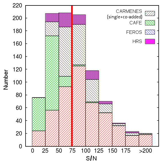
Figure 1: Histogram distribution of the signal-to-noise ratios for all spectra from all four spectrographs. The red solid line marks the signal-to-noise ratio limit of 75.

2 Observations

We obtained 973 spectra of 544 stars with spectral types between M0.0 V and M8.0 V with CARMENES and the high-resolution spectrographs CAFE, FEROS, and HRS. The Calar Alto Fiber-fed Echelle spectrograph (CAFE) is mounted at the 2.2 m telescope of the Calar Alto Observatory in Spain (Aceituno et al., 2013). The Fiber-fed Extended Range Optical Spectrograph (FEROS) spectrograph is an echelle spectrograph located at the 2.2 m telescope at the ESO La Silla Observatory in Chile (Kaufer et al., 1997; Stahl et al., 1999). The High Resolution Spectrograph (HRS) is an echelle spectrograph mounted at the 9.2 m Hobby-Eberly telescope at McDonald Observatory in Texas, USA (Tull et al., 1998). For a detailed description of the observations and the reduction process of CAFE, FEROS, and HRS data, we refer to Jeffers et al. (2018). The properties of the spectrographs and observations are summarised in Table 1. The CARMENES spectra were reduced automatically every night by the CARMENES pipeline (Caballero et al., 2016b). In our analysis we also used the co-added CARMENES spectra, which are produced by the SERVAL pipeline to measure radial-velocity shifts (Zechmeister et al., 2017; Reiners et al., 2017). For each star, the co-added spectrum consists of at least five single observations that are co-added to increase the signal-to-noise ratio (S/N).

We found that for most spectra with S/N¡75, the temperatures and metallicities were either unrealistically high or low, therefore we set a general S/N limit of 75 for all spectra. In order to examine spectra with the highest S/N, we first analysed all co-added CARMENES spectra, followed by single CARMENES spectra for stars without co-added spectra. We also investigated stars that are not being monitored by CARMENES for completeness, therefore we included spectra from FEROS, CAFE, and HRS in our analysis. When the same star was observed with more than one instrument, we selected the observation with higher S/N. Passegger (2017) showed that parameters derived from spectra from different spectrographs are comparable with deviations smaller than the typical uncertainty for these parameters. A histogram distribution showing the S/Ns for all spectra is presented in Fig. 1. After applying the S/N limit we finally determined parameters of 300 different M dwarfs, 235 of which were observed with CARMENES.

Table 1: Summary of observations and analysed stars.

Spectrograph	Resolution	$\Delta\lambda$ [nm]	Number of	Number of	Number of	Observing period
			spectra (observed)	stars (observed)	stars (results)
CARMENES	~94600	550-1700	485	338	235	2016-01-01 to 2017-06-30
CAFE	~62000	396-950	187	77	2	2013-01-21 to 2014-09-26
FEROS	48000	350-920	222	107	55	2012-12-31 to 2014-07-11
HRS	60000	420-1100	79	22	8	2011-09-29 to 2013-06-18
Total	…	…	973	544	300	…

Table 2: Wavelength regions and lines used for the $\chi^{2}$ fitting.

Line/band	$\gamma$-TiO	K i	Ti i	Fe i	Mg i
$\lambda_{c}$[nm]	705.5	770.1	841.5, 842.9, 843.7, 843.8	847.1, 851.6, 867.7	880.9
			846.9, 867.8, 868.5	869.1, 882.7

3 Method

We adapted the method described in Passegger et al. (2016), who determined the fundamental stellar parameters effective temperature $T_{\rm eff}$, surface gravity $\log{g}$, and metallicity [Fe/H] for four M dwarfs using the latest grid of PHOENIX model spectra presented by Husser et al. (2013). The PHOENIX code was developed by Hauschildt (1992, 1993) and has been considerably improved since then (e.g. Hauschildt et al. 1997; Hauschildt & Baron 1999; Claret et al. 2012; Husser et al. 2013). The code can generate 1D model atmospheres of plane-parallel or spherically symmetric stars and degenerate objects (late-type stars as well as brown dwarfs, white dwarfs, and giants), accretion discs, and expanding envelopes of novae and supernovae. Synthetic spectra can be calculated in 1D and 3D using local thermal equilibrium (LTE) or non-LTE radiative transfer for any desired spectral resolution.

This new PHOENIX-ACES model grid was especially designed for modelling spectra of cool dwarfs, because it uses a new equation of state to improve the calculations of molecule formation in cool stellar atmospheres. This allows good fitting of the $\gamma$- and $\epsilon$-TiO bands ($\lambda_{\rm head}$ 705 nm and $\lambda_{\rm head}$ 843 nm, respectively), which are very sensitive to effective temperature. The $\epsilon$-TiO band is especially sensitive to temperatures lower than 3000 K. The models use solar abundances from Asplund et al. (2009). Models with [$\alpha$/Fe] $\neq 0$ are only available for $T_{\rm eff}$ ¿ 3500 K and $3\leq$ [Fe/H] $\leq 0$. Therefore, we focus our analysis on models with [$\alpha$/Fe]=0. In this context, Veyette et al. (2016) reported a significant effect on the spectra of M dwarfs if abundances of other elements are varied. They found that a change in the C/O ratio influences the pseudo-continuum by changing TiO and H₂O opacities. In our study, however, we focused on the application of the latest PHOENIX-ACES models, with [Fe/H] being the only free abundance parameter.

We slightly modified the algorithm developed by Passegger et al. (2016). Because all stars in our sample have effective temperatures hotter than 3000 K, we only included the $\gamma$-TiO band in our fitting. Passegger et al. (2016) also showed that the K i and Na i doublets around 768 nm and 819 nm, respectively, are suitable for surface gravity and metallicity determination. Since the K i line at 766.5 nm is contaminated by telluric lines, we decided to exclude it from the fitting. We excluded the Ca ii doublet at 850.0 nm and 866.4 nm as well, because these lines are not well reproduced by the models: they are formed in the chromosphere and can show emission when the star is magnetically active. The Na i doublet around 819 nm was previously used because of its high pressure sensitivity (see Passegger et al., 2016). In a detailed analysis of the first results of our large sample, we found a degeneracy in the strength and width of the Na i doublet over a wide parameter range, which made it difficult to distinguish between a cool-metal poor and a hot-metal rich model. Therefore we excluded this doublet from our analysis. The $\gamma$-TiO band and Mg i line ($\lambda$ 880.9 nm) were found to be more suitable for metallicity determination, and they were therefore assigned higher weights during fitting. As an example, Fig. 2 presents $\chi^{2}$ maps of the Mg i line for one of our stars in the $T_{\rm eff}$-$\log{g}$ and $T_{\rm eff}$-[Fe/H] plane, where a strong dependency on metallicity can be seen. A $\chi^{2}$ minimisation is used to determine the best fit of the models to the observed spectra. As described in Passegger et al. (2016), the procedure is divided into two steps, which are described in the following.

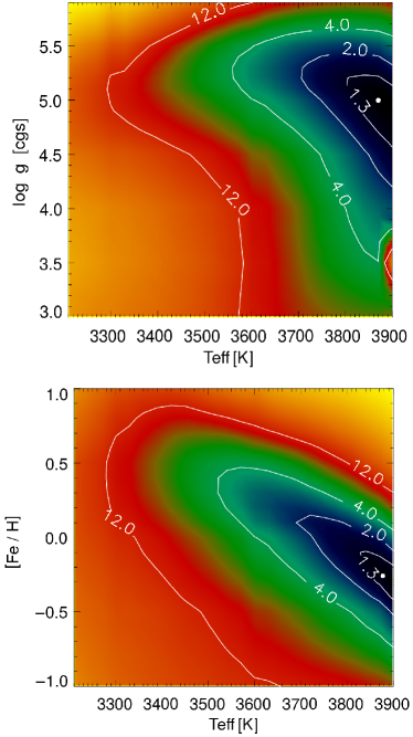
Figure 2: $\chi^{2}$ map of the Mg i line for BR Psc (GJ 908) with $\chi^{2}$ contour values. The upper panel shows the $T_{\rm eff}$-$\log{g}$ plane, and the lower panel the $T_{\rm eff}$-[Fe/H] plane. The minimum for this line is indicated with a white dot.

3.1 Coarse grid search

In a first step, we used the coarsely spaced grid of the model spectra in a wide range around the expected parameters of the star. To match the instrumental resolutions, the model spectra were first convolved with a Gaussian. Then the average flux of the models and the observed spectrum was normalised to unity by assuming a pseudo-continuum for each wavelength range. Next, the models were interpolated to match the wavelength grid of the observed spectrum, so that each wavelength point of each model spectrum could be compared to the stellar spectrum. The value of $\chi^{2}$ was calculated to find a rough global minimum. This was done for different wavelength ranges between 705.0 and 820.5 nm. The parameters for the three best minima were given as an output in order to provide different starting values for the downhill simplex in the next step.

3.2 Fine grid search

In the second step, the region around each global minimum was explored on a finer grid. The wavelength range was extended to 883.5 nm to include some titanium and iron lines. An overview of all regions and lines used for fitting is presented in Table 2. To reduce the number of free parameters in the fit, we used the values of projected rotation velocity $v\sin{i}$ determined by Jeffers et al. (2018) using cross-correlation. To account for $v\sin{i}$, the model spectra were broadened using a broadening function. The function determined the effect on the line spread function caused by stellar rotation. The resulting line spread function was convolved with the model spectrum. In contrast to Passegger et al. (2016), who used the IDL curvefit function, we used a downhill simplex method for fitting, which we found to be more robust on large samples. The downhill simplex used linear interpolation between the model grid points to explore the parameter space in detail. A $\chi^{2}$ minimisation finds the best-fit model. This was done for all three minima found in the previous step. The parameters with the best $\chi^{2}$ were selected as results.

From the first results for our sample, the fits showed very good agreement between models and observed spectra. However, we found that the values of $\log{g}$ and [Fe/H] were much higher than expected for main-sequence M dwarfs; the $\log{g}$ was between 5.5 and 6.0, and most metallicities were super-solar, with values of up to 1.0 dex. Moreover, we found exceptionally low $\log{g}$ of 3.0 with metallicities of $-1.0$ dex for some stars. In both cases the fitted models agreed very well with the data. The results of obviously wrong parameter values can be explained by a degeneracy between $T_{\rm eff}$, $\log{g}$, and [Fe/H], which is displayed in Fig. 3. Especially the $T_{\rm eff}$-[Fe/H] map shows a largely extended minimum. To break this degeneracy, we decided to determine $\log{g}$ using an independent method.

Figure 3: $\chi^{2}$ maps for BR Psc (GJ 908) for different combinations of stellar parameters. The global minimum is indicated with a white dot.

Baraffe et al. (1998) presented evolutionary models for low-mass stars up to 1.4 M_⊙. A new version of these models was published by Baraffe et al. (2015) using updated solar abundances. However, the Baraffe et al. (1998) and Baraffe et al. (2015) $T_{\rm eff}$-$\log{g}$ relations are consistent with each other in the temperature range of M dwarfs, therefore we used the Baraffe et al. (1998) version. Amongst other parameters, they provided effective temperatures and surface gravities for different stellar ages and metallicities of 0.0 and $-$0.5 dex. Unfortunately, the ages of the stars in the CARMENES target sample are not yet well constrained. This will be the topic of upcoming papers. A preliminary kinematics and activity analysis of the sample to qualitatively estimate ages was carried out by Cortés-Contreras (2016). Therefore, we assumed an age of 5 Gyr for the whole sample. This seems to be a good guess even for younger stars because once M dwarfs reach the main sequence they evolve extremely slowly (e.g. Burrows et al., 1997; Laughlin et al., 1997). This is also reflected in the Baraffe et al. (1998) relations, which agree within 0.02 dex in $\log{g}$ for ages between 1 and 7 Gyr in the temperature range of M dwarfs up to 4000 K. In the algorithm the downhill simplex can vary $T_{\rm eff}$ and metallicity. Based on this, $\log{g}$ was determined from the $T_{\rm eff}$-$\log{g}$ relations. Metallicities between 0.0 and $-$0.5 dex were linearly interpolated from the relations to estimate $\log{g}$. For metallicities higher than 0.0 dex or lower than $-$0.5 dex, the values were extrapolated. Because the differences in $\log{g}$ depending on metallicity are small (no larger than 0.20 dex between metallicities 0.0 and $-$0.5 dex), we expect the uncertainty from the interpolation and extrapolation to be negligible compared to the uncertainty coming from the fitting. From these three parameters, the corresponding PHOENIX model was interpolated and the $\chi^{2}$ was calculated. Fig. 4 shows a co-added CARMENES spectrum of a typical M1 V star with the best-fit model, including the lines and regions we used for fitting.

Figure 4: Co-added CARMENES spectrum of the M1 V star GX And (black) and the best-fit model (blue: whole fit, and red: regions used for $\chi^{2}$ minimisation).

4 Results and discussion

Table A.1 presents the fundamental parameters of our target sample. It includes the CARMENES identifiers, spectral types from Carmencita, $T_{\rm eff}$, $\log{g}$, and [Fe/H] derived in this study, $v\sin{i}$ determined by Jeffers et al. (2018), masses from Carmencita (see section 4.4), a flag for Ca ii emission, and the instrument with which the analysed spectrum was observed. We applied the method for error estimation as given in Passegger et al. (2016). They estimated errors by adding Poisson noise to 1400 model spectra with random parameter distributions to simulate S/N $\sim$ 100 and applied their algorithm to recover the input parameters. Using this method, we derived uncertainties of 51 K for $T_{\rm eff}$, 0.07 dex for $\log{g}$, and 0.16 dex for [Fe/H], which are consistent with typical uncertainties in literature. We confirmed this statement by calculating deviations between our results and literature values ($\sigma_{\rm exp}$) together with the corresponding standard deviation ($\sigma_{\Delta}$). The numbers are presented in Table 3, showing that $\sigma_{\Delta}$ are smaller than the expected deviations $\sigma_{\rm exp}$ for the different literature samples.

Table 3: Expected errors and deviations in $T_{\rm eff}$, $\log{g}$, and [Fe/H] of our results and the literature.

Authora	$T_{\rm eff}$ [K]		$\log{g}$ [dex]		[Fe/H] [dex]
	$\sigma_{\rm{exp}}$	$\sigma_{\Delta}$	$\sigma_{\rm{exp}}$	$\sigma_{\Delta}$	$\sigma_{\rm{exp}}$	$\sigma_{\Delta}$
RA12	63	108	…	…	0.23	0.19
GM14	93	78	…	…	0.18	0.13
Ma15	85	51	0.09	0.08	0.18	0.10
a RA12: Rojas-Ayala et al. (2012), GM14: Gaidos & Mann (2014),
Ma15: Maldonado et al. (2015).

4.1 Effective temperature

The histogram distributions for all parameters for all 300 stars are presented in Fig. 5. The temperature distribution (left panel) shows that most of the stars in our sample have temperatures of between 3200 K and 3800 K, corresponding to spectral types ranging from M0.0 V to M5.0 V. Figure 6 gives a comparison of 98 stars that overlap with the samples of RA12, Maldonado et al. (2015, hereafter Ma15), and GM14. Ma15 determined effective temperature and metallicity from optical spectra using pseudo-equivalent widths. In general, most of our results agree with the literature values within the error bars. However, there is one group of outliers at the cool end of the sample. This group is represented by results from RA12, who determined temperatures using the H₂O-K2 index calibrated with BT-Settl models of solar metallicity. They derived temperatures that are cooler than ours by about 200 K. Two more outliers are located around 3550 K (GJ 752A) and 3650 K (BR Psc/GJ 908), for which RA12 determined considerably hotter temperatures of 3789 and 3995 K, respectively. However, our temperatures are consistent with those derived by Ma15 and GM14, which makes the result of RA12 discrepant. A small “bump” can be found between 3550 and 3700 K, where GM14 tended to derive slightly higher temperatures than we do. For other stars in Fig. 6, the values are mostly consistent with our results.

4.2 Surface gravity

The middle panel of Fig. 5 presents the $\log{g}$ distribution for our sample. Ma15 determined $\log{g}$ for early-M dwarfs using stellar masses from photometric relations and radii from an empirical mass-radius relation that combines interferometry (von Braun et al., 2014; Boyajian et al., 2012) and data from low-mass eclipsing binaries (Hartman et al., 2015). A comparison of those stars that we have in common is presented in the middle panel of Fig. 6. The grey lines indicate a 1 $\sigma$ deviation of 0.07 dex. We calculated $\log{g}$ for the sample of GM14 from the provided masses and radii. The uncertainties were derived with error propagation from the uncertainties in mass and radius. We included $\log{g}$ values based on interferometric radius measurements from Boyajian et al. (2012). We derived the $\log{g}$ in the same way as for GM14. Our results are consistent with the $\log{g}$ values from Ma15, which mostly lie between 4.6 and 5.0 dex. Most of the interferometrically based $\log{g}$ also agree with our values. This is expected since they are constrained by the $T_{\rm eff}$-$\log{g}$ relations. It also shows consistency between the empirical radius calibration of Ma15 and theoretical models. However, when we compare our $\log{g}$ values with those of GM14, we find some offset. At the lower end of the plot, we derive higher values than GM14. Because $\log{g}$ depends on $T_{\rm eff}$ in our calculation, this trend is consistent with the bump found in the temperature plot. The values of Boyajian et al. (2012) slightly follow the same trend as GM14, although the sample is too small to draw a definite conclusion.

4.3 Metallicity

The right panel of Fig. 5 displays the metallicity distribution of our results, centred on solar metallicity. The right panel of Fig. 6 shows a comparison of the stars that we have in common with RA12, Ma15, and GM14. Their metallicity measurements range from –0.6 to 0.4 dex, whereas our results only range from –0.4 to almost 0.2 dex. This indicates that the metallicity is more difficult to constrain than the other parameters, and that different methods could give noticeably different results. On the other hand, we find that even for spectra for which the parameters agree with the literature, some lines, such as Ti i ($\lambda$ 846.9 nm and 867.77 nm) and Fe i ($\lambda$ 867.71 nm and 882.6 nm), are too deep. A possible explanation might be the contrast between the line and the continuum so that the models still cannot reproduce the correct line depths. On the other hand, we used models with element abundances fixed to solar. A change in [$\alpha$/Fe] or [Ti/Fe] might improve the fit for some stars. A more extensive study on the performance of the models themselves, probably including different element abundances, is necessary to completely understand their behaviour.

4.4 Relation of spectral type, mass, and temperature

We present the relation between stellar mass and effective temperature in Fig. 7, and the metallicities are colour-coded. The thick black line represents the theoretical relation from Baraffe et al. (1998) for an age of 5 Gyr and solar metallicity. The masses were calculated by combining mass-luminosity relations from Delfosse et al. (2000, for 4.5 mag ¡ Ks ¡ 5.29 mag) and Benedict et al. (2016, for 5.29 mag ¡ Ks ¡ 10 mag), with the magnitudes taken from the Carmencita database (see Alonso-Floriano et al., 2015). In this plot, stars with super-solar metallicity should lie below the relation reported by Baraffe et al. (1998) and stars with sub-solar metallicity should lie above this relation. As can be seen, most of the stars lie below the theoretical prediction. This can be due to several reasons: our $T_{\rm eff}$s are systematically underestimated, our metallicities are slightly lower than expected, or the determined stellar masses are overestimated. Based on the literature comparison in Section 4.1, we can exclude the former two. Since Delfosse et al. (2000) did not provide errors for their mass-luminosity relation, we assumed an average uncertainty of 10% in mass over the whole mass range, which is of the same order as the errors from Benedict et al. (2016). Within this range, our values agree with the theoretical relation of Baraffe et al. (1998). Some obvious outliers are identified by numbers and are discussed in more detail later.

Figure 8 shows the effective temperatures of all stars as a function of their spectral type; the spectral types are taken from the Carmencita database. The green stars show the expected temperature-spectral type relation as presented by Kenyon & Hartmann (1995). The authors computed effective temperatures, colours, spectral types, and bolometric corrections for main-sequence stars from B0 to M6 after an extensive literature search. Their temperatures fit our results for solar metallicities well. The large spread in temperature for each spectral type is caused by different metallicities, which are colour-coded. This indicates that stars of the same spectral type have higher temperatures if they are more metal-rich, or in other words: for the same effective temperature, the spectral type decreases with increasing metallicity. This can be explained with an increase in opacity in the optical with increasing metallicity, mainly dominated by TiO and VO molecular bands. The peak of the energy distribution is therefore shifted towards longer wavelengths and makes the star appear redder, that is, of later spectral type. This effect has been discussed in more detail by Delfosse et al. (2000); Chabrier & Baraffe (2000). A similar trend was found by Mann et al. (2015), who derived empirical relations between $T_{\rm eff}$, [Fe/H], radii, and luminosities. They showed that the radius increases with metallicity for a fixed temperature (see their Figure 23).

Figure 5: Histogram distributions of $T_{\rm eff}$ (left panel) together with spectral types from Kenyon & Hartmann (1995) on the upper x-axis, $\log{g}$ (middle panel), and [Fe/H] (right panel) for our 300 stars.

Figure 6: Comparison between values from our sample and literature values for $T_{\rm eff}$ (left panel), $\log{g}$ (middle panel), and [Fe/H] (right panel). The black line indicates the 1:1 relation. The grey lines indicate the 1$\sigma$ deviation of 51 K, 0.07 dex in $\log{g}$, and 0.16 dex in [Fe/H]. The black dots with error bars in the lower right corner of each plot show the uncertainties of this work.

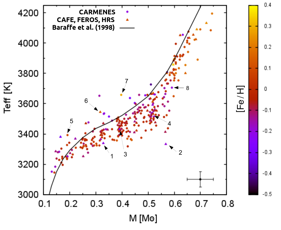
Figure 7: Effective temperature as a function of stellar mass. The determined metallicities of the stars are colour-coded. The different symbols present stars observed with CARMENES or CAFE, FEROS, and HRS. The thick black line shows the theoretical relation for solar metallicity from Baraffe et al. (1998). An average uncertainty of 10% in mass is indicated by the black dot with error bars in the lower right corner. The eight outliers discussed in Section 4.5 are labelled.

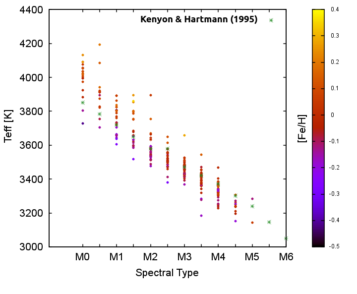
Figure 8: Effective temperature as a function of spectral type. The determined metallicities of the stars are colour-coded. The green stars indicate the expected temperatures for each spectral type computed by Kenyon & Hartmann (1995).

4.5 Analysis of outliers

In the following, eight outliers found in the mass-temperature plot of Fig. 7 are discussed in more detail. We selected them because their $T_{\rm eff}$ or metallicity clearly deviate from the relation reported by Baraffe et al. (1998).

1: J03430+459.

This star was observed with HRS. The best-fit model agrees moderately well with the observed spectrum, with small deviations in the TiO bandheads and some Ti i and Fe i lines. Alonso-Floriano et al. (2015) measured a pseudo-equivalent width of –0.7 Å for H$\alpha$. Newton et al. (2017) also reported that this star is slightly active. This could explain the deviations in the Fe i and Ti i lines, which are sensitive to magnetic Zeeman splitting. A change in [Ti/Fe] or [$\alpha$/Fe], on the other hand, could also be responsible for a deviation in the fit of Ti i lines.

2: J04544+650.

For this star we also used HRS spectra to determine the parameters. The star is magnetically active, has an H$\alpha$ pseudo-equivalent width of –13.9 Å (Alonso-Floriano et al., 2015), and shows Ca ii emission. We find deviations in some Ti i and Fe i lines, which could explain the deviation in metallicity.

3: J05078+179.

This star was observed with FEROS. The best spectrum has an S/N of 104. The star shows H$\alpha$ emission with a pseudo-equivalent width of –0.7 Å (Jeffers et al., 2018). The activity also causes distortion in other lines (e.g. some Fe i and Ti i lines). Here, the deviations in some Ti i lines might also be caused by Ti abundances that are different from solar, and this might in turn explain the low metallicity.

4: J11201-104.

We analysed CARMENES spectra of this star and found it to be too metal-poor in the mass-$T_{\rm eff}$ plot. The star has strong Ca ii emission. Alonso-Floriano et al. (2015) reported an H$\alpha$ pseudo-equivalent width of –3.3 Å. The magnetic activity might explain the deviations in the Fe i lines here as well, and therefore also the deviation in the determined lower metallicity.

5: J18346+401.

For this star we used a co-added CARMENES spectrum to derive the parameters. The best model fits the observed spectrum very well. The resulting temperature of 3391 K is comparable to the temperature measured by Gaidos & Mann (2014) from near-infrared data. However, Gaidos & Mann (2014) determined a metallicity of 0.42 dex, whereas we obtained a more metal-poor value of 0.09 dex. The line depth is well fitted in our spectrum. We also derived a lower $\chi^{2}$ compared to the parameter set of Gaidos & Mann (2014). The star is not known to be active and does not show any Ca ii emission either. Considering all this information, we cannot explain the measured low metallicity satisfactorily.

6: J21057+502.

We analysed HRS spectra for this star and found good agreement between the observed spectra and the best-fit models. Our derived temperature of 3543 K is about 100 K too hot for the spectral type M3.5. However, the $\chi^{2}$-map shows a large extended minimum in the $T_{\rm eff}$-$\log{g}$-[Fe/H] planes, which reaches from almost 3700 K and +0.5 [Fe/H] down to 3500 K and +0.1 [Fe/H], making the derived parameters less significant. Cortés-Contreras (2016) reported from an analysis of the stellar kinematics that this star is part of the young disc and a probable member of the local association, which is 10-150 Myr old. The models of Baraffe et al. (1998) show that using an age of 5 Gyr for a star younger than 0.5 Gyr can lead to an increase in $T_{\rm eff}$ of 50–100 K. Accounting for these two circumstances results in a slightly lower temperature and metallicity, which causes the star to fit the mass-$T_{\rm eff}$ relation better.

7: J21152+257.

The fit to this co-added CARMENES spectrum is good: we find only minor deviations between observed and fitted lines, especially for the TiO-band. The star is inactive and does not show any signs of emission in H$\alpha$ or Ca ii. The determined temperature of 3657 K is about 200 K hotter than expected for the stated spectral type M3. The $\chi^{2}$-map has a large extended and deep minimum here as well, which is located between about 3800 K and +0.5 [Fe/H], and 3550 K and +0.1 [Fe/H]. This might explain the too high temperature and metallicity.

8: J21221+229.

The parameters of this star were also derived from a co-added CARMENES spectrum, for which the model fit is very good. The star is not active, and the spectral type M1 corresponds to the fitted temperature of 3704 K. We are unable to explain the deviation in Fig. 7 for this star.

5 Summary

CARMENES is a new instrument at the Calar Alto observatory that simultaneously takes high-resolution spectra in the visible and near-infrared wavelength ranges. Its aim is to search for Earth-sized planets in the habitable zone around M dwarfs.

We provided precise parameters from PHOENIX-ACES model fits for effective temperature, surface gravity, and metallicity for 300 M dwarfs, which is the largest sample of M dwarfs investigated with high-resolution spectroscopy so far. It is important not only for CARMENES, but also for future exoplanet surveys, since knowing stellar fundamental parameters is essential for characterising an orbiting planet. Moreover, accurate metallicities are crucial for theories of planet formation around low-mass stars and give information on the chemical evolution of the Galaxy.

Our work presents a test of the new PHOENIX-ACES models on a large sample of low-mass stars and points out inconsistencies in line depths and metallicity determination. This analysis also serves as a comparison of methods using low- and high-resolution spectra for stellar parameter determination. Table 4 summarises the different literature approaches for determining stellar parameters. It illustrates that in contrast to other comparable studies, we used high-resolution spectra and fitting of the latest model atmospheres. Comparisons with literature values for some of the target stars showed that we achieve very good agreement in the temperatures. For the metallicity we find an overall distribution that shows mainly sub-solar values and peaks between 0.0 and $-$0.1 dex, which agrees with findings from Gaidos & Mann (2014, see their Figure 1). Our values are consistent with the literature within 1 $\sigma$, although there is no obvious correlation between our values and literature results. This might indicate an inconsistency in metallicity determination as such and may require further improvement of methods and models. Simultaneous fitting of all three parameters did not provide reliable results for all sample stars. Therefore, we determined $\log{g}$ from temperature- and metallicity-dependent relations from evolutionary models assuming an average age of 5 Gyr for our sample. However, we showed that our results in $\log{g}$ agree well with interferometric observations by Boyajian et al. (2012), which also serves as an evaluation of theoretical evolutionary models and observations.

To confirm our results, we performed $\chi^{2}$ fits with our spectra and models with parameters determined by GM14, Ma15, and RA12. We compared the $\chi^{2}$s with those resulting from fits with our derived parameters and found the smallest $\chi^{2}$ for 92% of the fits with our parameters. For the remaining 8%, the literature parameters agree with ours within their errors. This confirms that our method, using the latest PHOENIX-ACES models, provides the best-fit parameters to our observations. It shows that our method has the potential to derive accurate stellar parameters for M dwarfs. This contributes to the most extensive catalogue of M-dwarf parameters so far. However, we also showed that there are still some shortcomings in synthetic models for low-temperature atmospheres, although they have significantly improved in the past decade. While the PHOENIX-ACES models fit observed spectra very well and show only negligible deviations within the noise level, we can find some discrepancies. From the fit, the full line depth is not represented for some lines, which might be the reason for the differences in metallicity we found compared to literature values. A small offset in metallicity is also depicted in Fig. 7. Our results for solar metallicity lie systematically below the mass-luminosity relation of Baraffe et al. (1998), but largely follow the theoretical prediction. Further detailed analysis of the models is necessary for better understanding the metallicity dependency.

We identified eight outliers; four of them show activity either in H$\alpha$ or Ca ii. Magnetic activity can distort line profiles by Zeeman splitting (e.g. Hébrard et al., 2014; Reiners et al., 2013), which could explain deviations in some sensitive Fe i and Ti i lines. Furthermore, a Ti and $\alpha$-element abundance different from the Sun might also cause deviations in the Ti i lines. Two outliers are caused by large extended and deep minima in the $T_{\rm eff}$-$\log{g}$-[Fe/H] planes. One of these stars is believed to have an age younger than 0.5 Gyr (Cortés-Contreras, 2016), which results in a too high temperature when using the models of Baraffe et al. (1998) for 5 Gyr. For two outliers we were not able to provide any explanation.

Finally, an accurate age determination of the sample stars would be helpful. This topic will be addressed in subsequent CARMENES papers. The S/N also has a significant influence on the parameter determination, which makes a high S/N preferable when using the method we presented here. A great advantage of the new CARMENES instrument is its capability to provide simultaneous observations in the visible and near-infrared wavelength range. A detailed investigation of spectra in both ranges is desirable to better understand M-dwarf atmospheres. The analysis of CARMENES near-infrared spectra will be presented in forthcoming works.

Table 4: Summary of literature approaches for the stellar parameter determination.

Authora	Resolution	$\Delta\lambda$ [nm]	$T_{\rm eff}$	$\log{g}$	[Fe/H]
RA12	~2700	1000-2400	H2O-K2 index	…	Na i and Ca i EW,
					H2O-K2 index
GM14	800 to 1000	320-970	BT-Settl fit,	…	atomic line
	2000	800-2400	spec. curvature		strength relation
Ma15	115,000	378-693	pseudo-EW	masses and radii	pseudo-EW
				from empirical relation
This work	48000 to	700-880	PHOENIX-ACES fit	Baraffe et al. (1998)	PHOENIX-ACES fit
	94600		with downhill simplex	relation	with downhill simplex
a RA12: Rojas-Ayala et al. (2012), GM14: Gaidos & Mann (2014), Ma15: Maldonado et al. (2015).

Appendix A Table of parameters

The online version contains full names and equatorial coordinates of all stars. The electronic form is available at the CDS via anonymous ftp to cdsarc.u-strasbg.fr (130.79.128.5) or via http://cdsweb.u-strasbg.fr/cgi-bin/qcat?J/A+A/.
Columns and references to $v\sin i$ are discussed in a footnote below the table.

[x]llcccccll
Basic astrophysical parameters of investigated stars^a.
Karmn Spectral $T_{\rm eff}$ [K] $\log{g}$ [dex] [Fe/H] [dex] $v\sin i$ M Ca ii IRT Instrument
type ($\pm$ 51 K) ($\pm$ 0.07 dex) ($\pm$ 0.16 dex) [km/s] [M_⊙] emission
Basic astrophysical parameters of investigated stars^a (cont.).
Karmn Spectral $T_{\rm eff}$ [K] $\log{g}$ [dex] [Fe/H] [dex] $v\sin i$ M Ca ii IRT Instrument
type ($\pm$ 51 K) ($\pm$ 0.07 dex) ($\pm$ 0.16 dex) [km/s] [M_⊙] emission
J00051+457 M1.0 V 3665 4.85 –0.16 ¡ 3 0.565 … CARM co-add
J00056+458 M0.0 V 4055 4.64 +0.11 ¡ 3 0.672 … CAFE
J00162+198E M4.0 V 3336 5.02 0.08 ¡ 3 0.302 … CARM co-add
J00183+440 M1.0 V 3606 4.93 –0.27 2.5^b 0.449 … CARM co-add
J00184+440 M3.5 V 3283 5.11 –0.19 1.9^c 0.159 … CARM co-add
J00286–066 M4.0 V 3387 4.99 0.05 ¡ 3 0.385 … CARM co-add
J00315–058 M3.5 V 3392 5.01 –0.02 ¡ 3 0.323 … FEROS
J00389+306 M2.5 V 3537 4.89 –0.04 2.5^b 0.472 … CARM co-add
J00395+149S M4.0 V 3334 5.06 –0.09 ¡ 3 0.332 … HRS
J00570+450 M3.0 V 3425 4.99 –0.05 ¡ 3 0.394 … CARM co-add
J01013+613 M2.0 V 3537 4.92 –0.13 4.0^d 0.442 … CARM co-add
J01025+716 M3.0 V 3478 4.92 0.00 2.5^b 0.512 … CARM co-add
J01026+623 M1.5 V 3796 4.69 0.13 ¡ 3 0.597 yes CARM co-add
J01125–169 M4.5 V 3152 5.17 –0.20 2.5^b 0.132 … CARM co-add
J01339–176 M4.0 V 3335 5.07 –0.11 ¡ 3 0.254 … CARM co-add
J01384+006 M2.0 V 3644 4.80 0.01 ¡ 3 0.532 … FEROS
J01433+043 M2.0 V 3534 4.91 –0.08 2.5^b 0.451 … CARM co-add
J01518+644 M2.5 V 3553 4.89 –0.06 4.0^d 0.467 … CARM co-add
J02002+130 M3.5 V 3185 5.15 –0.18 ¡ 3 0.144 … CARM co-add
J02015+637 M3.0 V 3495 4.93 –0.05 2.5^b 0.521 … CARM co-add
J02026+105 M4.5 V 3254 5.12 –0.17 6.00 0.191 yes FEROS
J02050–176 M2.5 V 3534 4.88 0.00 ¡ 3 0.519 … FEROS
J02070+496 M3.5 V 3414 5.02 –0.12 ¡ 3 0.431 … CARM co-add
J02096–143 M2.5 V 3555 4.87 0.00 ¡ 3 0.533 … FEROS
J02116+185 M3.0 V 3428 4.97 0.00 ¡ 3 0.385 … FEROS
J02123+035 M1.5 V 3659 4.81 –0.05 ¡ 3 0.497 … CARM co-add
J02222+478 M0.5 V 3921 4.68 0.06 4 0.622 … CARM co-add
J02336+249 M4.0 V 3293 5.09 –0.11 3.1 0.208 yes CARM co-add
J02358+202 M2.0 V 3595 4.88 –0.10 ¡ 3 0.555 … CARM co-add
J02362+068 M4.0 V 3326 5.03 0.04 ¡ 3 0.261 … CARM co-add
J02442+255 M3.0 V 3459 4.96 –0.07 2.5^b 0.384 … CARM co-add
J02565+554W M1.0 V 3891 4.66 0.19 4.0^d 0.689 … CARM co-add
J02581–128 M2.5 V 3381 5.08 –0.30 ¡ 3 0.165 … FEROS
J03026–181 M2.5 V 3613 4.78 0.12 ¡ 3 0.517 … FEROS
J03181+382 M1.5 V 3854 4.66 0.20 2.5^c 0.642 … CARM co-add
J03213+799 M2.0 V 3574 4.90 –0.11 4.0^d 0.465 … CARM co-add
J03217–066 M2.0 V 3552 4.91 –0.13 ¡ 3 0.521 yes CARM co-add
J03233+116 M2.5 V 3412 5.02 –0.11 ¡ 3 0.447 yes FEROS
J03430+459 M4.0 V 3338 5.08 –0.20 ¡ 3 0.329 … HRS
J03438+166 M0.0 V 4034 4.64 0.12 ¡ 3 0.657 … FEROS
J03463+262 M0.0 V 3997 4.65 0.11 ¡ 3 0.658 yes CARM co-add
J03531+625 M3.0 V 3484 4.94 –0.04 ¡ 3 0.380 … CARM co-add
J04225+105 M3.5 V 3438 4.96 0.00 ¡ 3 0.575 … CARM co-add
J04290+219 M0.5 V 4194 4.59 0.20 1.11^e 0.744 … CARM co-add
J04311+589 M4.0 V 3325 5.03 0.05 ¡ 3 0.313 … CARM co-add
J04376–110 M1.5 V 3624 4.84 –0.05 ¡ 3 0.520 … CARM co-add
J04376+528 M0.0 V 4034 4.68 –0.09 ¡ 3 0.653 yes CARM co-add
J04429+189 M2.0 V 3582 4.88 –0.08 ¡ 3 0.537 … CARM co-add
J04429+214 M3.5 V 3424 4.98 0.00 ¡ 3 0.323 … CARM co-add
J04520+064 M3.5 V 3391 5.00 0.00 2.5^b 0.400 … CARM co-add
J04538–177 M2.0 V 3563 4.90 –0.12 2.5^b 0.460 … CARM
J04544+650 M4.0 V 3332 5.09 –0.19 ¡ 3 0.568 yes HRS
J04588+498 M0.0 V 4015 4.65 0.09 ¡ 3 0.649 yes CARM co-add
J05033–173 M3.0 V 3416 5.01 –0.10 2.5^b 0.288 … CARM
J05050+442 M5.0 V 3285 5.10 –0.12 ¡ 3 0.146 … HRS
J05078+179 M3.0 V 3432 5.02 –0.20 3 0.391 … FEROS
J05091+154 M3.0 V 3412 5.01 –0.09 4 0.565 yes FEROS
J05127+196 M2.0 V 3579 4.89 –0.12 2.5^b 0.491 … CARM co-add
J05280+096 M3.5 V 3362 5.03 –0.03 ¡ 3 0.249 … CARM co-add
J05298–034 M2.5 V 3474 4.93 0.00 ¡ 3 0.455 … FEROS
J05314–036 M1.5 V 3894 4.64 0.25 ¡ 3^f 0.599 … CARM co-add
J05348+138 M3.5 V 3424 4.98 0.00 2.5^b 0.405 … CARM co-add
J05360–076 M4.0 V 3365 5.01 0.01 4.0^d 0.259 … CARM co-add
J05365+113 M0.0 V 4075 4.65 0.04 6.40 0.655 yes CARM co-add
J05366+112 M4.0 V 3333 5.07 –0.14 ¡ 3 0.283 yes CARM
J05415+534 M1.0 V 3863 4.69 0.08 2.0^c 0.605 … CARM co-add
J05421+124 M4.0 V 3310 5.05 0.04 ¡ 3 0.223 … CARM co-add
J05532+242 M1.5 V 3755 4.71 0.11 ¡ 3 0.616 … CARM co-add
J06011+595 M3.5 V 3358 5.02 0.00 ¡ 3 0.265 … CARM co-add
J06103+821 M2.0 V 3543 4.89 –0.05 2.5^b 0.458 … CARM co-add
J06105–218 M0.5 V 3822 4.71 0.06 1.0^f 0.598 … CARM co-add
J06246+234 M4.0 V 3238 5.11 –0.08 ¡ 3 0.150 … CARM co-add
J06277+093 M2.0 V 3534 4.92 –0.12 ¡ 3 0.513 … FEROS
J06325+641 M4.0 V 3469 4.94 –0.01 ¡ 3 0.261 … HRS
J06371+175 M0.0 V 3728 4.89 –0.42 ¡ 3 0.510 … CARM co-add
J06396–210 M4.0 V 3322 5.06 –0.04 3.70 0.253 … CARM
J06421+035 M3.5 V 3436 4.96 0.02 ¡ 3 0.419 … CARM
J06548+332 M3.0 V 3450 4.96 –0.02 ¡ 3 0.392 … CARM co-add
J07033+346 M4.0 V 3276 5.10 –0.12 3.50 0.270 yes CARM co-add
J07044+682 M3.0 V 3469 4.94 –0.01 ¡ 3 0.418 … CARM co-add
J07081–228 M2.0 V 3664 4.79 –0.01 ¡ 3 0.512 … FEROS
J07274+052 M3.5 V 3358 5.01 0.04 ¡ 3 0.315 … CARM co-add
J07287–032 M3.0 V 3458 4.95 –0.02 2.5^b 0.447 … CARM co-add
J07319+362N M3.5 V 3319 5.06 –0.03 ¡ 3 0.422 yes CARM co-add
J07349+147 M3.0 V 3435 5.00 –0.09 4.8 0.398 yes FEROS
J07353+548 M2.0 V 3526 4.93 –0.14 ¡ 3 0.415 … CARM co-add
J07361–031 M1.0 V 3891 4.69 0.05 3.5 0.621 yes CARM co-add
J07386–212 M3.0 V 3417 5.00 –0.09 ¡ 3 0.319 … CARM co-add
J07393+021 M0.0 V 4005 4.66 0.07 ¡ 3 0.650 yes CARM co-add
J07545+085 M2.5 V 3483 4.96 –0.13 ¡ 3 0.448 … FEROS
J07582+413 M3.5 V 3363 5.02 0.00 ¡ 3 0.262 … CARM co-add
J08126–215 M4.0 V 3326 5.03 0.04 ¡ 3 0.189 … CARM
J08161+013 M2.0 V 3589 4.86 –0.06 ¡ 3 0.500 … CARM co-add
J08293+039 M2.5 V 3575 4.88 –0.07 ¡ 3 0.470 … CARM
J08313–060 M1.5 V 3802 4.68 0.16 ¡ 3 0.642 … FEROS
J08344–011 M3.5 V 3371 5.02 –0.03 ¡ 3 0.250 … FEROS
J08358+680 M2.5 V 3471 4.95 –0.06 ¡ 3 0.399 … CARM
J08371+151 M2.5 V 3489 4.92 0.00 ¡ 3 0.507 … FEROS
J08402+314 M3.5 V 3381 5.02 –0.04 ¡ 3 0.295 … CARM
J08427+095 M0.0 V 4024 4.64 0.14 ¡ 3 0.682 … FEROS
J08428+095 M2.5 V 3505 4.91 –0.01 ¡ 3 0.430 … FEROS
J08526+283 M4.5 V 3307 5.03 0.13 2.5^b 0.248 … CARM
J08551+015 M0.0 V 4091 4.61 0.25 ¡ 3 0.686 … FEROS
J09008+052E M3.5 V 3457 4.94 0.02 ¡ 3 0.414 … FEROS
J09008+052W M3.0 V 3424 4.97 0.05 ¡ 3 0.455 … FEROS
J09023+084 M2.5 V 3507 4.90 0.00 ¡ 3 0.521 … FEROS
J09028+680 M4.0 V 3343 5.03 0.01 4.0^d 0.244 … CARM
J09133+688 M2.5 V 3545 4.93 –0.16 ¡ 3 0.462 yes CARM
J09143+526 M0.0 V 4053 4.65 0.07 ¡ 3 0.622 … CAFE
J09144+526 M0.0 V 3994 4.68 –0.03 3.21^g 0.605 yes CARM co-add
J09163–186 M1.5 V 3584 4.90 –0.14 ¡ 3 0.563 … CARM
J09288–073 M2.5 V 3496 4.91 0.00 ¡ 3 0.385 … FEROS
J09307+003 M3.5 V 3413 4.99 –0.01 ¡ 3 0.319 … CARM
J09360–216 M2.5 V 3488 4.96 –0.14 2.5^b 0.362 … CARM
J09411+132 M1.5 V 3601 4.88 –0.14 ¡ 3 0.519 … CARM co-add
J09423+559 M3.5 V 3384 4.99 0.07 ¡ 3 0.425 … CARM
J09425+700 M2.0 V 3511 4.91 –0.03 10.0^h 0.560 yes CARM co-add
J09428+700 M3.0 V 3423 4.99 –0.04 2.5^b 0.491 … CARM co-add
J09468+760 M1.5 V 3683 4.78 0.00 ¡ 3 0.568 … CARM co-add
J09511–123 M0.5 V 3753 4.77 –0.09 ¡ 3 0.585 … CARM co-add
J09561+627 M0.0 V 3974 4.67 0.07 ¡ 3 0.640 yes CARM co-add
J10023+480 M1.0 V 3768 4.73 0.03 ¡ 3 0.601 … CARM co-add
J10087+027 M3.0 V 3486 4.90 0.06 ¡ 3 0.392 … FEROS
J10122–037 M1.5 V 3613 4.87 –0.12 ¡ 3 0.575 … CARM co-add
J10125+570 M3.5 V 3408 4.99 –0.01 ¡ 3 0.321 … CARM
J10158+174 M3.5 V 3392 5.01 –0.02 ¡ 3 0.319 … FEROS
J10167–119 M3.0 V 3511 4.89 0.01 ¡ 3 0.534 … CARM co-add
J10243+119 M2.0 V 3488 4.95 –0.10 ¡ 3 0.511 … FEROS
J10251–102 M1.0 V 3761 4.73 0.05 ¡ 3 0.569 … CARM co-add
J10289+008 M2.0 V 3575 4.89 –0.09 ¡ 3 0.485 … CARM co-add
J10350–094 M3.0 V 3457 4.95 –0.03 ¡ 3 0.397 … CARM
J10354+694 M3.5 V 3418 4.98 –0.01 ¡ 3 0.388 … CARM co-add
J10396–069 M2.5 V 3524 4.91 –0.06 ¡ 3 0.541 … CARM
J10416+376 M4.5 V 3263 5.07 0.05 4.1^j 0.212 … CARM
J10508+068 M4.0 V 3335 5.03 0.03 ¡ 3 0.281 … CARM co-add
J10520+139 M3.5 V 3372 5.02 –0.03 ¡ 3 0.289 … FEROS
J11000+228 M2.5 V 3500 4.94 –0.10 2.5^b 0.423 … CARM co-add
J11026+219 M1.0 V 3896 4.69 0.04 4.5 0.603 yes CARM co-add
J11033+359 M1.5 V 3598 4.87 –0.09 ¡ 3 0.452 … CARM co-add
J11054+435 M1.0 V 3636 4.91 –0.29 ¡ 3 0.430 … CARM co-add
J11110+304 M2.0 V 3753 4.70 0.14 ¡ 3 0.599 … CARM co-add
J11126+189 M1.5 V 3752 4.73 0.06 ¡ 3 0.565 … CARM co-add
J11201–104 M2.0 V 3540 4.97 –0.27 ¡ 3 0.515 yes CARM
J11289+101 M3.5 V 3364 5.02 0.00 ¡ 3 0.363 … CARM
J11306–080 M3.5 V 3419 4.98 –0.01 ¡ 3 0.390 … CARM
J11417+427 M4.0 V 3358 4.99 0.13 ¡ 3 0.381 … CARM co-add
J11421+267 M2.5 V 3512 4.90 –0.02 ¡ 3 0.485 … CARM co-add
J11467–140 M3.0 V 3523 4.87 0.06 ¡ 3 0.570 … CARM
J11476+786 M3.5 V 3359 5.02 0.00 ¡ 3 0.258 … CARM co-add
J11477+008 M4.0 V 3251 5.10 –0.04 ¡ 3 0.172 … CARM co-add
J11509+483 M4.5 V 3211 5.11 0.00 ¡ 3 0.168 … CARM co-add
J11511+352 M1.5 V 3633 4.88 –0.18 ¡ 3 0.506 … CARM co-add
J11532–073 M2.5 V 3555 4.87 0.00 ¡ 3 0.498 … FEROS
J12016–122 M3.0 V 3509 4.88 0.04 ¡ 3 0.386 … FEROS
J12054+695 M4.0 V 3325 5.02 0.09 ¡ 3 0.293 … CARM co-add
J12100–150 M3.5 V 3365 4.99 0.12 ¡ 3 0.433 … CARM co-add
J12111–199 M3.0 V 3448 4.97 –0.06 3.0^d 0.391 … CARM
J12123+544S M0.0 V 3923 4.70 –0.01 3.9 0.635 … CARM co-add
J12230+640 M3.0 V 3528 4.87 0.03 ¡ 3 0.529 … CARM co-add
J12248–182 M2.0 V 3476 4.98 –0.18 ¡ 3 0.271 … CARM
J12312+086 M0.5 V 3913 4.71 –0.05 ¡ 3 0.611 … CARM co-add
J12350+098 M2.5 V 3578 4.85 0.00 ¡ 3 0.524 … CARM
J12388+116 M3.0 V 3429 4.96 0.04 ¡ 3 0.513 … CARM co-add
J12428+418 M4.0 V 3321 5.07 –0.10 3 0.289 … CARM co-add
J12479+097 M3.5 V 3384 5.00 0.06 ¡ 3 0.354 … CARM co-add
J13196+333 M1.5 V 3801 4.67 0.18 ¡ 3 0.606 … CARM co-add
J13209+342 M1.0 V 3732 4.76 –0.01 ¡ 3 0.576 … CARM co-add
J13229+244 M4.0 V 3318 5.05 0.02 ¡ 3 0.264 … CARM co-add
J13293+114 M3.5 V 3431 4.96 0.04 ¡ 3 0.394 … CARM
J13299+102 M0.5 V 3704 4.82 –0.15 ¡ 3 0.562 … CARM co-add
J13343+046 M0.0 V 4131 4.60 0.24 4 0.723 … FEROS
J13427+332 M3.5 V 3359 5.03 –0.01 4.0^d 0.285 … CARM co-add
J13450+176 M1.0 V 3806 4.85 –0.42 2.0^k 0.572 … CARM co-add
J13457+148 M1.5 V 3677 4.79 –0.04 ¡ 3 0.539 … CARM co-add
J13458–179 M3.5 V 3399 4.99 0.04 ¡ 3 0.333 … CARM
J13526+144 M2.0 V 3670 4.74 0.13 ¡ 3 0.519 … FEROS
J14010–026 M1.0 V 3719 4.77 –0.03 ¡ 3 0.552 … CARM co-add
J14082+805 M1.0 V 3835 4.67 0.17 ¡ 3 0.618 … CARM co-add
J14152+450 M3.0 V 3456 4.94 0.00 ¡ 3 0.463 … CARM co-add
J14251+518 M2.5 V 3512 4.92 –0.08 ¡ 3 0.449 … CARM co-add
J14257+236E M0.5 V 3943 4.65 0.16 ¡ 3 0.653 … CARM co-add
J14257+236W M0.0 V 4021 4.63 0.18 ¡ 3 0.678 … CARM co-add
J14283+053 M3.0 V 3455 4.96 –0.03 ¡ 3 0.398 … FEROS
J14294+155 M2.0 V 3633 4.81 0.00 ¡ 3 0.555 … CARM co-add
J14307–086 M0.5 V 4084 4.63 0.13 ¡ 3 0.739 … CARM co-add
J14342–125 M4.0 V 3325 5.02 0.11 ¡ 3 0.303 … CARM co-add
J14524+123 M2.0 V 3560 4.88 –0.05 ¡ 3 0.516 … CARM co-add
J14544+355 M3.5 V 3375 5.00 0.03 ¡ 3 0.474 … CARM co-add
J15013+055 M3.0 V 3413 5.00 –0.04 ¡ 3 0.400 … CARM
J15095+031 M3.0 V 3480 4.93 –0.01 ¡ 3 0.482 … CARM co-add
J15194–077 M3.0 V 3430 5.00 –0.09 ¡ 3 0.330 … CARM co-add
J15412+759 M3.0 V 3430 5.02 –0.18 ¡ 3 0.339 … CARM co-add
J15474–108 M2.0 V 3515 4.96 –0.21 ¡ 3 0.523 … CARM
J15598–082 M1.0 V 3644 4.86 –0.15 ¡ 3 0.560 … CARM co-add
J16028+205 M4.0 V 3310 5.05 0.02 ¡ 3 0.249 … CARM co-add
J16092+093 M3.0 V 3455 4.98 –0.09 ¡ 3 0.390 … CARM co-add
J16120+033 M2.0 V 3592 4.91 –0.18 ¡ 3 0.518 … FEROS
J16167+672N M3.0 V 3504 4.91 0.00 ¡ 3 0.510 … CARM co-add
J16167+672S M0.0 V 4091 4.62 0.16 ¡ 3 0.699 … CARM co-add
J16254+543 M1.5 V 3516 4.98 –0.27 ¡ 3 0.350 … CARM co-add
J16303–126 M3.5 V 3378 5.01 0.01 ¡ 3 0.323 … CARM co-add
J16327+126 M3.0 V 3486 4.92 0.00 ¡ 3 0.390 … CARM co-add
J16462+164 M2.5 V 3505 4.92 –0.05 ¡ 3 0.484 … CARM co-add
J16487–157 M1.0 V 3805 4.68 0.16 ¡ 3 0.584 … FEROS
J16554–083N M3.5 V 3343 5.05 –0.04 2.7^m 0.198 … CARM co-add
J16578+473 M1.5 V 4300 4.68 –0.43 ¡ 3 0.705 … CARM co-add
J16581+257 M1.0 V 3734 4.78 –0.08 ¡ 3 0.572 … CARM co-add
J16591+209 M3.5 V 3364 5.06 –0.15 5.70 0.318 yes FEROS
J17033+514 M4.5 V 3237 5.08 0.06 ¡ 3 0.171 … CARM co-add
J17052–050 M1.5 V 3631 4.82 –0.01 ¡ 3 0.526 … CARM co-add
J17071+215 M3.0 V 3482 4.94 –0.05 ¡ 3 0.417 … CARM co-add
J17115+384 M3.5 V 3415 4.99 –0.01 ¡ 3 0.417 … CARM co-add
J17160+110 M1.0 V 3801 4.69 0.13 ¡ 3 0.570 … FEROS
J17166+080 M2.0 V 3544 4.91 –0.10 ¡ 3 0.449 … CARM co-add
J17198+417 M2.5 V 3499 4.93 –0.08 ¡ 3 0.409 … CARM co-add
J17303+055 M0.0 V 3804 4.77 –0.14 3.3 0.590 … CARM co-add
J17355+616 M0.5 V 3874 4.69 0.06 3.2 0.606 yes CARM co-add
J17378+185 M1.0 V 3654 4.88 –0.22 3 0.489 … CARM co-add
J17530+169 M3.0 V 3392 5.02 –0.08 ¡ 3 0.388 … FEROS
J17578+046 M3.5 V 3278 5.10 –0.12 ¡ 3 0.155 … CARM co-add
J17578+465 M2.5 V 3459 4.94 0.00 ¡ 3 0.447 … CARM co-add
J18051–030 M1.0 V 3664 4.87 –0.21 1.6^c 0.521 … CARM co-add
J18163+015 M3.0 V 3429 5.00 –0.10 ¡ 3 0.346 … FEROS
J18174+483 M2.0 V 3515 4.96 –0.18 ¡ 3 0.510 yes CARM co-add
J18180+387E M3.0 V 3434 4.99 –0.06 ¡ 3 0.295 … CARM co-add
J18198–019 K7.0 V 4133 4.66 –0.08 ¡ 3 - … CARM
J18221+063 M4.0 V 3405 5.00 0.00 ¡ 3 0.260 … CARM co-add
J18224+620 M4.0 V 3227 5.10 –0.01 2.3^m 0.159 … CARM co-add
J18240+016 M2.0 V 3514 4.93 –0.11 ¡ 3 0.508 … FEROS
J18312+068 M1.0 V 3804 4.71 0.06 ¡ 3 0.593 … FEROS
J18319+406 M3.5 V 3423 4.99 –0.05 ¡ 3 0.325 … CARM co-add
J18346+401 M3.5 V 3392 4.98 0.09 2.5^b 0.192 … CARM co-add
J18353+457 M0.5 V 3915 4.69 0.05 1.0ⁿ 0.631 … CARM co-add
J18363+136 M4.0 V 3301 5.07 –0.05 ¡ 3 0.266 … CARM co-add
J18409–133 M1.0 V 3788 4.72 0.06 3.0^c 0.583 … CARM co-add
J18419+318 M3.0 V 3473 4.95 –0.06 2.5^b 0.411 … CARM co-add
J18427+139 M4.0 V 3254 5.11 –0.11 ¡ 3 0.251 yes FEROS
J18480–145 M2.5 V 3500 4.94 –0.09 ¡ 3 0.453 … CARM co-add
J18518+165 M0.0 V 3884 4.71 –0.02 ¡ 3 0.598 … FEROS
J18580+059 M0.5 V 3913 4.68 0.08 ¡ 3 0.622 … CARM co-add
J19032+034 M3.0 V 3473 4.95 –0.07 ¡ 3 0.389 … FEROS
J19070+208 M2.0 V 3532 4.95 –0.21 ¡ 3 0.330 … CARM co-add
J19072+208 M2.0 V 3535 4.94 –0.20 ¡ 3 0.331 … CARM co-add
J19084+322 M3.0 V 3439 4.97 –0.04 ¡ 3 0.389 … CARM co-add
J19098+176 M4.5 V 3240 5.08 0.06 ¡ 3 0.190 … CARM co-add
J19169+051N M2.5 V 3557 4.86 0.00 ¡ 3 0.526 … CARM co-add
J19216+208 M4.5 V 3249 5.09 0.02 3.5 0.187 … CARM co-add
J19220+070 M3.0 V 3369 5.05 –0.16 ¡ 3 0.221 … FEROS
J19251+283 M3.0 V 3405 5.00 0.00 ¡ 3 0.398 … CARM co-add
J19346+045 M0.0 V 4054 4.69 –0.20 3.3 0.632 … CARM co-add
J20011+002 M2.0 V 3562 4.91 –0.13 ¡ 3 0.525 … FEROS
J20187+158 M2.5 V 3514 4.91 –0.04 ¡ 3 0.449 … FEROS
J20305+654 M2.5 V 3475 4.96 –0.08 ¡ 3 0.415 … CARM co-add
J20336+617 M4.0 V 3368 4.98 0.14 ¡ 3 0.420 … CARM co-add
J20405+154 M4.5 V 3236 5.09 0.03 ¡ 3 0.189 … CARM co-add
J20407+199 M2.5 V 3475 4.96 –0.07 ¡ 3 0.528 … FEROS
J20450+444 M1.5 V 3591 4.89 –0.14 ¡ 3 0.480 … CARM co-add
J20525–169 M4.0 V 3313 5.06 –0.01 ¡ 3 0.242 … CARM co-add
J20533+621 M0.5 V 3828 4.71 0.03 ¡ 3 0.597 … CARM co-add
J20556–140N M4.0 V 3372 5.02 0.01 ¡ 3 0.334 … CARM co-add
J20567–104 M2.5 V 3523 4.89 0.00 ¡ 3 0.502 … CARM co-add
J21019–063 M2.5 V 3521 4.90 –0.05 ¡ 3 0.513 … CARM co-add
J21057+502 M3.5 V 3543 4.83 0.14 ¡ 3 0.317 … HRS
J21127–073 M3.5 V 3471 4.96 –0.07 ¡ 3 0.328 … HRS
J21152+257 M3.0 V 3657 4.69 0.28 ¡ 3 0.397 … CARM co-add
J21164+025 M3.0 V 3475 4.95 –0.05 ¡ 3 0.402 … CARM co-add
J21221+229 M1.0 V 3705 4.83 –0.19 3.7 0.590 … CARM co-add
J21348+515 M3.0 V 3484 4.92 0.00 ¡ 3 0.494 … CARM co-add
J21463+382 M4.0 V 3304 5.06 –0.01 ¡ 3 0.168 … CARM co-add
J21466–001 M4.0 V 3346 5.02 0.05 4.0^d 0.292 … CARM co-add
J21466+668 M4.0 V 3355 5.01 0.05 ¡ 3 0.258 … CARM co-add
J21472–047 M4.5 V 3273 5.10 –0.11 ¡ 3 0.201 … HRS
J21574+081 M1.5 V 3858 4.62 0.34 ¡ 3 0.596 … FEROS
J22020–194 M3.5 V 3431 4.97 –0.01 ¡ 3 0.362 … CARM co-add
J22021+014 M0.5 V 3914 4.69 0.05 ¡ 3 0.600 … CARM co-add
J22057+656 M1.5 V 3653 4.85 –0.15 3.9 0.314 … CARM co-add
J22096–046 M3.5 V 3454 4.96 –0.01 ¡ 3 0.531 … CARM co-add
J22115+184 M2.0 V 3554 4.90 –0.10 ¡ 3 0.580 … CARM co-add
J22125+085 M3.0 V 3500 4.92 –0.04 ¡ 3 0.381 … CARM co-add
J22231–176 M4.5 V 3196 5.12 –0.05 ¡ 3 0.173 … CARM co-add
J22252+594 M4.0 V 3383 5.00 0.05 ¡ 3 0.385 … CARM co-add
J22298+414 M4.0 V 3318 5.03 0.10 ¡ 3 0.254 … CARM co-add
J22330+093 M1.0 V 3660 4.87 –0.22 2.64^c 0.525 … CARM co-add
J22503–070 M0.5 V 3895 4.73 –0.10 ¡ 3 0.600 … CARM co-add
J22532–142 M4.0 V 3359 5.01 0.06 2.5^b 0.370 … CARM co-add
J22559+178 M1.0 V 3824 4.70 0.07 ¡ 3 0.599 … CARM co-add
J22565+165 M1.5 V 3787 4.70 0.10 2.5^b 0.601 … CARM co-add
J23113+085 M3.5 V 3404 4.99 0.01 ¡ 3 0.330 … CARM co-add
J23175+063 M3.0 V 3481 4.93 –0.01 ¡ 3 0.400 … FEROS
J23216+172 M4.0 V 3361 4.99 0.14 ¡ 3 0.437 … CARM co-add
J23234+155 M2.0 V 3635 4.81 0.00 ¡ 3 0.509 … FEROS
J23245+578 M1.0 V 3824 4.69 0.12 0.5^c 0.606 … CARM co-add
J23340+001 M2.5 V 3553 4.87 0.00 ¡ 3 0.476 … CARM co-add
J23381–162 M2.0 V 3545 4.92 –0.13 ¡ 3 0.508 … CARM co-add
J23419+441 M5.0 V 3144 5.13 0.05 1.2^j 0.141 … CARM co-add
J23431+365 M4.0 V 3247 5.10 –0.05 2.6^m 0.208 … CARM co-add
J23492+024 M1.0 V 3657 4.84 –0.12 ¡ 3 0.465 … CARM co-add
J23556–061 M2.5 V 3648 4.76 0.11 ¡ 3 0.598 … CARM co-add
J23577+233 M3.5 V 3419 4.98 0.00 5.20 0.423 … FEROS
J23585+076 M3.0 V 3470 4.94 0.00 ¡ 3 0.507 … CARM co-add

^aCarmencita identifier (Karmn), spectral type, effective temperature, surface gravity, metallicity, $v\sin i$, mass, Ca ii emission flag, and instrument with which the spectrum was obtained (CARMENES –“CARM co-add” for co-added, “CARM” for single spectra), CAFE, FEROS, HRS). Rotational velocities ($v\sin i$) from Jeffers et al. (2018), if no other reference is given
^b Browning et al. (2010), ^c Houdebine (2010), ^d Reiners et al. (2012), ^e Martínez-Arnáiz et al. (2010), ^f Reiners & Basri (2007), ^g Antonova et al. (2013), ^h Stauffer & Hartmann (1986), ^j Jenkins et al. (2009), ^k Glebocki & Gnacinski (2005), ^m Mohanty & Basri (2003), ⁿ Marcy & Chen (1992).