Phase estimation with squeezed single photons

Abstract

We address the performance of an interferometric setup in which a squeezed single photon interferes at a beam splitter with a coherent state. Our analysis in based on both the quantum Fisher information and the sensitivity when a Mach-Zehnder setup is considered and the difference photocurrent is detected at the output. We compare our results with those obtained feeding the interferometer with a squeezed vacuum (with the same squeezing parameter of the squeezed single photon) and a coherent state in order to have the same total number of photons circulating in the interferometer. We find that for fixed squeezing parameter and total number of photons there is a threshold of the coherent amplitude interfering with the squeezed single photon above which the squeezed single photons outperform the performance of squeezed vacuum (showing the highest quantum Fisher information). When the difference photocurrent measurement is considered, we can always find a threshold of the squeezing parameter (given the total number of photons and the coherent amplitude) above which squeezed single photons can be exploited to reach a better sensitivity with respect to the use of squeezed vacuum states also in the presence of non unit quantum efficiency.

I Introduction

The use of nonclassical resources, such as single photons and squeezed light, can improve the sensitivity to a phase shift of optical interferometers also in the presence of real setup and detectors affected by losses raf2 ; grav:11 ; DD:13 ; RB:13 ; RB:15 . In particular, it is well known that adding squeezing at the input of an interferometer can lead to the Heisenberg limit par95 , namely, the ultimate bound to precision allowed by the very laws of quantum mechanics pez08 . In particular, in the last years many efforts have been made to investigate the ultimate limits to precisions addressing different scenarios oli:par:OptSp ; lan13 ; lan14 ; CS:JOSAB ; raf:rev ; CS:16 . Though squeezed states play a relevant role in practical interferometry, the peculiar features of single-photon states allow better investigating the fundamental aspects of the phenomenon scia:10 ; macro:ent .

In this paper we consider a squeezed single photon (SqSPh) and a coherent state (CS) as inputs of interferometer and we study the behaviour of the resulting sensitivity to detect a phase shift. Since a SqSPh can be generated starting from a squeezed vacuum state (SqVac) by means of the photon subtraction technique wen:05 ; oli:par , it is natural to compare the results to case of a SqVac and a CS as inputs. However, it is worth noting that this is not the optimal case, which is instead achieved when squeezing is present at both the input ports of the interferometer CS:JOSAB . Here, we are interested in comparing the performance of the two scenarios when the squeezed parameter and total number of photons circulating in the interferometer are fixed. First of all we study the quantum Fisher information for the two configurations (SqSPh+CS and SqVac+CS) given the constraints and then we evaluate the sensitivity in the case of Mach-Zehnder interferometer where the measured quantity is the difference between the two output photocurrents. We also consider the effect of a non unit quantum efficiency.

The paper is structured as follows. In Section II we introduce the model of an interferometer and of the Mach-Zehnder interferometer. We also review the basic elements of the quantum estimation theory focusing, in particular, on the Fisher and quantum Fisher information and the sensitivity of the interferometer consider throughout the the paper. In Section III we show the results concerning the quantum Fisher information whereas the sensitivity, also in the presence of non unit quantum efficiency, is studied in Section IV. Finally, Section V draws some concluding remarks.

II The interferometer and quantum estimation theory

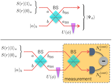
Figure 1: (Top) Scheme of the interferometer: the two input states $\left|{\psi}\right\rangle_{a}\otimes\left|{\alpha}\right\rangle_{b}$ interfere at a 50:50 beam splitter (BS) and one of the two transmitted beams undergoes a phase shift $\phi$. (Bottom) Scheme of the Mach-Zehnder interferometer: after the phase shift the two modes are mixed at a BS and the difference photocurrent is recorded.

In our analysis we address two possible couples of states $\left|{\psi}\right\rangle_{a}\otimes\left|{\alpha}\right\rangle_{b}$ for the two input modes $a$ and $b$ (with $[b,b^{{\dagger}}]=[a,a^{{\dagger}}]=\mathbbm{I}$, $\left[a,b\right]=0$), where the mode $b$ is excited in a coherent state, whereas $\left|{\psi}\right\rangle_{a}$ can be either the SqSPh $S(r)\left|{1}\right\rangle_{a}$ or the SqVac $S(r)\left|{0}\right\rangle_{a}$, where $S(r)=\exp\left[\frac{1}{2}r({a^{{\dagger}}}^{2}-a^{2})\right]$ is the squeezing operator, as depicted in the top panel of Fig. 1. The input modes interfere at a 50:50 beam splitter (BS), let $a_{\rm BS}=(a+b)/\sqrt{2}$ and $b_{\rm BS}=(b-a)/\sqrt{2}$ be the Heisenberg evolution of the initial mode operators $a$ and $b$, after the passage through BS. Then one of the modes, say $a_{\rm BS}$, undergoes a phase shift of amount $\phi$, described by the operator $U\left(\phi\right)=\exp\left(i\phi\,a_{\rm BS}^{\dagger}a_{\rm BS}\right)$, we want to estimate. To this aim we first choose a suitable measurement, usually described by a positive-operator-valued measurement $\{\Pi_{x}\}$, whose outcomes $x$ depend on the parameter $\phi$ and are distributed according to the conditional probability $p(x|\phi)=\left\langle{\Psi_{\phi}}\right|\Pi_{x}\left|{\Psi_{\phi}}\right\rangle$, $\left|{\Psi_{\phi}}\right\rangle$ being the two-mode state coming from the interferometer (see the top panel of Fig. 1). Starting from the data, we define an estimator, namely, a function function providing the value of the $\phi$ and its variance $\Delta^{2}\phi$.

In classical estimation theory the Cramér-Rao imposes a lower bound to variance (we drop for the sake of simplicity the statistical scaling):

$$\Delta^{2}\phi\geq\frac{1}{F\left(\phi\right)}$$

$F\left(\phi\right)$ being the Fisher information:

$$F\left(\phi\right)=\int_{\Lambda}p(x|\phi)\left[\partial_{\phi}\log p(x|\phi)\right]^{2},$$

where $\Lambda$ is the data sample space. However, the Cramér-Rao refers to the actual chosen measurement. Using the tools of quantum estimation theory par:QEQT , we can look for the optimal measurement minimising the uncertainty or, equivalently, maximising the Fisher information. Therefore, we can introduce the so-called quantum Fisher information hel76 ; bro9x :

$$Q_{\rm F}\left(\phi\right)=\mbox{Tr}\left[\rho_{\phi}\,L_{\phi}^{2}\right],$$

where $\rho_{\phi}=\left|{\Psi_{\phi}}\right\rangle\left\langle{\Psi_{\phi}}\right|$ and $L_{\phi}$ is the symmetric logarithmic derivative, $\partial_{\phi}\rho_{\phi}=(L_{\phi}\rho_{\phi}+\rho_{\phi}L_{\phi})/2$. By definition, $Q_{\rm F}\left(\phi\right)\geq F\left(\phi\right)$, thus we obtain the quantum Cramér-Rao bound bra94 ; bra96 :

$$\Delta^{2}\phi\geq\frac{1}{Q_{\rm F}\left(\phi\right)}.$$

Since we are addressing a family of pure states which come to depend on the parameter $\phi$ through a unitary operator of the form $U_{\phi}=\exp(-i\phi G)$, where $G=a^{\dagger}_{\rm BS}a_{\rm BS}$ is the Hermitian generator, the quantum Fisher information can be evaluated as par:QEQT :

$$Q_{\rm F}=4\left\langle\Psi_{\rm in}\right|\Delta^{2}G\left|\Psi_{\rm in}\right\rangle,$$ (1)

$\left|\Psi_{\rm in}\right\rangle=\left|\psi\right\rangle_{a}\otimes\left|\alpha\right\rangle_{b}$ being the quantum state entering the interferometer (see the top panel of Fig. 1), which is thus independent of $\phi$.

Up to now we have considered the optimal scenario based on the optimal measurement. However, in practice one should choose a particular detection scheme, according to the current technology. In the bottom panel of Fig. 1 we depict a typical Mach-Zehnder interferometer, where during the measurement stage the two modes interfere at a second BS before a photodetection process, which measures the difference photocurrent between the two output modes $a_{\rm out}$ and $b_{\rm out}$, namely:

$$O(\phi)=\left\langle{\Psi_{\rm in}}\right|N_{a}^{\rm(out)}-N_{b}^{\rm(out)}\left|{\Psi_{\rm in}}\right\rangle,$$ (2)

with $N_{k}^{\rm(out)}=k^{{\dagger}}_{\rm out}k_{\rm out}$, $k=a,b$. It is worth noting that given a small fluctuation $\delta\phi$, we can write:

$$O(\phi+\delta\phi)\approx O(\phi)+\partial_{\phi}O(\phi)\,\delta\phi,$$

and, thus, we have the following change of the photocurrent difference:

$$O(\phi+\delta\phi)-O(\phi)\approx\partial_{\phi}O(\phi)\,\delta\phi.$$

In order to detect such a difference we should require that $\left[O(\phi+\delta\phi)-O(\phi)\right]^{2}\gtrsim\Delta^{2}O(\phi)$ or, equivalently, $|\partial_{\phi}O(\phi)\,\delta\phi|\gtrsim\sqrt{\Delta^{2}O(\phi)}$. Therefore, there is a minimum value that can be detected by the apparatus, which is the sensitivity of the interferometer given by:

$$s\left(\phi\right)=\frac{\sqrt{\Delta^{2}O(\phi)}}{\left|\partial_{\phi}O(\phi)\right|}.$$ (3)

It is possible to show CS:16 that the sensitivity is lower bounded by the inverse of the Fisher information associated with the measurement, and we have:

$$s\left(\phi\right)\gtrsim\frac{1}{\sqrt{F\left(\phi\right)}}\geqslant\frac{1}{\sqrt{Q_{\rm F}}}.$$ (4)

In the following we will evaluate the quantum Fisher information and the Fisher information considering as input states a SqSPh or a SqVac and a CS and we will compare the performance of the interferometer.

III Quantum Fisher information

In order to have the same squeezing factor and total number of photons $N_{\rm tot}\geq 1$, we rewrite the two two-mode input states as follows (without loss of generality we can assume the squeezing parameter $r$ and the CS amplitude $\gamma$ to be real):

$$\left|{\Psi_{\rm in}^{\rm(SqSPh)}}\right\rangle =S(r)\left|{1}\right\rangle_{a}\otimes\left|{\sqrt{N_{\rm tot}-(\cosh 2r+\sinh^{2}r)}}\right\rangle_{b},$$ (5a)

$$\left|{\Psi_{\rm in}^{\rm(SqVac)}}\right\rangle =S(r)\left|{0}\right\rangle_{a}\otimes\left|{\sqrt{N_{\rm tot}-\sinh^{2}r}}\right\rangle_{b},$$ (5b)

or:

$$\left|{\Psi_{\rm in}^{\rm(SqSPh)}}\right\rangle =S(r)\left|{1}\right\rangle_{a}\otimes\left|{\gamma}\right\rangle_{b},$$ (6a)

$$\left|{\Psi_{\rm in}^{\rm(SqVac)}}\right\rangle =S(r)\left|{0}\right\rangle_{a}\otimes\left|{\sqrt{\gamma^{2}+\cosh 2r}}\right\rangle_{b},$$ (6b)

where we introduced the (real) coherent amplitude $\gamma$, so that $N_{\rm tot}=\gamma^{2}+\cosh 2r+\sinh^{2}r$. The second parametrisation can be more useful since, in a typical setup, one fixes the squeezing parameter $r$ and the CS amplitude $\gamma$ (note that in order to have the same $N_{\rm tot}$ the CS which interferes with the SqVac should have a larger energy than the one interfering with the SqSPh).

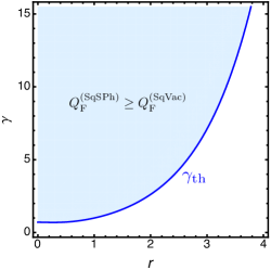
Figure 2: Plot of the threshold $\gamma_{\rm th}(r)$: for $\gamma>\gamma_{\rm th}(r)$ we have $Q_{\rm F}^{\rm(SqSPh)}(\gamma,r)\geq Q_{\rm F}^{\rm(SqVac)}(\gamma,r)$ (shaded region). See the text for details.

Exploiting Eq. (1) and Eqs. (6), we can compare the quantum Fisher information in the two cases, namely $Q_{\rm F}^{\rm(SqSPh)}(\gamma,r)$ and $Q_{\rm F}^{\rm(SqVac)}(\gamma,r)$. Though the calculation is quite straightforward, the analytical results are cumbersome and they are not explicitly reported here; we just observe that the quantum Fisher information is maximised for $\phi=\pi/2$ and this will be our working point throughout the rest of the paper.

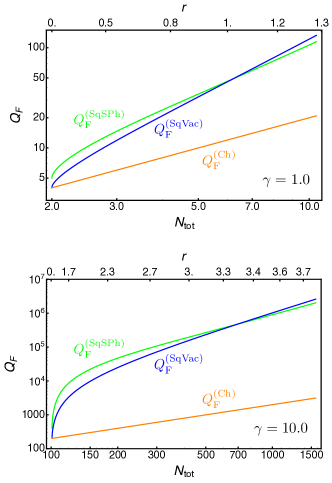
Figure 3: Plots of the of $Q_{\rm F}^{\rm(SqSPh)}$ and $Q_{\rm F}^{\rm(SqVac)}$ as functions of $N_{\rm tot}$ (lower horizontal axis) or $r$ (upper horizontal axis) for two values of the coherent amplitude: $\gamma=1.0$ (top panel) and $\gamma=10.0$ (bottom panel). Note that increasing $N_{\rm tot}$ corresponds to add squeezing to the system. As expected from Fig. 2, we can identify a low energy regime where $Q_{\rm F}^{\rm(SqSPh)}\geq Q_{\rm F}^{\rm(SqVac)}$. As $N_{\rm tot}$ gets larger the Heisenberg scaling $\propto N_{\rm tot}^{2}$ is reached. For comparison, we also show the quantum Fisher information $Q_{\rm F}^{\rm(Ch)}=2N_{\rm tot}$ (orange lines) referring to a single coherent state mixed with the vacuum (in this case the upper axis is meaningless). See the text for details.

In Fig. 2 we plot the region of the $r\gamma$–plane for which $Q_{\rm F}^{\rm(SqSPh)}(\gamma,r)\geq Q_{\rm F}^{\rm(SqVac)}(\gamma,r)$: given the squeezing parameter $r$ there is a threshold value

$$\gamma_{\rm th}(r)=\frac{1}{2}{\rm e}^{-r}\sqrt{2+\sinh 4r},$$

such that for $\gamma>\gamma_{\rm th}(r)$ the SqSPh outperforms SqVac. It is worth noting that for each point in Fig. 2 the quantum Fisher information $Q_{\rm F}^{\rm(SqSPh)}(\gamma,r)$ and $Q_{\rm F}^{\rm(SqVac)}(\gamma,r)$ refer to states with the same $N_{\rm tot}$ according to the parametrisation in Eqs. (6). In Fig. 3 we plot the two quantum Fisher information as functions of $N_{\rm tot}$ (or $r$) and fixed value of the coherent amplitude $\gamma$. In this cases we have the following asymptotic behaviour in the high number of photons limit $N_{\rm tot}\gg 1$ (or large squeezing parameter $r$):

$$Q_{\rm F}^{\rm(SqSPh)} \approx\frac{2}{3}N_{\rm tot}^{2},$$ (7)

$$Q_{\rm F}^{\rm(SqVac)} \approx\frac{10}{9}N_{\rm tot}^{2},$$ (8)

respectively, that is in both the cases we find the Heisenberg scaling as one may expect pez08 ; CS:JOSAB . It is worth noting that, at least in the presence of the optimal measurement, the squeezing resource allows outperforming the coherent light. This is clear form Fig. 3, where we also show the behaviour of the quantum Fisher information $Q_{\rm F}^{\rm(SqSPh)}=2N_{\rm tot}$ for a coherent state mixed with the vacuum.

IV Sensitivity

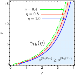
Figure 4: Plot of the threshold $\tilde{\gamma}_{\rm th}(\eta)$: for $\gamma\leq\tilde{\gamma}_{\rm th}(\eta)$ we have $s^{\rm(SqVac)}(\gamma,r;\eta)\geq s^{\rm(SqSPh)}(\gamma,r;\eta)$ (shaded regions). The colors refers to different values of the quantum efficiency. Note that the lower is the quantum efficiency, the larger is the region in which SqSPh performs better than SqVac. See the text for details.

In this section we address the sensitivity of the Mach-Zehnder interferometer setup sketched in the bottom panel of Fig. 1. As in the case concerning the quantum Fisher information, also the calculation of the sensitivity, as defined in Eq. (3), can be straightforwardly obtained starting from the input states (6). The analytical results are clumsy and they are not reported explicitly.

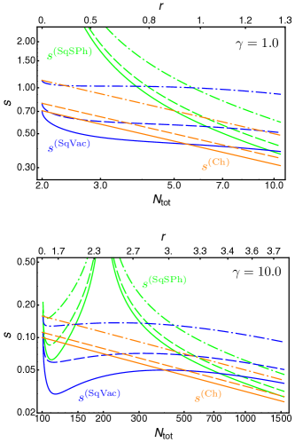
Figure 5: Plots of the sensitivity $s^{\rm(SqSPh)}$ (green lines) and $s^{\rm(SqVac)}$ (blue lines) as functions of $N_{\rm tot}$ (lower horizontal axis) or $r$ (upper horizontal axis) for two values of the coherent amplitude ($\gamma=1.0$ (top panel) and $\gamma=10.0$ (bottom panel)) and different values of the quantum efficiency: $\eta=1.0$ (solid lines), $\eta=0.8$ (dashed lines) and $\eta=0.4$ (dot-dashed lines). Note that increasing $N_{\rm tot}$ corresponds to add squeezing to the system. As expected from Fig. 4, we can identify a high energy regime where $s^{\rm(SqSPh)}\leq s^{\rm(SqVac)}$ (SqSPh performs better). As $N_{\rm tot}$ gets larger the shot-noise scaling $\propto N_{\rm tot}^{-1/2}$ is reached. For comparison, we also plotted the sensitivity $s^{\rm(Ch)}=(\eta N_{\rm tot})^{-1/2}$ (orange lines) referring to a coherent state mixed with the vacuum (in this case the upper axis is meaningless). See the text for details.

In Fig. 4 we plot the sensitivities $s^{\rm(SqSPh)}(\gamma,r;\eta)$ and $s^{\rm(SqVac)}(\gamma,r;\eta)$, where $\eta$ is the quantum efficiency of the photodetectors FOP:05 ; the comparison is obtained for fixed total number of photons $N_{\rm tot}$ (we recall that $\gamma$ is the amplitude of the CS interfering with the SqSPh, therefore, in general, the two configurations have the same total energy, same squeezing parameter $r$ but different coherent amplitude). With respect to the quantum Fisher information (see Fig. 2), we can see that for fixed $r$ now we have a threshold $\tilde{\gamma}_{\rm th}$ of the coherent amplitude below which SqSPh outperforms SqVac. Moreover, as the quantum efficiency becomes lower, the actual value of $\tilde{\gamma}_{\rm th}$ increases: losses at the detection are more detrimental for a setup based on SqVac.

In Fig. 5 we plot $s^{\rm(SqSPh)}$ and $s^{\rm(SqVac)}$ for two fixed values of $\gamma$. In the same plots we also report $s^{\rm(Ch)}=(\eta N_{\rm tot})^{-1/2}$, that is the sensitivity obtained when a coherent state with amplitude $\sqrt{N_{\rm tot}}$ and the vacuum state are considered as inputs. In this case we find the following scaling for the high photon number regime $N_{\rm tot}\gg 1$ (or large squeezing parameter $r$):

$$s^{\rm(SqSPh)} \approx\frac{1}{\sqrt{\eta\,N_{\rm tot}}}\,\equiv s^{\rm(Ch)},$$ (9)

$$s^{\rm(SqVac)} \approx\sqrt{\frac{3(3-2\eta)}{\eta\,N_{\rm tot}}},$$ (10)

respectively, that is in both the case we find the shot-noise limit $\propto N_{\rm tot}^{-1/2}$: in this limit the SqSPh performs better that SqVac.

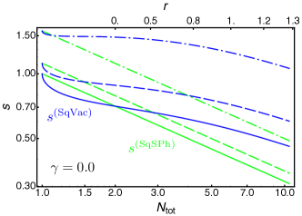
Figure 6: Plots of the sensitivity $s^{\rm(SqSPh)}$ (green lines) and $s^{\rm(SqVac)}$ (blue lines) as functions of $N_{\rm tot}$ (lower horizontal axis) or $r$ (upper horizontal axis) for $\gamma=0.0$ and different values of the quantum efficiency: $\eta=1.0$ (solid lines), $\eta=0.8$ (dashed lines) and $\eta=0.4$ (dot-dashed lines). Note that we have $s^{\rm(SqSPh)}=s^{\rm(Ch)}=(\eta N_{\rm tot})^{-1/2}$.

Inspecting Fig. 4, it is interesting to note when the SqSPh is mixed with the vacuum ($\gamma=0$), there is a minimum value of the squeezing parameter $r$ above which a SqSPh allows reaching a better sensitivity than a setup exploiting SqVac mixed with a suitable CS in order to have the same $N_{\rm tot}$ (see also Fig. 6). However, in this last case one have $s^{\rm(SqSPh)}=s^{\rm(Ch)}=(\eta N_{\rm tot})^{-1/2}$, namely, the squeezed single photon performs as a coherent state with the same energy.

V Conclusions

In this manuscript we have investigated the performance of a SqSPh as a probe to detect some optical phase shift. We have carried out our analysis comparing the results from the interference of the SqSPh with a CS and with the results obtained addressing a SqVac. In particular we focused on the case of fixed squeezing parameter (assumed to be the same for the SqSPh and the SqVac) and fixed total number of photons. Addressing both the quantum Fisher information and the Mach-Zehnder interferometer (based on photodetectors), we have found the regimes in which a SqSPh can outperform a SqVac as input. Our results show that whereas in the optimal case, i.e., the case involving the optimal measurement associated with the quantum Fisher information, both the inputs allow reaching the Heisenberg scaling in the high energy (or squeezing) limit (though SqVac performs better), when the measurement of the different photocurrent is considered the interferometer exploiting a SqSPh exhibits a better sensitivity. Eventually, we also presented some results (see the top panel plots of Figs. 5 and 6) based on parameters that can be experimentally reachable considering the small amount of the total energy (up ten photons) and the reasonable amount of squeezing (below $12$ dB corresponding to $r\approx 1.38$.) DD:13 .

References

- (1) M. Kacprowicz, R. Demkowicz-Dobrzanski, W. Wasilewski, K. Banaszek, and I. A. Walmsley, “Experimental quantum-enhanced estimation of a lossy phase shift”, Nature Phot. 4, 357 (2010).
- (2) J. Abadie, et al. (the LIGO Scientific Collaboration), A gravitational wave observatory operating beyond the quantum shot-noise limit, Nat. Phys. 7, 962 (2011).
- (3) R. Demkowicz-Dobrzański, K. Banaszek, and R. Schnabel, “Fundamental quantum interferometry bound for the squeezed- light-enhanced gravitational wave detector GEO 600”, Phys. Rev. A 88, 041802(R) (2013).
- (4) I. Ruo Berchera, I. P. Degiovanni, S. Olivares, and M. Genovese, “Quantum light in coupled interferometers for quantum gravity tests”, Phys. Rev. Lett. 110, 213601 (2013).
- (5) I. Ruo-Berchera, I. P. Degiovanni, S. Olivares, N. Samantaray, P. Traina, and M. Genovese, “One- and two-mode squeezed light in correlated interferometry”, Phys. Rev. A 92, 053821 (2015).
- (6) M. G. A. Paris, “Small amount of squeezing in high-sensitive realistic interferometry”, Phys. Lett A 201, 132 (1995)
- (7) L. Pezzé, and A. Smerzi, “Mach-Zehnder Interferometry at the Heisenberg Limit with Coherent and Squeezed-Vacuum Light”, Phys. Rev. Lett. 100, 073601 (2008).
- (8) S. Olivares, and M. G. A. Paris, “Optimized Interferometry with Gaussian States”, Optics Spectr. 103, 231 (2007).
- (9) M. D. Lang, and C. M. Caves, “Optimal Quantum-Enhanced Interferometry Using a Laser Power Source”, Phys. Rev. Lett. 111, 173601 (2013).
- (10) M. D. Lang, and C. M. Caves, “Optimal quantum-enhanced interferometry”, Phys. Rev. A 90, 025802 (2014).
- (11) C. Sparaciari, S. Olivares, and M. G. A. Paris, “Bounds to precision for quantum interferometry with Gaussian states and operations”, J. Opt. Soc. Am. B 32, 1354 (2015).
- (12) R. Demkowicz-Dobrzański, M. Jarzyna, and J. Kołodyński, “Quantum Limits in Optical Interferometry”, Progress in Optics 60, 345 (2015).
- (13) C. Sparaciari, S. Olivares, and M. G. A. Paris, “Gaussian-state interferometry with passive and active elements”, Phys. Rev. A 93, 023810 (2016).
- (14) P. Sekatski, N. Sangouard, M. Stobińska, F. Bussières, M. Afzelius, and N. Gisin, “Proposal for exploring macroscopic entanglement with a single photon and coherent states”, Phys. Rev. A 86, 060301(R) (2012).
- (15) C. Vitelli, N. Spagnolo, L. Toffoli, F. Sciarrino, and F. De Martini, “Enhanced resolution of lossy interferometry by coherent amplification of single photons”, Phys. Rev. Lett. 105, 113602 (2010)
- (16) J. Wenger, R. Tualle-Bouri, and P. Grangier, “Non-Gaussian Statistics from Individual Pulses of Squeezed Light”, Phys. Rev. Lett. 92 153601 (2004).
- (17) S. Olivares, and M. G. A. Paris, “Squeezed Fock state by inconclusive photon subtraction”, J. Opt. B: Quantum Semiclass. Opt. 7, S616 (2005).
- (18) M. G. A. Paris, “Quantum estimation for quantum technology”, Int. J. Quant. Inf. 7, 125 (2009).
- (19) C. W. Helstrom, Quantum Detection and Estimation Theory (Academic Press, New York, 1976).
- (20) D. C. Brody, and L. P. Hughston, “Statistical geometry in quantum mechanics”, Proc. Roy. Soc. Lond. A 454, 2445 (1998); “Geometrization of statistical mechanics”, Proc. Roy. Soc. Lond. A 455, 1683 (1999).
- (21) S. L. Braunstein, and C. M. Caves, “Statistical distance and the geometry of quantum states”, Phys. Rev. Lett. 72, 3439 (1994).
- (22) S. L. Braunstein, C. M. Caves, and G. J. Milburn, “Generalized uncertainty relations: Theory, examples, and Lorentz invariance”, Ann. Phys. 247, 135 (1996).
- (23) A. Ferraro, S. Olivares, and M. G. A. Paris, Gaussian States in Quantum Information (Bibliopolis, Napoli, 2005).