Exponential collocation methods for
the cubic Schrödinger equation

Abstract

In this paper we derive and analyse new exponential collocation methods to efficiently solve the cubic Schrödinger Cauchy problem on a $d$-dimensional torus. Energy preservation is a key feature of the cubic Schrödinger equation. It is proved that the novel methods can be of arbitrarily high order which exactly or nearly preserve the continuous energy of the original continuous system. The existence and uniqueness, regularity, global convergence, nonlinear stability of the new methods are studied in detail. Two practical exponential collocation methods are constructed and two numerical experiments are included. The numerical results illustrate the efficiency of the new methods in comparison with existing numerical methods in the literature.

Keywords: Cubic Schrödinge equation, Energy preservation,Exponential integrators, Collocation methods

MSC: 65P1035Q5565M1265M70

1 Introduction

It is well known that one of the cornerstones of quantum physics is the Schrödinger equation. The nonlinear Schrödinger equation has long been used to approximately describe the dynamics of complicated systems, such as Maxwell s equations for the description of nonlinear optics or the equations describing surface water waves, including rogue waves which appear from nowhere and disappears without a trace (see, e.g. [1, 2, 3]). This paper is devoted to designing and analysing novel numerical integrators to efficiently solve the cubic Schrödinger equation

$$\left\{\begin{aligned} &\mathrm{i}u_{t}+\triangle u=\lambda|u|^{2}u,\ \ (t,x)\in[0,T]\times\mathbb{T}^{d},\\ &u(0,x)=u_{0}(x),\ \ \ \ \ \ x\in\mathbb{T}^{d},\end{aligned}\right.$$ (1)

where $\mathbb{T}$ is denoted the one-dimensional torus $\mathbb{R}/(2\pi\mathbb{Z})$ and for the given positive integer $d$, $\mathbb{T}^{d}$ denotes the $d$-dimensional torus. It is noted that following the researches in [4, 5, 6], we only consider the cubic Schrödinger equation in this paper. With the techniques developed and used in this paper, it is also feasible to extend the novel approach to general Schrödinger equations. In this paper, we consider this equation as a Cauchy problem in time (no space discretisation is made). The solutions of this equation have conservation of the following energy

$$H[u]=\frac{1}{2(2\pi)^{d}}\int_{\mathbf{T}^{d}}\Big{(}|\nabla u|^{2}+\frac{\lambda}{2}|u|^{4}\Big{)}dx.$$ (2)

It is of great interest to devise numerical schemes which can conserve the continuous version of this important invariant, and the aim of this paper is to formulate a novel kind of exponential integrators with a good property of continuous energy preservation.

Schrödinger equations frequently arise in a wide variety of applications including several areas of physics, fiber optics, quantum transport and other applied sciences (see, e.g. [7, 8, 9, 10, 11]). Many numerical methods have been proposed for the integration of Schrödinger equations, such as splitting methods (see, e.g. [6, 12, 13, 14, 15, 16, 17]), exponential-type integrators (see, e.g. [4, 18, 19, 20, 21]), multi-symplectic methods (see, e.g. [22, 23]) and other effective methods (see, e.g. [24, 25, 26, 27]).

In recent decades, structure-preserving algorithms of differential equations have been received much attention and for the related work, we refer the reader to [28, 29, 30, 31, 32, 33, 34, 35] and references therein. It is well known that structure-preserving algorithms are able to exactly preserve some structural properties of the underlying continuous system. Amongst the typical subjects of structure-preserving algorithms are energy-preserving schemes, which exactly preserve the energy of the underlying system. There have been a lot of studies on this topic for Hamiltonian partial differential equations (PDEs). In [36], finite element methods were introduced systematically for numerical solution of PDEs. The authors in [37, 38] researched discrete gradient methods for PDEs. The work in [39] investigated the average vector field (AVF) method for discretising Hamiltonian PDEs. Hamiltonian Boundary Value Methods (HBVMs) were studied for the semilinear wave equation in [40] and were recently researched for nonlinear Schrödinger equations with wave operator in [41]. The adapted AVF method for Hamiltonian wave equations was analysed in [42, 43]. Other related work is referred to [44, 45, 46, 47, 48, 49, 50, 51]. On the other hand, exponential integrators have been widely introduced and developed for solving first-order ODEs, and we refer the reader to [29, 52, 53, 54, 55] for example. This kind of methods has also been studied in the numerical integration of Schrödinger equations (see, e.g. [4, 18, 19, 20, 21]). However, it seems that until now, exponential integrators with a good continuous energy preservation for Schrödinger equations, have not been studied in the literature, which motivates this paper.

With this premise, this paper is mainly concerned with exponential collocation methods for solving cubic Schrödinger equations. The remainder of this paper is organized as follows. We first present some notations and preliminaries in Section 2. Then the scheme of exponential collocation methods is formulated and a good continuous energy preservation is proved in Section 3. In Section 4, we analyse the existence, uniqueness and smoothness of the methods. Section 5 pays attention to the regularity. The convergence of the methods is studied in Section 6 and the nonlinear stability is discussed in Section 7. Section 8 is devoted to constructing practical exponential collocation methods in the light of the approach proposed in this paper, and reporting two numerical experiments to demonstrate the excellent qualitative behavior of the new methods. Section 9 focuses on the concluding remarks.

2 Notations and preliminaries

In this paper, we use the following notations which were presented in [20].

• We denote by $L^{2}(\mathbb{T}^{d})$ (or simply $L^{2}$) the set of (classes of) complex functions $f$ on $\mathbb{T}^{d}$ such that $\int_{\mathbb{T}^{d}}|f(x)|^{2}dx<+\infty$, endowed with the norm $\left\|f\right\|_{L^{2}(\mathbb{T}^{d})}=\big{(}(2\pi)^{-d}\int_{\mathbb{T}^{d}}|f(x)|^{2}dx\big{)}^{1/2}.$

• For $\alpha\in\mathbb{R}^{+}$, denote by $H^{\alpha}(\mathbb{T}^{d})$ (or simply $H^{\alpha}$) the space of (classes of) complex functions $f\in L^{2}(\mathbb{T}^{d})$ such that $\sum_{k\in\mathbb{Z}^{d}\backslash\{0\}}|\hat{f}_{k}|^{2}|k|_{2}^{2\alpha}<+\infty,$ endowed with the norm $\left\|f\right\|_{H^{\alpha}}=\Big{(}|\hat{f}_{0}|^{2}+\sum_{k\in\mathbb{Z}^{d}\backslash\{0\}}|\hat{f}_{k}|^{2}|k|_{2}^{2\alpha}\Big{)}^{1/2},$ where $\hat{f}_{k}=(2\pi)^{-d}\int_{\mathbb{T}^{d}}f(x)e^{-\mathrm{i}kx}dx.$ Note that $L^{2}=H^{0}$ with the same norm.

• For the operators $A$ from $H^{\alpha}$ to itself, we denote $\|A\|_{H^{\alpha}\rightarrow H^{\alpha}}=\sup\limits_{v\in H^{\alpha},v\neq 0}\frac{\|Av\|_{H^{\alpha}}}{\|v\|_{H^{\alpha}}}.$

The following result given in [20] will be useful for the analysis of this paper.

Proposition 1

(See [20].) With the above notations, if $\varphi$ is a function from $\mathbb{C}$ to $\mathbb{C}$ bounded by $M\geq 0$ on $\textmd{i}\mathbb{R}$, then for all $h>0$ and $\alpha\geq 0$, we have

$$\left\|\varphi(\textmd{i}h\Delta)\right\|_{H^{\alpha}\rightarrow H^{\alpha}}\leq M.$$

For example, for all $\alpha\geq 0$, it is true that $\left\|e^{\textmd{i}h\Delta}\right\|_{H^{\alpha}\rightarrow H^{\alpha}}=1.$

In order to derive the novel methods, we will use the idea of continuous time finite element methods in a generalised function space. To this end, we first present the following three definitions.

Definition 1

Define the generalised function space on $[0,T]\times\mathbb{T}^{d}$ as follows:

$$Y(t,x)= \textmd{span}^{x}\left\{\varphi_{0}(t),\ldots,\varphi_{r-1}(t)\right\}=\{w:w(t,x)=\sum_{j=0}^{r-1}\varphi_{j}(t)U_{j}(x),~{}U_{j}(x):=\left(\begin{array}[]{c}U_{j}^{1}(x)\\ U_{j}^{2}(x)\\ \end{array}\right),$$

$$\ \ \ \ \quad U_{j}^{1}(x),U_{j}^{2}(x)\ \textmd{are arbitrary functions in}\ H^{\alpha}(\mathbb{T}^{d})\},$$

where $r$ is an integer satisfying $r\geq 1$ and the functions $\{\varphi_{j}(t)\}_{j=0}^{r-1}:[0,T]\rightarrow\mathbb{C}$ are supposed to be linearly independent, sufficiently smooth and integrable.

In this paper, we consider two generalised function spaces $X(t,x)$ and $Y(t,x)$ such that $w_{t}(t,x)\in Y(t,x)$ for any $w(t,x)\in X(t,x)$. Then choose a time stepsize $h$ and define $Y_{h}(\tau,x)$ and $X_{h}(\tau,x)$ as

$$Y_{h}(\tau,x)=Y(\tau h,x),\ X_{h}(\tau,x)=X(\tau h,x),$$ (3)

where $\tau$ is a variable satisfying $\tau\in[0,1]$. It is noted that throughout this paper, the notations $\tilde{\varphi}(\tau)$ and $\tilde{f}(\tau,x)$ are referred to as $\varphi(\tau h)$ and $f(\tau h,x)$ for all the functions, respectively.

Definition 2

The inner product for the time is defined by

$$\langle\tilde{w}_{1}(\tau,x),\tilde{w}_{2}(\tau,x)\rangle_{\tau}=\int_{0}^{1}\tilde{w}_{1}(\tau,x)\cdot\tilde{w}_{2}(\tau,x)d\tau,$$

where $\tilde{w}_{1}(\tau,x)$ and $\tilde{w}_{2}(\tau,x)$ are two integrable functions for $\tau$ (scalar-valued or vector-valued) on $[0,1]$, and if they are both vector-valued functions, ‘$\cdot$’ denotes the entrywise multiplication operation.

Definition 3

A projection $\mathcal{P}_{h}\tilde{w}(\tau,x)$ onto $Y_{h}(\tau,x)$ is defined as

$$\langle\tilde{v}(\tau,x),\mathcal{P}_{h}\tilde{w}(\tau,x)\rangle_{\tau}=\langle\tilde{v}(\tau,x),\tilde{w}(\tau,x)\rangle_{\tau},\quad\text{for any}\ \ \tilde{v}(\tau,x)\in Y_{h}(\tau,x),$$ (4)

where $\tilde{w}(\tau,x)$ is a continuous two-dimensional vector function for $\tau\in[0,1]$.

With regard to the projection operation $\mathcal{P}_{h}$, the following property is important.

Lemma 1

The projection $\mathcal{P}_{h}\tilde{w}$ can be explicitly expressed as

$$\mathcal{P}_{h}\tilde{w}(\tau,x)=\langle P_{\tau,\sigma},\tilde{w}(\sigma,x)\rangle_{\sigma},$$

where $P_{\tau,\sigma}=\sum_{j=0}^{r-1}\tilde{\psi}_{j}(\tau)\tilde{\psi}_{j}(\sigma),$ and $\{\tilde{\psi}_{j}(\tau)\}_{j=0,\ldots,r-1}$ is a standard orthonormal basis of $Y_{h}(\tau,x)$.

Proof Since $P_{h}\tilde{w}(\tau,x)\in Y_{h}(\tau,x)$, it can be expressed as $P_{h}\tilde{w}(\tau,x)=\sum_{k=0}^{r-1}\tilde{\psi}_{k}(\tau)U_{k}(x).$ By taking $\tilde{v}(\tau)=\tilde{\psi}_{l}(\tau)e_{j}\in Y_{h}(\tau,x)$ in (4) for $l=0,1,\ldots,r-1$ and $j=1,2$, we obtain

$$\langle\tilde{\psi}_{l}(\tau)e_{j},\sum_{k=0}^{r-1}\tilde{\psi}_{k}(\tau)U_{k}(x)\rangle_{\tau}=\sum_{k=0}^{r-1}\langle\tilde{\psi}_{l}(\tau)e_{j},\tilde{\psi}_{k}(\tau)U_{k}(x)\rangle_{\tau}$$

$$= \sum_{k=0}^{r-1}\langle\tilde{\psi}_{l}(\tau),\tilde{\psi}_{k}(\tau)\rangle_{\tau}(e_{j}\cdot U_{k}(x))=\langle\tilde{\psi}_{l}(\tau)e_{j},\tilde{w}(\tau,x)\rangle_{\tau},$$

which gives $\sum_{k=0}^{r-1}\langle\tilde{\psi}_{l}(\tau),\tilde{\psi}_{k}(\tau)\rangle_{\tau}U_{k}(x)=\langle\tilde{\psi}_{l}(\tau),\tilde{w}(\tau,x)\rangle_{\tau}.$ By the standard orthonormal basis $\{\tilde{\psi}_{j}(t)\}_{j=0,\ldots,r-1}$, this result can be formulated as

$$\left(\begin{array}[]{c}U_{0}(x)\\ \vdots\\ U_{r-1}(x)\end{array}\right)=\left(\begin{array}[]{c}\langle\tilde{\psi}_{0}(\tau),\tilde{w}(\tau,x)\rangle_{\tau}\\ \vdots\\ \langle\tilde{\psi}_{r-1}(\tau),\tilde{w}(\tau,x)\rangle_{\tau}\end{array}\right).$$

Then one has

$$P_{h}\tilde{w}(\tau,x)=(\tilde{\psi}_{0}(\tau),\ldots,\tilde{\psi}_{r-1}(\tau))\otimes I_{2\times 2}\left(\begin{array}[]{c}U_{0}(x)\\ \vdots\\ U_{r-1}(x)\end{array}\right)$$

$$= (\tilde{\psi}_{0}(\tau),\ldots,\tilde{\psi}_{r-1}(\tau))\otimes I_{2\times 2}\left(\begin{array}[]{c}\langle\tilde{\psi}_{0}(\tau),\tilde{w}(\tau,x)\rangle_{\tau}\\ \vdots\\ \langle\tilde{\psi}_{r-1}(\tau),\tilde{w}(\tau,x)\rangle_{\tau}\end{array}\right)=\langle P_{\tau,\sigma},\tilde{w}(\sigma,x)\rangle_{\sigma},$$

which proves the result. $\square$

Remark 1

It is noted that the above three definitions and Lemma 1 can be considered as the generalised version of those presented in [30]. We also remark that one can make different choices of $Y_{h}(\tau,x)$ and $X_{h}(\tau,x)$, which will produce different methods by taking the methodology proposed in this paper.

3 Formulation of exponential collocation methods

Define the linear differential operator $\mathcal{A}$ by

$$(\mathcal{A}u)(x,t)=\Delta u(x,t)$$

and let $f(u)=-\lambda|u|^{2}u$. Then the system (1) is identical to

$$u_{t}=\mathrm{i}\mathcal{A}u+\mathrm{i}f(u),\ \ \ \ u(0,x)=u_{0}(x).$$ (5)

The solutions of this equation satisfy Duhamel’s formula

$$u(t_{n}+h)=e^{\mathrm{i}h\mathcal{A}}u(t_{n})+\mathrm{i}\int_{0}^{h}e^{\mathrm{i}(h-\xi)\mathcal{A}}f(u(t_{n}+\xi))d\xi.$$ (6)

Let $u=p+\textmd{i}q,$ and then the equation (1) can be rewritten as a pair of real initial-value problems

$$\left(\begin{array}[]{c}p_{t}\\ q_{t}\\ \end{array}\right)=\begin{aligned} \left(\begin{array}[]{cc}0&-\mathcal{A}\\ \mathcal{A}&0\\ \end{array}\right)\left(\begin{array}[]{c}p\\ q\\ \end{array}\right)+\left(\begin{array}[]{c}\lambda(p^{2}+q^{2})q\\ -\lambda(p^{2}+q^{2})p\\ \end{array}\right)\end{aligned},\ \ \left(\begin{array}[]{c}p(0,x)\\ q(0,x)\\ \end{array}\right)=\left(\begin{array}[]{c}\textmd{Re}(u_{0}(x))\\ \textmd{Im}(u_{0}(x))\\ \end{array}\right).$$ (7)

In this case, the energy of this system is expressed by

$$\mathcal{H}(p,q)=\frac{1}{2(2\pi)^{d}}\int_{\mathbf{T}^{d}}\Big{(}|\nabla p|^{2}+|\nabla q|^{2}+\frac{\lambda}{2}(p^{2}+q^{2})^{2}\Big{)}dx.$$ (8)

Accordingly, the system (7) can be formulated as the following infinite-dimensional real Hamiltonian system

$$y_{t}=\mathcal{K}y+g(y)=J^{-1}\frac{\delta\mathcal{H}}{\delta y},\ \ \ \ y_{0}(x)=\left(\begin{array}[]{c}p(0,x)\\ q(0,x)\\ \end{array}\right),$$ (9)

where $\mathcal{K}=\left(\begin{array}[]{cc}0&-\mathcal{A}\\ \mathcal{A}&0\\ \end{array}\right),$ $J=\left(\begin{array}[]{cc}0&-1\\ 1&0\\ \end{array}\right),\ \ y=\left(\begin{array}[]{c}p\\ q\\ \end{array}\right),$ and $g(y)=\left(\begin{array}[]{c}\lambda(p^{2}+q^{2})q\\ -\lambda(p^{2}+q^{2})p\\ \end{array}\right).$

With the preliminaries described above, we first derive the exponential collocation methods for solving the real-valued equation (9) and then present the methods for solving the cubic Schrödinger equation (1).

We consider a function $\tilde{z}(\tau,x)$ with $\tilde{z}(0,x)=y_{0}(x)$, satisfying that

$$\tilde{z}_{t}(\tau,x) =\mathcal{K}\tilde{z}(\tau,x)+\mathcal{P}_{h}g(\tilde{z}(\tau,x))=\mathcal{K}\tilde{z}(\tau,x)+\langle P_{\tau,\sigma},g(\tilde{z}(\sigma,x))\rangle_{\sigma}.$$ (10)

Applying Duhamel’s formula (6) to (10) leads to

$$\tilde{z}(\tau,x)=e^{\tau h\mathcal{K}}y_{0}(x)+\tau h\int_{0}^{1}e^{(1-\xi)\tau h\mathcal{K}}\langle P_{\xi\tau,\sigma},g(\tilde{z}(\sigma,x))\rangle_{\sigma}d\xi$$

$$=e^{\tau h\mathcal{K}}y_{0}(x)+\tau h\int_{0}^{1}e^{(1-\xi)\tau h\mathcal{K}}\int_{0}^{1}\sum_{j=0}^{r-1}\tilde{\psi}_{j}(\xi\tau)\tilde{\psi}_{j}(\sigma)g(\tilde{z}(\sigma,x))d\sigma d\xi$$

$$=e^{\tau h\mathcal{K}}y_{0}(x)+\tau h\int_{0}^{1}\sum_{j=0}^{r-1}\int_{0}^{1}e^{(1-\xi)\tau h\mathcal{K}}\tilde{\psi}_{j}(\xi\tau)d\xi\tilde{\psi}_{j}(\sigma)g(\tilde{z}(\sigma,x))d\sigma.$$

This yields the following definition of exponential collocation methods.

Definition 4

An exponential collocation method for solving the real Hamiltonian initial-value problem (9) is defined by

$$\left\{\begin{aligned} &\tilde{z}(\tau,x)=e^{\tau h\mathcal{K}}y_{0}(x)+\tau h\int_{0}^{1}\bar{A}_{\tau,\sigma}(\mathcal{K})g(\tilde{z}(\sigma,x))d\sigma,\quad 0\leq\tau\leq 1,\\ &y_{1}(x)=\tilde{z}(1,x),\end{aligned}\right.$$ (11)

where $h$ is a time stepsize and

$$\bar{A}_{\tau,\sigma}(\mathcal{K})=\int_{0}^{1}e^{(1-\xi)\tau h\mathcal{K}}P_{\xi\tau,\sigma}d\xi=\sum_{i=0}^{r-1}\int_{0}^{1}e^{(1-\xi)\tau h\mathcal{K}}\tilde{\psi}_{i}(\xi\tau)d\xi\tilde{\psi}_{i}(\sigma).$$ (12)

Theorem 1

If $\tilde{z}(\tau,x)\in X_{h}(\tau,x)$, the continuous energy $\mathcal{H}$ determined by (8) is preserved exactly by the method (11), i.e.,

$$\mathcal{H}(y_{1}(x))=\mathcal{H}(y_{0}(x)).$$

If $\tilde{z}(\tau,x)\notin X_{h}(\tau,x)$, the exponential collocation method (11) approximately preserves the continuous energy $\mathcal{H}$ with the following accuracy

$$\mathcal{H}(y_{1}(x))=\mathcal{H}(y_{0}(x))+\mathcal{O}(h^{2r+1}).$$

Proof We first prove the first statement. Since $\tilde{z}(\tau,x)\in X_{h}(\tau,x)$, we obtain that $\tilde{z}_{t}(\tau,x)\in Y_{h}(\tau,x)$. Therefore, it follows from (10) that

$$\int_{0}^{1}\tilde{z}_{t}(\tau,x)^{\intercal}J^{\intercal}\tilde{z}_{t}(\tau,x)d\tau=\int_{0}^{1}\tilde{z}_{t}(\tau,x)^{\intercal}J^{\intercal}\big{(}\mathcal{K}\tilde{z}(\tau,x)+\mathcal{P}_{h}g(\tilde{z}(\tau,x))\big{)}d\tau$$ (13)

$$= \int_{0}^{1}\tilde{z}_{t}(\tau,x)^{\intercal}J^{\intercal}\big{(}\mathcal{K}\tilde{z}(\tau,x)+g(\tilde{z}(\tau,x))\big{)}d\tau.$$

Because $J$ is skew symmetric, we have

$$0=\int_{0}^{1}\tilde{z}_{t}(\tau,x)^{\intercal}J^{\intercal}\tilde{z}_{t}(\tau,x)d\tau=\int_{0}^{1}\tilde{z}_{t}(\tau,x)^{\intercal}J\big{(}\mathcal{K}\tilde{z}(\tau,x)+g(\tilde{z}(\tau,x))\big{)}d\tau.$$

Therefore, it is true that

$$\mathcal{H}(y_{1}(x))-\mathcal{H}(y_{0}(x))=\int_{0}^{1}\frac{\partial}{\partial\tau}\mathcal{H}(\tilde{z}(\tau,x))d\tau=h\int_{0}^{1}\tilde{z}_{t}(\tau,x)^{\intercal}\frac{\delta\mathcal{H}(\tilde{z})}{\delta\tilde{z}}d\tau$$

$$=h\int_{0}^{1}\tilde{z}_{t}(\tau,x)^{\intercal}J\big{(}\mathcal{K}\tilde{z}(\tau,x)+g(\tilde{z}(\tau,x))\big{)}d\tau=h\cdot 0=0.$$

For the second statement, according to the above analysis, we obtain

$$\mathcal{H}(y_{1}(x))-\mathcal{H}(y_{0}(x))=h\int_{0}^{1}\tilde{z}_{t}(\tau,x)^{\intercal}J\big{(}\mathcal{K}\tilde{z}(\tau,x)+g(\tilde{z}(\tau,x))\big{)}d\tau$$

$$= h\int_{0}^{1}\tilde{z}_{t}(\tau,x)^{\intercal}J\big{(}\mathcal{K}\tilde{z}(\tau,x)+\mathcal{P}_{h}g(\tilde{z}(\tau,x))+g(\tilde{z}(\tau,x))-\mathcal{P}_{h}g(\tilde{z}(\tau,x))\big{)}d\tau$$

$$= h\int_{0}^{1}\tilde{z}_{t}(\tau,x)^{\intercal}J\tilde{z}_{t}(\tau,x)+h\int_{0}^{1}\tilde{z}_{t}(\tau,x)^{\intercal}J\big{(}g(\tilde{z}(\tau,x))-\mathcal{P}_{h}g(\tilde{z}(\tau,x))\big{)}d\tau$$

$$= h\int_{0}^{1}\tilde{z}_{t}(\tau,x)^{\intercal}J\big{(}g(\tilde{z}(\tau,x))-\mathcal{P}_{h}g(\tilde{z}(\tau,x))\big{)}d\tau.$$

From the results of Lemmas 2-3 which are proved in Section 5, it follows that $\tilde{z}_{t}(\tau,x)=\mathcal{P}_{h}\tilde{z}_{t}(\tau,x)+\mathcal{O}(h^{r})$ and $g(\tilde{z}(\tau,x))-\mathcal{P}_{h}g(\tilde{z}(\tau,x))=\mathcal{O}(h^{r})$. Therefore, one arrives at

$$\mathcal{H}(y_{1}(x))-\mathcal{H}(y_{0}(x))$$

$$= h\int_{0}^{1}\big{(}\mathcal{P}_{h}\tilde{z}_{t}(\tau,x)+\mathcal{O}(h^{r})\big{)}^{\intercal}J\big{(}g(\tilde{z}(\tau,x))-\mathcal{P}_{h}g(\tilde{z}(\tau,x))\big{)}d\tau$$

$$= h\int_{0}^{1}\big{(}\mathcal{P}_{h}\tilde{z}_{t}(\tau,x)\big{)}^{\intercal}J\big{(}g(\tilde{z}(\tau,x))-\mathcal{P}_{h}g(\tilde{z}(\tau,x))\big{)}d\tau+\mathcal{O}(h^{2r+1})$$

$$= h\int_{0}^{1}\big{(}\mathcal{P}_{h}\tilde{z}_{t}(\tau,x)\big{)}^{\intercal}J\big{(}g(\tilde{z}(\tau,x))-g(\tilde{z}(\tau,x))\big{)}d\tau+\mathcal{O}(h^{2r+1})=\mathcal{O}(h^{2r+1}).$$

$\square$

In terms of the variables appearing in (1) instead of (9), we can rewrite Definition 4 for the Schrödinger equation (1) as follows.

Definition 5

An exponential collocation methods (denoted as ECMr) with a time stepsize $h$ for the cubic Schrödinger equation (1) is defined by

$$\left\{\begin{aligned} &\tilde{u}(\tau,x)=e^{\tau h\mathrm{i}\mathcal{A}}u_{0}(x)+\tau h\int_{0}^{1}\bar{A}_{\tau,\sigma}(\mathrm{i}\mathcal{A})\mathrm{i}f(\tilde{u}(\sigma,x))d\sigma,\quad 0\leq\tau\leq 1,\\ &u_{1}(x)=\tilde{u}(1,x),\end{aligned}\right.$$ (14)

where

$$\bar{A}_{\tau,\sigma}(\mathrm{i}\mathcal{A})=\int_{0}^{1}e^{(1-\xi)\tau h\mathrm{i}\mathcal{A}}P_{\xi\tau,\sigma}d\xi=\sum_{j=0}^{r-1}\int_{0}^{1}e^{(1-\xi)\tau h\mathrm{i}\mathcal{A}}\tilde{\psi}_{j}(\xi\tau)d\xi\tilde{\psi}_{j}(\sigma).$$ (15)

Remark 2

It is noted that this novel method shares the advantages of exponential integrators and collocation methods.

4 The existence, uniqueness and smoothness

In the remainder of this paper, we use the following assumptions on the exact solution $u$ of (1) and on the non-linearity $f$.

Assumption 1

(See [20].) It is assumed that the Schrödinger equation (1) admits an exact solution $u:[0,T]\rightarrow H^{\alpha}(\mathbb{T}^{d})$ which is sufficiently smooth. In particular, there exists $R>0$ such that $u\in B(\bar{u}_{0},R)$ for all $t\in[0,T]$, where

$$B(\bar{u}_{0},R)=\left\{u\in H^{\alpha}(\mathbb{T}^{d}):||u-\bar{u}_{0}||_{H^{\alpha}}\leq R\right\}$$

and $\bar{u}_{0}=e^{\tau h\mathrm{i}\mathcal{A}}u_{0}(x)$.

Assumption 2

(See [20].) We assume that the mapping $f:[0,T]\rightarrow H^{\alpha}(\mathbb{T}^{d})$ is sufficiently smooth.

Assumption 3

The $r$th-order derivative of $f$ is assumed that $f^{(r)}\in C^{1}([0,T],H^{\alpha}(\mathbb{T}^{d}))$. And we denote $D_{n}=\max_{u\in B(\bar{u}_{0},R)}||f^{(n)}(u)||_{H^{\alpha}}$ for $n=0,\ldots,r.$

Assumption 4

The initial value function $u_{0}(x)$ is assumed to be regular enough such that $\left\|\mathcal{A}^{l}u_{0}(x)\right\|_{H^{\alpha}}$ are uniformly bounded for $l=1,2,\ldots.$

Note that the first three assumptions are fulfilled in the case of the cubic non-linear Schrödinger equation (see [56] for example, Chapter II, Proposition 2.2), at least when $\alpha>d/2$ and $\alpha-d/2\not\in\mathbb{N}$.

According to Proposition 1, one gets that the coefficients $e^{\tau h\mathrm{i}\mathcal{A}}$ and $\bar{A}_{\tau,\sigma}(\mathrm{i}\mathcal{A})$ of our methods for $0\leq\tau\leq 1$ and $0\leq\sigma\leq 1$ are uniformly bounded. Hence, we let

$$M_{k}=\max_{\tau,\sigma,h\in[0,1]}\left\|\frac{\partial^{k}\bar{A}_{\tau,\sigma}}{\partial h^{k}}\right\|_{H^{\alpha}\rightarrow H^{\alpha}},\ C_{k}=\max_{\tau,h\in[0,1]}\left\|\frac{\partial^{k}e^{\tau h\mathrm{i}\mathcal{A}}}{\partial h^{k}}u_{0}(x)\right\|_{H^{\alpha}},\ k=0,1,\ldots.$$ (16)

It is noted that these bounds are finite when the operators are applied over certain regular enough functions.

Theorem 2

Under the above assumptions, if the time stepsize $h$ satisfies

$$0\leq h\leq\kappa<\min\left\{\frac{1}{M_{0}D_{1}},\frac{R}{M_{0}D_{0}},1\right\},$$ (17)

then the ECMr method (14) admits a unique solution $\tilde{u}(\tau,x)$ which smoothly depends on $h$.

Proof  By setting $\tilde{u}_{0}(\tau,x)=u_{0}(x)$ and defining

$$\tilde{u}_{n+1}(\tau,x)=e^{\tau h\mathrm{i}\mathcal{A}}u_{0}(x)+\tau h\int_{0}^{1}\bar{A}_{\tau,\sigma}(\mathrm{i}\mathcal{A})\mathrm{i}g(\tilde{u}_{n}(\sigma,x))d\sigma,\quad n=0,1,\ldots,$$ (18)

we get a function series $\{\tilde{u}_{n}(\tau,x)\}_{n=0}^{\infty}.$ If $\left\{\tilde{u}_{n}(\tau,x)\right\}_{n=0}^{\infty}$ is uniformly convergent, $\lim\limits_{n\to\infty}\tilde{u}_{n}(\tau,x)$ is a solution of the ECMr method (14).

By induction, it follows from (17) and (18) that $\tilde{u}_{n}(\tau,x)\in B(\bar{u}_{0},R)$ for $n=0,1,\ldots.$ Using (18), we have

$$||\tilde{u}_{n+1}(\tau,x)-\tilde{u}_{n}(\tau,x)||_{H^{\alpha}}\leq\tau h\int_{0}^{1}M_{0}D_{1}||\tilde{u}_{n}(\sigma,x)-\tilde{u}_{n-1}(\sigma,x)||_{H^{\alpha}}d\sigma$$

$$\leq h\int_{0}^{1}M_{0}D_{1}||\tilde{u}_{n}(\sigma,x)-\tilde{u}_{n-1}(\sigma,x)||_{H^{\alpha}}d\sigma\leq\beta||\tilde{u}_{n}-\tilde{u}_{n-1}||_{c},\quad{\beta=\kappa M_{0}D_{1},}$$

where $||\cdot||_{c}$ is the maximum norm for continuous functions defined as $||w||_{c}=\max_{\tau\in[0,1]}||w(\tau,x)||_{H^{\alpha}}$ for a continuous function $w(\tau,x)$ with $\tau$ on $[0,1]$. Hence, one arrives at

$$||\tilde{u}_{n+1}(\tau,x)-\tilde{u}_{n}(\tau,x)||_{c}\leq\beta||\tilde{u}_{n}(\tau,x)-\tilde{u}_{n-1}(\tau,x)||_{c},$$

and

$$||\tilde{u}_{n+1}(\tau,x)-\tilde{u}_{n}(\tau,x)||_{c}\leq\beta^{n}||\tilde{u}_{1}(\tau,x)-u_{0}(x)||_{c}\leq\beta^{n}R,\quad n=0,1,\ldots.$$ (19)

Weierstrass $M$-test and the fact that $\beta<1$ yield the uniformly convergence of $\sum_{n=0}^{\infty}(\tilde{u}_{n+1}(\tau,x)-\tilde{u}_{n}(\tau,x))$.

If $\tilde{v}(\tau,x)$ is another solution of the method, then it is obtained that

$$||\tilde{u}(\tau,x)-\tilde{v}(\tau,x)||_{H^{\alpha}}\leq h\int_{0}^{1}||\bar{A}_{\tau,\sigma}(\mathrm{i}\mathcal{A})\mathrm{i}\big{(}g(\tilde{u}(\sigma,x))-g(\tilde{v}(\sigma,x))\big{)}||_{H^{\alpha}}d\sigma\leq\beta||\tilde{u}-\tilde{v}||_{c},$$

and $\left\|\tilde{u}-\tilde{v}\right\|_{c}\leq\beta||\tilde{u}-\tilde{v}||_{c}.$ This leads to $||\tilde{u}-\tilde{v}||_{c}=0$ and then $\tilde{u}=\tilde{v}$.

In order to prove that $\tilde{u}(\tau,x)$ is smoothly dependent of $h$, we need to prove that the series $\left\{\frac{\partial^{k}\tilde{u}_{n}}{\partial h^{k}}(\tau,x)\right\}_{n=0}^{\infty}$ is uniformly convergent for $k\geq 1$. It follows from (18) that

$$\frac{\partial\tilde{u}_{n+1}}{\partial h}(\tau,x)= \tau\mathrm{i}\mathcal{A}e^{\tau h\mathrm{i}\mathcal{A}}u_{0}+\tau\int_{0}^{1}\Big{(}\bar{A}_{\tau,\sigma}(\mathrm{i}\mathcal{A})+h\frac{\partial\bar{A}_{\tau,\sigma}}{\partial h}\Big{)}\mathrm{i}g(\tilde{u}_{n}(\sigma,x))d\sigma$$ (20)

$$+\tau h\int_{0}^{1}\bar{A}_{\tau,\sigma}(\mathrm{i}\mathcal{A})\mathrm{i}g^{(1)}(\tilde{u}_{n}(\sigma,x))\frac{\partial\tilde{u}_{n}}{\partial h}(\sigma,x)d\sigma,$$

which yields

$$\left\|\frac{\partial\tilde{u}_{n+1}}{\partial h}\right\|_{c}\leq\alpha+\beta\left\|\frac{\partial\tilde{u}_{n}}{\partial h}\right\|_{c},\quad\alpha=C_{1}+(M_{0}+\kappa M_{1})D_{0}.$$

Therefore, it is easy to show that $\left\{\frac{\partial\tilde{u}_{n}}{\partial h}(\tau,x)\right\}_{n=0}^{\infty}$ is uniformly bounded:

$$\left\|\frac{\partial\tilde{u}_{n}}{\partial h}\right\|_{c}\leq\alpha(1+\beta+\ldots+\beta^{n-1})\leq\frac{\alpha}{1-\beta}=C^{*},\quad n=0,1,\ldots.$$ (21)

Moreover, in the light of (19)–(21), one obtains

$$\left\|\frac{\partial\tilde{u}_{n+1}}{\partial h}-\frac{\partial\tilde{u}_{n}}{\partial h}\right\|_{c}\leq\tau\int_{0}^{1}(M_{0}+hM_{1})\left\|g(\tilde{u}_{n}(\sigma,x))-g(\tilde{u}_{n-1}(\sigma,x))\right\|_{H^{\alpha}}d\sigma$$

$$+\tau h\int_{0}^{1}M_{0}\Big{(}\left\|\big{(}g^{(1)}(\tilde{u}_{n}(\sigma,x))-g^{(1)}(\tilde{u}_{n-1}(\sigma,x))\big{)}\frac{\partial\tilde{u}_{n}}{\partial h}(\sigma,x)\right\|_{H^{\alpha}}$$

$$+\left\|g^{(1)}(\tilde{u}_{n-1}(\sigma,x))\Big{(}\frac{\partial\tilde{u}_{n}}{\partial h}(\sigma,x)-\frac{\partial\tilde{u}_{n-1}}{\partial h}(\sigma,x)\Big{)}\right\|_{H^{\alpha}}\Big{)}d\sigma$$

$$\leq\gamma\beta^{n-1}+\beta\left\|\frac{\partial\tilde{u}_{n}}{\partial h}-\frac{\partial\tilde{u}_{n-1}}{\partial h}\right\|_{c},$$

where $\gamma=(M_{0}D_{1}+\kappa M_{1}D_{1}+\kappa M_{0}L_{2}C^{*})R,$ and $L_{2}$ is a constant satisfying

$$||g^{(1)}(y)-g^{(1)}(z)||_{H^{\alpha}}\leq L_{2}||y-z||_{H^{\alpha}}\quad\text{for\ \ $y,z\in B(\bar{y}_{0},R)$}.$$

By induction we get

$$\left\|\frac{\partial\tilde{u}_{n+1}}{\partial h}-\frac{\partial\tilde{u}_{n}}{\partial h}\right\|_{c}\leq n\gamma\beta^{n-1}+\beta^{n}C^{*},\quad n=1,2,\ldots.$$

Thus, $\left\{\frac{\partial\tilde{u}_{n}}{\partial h}(\tau,x)\right\}_{n=0}^{\infty}$ is uniformly convergent.

In a similar way, it can be proved that other function series $\left\{\frac{\partial^{k}\tilde{u}_{n}}{\partial h^{k}}(\tau,x)\right\}_{n=0}^{\infty}$ for $k\geq 2$ are uniformly convergent. Therefore, $\tilde{u}(\tau,x)$ is smoothly dependent on $h$. $\square$

5 $h$-dependent regularity of the methods

In this section, we study the regularity of the methods. In this paper, a function $w(\tau,x)$ is called as $h$-dependent regular if it can be expanded as

$$w(\tau,x)=\sum_{n=0}^{r-1}w^{[n]}(\tau,x)h^{n}+\mathcal{O}(h^{r}),$$

where

$$w^{[n]}(\tau,x)=\frac{1}{n!}\frac{\partial^{n}w(\tau,x)}{\partial h^{n}}|_{h=0}\in S_{n}:=\textmd{span}^{x}\left\{1,\tau,\ldots,\tau^{n}\right\}.$$

For the $P_{\tau,\sigma}$ given in Lemma 1, we need the following property.

Proposition 2

Assume that the Taylor expansion of $P_{\tau,\sigma}$ with respect to $h$ at zero is

$$P_{\tau,\sigma}=\sum_{n=0}^{r-1}P_{\tau,\sigma}^{[n]}h^{n}+\mathcal{O}(h^{r}).$$ (22)

Then the coefficients $P_{\tau,\sigma}^{[n]}$ satisfy

$$\langle P_{\tau,\sigma}^{[n]},g_{m}(\sigma,x)\rangle_{\sigma}=\left\{\begin{aligned} &g_{m}(\tau,x),{\quad n=0,\quad m=r-1,}\\ &0,\quad{n=1,\ldots,r-1,\quad m=r-1-n,}\\ \end{aligned}\right.$$

for any $g_{m}(\tau,x)\in\textmd{span}^{x}\left\{1,\tau,\ldots,\tau^{m}\right\}$.

Proof According to the analysis in [30], we have that

$$\langle P_{\tau,\sigma}^{[n]},\varphi_{m}(\sigma)\rangle_{\sigma}=\left\{\begin{aligned} &\varphi_{m}(\tau),{\quad n=0,\quad m=r-1,}\\ &0,\quad{n=1,\ldots,r-1,\quad m=r-1-n,}\\ \end{aligned}\right.$$

for any $\varphi_{m}\in P_{m}([0,1]),$ where $P_{m}([0,1])$ consists of polynomials of degrees $\leq m$ on $[0,1]$. From the definition of the space $\text{span}\left\{1,\tau,\ldots,\tau^{m}\right\}$, it is clear that the result is true. $\square$

Lemma 2

The ECMr method (14) gives an $h$-dependent regular function $\tilde{u}(\tau,x)$.

Proof  By the result given in Theorem 2, we know that $\tilde{u}(\tau,x)$ can be expanded with respect to $h$ at zero as $\tilde{u}(\tau,x)=\sum_{m=0}^{r-1}\tilde{u}^{[m]}(\tau,x)h^{m}+\mathcal{O}(h^{r}).$ From the definition of $\bar{A}_{\tau,\sigma}(\mathrm{i}\mathcal{A})$ given in (15), it follows that $\bar{A}_{\tau,\sigma}(\mathrm{i}\mathcal{A})$ is $h$-dependent regular, i.e.,

$$\bar{A}_{\tau,\sigma}(\mathrm{i}\mathcal{A})=\sum_{k=0}^{r-1}\bar{A}^{[k]}_{\tau,\sigma}(\mathrm{i}\mathcal{A})h^{k}+\mathcal{O}(h^{r}),$$

where $\bar{A}^{[k]}_{\tau,\sigma}(\mathrm{i}\mathcal{A})\in S_{k}.$ Denote $\delta=\tilde{u}(\tau,x)-u_{0}(x)$ and then we have

$$\delta=\tilde{u}^{[0]}(\tau,x)-u_{0}(x)+\mathcal{O}(h)=u_{0}(x)-u_{0}(x)+\mathcal{O}(h)=\mathcal{O}(h).$$

We now return to the scheme (14) of ECMr method. Expanding $f(\tilde{u}(\tau,x))$ at $u_{0}(x)$ and inserting the above equalities into the scheme, one gets

$$\sum_{m=0}^{r-1}\tilde{u}^{[m]}(\tau,x)h^{m}= \sum_{m=0}^{r-1}\frac{(\tau\mathrm{i}\mathcal{A})^{m}u_{0}(x)}{m!}h^{m}+\mathrm{i}\tau h\int_{0}^{1}\sum_{k=0}^{r-1}\bar{A}^{[k]}_{\tau,\sigma}(\mathrm{i}\mathcal{A})h^{k}$$ (23)

$$\sum_{n=0}^{r-1}\frac{1}{n!}f^{(n)}(u_{0}(x))(\underbrace{\delta,\ldots,\delta}_{n-fold})d\sigma+\mathcal{O}(h^{r}).$$

In what follows, it is needed only to prove by induction that

$$\tilde{u}^{[m]}(\tau,x)\in S_{m}\ \ \ \textmd{for}\ \ \ m=0,\ldots,r-1.$$

Firstly, $\tilde{u}^{[0]}(\tau,x)=u_{0}(x)\in S_{0}$. Assume that $\tilde{u}^{[n]}(\tau,x)\in S_{n}$ for $n=0,1,\ldots,m$. Comparing the coefficients of $h^{m+1}$ on both sides of (23) yields

$$\tilde{u}^{[m+1]}(\tau,x)=\frac{(\tau\mathrm{i}\mathcal{A})^{m+1}}{(m+1)!}u_{0}(x)+\mathrm{i}\tau\sum_{k+n=m}\int_{0}^{1}\bar{A}^{[k]}_{\tau,\sigma}(\mathrm{i}\mathcal{A})\frac{1}{n!}f^{(n)}(u_{0}(x))d\sigma,$$

which confirms that $\tilde{u}^{[m+1]}(\tau,x)\in S_{m+1}.$ $\square$

About $h$-dependent regular functions, we have the following property which will be used in the remainder of this paper.

Lemma 3

Given a regular function $w$ and an $h$-independent sufficiently smooth function $g$, the composition (if exists) is regular. Moreover, the difference between $w$ and its projection satisfies

$$\mathcal{P}_{h}w(\tau,x)-w(\tau,x)=\mathcal{O}(h^{r}).$$

Proof  For the first result, assume that $g(w(\tau,x))=\sum_{n=0}^{r-1}p^{[n]}(\tau,x)h^{n}+\mathcal{O}(h^{r}).$ Then by differentiating $g(w(\tau,x))$ with respect to $h$ at zero iteratively and using

$$p^{[n]}(\tau,x)=\frac{1}{n!}\frac{\partial^{n}g(w(\tau,x))}{\partial h^{n}}|_{h=0},\quad\text{ $\frac{\partial^{n}w(\tau,x)}{\partial h^{n}}|_{h=0}\in S_{n}$},\quad{n=0,1,\ldots,r-1,}$$

it can be observed that $p^{[n]}(\tau,x)\in S_{n}$ for $n=0,1,\ldots,r-1$.

As for the second statement, in terms of Proposition 2, we have

$$\ \ \ \ \mathcal{P}_{h}w(\tau,x)-w(\tau,x)=\langle P_{\tau,\sigma},w(\sigma,x)\rangle_{\sigma}-w(\tau,x)$$

$$=\langle\sum_{n=0}^{r-1}P_{\tau,\sigma}^{[n]}h^{n},\sum_{k=0}^{r-1}w^{[k]}(\sigma,x)h^{k}\rangle_{\sigma}-\sum_{m=0}^{r-1}w^{[m]}(\tau,x)h^{m}+\mathcal{O}(h^{r})$$

$$=\sum_{m=0}^{r-1}\big{(}\sum_{n+k=m}\langle P_{\tau,\sigma}^{[n]},w^{[k]}(\sigma,x)\rangle_{\sigma}-w^{[m]}(\tau,x)\big{)}h^{m}+\mathcal{O}(h^{r})$$

$$=\sum_{m=0}^{r-1}\big{(}\langle P_{\tau,\sigma}^{[0]},w^{[m]}(\sigma,x)\rangle_{\sigma}-w^{[m]}(\tau,x)\big{)}h^{m}+\mathcal{O}(h^{r})=\mathcal{O}(h^{r}).$$

$\square$

Using Lemmas 2 and 3, we immediately have the following result.

Lemma 4

For the result $\tilde{u}(\tau,x)$ of the ECMr method (14), it holds that

$$\mathcal{P}_{h}(f(\tilde{u}(\tau,x)))-f(\tilde{u}(\tau,x))=\mathcal{O}(h^{r}).$$

6 Convergence

Before discussing the convergence of the ECMr methods, we need the following assumption and Gronwall’s lemma, which are useful for our analysis.

Assumption 5

It is assumed that $f$ is Lipschitz-continuous, i.e., there exists $L>0$ such that

$$||f(y)-f(z)||_{H^{\alpha}}\leq L||y-z||_{H^{\alpha}}$$

for all $y,z\in H^{\alpha}(\mathbb{T}^{d})$ satisfying $y,z\in B(\bar{u}_{0},R)$.

Lemma 5

(Gronwall’s lemma) Let $\mu$ be positive and $a_{k},b_{k}\ (k=0,1,2,\cdots)$ be nonnegative and satisfy

$$a_{k}\leq(1+\mu\Delta t)a_{k-1}+\Delta tb_{k},\quad k=1,2,3,\ldots,$$

then

$$a_{k}\leq\exp(\mu k\Delta t)\Big{(}a_{0}+\Delta t\sum\limits_{m=1}^{k}b_{m}\Big{)},\quad k=1,2,3,\ldots.$$

In what follows, we omit $x$ in the expressions for brevity.

Let $e_{n}$ denote the difference between the numerical and exact solutions at $t_{n}$, $E_{n,\tau}$ the difference at $t_{n}+\tau h$, namely,

$$e_{n}=u_{n}-u(t_{n}),\ E_{n,\tau}=\tilde{u}(t_{n}+\tau h)-u(t_{n}+\tau h).\$$

Then we present the following convergence result.

Theorem 3

Under all the assumptions given in this paper, if the time stepsize $h$ satisfies $0<h<\frac{1}{2M_{0}L}$, we have

$$\left\|e_{n}\right\|_{H^{\alpha}}\leq\exp(2TM_{0}L)\big{(}2M_{0}L\bar{C}_{1}Th+\bar{C}_{2}T\big{)}h^{2r},$$

where $L$ is the Lipschitz constant of Assumption 5, $M_{0}$ is defined in (16), and $\bar{C}_{1}$ and $\bar{C}_{2}$ are independent of $n$ and $h$.

Proof  Inserting the exact solution into the numerical scheme (14) gives

$$\left\{\begin{aligned} u(t_{n}+\tau h)=&e^{\tau h\mathrm{i}\mathcal{A}}u(t_{n})+\mathrm{i}\tau h\int_{0}^{1}\bar{A}_{\tau,\sigma}(\mathrm{i}\mathcal{A})f(u(t_{n}+\tau\sigma h))d\sigma+\triangle_{n,\tau},\\ u(t_{n+1})=&e^{h\mathrm{i}\mathcal{A}}u(t_{n})+\mathrm{i}h\int_{0}^{1}\bar{A}_{1,\sigma}(\mathrm{i}\mathcal{A})f(u(t_{n}+\sigma h))d\sigma+\delta_{n+1}\\ \end{aligned}\right.$$ (24)

with the defects $\triangle_{n,\tau}$ and $\delta_{n+1}.$ According to the Duhamel’s formula (6), we obtain that

$$\triangle_{n,\tau} =\mathrm{i}\tau h\int_{0}^{1}e^{\mathrm{i}(1-\sigma)\tau h\mathcal{A}}\big{(}f(u(t_{n}+\tau\sigma h))-\mathcal{P}_{h}f(u(t_{n}+\tau\sigma h))\big{)}d\sigma$$ (25)

$$=\mathrm{i}\tau h\int_{0}^{1}\big{(}\mathcal{P}_{h}e^{\mathrm{i}(1-\sigma)\tau h\mathcal{A}}+\mathcal{O}(h^{r})\big{)}\big{(}f(u(t_{n}+\tau\sigma h))-\mathcal{P}_{h}f(u(t_{n}+\tau\sigma h))\big{)}d\sigma$$

$$=\mathcal{O}(h^{2r+1}).$$

In a similar way, one gets

$$\delta_{n+1}=\mathrm{i}h\int_{0}^{1}e^{\mathrm{i}(1-\sigma)h\mathcal{A}}\big{(}f(u(t_{n}+\sigma h))-\mathcal{P}_{h}f(u(t_{n}+\sigma h))\big{)}d\sigma=\mathcal{O}(h^{2r+1}).$$

Subtracting (24) from (14) leads to the error recursions

$$E_{n,\tau}= e^{\tau h\mathrm{i}\mathcal{A}}e_{n}+\tau\mathrm{i}h\int_{0}^{1}\bar{A}_{\tau,\sigma}(\mathrm{i}\mathcal{A})\big{[}f(\tilde{u}(t_{n}+\tau h))-f(u(t_{n}+\tau h))\big{]}d\sigma+\triangle_{n,\tau},$$

$$e_{n+1}= e^{h\mathrm{i}\mathcal{A}}e_{n}+\mathrm{i}h\int_{0}^{1}\bar{A}_{1,\sigma}(\mathrm{i}\mathcal{A})\big{[}f(\tilde{u}(t_{n}+\tau h))-f(u(t_{n}+\tau h))\big{]}d\sigma+\delta_{n+1}.$$

We then have

$$\left\|E_{n,\tau}\right\|_{H^{\alpha}}\leq \left\|e_{n}\right\|_{H^{\alpha}}+hM_{0}L\left\|E_{n,\tau}\right\|_{H^{\alpha}}+\left\|\triangle_{n,\tau}\right\|_{H^{\alpha}},$$ (26)

$$\left\|e_{n+1}\right\|_{H^{\alpha}}\leq \left\|e_{n}\right\|_{H^{\alpha}}+hM_{0}L\left\|E_{n,\tau}\right\|_{H^{\alpha}}+\left\|\delta_{n+1}\right\|_{H^{\alpha}}.$$

If the time stepsize is chosen by $1-hM_{0}L\geq\frac{1}{2},$ then one has the following result

$$\left\|E_{n,\tau}\right\|_{H^{\alpha}}\leq 2\left\|e_{n}\right\|_{H^{\alpha}}+2\left\|\triangle_{n,\tau}\right\|_{H^{\alpha}}.$$

Inserting this into the second inequality of (26) yields

$$\left\|e_{n+1}\right\|_{H^{\alpha}}\leq \left\|e_{n}\right\|_{H^{\alpha}}+hM_{0}L\Big{[}2\left\|e_{n}\right\|_{H^{\alpha}}+2\left\|\triangle_{n,\tau}\right\|_{H^{\alpha}}\Big{]}+\left\|\delta_{n+1}\right\|_{H^{\alpha}},$$

which gives that

$$\left\|e_{n+1}\right\|_{H^{\alpha}}\leq (1+2hM_{0}L)\left\|e_{n}\right\|_{H^{\alpha}}+2hM_{0}L\left\|\triangle_{n,\tau}\right\|_{H^{\alpha}}+\left\|\delta_{n+1}\right\|_{H^{\alpha}}.$$

Taking into account the fact that

$$\sum_{m=1}^{n}\Big{(}2hM_{0}L\left\|\triangle_{n,\tau}\right\|_{H^{\alpha}}+\left\|\delta_{n+1}\right\|_{H^{\alpha}}\Big{)}\leq\sum_{m=1}^{n}\Big{(}2hM_{0}L\bar{C}_{1}h^{2r+1}+\bar{C}_{2}h^{2r+1}\Big{)}$$

$$\leq 2M_{0}L\bar{C}_{1}Th^{2r+1}+\bar{C}_{2}Th^{2r},$$

and using Gronwall’s lemma, we obtain

$$\left\|e_{n}\right\|_{H^{\alpha}}\leq\exp(2TM_{0}L)\big{(}2M_{0}L\bar{C}_{1}Th+\bar{C}_{2}T\big{)}h^{2r}.$$

$\square$

Remark 3

From this convergence result, it follows that our exponential collocation methods can be of arbitrarily high order by only choosing a suitable large integer $r$, which is very simple and convenient in applications. This feature is significant in the construction of higher-order methods.

7 Nonlinear stability

This section is devoted to the study of nonlinear stability. To this end, we consider the following perturbed problem associated with (5)

$$\check{u}_{t}=\mathrm{i}\mathcal{A}\check{u}+\mathrm{i}f(\check{u}),\ \ \ \ \check{u}(0,x)=u_{0}(x)+\check{u}_{0}(x),$$ (27)

where $\check{u}_{0}(x)\in H^{\alpha}$ is perturbation function. Letting $\hat{u}(t,x)=\check{u}(t,x)-u(t,x),$ and subtracting (5) from (27) yields

$$\hat{u}_{t}=\mathrm{i}\mathcal{A}\hat{u}+\mathrm{i}f(\check{u})-\mathrm{i}f(u),\ \ \ \hat{u}(x,0)=\check{u}_{0}(x).$$ (28)

Applying the approximation respectively to (5) and (27), we obtain two numerical schemes, which leads to an approximation of (28) as follows

$$\left\{\begin{aligned} &\hat{u}(t_{n}+\tau h)=e^{\tau h\mathrm{i}\mathcal{A}}\hat{u}_{n}+\tau h\int_{0}^{1}\bar{A}_{\tau,\sigma}(\mathrm{i}\mathcal{A})\mathrm{i}\Big{[}f(\check{u}(t_{n}+\tau h))-f(u(t_{n}+\tau h))\Big{]}d\sigma,\\ &\hat{u}_{n+1}=e^{h\mathrm{i}\mathcal{A}}\hat{u}_{n}+h\int_{0}^{1}\bar{A}_{1,\sigma}(\mathrm{i}\mathcal{A})\mathrm{i}\Big{[}f(\check{u}(t_{n}+h))-f(u(t_{n}+h))\Big{]}d\sigma,\end{aligned}\right.$$ (29)

where $\hat{u}_{n+1}=\check{u}_{n+1}-u_{n+1}.$

Theorem 4

Under the conditions in Theorem 3, we have the following nonlinear stability result

$$\left\|\hat{u}_{n}\right\|_{H^{\alpha}}\leq\exp(2TM_{0}L)\left\|\check{u}_{0}(x)\right\|_{H^{\alpha}}.$$

Proof According to (29), we have

$$\left\|\hat{u}(t_{n}+\tau h)\right\|_{H^{\alpha}}\leq \left\|\hat{u}_{n}\right\|_{H^{\alpha}}+hM_{0}L\left\|\hat{u}(t_{n}+\tau h)\right\|_{H^{\alpha}},$$

$$\left\|\hat{u}_{n+1}\right\|_{H^{\alpha}}\leq \left\|\hat{u}_{n}\right\|_{H^{\alpha}}+hM_{0}L\left\|\hat{u}(t_{n}+\tau h)\right\|_{H^{\alpha}}.$$

From the first result, it follows that $\left\|\hat{u}(t_{n}+\tau h)\right\|_{H^{\alpha}}\leq 2\left\|\hat{u}_{n}\right\|_{H^{\alpha}}.$ Inserting this into the second one leads to

$$\left\|\hat{u}_{n+1}\right\|_{H^{\alpha}}\leq (1+2hM_{0}L)\left\|\hat{u}_{n}\right\|_{H^{\alpha}}.$$

Therefore, we arrive at

$$\left\|\hat{u}_{n}\right\|_{H^{\alpha}}\leq\exp(2TM_{0}L)\left\|\hat{u}_{0}(x)\right\|_{H^{\alpha}}=\exp(2TM_{0}L)\left\|\check{u}_{0}(x)\right\|_{H^{\alpha}}.$$

$\square$

8 Numerical experiments

As an example, we choose $Y=\text{span}^{x}\left\{\varphi_{0}(t),\varphi_{1}(t),\ldots,\varphi_{r-1}(t)\right\}$ and $X=\text{span}^{x}\left\{1,\int_{0}^{t}\varphi_{0}(s)ds,\ldots,\int_{0}^{t}\varphi_{r-1}(s)ds\right\}$ with $\varphi_{k}(t)=t^{k}$ for $k=0,1,\ldots,r-1.$ Applying the $r$-point Gauss–Legendre’s quadrature to the integral of (14) yields

$$\left\{\begin{aligned} &y_{c_{k}}=e^{c_{k}h\mathrm{i}\mathcal{A}}y_{0}(x)+c_{k}h\sum_{l=1}^{r}b_{l}\bar{A}_{c_{k},c_{l}}(\mathrm{i}\mathcal{A})\mathrm{i}f(y_{c_{l}}),\quad k=1,2,\ldots,r,\\ &y_{1}(x)=e^{h\mathrm{i}\mathcal{A}}y_{0}(x)+h\sum_{l=1}^{r}b_{l}\bar{A}_{1,c_{l}}(\mathrm{i}\mathcal{A})\mathrm{i}f(y_{c_{l}}),\end{aligned}\right.$$ (30)

where $y_{c_{k}}:=\tilde{u}(c_{k},x)$ and $c_{l},b_{l}$ with $k=1,2,\ldots,r$ are the nodes and weights of the quadrature, respectively. We choose $r=2$ and $r=3$ and then denote these two methods by ECM2 and ECM3, respectively.

In order to show the efficiency and robustness of these two exponential collocation methods, we choose another three methods appeared in the literature:

• EPC: the energy-preserving collocation fourth order method given in [57], which is precisely the “extended Labatto IIIA method of order four” in [58] if the integral is approximated by the Lobatto quadrature of order eight;

• EEI: the explicit exponential integrator of order four derived in [54];

• EAVF: the energy-preserving exponential AVF method derived in [59].

It is noted that for all the exponential-type integrators, we use the Pade approximations to compute the $\bar{\varphi}$-functions (see [60] for more details). For implicit methods, we set $10^{-16}$ as the error tolerance and $5$ as the maximum number of each fixed-point iteration. We also remark that in order to show that our methods can perform well even for few iterations, a low maximum number of fixed-point iterations is used.

Test one. We first apply these methods to the nonlinear Schrödinger equation (1) with $\lambda=-2$, $u_{0}(x)=0.5+0.025\cos(\mu x)$ and the periodic boundary condition $\psi(0,t)=\psi(L,t)$. Following [Chen2001], we consider $L=4\sqrt{2}\pi$, $\mu=2\pi/L$ and the pseudospectral method with 128 points. This problem is solved with $T=10,20$ and $h=0.1/2^{i}$ for $i=2,\ldots,5$. The global errors are presented in Figure 1. We also integrate this problem in $[0,100]$ with $h=1/100$ and $h=1/200$. The conservation of discretized energy is shown in Figure 2. It is noted that when the results are too large for some methods, we do not plot the corresponding points in the figure.

Test two. We then consider the nonlinear Schrödinger equation (1) with $\lambda=-1$, $u_{0}(x)=\frac{1}{1+\sin(x)^{2}}$ and the same periodic boundary condition (it has been considered in [19]). The global errors of the intervals $[0,10]$ and $[0,20]$ with the stepsizes $h=0.1/2^{i}$ for $i=2,\ldots,5$ are displayed in Figure 3. Figure 4 indicates the conservation of discretised energy in $[0,100]$ with $h=1/100$ and $h=1/200$ for different methods.

It can be observed from these numerical results that our new methods show a higher accuracy and a better numerical energy-preserving property than the other three methods.

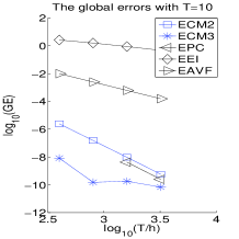
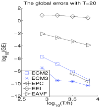
Figure 1: The logarithm of the global error against the logarithm of $T/h$.

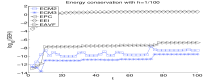
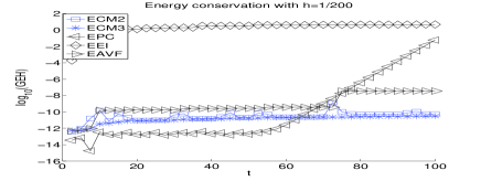
Figure 2: The logarithm of the error of Hamiltonian against $t$.

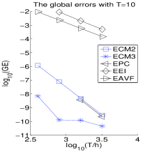
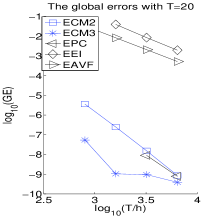
Figure 3: The logarithm of the global error against the logarithm of $T/h$.

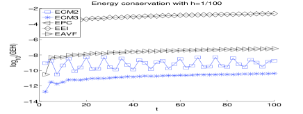
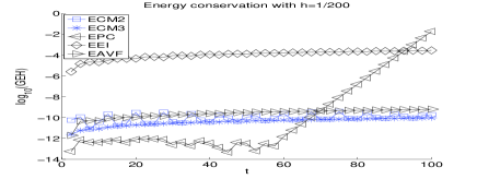
Figure 4: The logarithm of the error of Hamiltonian against $t$.

9 Conclusions

We have presented and analysed exponential collocation methods for the cubic Schrödinge Cauchy problem, which exactly or nearly preserve the continuous energy of the original system and can be of arbitrarily high order. We have also analysed in detail the properties of the new methods including existence and uniqueness, global convergence, and nonlinear stability. Furthermore, the remarkable efficiency of the methods was demonstrated by the numerical experiments in comparison with existing numerical schemes appeared in the literature. The application of the methodology for the cubic Schrödinger equation (1) stated in this paper to other Hamiltonian PDEs will be our future work in the near future.

References

[1] Ablowitz, M. J., Segur, H. Solitons and the Inverse Scattering
Transform. Society for Industrial and Applied Mathematics.
Philadelphia (1981)
[2] Akhmediev, N., Ankiewicz, A.
Taki M. Waves that appear from nowhere and disappear without a
trace. Phys. Lett. A 373: 675–678 (2009)
[3] Benetazzo, A., Barbariol, F.,
Bergamasco, F., Torsello, A., Carniel, S., Sclavo, M. Observation
of extreme sea waves in a space-time ensemble. J. Phys. Ocea. 45:
2261–2275 (2015)
[4] Cohen, D., Gauckler, L. One-stage exponential integrators for
nonlinear Schrödinger equations over long times. BIT 52:
877–903 (2012)
[5]Gauckler, L., Lubich, C. Nonlinear Schrödinger
equations and their spectral semi-discretizations over long times.
Found. Comput. Math. 10: 141-169 (2010)
[6]Gauckler, L., Lubich, C.
Splitting integrators for nonlinear Schrödinger equations over
long times. Found. Comput. Math. 10: 275–302 (2010)
[7] Agrawal, G. P. Nonlinear fiber optics, Fourth edition. Elsevier
Books, Oxford (2006)
[8]
Faou, E. Geometric Numerical Integration and Schrödinger
Equations. European Math. Soc. Publishing House, Zürich (2012)
[9] Jin, S., Markowich, P., Sparber, C. Mathematical and computational
methods for semiclassical Schrödinger equations. Acta Numer. 20:
121–210 (2011)
[10] Lubich, C. From quantum to classical molecular dynamics: reduced
models and numerical analysis. European Mathematical Society (2008)
[11] Sulem, C., Sulem, P.-L. The nonlinear Schrödinger equation. Self-focusing and wave
collapse. Applied Mathematical Sciences. 139. Springer-Verlag, New
York (1999)
[12] Bader, P., Iserles, A., Kropielnicka, K., Singh, P. Effective
approximation for the linear time-dependent Schrödinger
equation. Found. Comput. Math. 14: 689–720 (2014)
[13] Besse, C., Bidégaray, B., Descombes, S. Order estimates in time
of splitting methods for the nonlinear Schrödinger equation.
SIAM J. Numer. Anal. 40: 26–40 (2002)
[14]
Eilinghoff, J., Schnaubelt, R., Schratz, K. Fractional error estimates
of splitting schemes for the nonlinear Schrödinger equation. J.
Math. Anal. Appl. 442: 740–760 (2016)
[15]
Lubich, C. On splitting methods for Schrödinger-Poisson and
cubic nonlinear Schrödinger equations. Math. Comp. 77:
2141–2153 (2008)
[16] McLachlan, R. I., Quispel, G. R. W. Splitting methods. Acta
Numer. 11: 341–434 (2002)
[17]
Thalhammer, M. Convergence analysis of high-order time-splitting
pseudo-spectral methods for nonlinear Schrödinger equations.
SIAM J. Numer. Anal. 50: 3231–3258 (2012)
[18] Cano, B., González-Pachón, A. Exponential time integration
of solitary waves of cubic Schrödinger equation. Appl. Numer.
Math. 91: 26–45 (2015)
[19] Celledoni, E., Cohen, D., Owren, B. Symmetric exponential
integrators with an application to the cubic Schrödinger
equation. Found. Comput. Math. 8: 303–317 (2008)
[20] Dujardin, G. Exponential Runge-Kutta methods for the
Schrödinger equation. Appl. Numer. Math. 59: 1839–1857 (2009)
[21]
Ostermann, A., Schratz, K. Low regularity exponential-type
integrators for semilinear Schrödinger equations. Found. Comput.
Math. 16: 1–25 (2017)
[22] Berland, H., Islas, A. L., Schober, C. M. Conservation of phase
space properties using exponential integrators on the cubic
Schrödinger equation. J. Comput. Phys. 255: 284–299 (2007)
[23] Reich, S. Multi-symplectic Runge-Kutta collocation methods for
Hamiltonian wave equations. J. Comput. Phys. 157: 473–499 (2000)
[24] Bejenaru, I., Tao, T., Sharp well-posedness and ill-posedness
results for a quadratic non-linear Schrödinger equation. J.
Funct. Anal. 233: 228–259 (2006)
[25]
Germain, P., Masmoudi, N., Shatah, J. Global solutions for 3D
quadratic Schrödinger equations. Int. Math. Res. Notices 3:
414–432 (2009)
[26] Islas, A. L., Karpeev, D. A., Schober, C. M. Geometric integrators for the nonlinear Schrödinger
equation. J. Comput. Phys. 173: 116–148 (2001)
[27]
Kishimoto, N. Low-regularity bilinear estimates for a quadratic
nonlinear Schrödinger equation. J. Diff. Equa. 247:
1397-1439 (2009)
[28] Feng, K., Qin, M. The symplectic methods for the computation of Hamiltonian equations,
Numerical Methods for Partial Differential Equations. Springer,
Berlin 1–37 (2006)
[29] Hairer, E., Lubich, C., Wanner G. Geometric Numerical
Integration: Structure-Preserving Algorithms for Ordinary
Differential Equations. 2nd edn. Springer-Verlag, Berlin (2006)
[32]Wang, B., Meng, F.,
Fang, Y. Efficient implementation of RKN-type Fourier collocation methods
for second-order differential equations. Appl. Numer. Math. 119: 164–178 (2017)
[33]Wang, B., Wu, X., Meng, F. Trigonometric collocation methods based
on Lagrange basis polynomials for multi-frequency oscillatory
second-order differential equations.
J. Comput. Appl. Math. 313: 185–201 (2017)
[34] Wu, X., Liu, K., Shi, W.Structure-Preserving Algorithms for Oscillatory Differential Equations II.
Springer-Verlag, Heidelberg (2015)
[35]Wu, X., You, X., Wang, B. Structure-preserving algorithms for oscillatory
differential equations. Springer-Verlag, Berlin (2013)
[36] Ŝolin, P. Partial differential equations and the finite element
method. Wiley-Interscience. (2006)
[37] Dahlby, M., Owren, B. A general framework for deriving integral
preserving numerical methods for PDEs. SIAM J. Sci. Comput. 33:
2318–2340 (2011)
[38] Wang, B., Wu, X. The formulation and analysis of energy-preserving schemes for solving high-dimensional nonlinear Klein-Gordon
equations. IMA. J. Numer. Anal. DOI: 10.1093/imanum/dry047 (2018)
[39] Celledoni, E., Grimm, V., McLachlan, R. I., McLaren, D. I., O’Neale, D.,
Owren, B., Quispel, G. R. W. Preserving energy resp. dissipation
in numerical PDEs using the “Average Vector Field” method. J.
Comput. Phys. 231: 6770–6789 (2012)
[40] Brugnano, L., Frasca Caccia, G., Iavernaro, F. Energy conservation
issues in the numerical solution of the semilinear wave equation.
Appl. Math. Comput. 270: 842–870 (2015)
[41] Brugnano, L., Zhang, C., Li, D. A class of energy-conserving
Hamiltonian boundary value methods for nonlinear Schrödinger
equation with wave operator. Commun. Nonl. Sci. Numer. Simulat. 60:
33–49 (2018)
[42] Liu, C., Wu, X. An energy-preserving and symmetric scheme for nonlinear Hamiltonian wave
equations. J. Math. Anal. Appl. 440: 167–182 (2016)
[43] Liu, C., Wu, X. The boundness of the operator-valued functions for
multidimensional nonlinear wave equations with applications. Appl.
Math. Lett. 74: 60–67 (2017)
[44] Bridges, T. J., Reich, S. Numerical methods for Hamiltonian PDEs. J.
Phys. A: Math. Gen. 39: 5287–5320 (2006)
[45]Cohen, D., Hairer, E., Lubich, C. Conservation of energy,
momentum and actions in numerical discretizations of nonlinear wave
equations. Numer. Math. 110: 113–143 (2008)
[46] Diaz, J., Grote, M. J. Energy conserving explicit local timestepping
for second-order wave equations. SIAM J. Sci. Comput. 31: 1985-2014
(2007)
[47]Li, Y.W., Wu, X. General local energy-preserving
integrators for solving multi-symplectic Hamiltonian PDEs. J.
Comput. Phys. 301: 141-166 (2015)
[48] Liu, C., Iserles, A.,
Wu, X. Symmetric and arbitrarily high-order Birkhoff–Hermite time
integrators and their long-time behaviour for solving nonlinear
Klein–Gordon equations. J. Comput. Phys. 356: 1–30 (2018)
[49] Matsuo, T., Yamaguchi, H. An energy-conserving Galerkin scheme for
a class of nonlinear dispersive equations. J. Comput. Phys. 228:
4346–4358 (2009)
[50]Mei, L., Liu, C., Wu, X. An
essential extension of the finite-energy condition for extended
Runge–Kutta–Nyström integrators when applied to nonlinear
wave equations. Commun. Comput. Phys. 22: 742–764 (2017)
[51]
Sanz-Serna, J.M. Modified impulse methods for highly oscillatory
differential equations. SIAM J. Numer. Anal. 46: 1040–1059 (2008)
[52] Hochbruck, M., Ostermann, A. Explicit
exponential Runge–Kutta methods for semilineal parabolic problems.
SIAM J. Numer. Anal. 43: 1069–1090 (2005)
[53] Hochbruck, M., Ostermann, A. Exponential
integrators. Acta Numer. 19: 209–286 (2010)
[54] Hochbruck, M., Ostermann, A.,
Schweitzer, J. Exponential rosenbrock-type methods. SIAM J. Numer.
Anal. 47: 786–803 (2009)
[55] Mei, L., Wu, X. Symplectic
exponential Runge-Kutta methods for solving nonlinear Hamiltonian
systems. J. Comput. Phys. 338: 567–584 (2017)
[56] Alinhac, A., Gérard, P. Opérateurs pseudo-différentiels et théorie de Nash-Moser.
Interéditions/éditions du CNRS (1991)
[57] Hairer, E. Energy-preserving variant of collocation
methods.
J. Numer. Anal. Ind. Appl. Math. 5: 73–84 (2010)
[58] Iavernaro, F., Trigiante, D.
High-order symmetric schemes for the energy conservation of
polynomial Hamiltonian problems. J. Numer. Anal. Ind. Appl. Math.
4: 87–101 (2009)
[59] Li, Y.W., Wu, X. Exponential integrators preserving
first integrals or Lyapunov functions for conservative or
dissipative systems. SIAM J. Sci. Comput. 38: 1876–1895 (2016)
[60] Berland, H., Skaflestad, B., Wright W. M. EXPINT A MATLAB
package for exponential integrators. ACM Trans. Math. Softw. 33: (1)
(2007)