Crossroads of the mesoscale circulation.

Abstract

Quantifying the mechanisms of tracer dispersion in the ocean remains a central question in oceanography, for problems ranging from nutrient delivery to phytoplankton, to the early detection of contaminants. Until now, most of the analysis has been based on Lagrangian concepts of transport, often focusing on the identification of features that minimize fluid exchange among regions, or more recently, on network tools which focus instead on connectivity and transport pathways. Neither of these approaches, however, allows us to rank the geographical sites of major water passage, and at the same time, to select them so that they monitor waters coming from separate parts of the ocean. These are instead key criteria when deploying an observing network. Here we address this issue by estimating at any point the extent of the ocean surface which transits through it in a given time window. With such information we are able to rank the sites with major fluxes that intercept waters originating from different regions. We show that this allows us to optimize an observing network, where a set of sampling sites can be chosen for monitoring the largest flux of water dispersing out of a given region. When the analysis is performed backward in time, this method allows us to identify the major sources which feed a target region. The method is first applied to a minimalistic model of a mesoscale eddy field, and then to realistic satellite-derived ocean currents in the Kerguelen area. In this region we identify the optimal location of fixed stations capable of intercepting the trajectories of 43 surface drifters, along with statistics on the temporal persistence of the stations determined in this way. We then identify possible hotspots of micro-nutrient enrichment for the recurrent spring phytoplanktonic bloom occuring here. Promising applications to other fields, such as larval connectivity, marine spatial planning or contaminant detection, are then discussed.

1 Introduction

Suppose that a contaminant is released in a region of the open ocean. Where should a set of monitoring stations must be deployed to maximize the chances of detecting and eventually restricting the contaminant spill? Characterizing the evolution of tracers dispersed by the oceanic currents is indeed a central question in several areas of oceanography. In some cases it is possible to partially address this point by tracking a given tracer using satellite images or model simulations, but often in situ measurements and adaptive sampling strategies are required.

Relevant examples range from the retrieval of contaminants and their basins of attraction (Vrana et al., 2005; Froyland et al., 2014), larval dispersal and marine populations connectivity (Carreras et al., 2017; Bradbury et al., 2008; Planes et al., 2009; Andrello et al., 2013; Melià et al., 2016; Monroy et al., 2017), the planning of oceanographic surveys (Bellingham and Willcox, 1996), monitoring systems design (Mooers et al., 2005; de Jonge et al., 2006; Muñoz et al., 2015), to the characterization of Marine Protected Areas (Cowen et al., 2006; Siegel et al., 2008; Shanks, 2009; Rossi et al., 2014; Dubois et al., 2016; Bray et al., 2017), or to the so called Marine Spatial Planning (MSP, Viikmäe et al., 2011; Delpeche-Ellmann and Soomere, 2013a ; Ehler, 2018) which integrates all the above.

Horizontal transport at the ocean surface is one of the key mechanisms controlling the dispersion of tracers, in particular on scales of the order of days to weeks. In this time frame, a heuristic but very common assumption is that vertical velocities are weak enough so that the motion of a water parcel can be considered two-dimensional. Strictly speaking, horizontal transport affects any advected tracer through two main processes: mixing, which reduces and smooths the gradients, and horizontal stirring, which instead enhances the tracer gradients (Eckart, 1948; Okubo, 1978; Garrett, 1983; Sundermeyer and Price, 1998). Horizontal stirring is one of the main mechanism for which an initial homogeneous water mass is stretched by the currents and deformed into elongated and convoluted filaments. These features can intrude into some regions far apart from their origin, while other areas close to the source location may be shielded by circulation features, the so-called transport barriers. This filamentation process eventually enhances mixing by creating longer contact surfaces between water masses of contrasting properties.

Several tools have been proposed to achieve a better understanding of the role horizontal transport plays in tracer dispersion. Most of these approaches focus on the Lagrangian analysis of the ocean currents based on dynamical system theory (Ottino, 1989; Haller and Yuan, 2000; Mancho et al., 2004; Shadden et al., 2005; Wiggins, 2005). These methods are mainly devoted to the detection of barriers to transport in flow systems (Boffetta et al., 2001; Abraham and Bowen, 2002; d’Ovidio et al., 2004; Beron-Vera et al., 2008; Prants et al., 2014a ; Prants et al., 2014b ) or coherent regions (Lehahn et al., 2007; Froyland et al., 2007; d’Ovidio et al., 2013; Berline et al., 2014; Hadjighasem et al., 2016; Miron et al., 2017) with minimal leaking to surrounding water masses. Interestingly, during the last years, network theory approaches to geophysics (Phillips et al., 2015), flow transport and mixing (Ser-Giacomi et al., 2015a ; Lindner and Donner, 2017; Fujiwara et al., 2017; Molkenthin et al., 2017; Padberg-Gehle and Schneide, 2017; Ser-Giacomi et al., 2017; McAdam and van Sebille, 2018), and turbulence (Iacobello et al., 2018; Gopalakrishnan Meena et al., 2018) have also attracted lot of interest.

Recently, more attention has been given to a problem that is complementary and somehow opposite to the identification of transport barriers: how to detect regions that enhance fluid exchanges across a flow system (Ser-Giacomi et al., 2015b ; Ser-Giacomi et al., 2015c ; Costa et al., 2017; Lindner and Donner, 2017; Rodríguez-Méndez et al., 2017; Koltai and Renger, 2018)? This issue has been developed particularly in the framework of networks built from Lagrangian trajectories (Ser-Giacomi et al., 2015a ). In such studies, spatial sub-areas of the ocean are represented by network nodes while links parameterize the amount of water exchanged among them. Networks constructed in this way, called Lagrangian Flow Networks (LFNs), provide thus a topological description of the transport dynamics in the ocean allowing to describe features of the flow by using several network methods and tools.

In particular, it has been shown the existence of localized “bottlenecks”whose presence maintains connections between areas of the seascape that would be otherwise almost disconnected. Borrowing from Network Theory the concept of betweenness centrality, it has been possible to quantify explicitly how much LFN nodes act as bottlenecks for the oceanic flow by counting the number of paths passing through them during a fixed interval of time (Ser-Giacomi et al., 2015b ).

The main limitation of the betweenness centrality concept, however, is that it identifies bottleneck regions that, even if topologically relevant for the connectivity geometry, do not present necessarily an important water flux. This is related to the fact that the betweenness measures the number of connections crossing a node, regardless of connectivity strength. Therefore, to pinpoint hotspots that maximize the incoming or outgoing flux in a given time window, one should focus on strong “passage points”of water, instead of only topological bottlenecks.

In this paper we aim to detect these hotspots, which act as “crossroads”of the circulation, being traversed by the largest amount of water coming from (or going to) a focal region. This is achieved by defining a quantity, which we call crossroadness, which is the surface flow through each spot of the domain considered in a specific temporal window.

Moreover, our calculation preserves the information on the original location of each passing trajectory. Based on the crossroadness analysis, we introduce an algorithm for designing a sampling network with minimal redundancy, i.e. in which the flow of a given source region through the network is maximized and the number of stations minimized. Reversing the analysis backward in time, we can use the same method to find the major “source”points from which the water distributes over a target area. The paper is organized as follows: Sec. 2 describes the methodological framework, the theoretical model and the dataset employed for the computation and the validation of the results. In particular, Subsec. 2.1 introduces the crossroadness and its fluid dynamical and oceanographic interpretation. We then determine a ranking method (Subsec. 2.3) that provides the sites with the major passage of water dispersed from a source region or feeding a target region, when computed forward or backward in time, respectively. Validation and case studies are then described in Sec. 3. In Subsec. 3.1, we first analyse the crossroadness properties of a simple steady vortex configuration obtained from the 2D Navier Stokes equation. In Subsec. 3.2, the method is applied to satellite altimetry data and validated against the trajectories of real SVP drifters in the Southern Ocean. In Subsec. 3.3, the relationship between the surface being monitored and the number of stations employed is examined. An analysis of the persistence of the observing network is reported in Subsec. 3.4. In Subsec. 3.5, we use the method to identify possible sites from which nutrients are delivered offshore the Kerguelen plateau, fuelling the open ocean planktonic bloom. A summary of the results, along with an illustration of the perspectives and possible fields of application is given in the Discussion (Sec. 4). Finally, our paper is completed by two appendices, extending the analysis of the sensitivity of our diagnostic to changes in the dates of the velocity field used (Appendix A), and giving some demonstration of the link of our new diagnostic, under particular hypotheses, to averages of velocity and of kinetic energy (Appendix B).

Figure 1: Illustrative example for the calculation of the crossroadness. Colored dotted lines correspond to different trajectories originating from the initialization grid (left), advected for a time $\uptau$. The circle (thick dotted line) represents the detection range of the station of the observational grid (right), while the rectangles (thin dotted line) contain the surface of water that passes through the station.

2 Data and Methods

2.1 The crossroadness: characterizing regions by the amount of water crossing them

We define a new metric, that we call crossroadness (CR), measuring the surface crossing a region of a given size in a fixed temporal window.

To do this, we consider two grids, the initialization and the observational grid (Fig. 1), of cell sizes $\delta_{IG}$ and $\delta_{OG}$ respectively, where each cell is represented by its central point. If $\delta_{IG}$ is small enough, we can consider every central point as representative of the content of the cell.

Each central point of the initialization grid is advected and defines a trajectory. The observational grid represents instead the domain over which we compute the crossroadness (see also Subsec. 2.7). For each point $\mathcal{P}$ of this grid, we count the number of trajectories passing below a distance $\sigma$ from $\mathcal{P}$. This is done by computing the Euclidian (or spherical when working with spherical coordinates) distance between $\mathcal{P}$ and the first point of the trajectory, then the second one, the third one and so on. We obtain thus $N_{PT}$ values. We consider as distance between the trajectory and $\mathcal{P}$ the minimum among the $N_{PT}$ values. $\sigma$ represents the neighborhood radius (the detection range) of each point in the observational grid. In spherical coordinates, if $\sigma$ is given in radians, this radius is indeed $R\sigma$. As the dimensions of a cell in the initialization grid are relatively small, we can consider that the trajectory is representative for the whole content of the cell from which it is originated (therefore, $\sigma\geq\delta_{IG}$). Thus, if we multiply the number of trajectories counted times the surface of an initialization cell, $\Delta$, we will obtain an estimation of the total water surface that passed through the node during the period $\uptau$. We call this total water surface flowing inside the detection range of the point $\mathcal{P}$ the “crossroadness”(“CR”) at $\mathcal{P}$. In this way we define a CR field on all points of the observational grid. A representative scheme of this concept is illustrated in Fig. 1, where the crossroadness of the point in the circle is $3\Delta$ since there are three trajectories entering its detection range. Because of the quasi-twodimensional nature of ocean circulation at the scales considered here, the amount of surface is proportional to the volume and then to the mass of the water transported in the upper ocean layers. The same procedure can be applied backwards: the initialization grid is advected backward in time, and, over the observational grid, we count for each point how many trajectories pass closer than the detection range $\sigma$. In this way we obtain the crossroadness field backwards in time.

2.2 Theoretical relation of the crossroadness with absolute velocity and mean kinetic energy

Intuitively, one can expect higher crossroadness values in points where the velocity is higher, because the corresponding particle fluxes are also larger. The situation is in fact more complex because a map of crossroadness is associated only to the trajectories stemming from a specific region. It is however instructive to study the case in which the trajectories stem from the entire domain (i.e., when the initialization grid coincides with the observational grid), because in this case the crossroadness has a direct proportionality relation with the kinetic energy.

To show this relation, we note that every circle of radius $\sigma$ around an observational station presents a cross section (more properly a cross-length) $2\sigma$ perpendicular to the flow coming from any direction. If $\sigma$ is sufficiently small to allow considering the velocity field constant on the whole observational circle, the amount of surface crossing that station in a short interval of time $dt$ is $2\sigma|v|dt$, with $|v|$ the velocity modulus at the station. Integrating during a time $\uptau$ we find that the CR at that point can be written as

$$CR=\int_{D_{0}}^{D_{0}+\uptau}2\sigma|v|dt=2\sigma\uptau<|v|>\ ,$$ (1)

with $<|v|>$ the temporal average of the speed $|v|$ in the time interval $\uptau$. If the temporal fluctuations of $|v|$ during the time interval $\uptau$ can be neglected, i.e. $<v^{2}>\approx<|v|>^{2}$ then a relationship with the temporal average of the kinetic energy per unit of mass of the flow, $<E_{K}>=<v^{2}/2>$, would hold:

$$CR\approx 2\sigma\uptau\sqrt{2<E_{K}>}.$$ (2)

The formulas above present the announced approximate relationship between the crossroadness and the flow speed. For a validation of Eq. (1) and (2), please refer to Appendix B.

As we shall see, more complex crossroadness patterns arise when the trajectories do not originated from the entire domain.

2.3 Ranking method for the optimization of a network of CR stations

Figure 2: Illustrative scheme for the determination of the position of a network of observing stations which maximize the detection of a dispersed tracer. The first station is the one that collects the largest number of trajectories, in this case the one circled in the left panel (4 trajectories). Then, we have 3 possible second stations, each with 3 trajectories passing near them (middle panel). But since we consider only independent trajectories, we have to exclude the ones already sampled by the first station (panel on the right). In this way we have only one second possible station.

In the study of the dispersion of a passive tracer one of the main questions is the definition of an effective sampling strategy. Considering the tracer (e.g. a contaminant) with a finite life time, we want to know what would be the best distribution of monitoring sites (referred to as “stations”) that can intercept the largest fraction of the advected tracer. In a turbulent pattern of circulation, the answer to this question is not obvious, since the patch can be redistributed irregularly through the domain considered.
Sampling on a regular grid is a possible choice. However, depending on the circulation patterns, we can easily imagine that some retrieving sites may convey water from larger regions than others. The crossroadness provides implicitly a simple method for the definition of a sampling strategy. In fact, if we want to choose the best monitoring station, we will simply select the site crossed by the largest number of trajectories originated by the source region of the tracer, i.e. the one with the higher value of crossroadness. In order to define the second most important monitoring station, we exclude the trajectories already monitored by the first station. We consider only independent trajectories, i.e. originated from different locations of the initialization grid, and we determine also the second station. Proceeding iteratively in this way we identify a network of CR stations (Fig. 2).
The calculation can be performed backward in time as well. The initialization region becomes a target region. In this case, the network of CR stations represents the ensemble of locations which maximize the surface water feeding the target region.

2.4 A simple steady vortex field

We consider a numerical simulation of the Navier Stokes equation in two dimensions, which, for the scalar vorticity field $\omega=\nabla\times\textbf{u}$ of an incompressible fluid ($\nabla\cdot\textbf{u}=0$, in which u=(u,v) is the velocity field), can be written as:

$$\frac{\partial\omega}{\partial t}+\omega\cdot\nabla\textbf{u}\,=\,\nu\nabla^{2}\omega-\alpha\omega+f_{\omega}$$ (3)

in which $\nu$ is the kinematic viscosity, $-\alpha\omega$ is a friction term removing energy at large scales and $f_{\omega}$ represents a forcing term necessary to maintain a stationary state. All the quantities are adimensionalised. We use a forcing on a narrow band of wave numbers around $k_{f}$=2 in Fourier space which is constant in time and acting with a fixed phase $\theta=\pi$ . We take $\nu=0.5$, $\alpha=0.025$ and we integrate Eq. 3 with a pseudospectral code on a box of size $L_{x}=L_{y}=2\pi$ with periodic boundary conditions and 512² grid points. Starting from a null vorticity field, the model is run for 15600 steps (dt$=5\cdot 10^{-4}$, t$\,=7.8$), until the energy of the system is constant ($E=0.06$) and a steady vorticity (and velocity) field is reached. More details on the model are provided in Boffetta et al., 2002; Boffetta and Musacchio, 2010.

The stationary vorticity field obtained is in Fig. 3. It is formed by a series of anti-clockwise (in blue) and clockwise (in red) rotating vortexes. Particles, disposed on a regular grid of 256² points, are then advected using a second order Runge Kutta method as explained in Subsec 2.7. The vorticity field is considered to cover periodically the full horizontal plane, on which the particle move, although we will only display and analyze the subdomain [0,2$\pi$]$\times$[0,2$\pi$]. Finite Time Lyapunov Exponents (FTLE) forward ($\lambda^{f}$) and backward ($\lambda^{b}$) in time are computed from the trajectories, following the definition in Shadden et al., (2005).

Figure 3: Two-dimensional steady vorticity field as obtained from Eq. 3. The box size are $L_{x}=L_{y}=2\pi$ and the vorticity field was integrated with a resolution of 512² grid points regularly spaced.

2.5 Ocean satellite-derived velocity field and chlorophyl data

We focus on the Kerguelen region of the Southern Ocean, where in 2011 the KEOPS2 campaign released, over 20 days, a set of 48 Surface Velocity Program (SVP) drifters. We use a set of stations, defined by our method, for a virtual “search and rescue”of these drifters. For their computation, we use satellite-derived velocity fields, which are obtained through the geostrophic approximation from the measurement of the Sea Surface Height (SSH). This approximation and the relatively low spatial and temporal resolution of satellite products often risk to smooth mesoscale structures (Bouffard et al., 2014), especially close to the coast (Nencioli et al., 2011). The comparison between satellite-derived crossroadness and real drifter trajectories is thus a realistic assessment of the capacity of the algorithm described here to identify points with enhanced passage of particle trajectories.

The Kerguelen region is also characterized by a massive spring-time phytoplanktonic bloom, extended for hundreds of kilometres, preconditioned by the redistribution of micro-nutrients (in particular iron) advected by the Antarctic Circumpolar Current (ACC) from the Kerguelen plateau margin out into the open ocean (d’Ovidio et al., 2015). Satellite-derived chlorophyll is therefore a useful tracer of transport pathways, and an opportunity for pinpointing likely sources of iron by employing the theoretical concepts developed in this paper.

For the velocity field we use the DUACS (Data Unification and Altimeter Combination System) delayed-time multi-mission altimeter gridded products defined over the global ocean with a regular $\frac{1}{4}\times\frac{1}{4}\degree$ spatial sampling (Pujol et al., 2016) and available from the E.U. Copernicus Marine Environment Monitoring Service (CMEMS, http://marine.copernicus.eu/). An experimental product, which used an improved mean dynamic topography and for which the altimetric tracks have been interpolated with optimized parameters, is also considered. It corresponds to the AVISO regional Kerguelen product, velocities computed from altimetry in delayed time on a (higher resolution) $\frac{1}{8}\times\frac{1}{8}\degree$ regular grid (http://www.aviso.altimetry.fr/duacs/).

The field of chlorophyll was downloaded from the Oceancolour product (OCEANCOLOUR_GLO_CHL_L4_REP_OBSERVATIONS_009_082) at CMEMS. These data are provided by a map computed from satellite observations over a period of 8 days (to limit cloud coverage), and with a spatial resolution of $4$ km$\times\,4$km.

2.6 SVP drifters

During the KEOPS2 campaign in October-November 2011, 48 Surface Velocity Program (SVP) drifters were released within the Kerguelen region. The SVP drifting buoy is a Lagrangian current-following drifter, composed of a spherical surface float of 35 cm in diameter, which contains the battery, a holey sock drogue of about 6 meters that tracked the water currents at a nominal depth of 15 m, representative of the surface circulation, and a satellite transmitter which relays the data through the Iridium system. All the buoys address the World Ocean Circulation Experiment (WOCE) benchmarks.

In our study we consider only the drifters released on the eastern part of the Kerguelen plateau, i.e. at a longitude greater than $68\degree$E. We therefore consider 43 drifters trajectories of the 48 drifting buoys originally deployed. We assume the 11th of November 2011 as the release date. The duration of the trajectories ranges between 63 to 93 days (average of 81 days), with a temporal resolution of 1 day.

2.7 Initialization and observational grids

We describe here the details of the construction of the two grids used for the computation of the crossroadness.

For the Navier Stokes model, particles start over an initialization grid of 256² regularly displaced points ($\delta_{IG}=0.0246$) and are advected with a second order Runge-Kutta scheme for a period t=11.7, corresponding to 23400 steps.

When working with altimetric velocities, the points of the initialization grid are advected using DUACS altimetric velocities with a 4th order Runge-Kutta integration scheme, for a period between 30 and 90 days and a time step of 3 hours. Each trajectory thus computed contains 8 points per day ($N_{PT}\,=\,8\,N_{D}$ in total, $N_{D}$ number of days). We remind that the period of integration is chosen so that the vertical motion can be neglected. Indeed, below 2-3 months, and excluding some peculiar regions of convection, the vertical velocity is usually 2$\sim$3 orders of magnitude smaller than the horizontal one, and thus the ocean surface motion can be approximated as two dimensional (d’Ovidio et al., 2004; Rossi et al., 2014).

We note here that, when working with altimetric velocities, and thus in spherical coordinates, we impose that all the cells have the same size. The initial angular separation between two contiguous particles ($\delta_{IG}$) used in the computations varies from 0.1 to 0.4 degrees. By initial separation $\delta_{IG}$ we mean the difference in latitude among contiguous rows of particles. Along the longitudinal (LON) direction, to keep the same distance, the separation is thus corrected by the cosine of the latitude LAT ($\delta_{LON}=\delta_{IG}/\cos(LAT)$). In this way all the cells have the same lateral sizes, $R\delta_{IG}$, and area $\Delta=R^{2}\delta_{IG}^{2}$ (with $\delta_{IG}$ in radians, and $R$ the Earth radius). The observational grid in spherical coordinates is built in the same way as the initialization grid.

In Sec. 3 we will always refer to them as initialization or observational grid, but keeping in mind their difference (for Navier Stokes and altimetric velocities) in Euclidian and spherical coordinates.

3 Results

3.1 The crossroadness in the steady Navier-Stokes 2D vortex configuration

To gain some insights on the interpretation of the crossroadness and on its differences in respect to other Lagrangian methods, we present here the analysis of the flow associated to the vorticity field shown in Fig. 3, obtained from the numerical simulation of Eq. (3), as explained in Subsec. 2.4. The flow contains 4 vortices rotating clockwise (positive vorticity, red patches) and a central vortex rotating anti clockwise (in blue). 9 other anti clockwise rotating vortices are present partially on the edges of the box. The vortices are surrounded by separatrices made of the stable and unstable manifolds of fixed hyperbolic points, arranged in a square lattice. To visualize these separatrices we compute in Fig. 4 Finite Time Lyapunov Exponent fields (FTLE, defined as in Shadden et al., 2005). Forward ($\lambda^{f}$) and backwards ($\lambda^{b}$) FTLE are calculated for an integration time $\tau=\pm 11.7$ on a grid of 256² points, and we plot their sum. The ridges of such field clearly identify the stable and unstable manifolds and its maxima highlight the position of the correspondent hyperbolic points.

As a first step, we compute the crossroadness field and the associated monitoring stations considering as initialization grid 256² particles regularly displaced on the entire domain ($\delta_{IG}=0.0246$). The observational grid is made of 128² points ($\delta_{OG}=0.0490$). Particles in the initialization grid are advected forward in time for t$=11.7$, i.e. the same period considered for the computation of the FTLE of Fig. 4A. Finally, we consider as detection range $\sigma=0.1$. The result is shown in Fig. 4B. The crossroadness pattern in itself does not contain much valuable information, because (as explained in Subsec. 2.2) when the initialization grid covers the entire domain the crossroadness closely matches the kinetic energy (except for points very close to the border). The position of the monitoring stations selected by the ranking algorithm (the set of points crossed by the largest number of independent trajectories) however is not trivial. They are shown as black dots in each panel. For the first five, we plotted also their detection range and order of importance (white number inside the circle). Although in general FTLE ridges have large crossroadness values, only the first two stations (white numbers 1 and 2) fall over a manifold. This fact can be understood noting that multiple stations over the manifolds would be redundant, because they would sample trajectories intercepted by other stations. Interestingly, 173 stations were found to be necessary in order to sample the whole region. Multiplying this value for the surface of a station, i.e. $\pi\sigma^{2}$, we obtain that they cover only 14$\%$ of the total box surface. When considering instead a $\sigma=\delta_{OG}$, 632 stations, covering just the 3$\%$ of the total surface, were needed to sample the whole region.

We then changed the initialization grid, considering all the particles belonging to an ellipse of center $x_{C}=\pi$, $y_{C}=\frac{3}{2}\pi$, with semi-axes $r_{x}=1$, $r_{y}=0.5$. We note that the ellipse is thus centered exactly over a hyperbolic point. Finally, $\sigma$ is set to 0.3. The results are reported in Fig. 4C-D. Contrary to the previous case, The pattern of the crossroadness is intimately linked to the choice of the initialization grid and also to the direction of the advection (forward or backward).

Figure 4: Panel A: Forward ($\lambda^{f}$) and backwards ($\lambda^{b}$) FTLE fields, computed with integration times $t=\pm 11.7$ respectively, and over a 256² regular grid. They identify the locations of stable and unstable manifolds and the associated hyperbolic points. The quantity actually plotted is $\lambda^{f}+\lambda^{b}$ Panel B: crossroadness forward in time, obtained from the advection of a 256² regular initialization grid (covering the whole domain) for a time $t=11.7$, computed over a 128² observational grid covering the same domain. $\sigma=0.1$. Panel C-D: crossroadness, forward and backward in time respectively, computed from the advection of the points started at the ellipse (black dotted line) centered in $x_{C}=\pi$, $y_{C}=\frac{3}{2}\pi$, with semi-axes $r_{x}=1$, $r_{y}=0.5$ and spatial separation between two contiguous particles $\delta_{IG}=0.0246$, for a time $t=\pm 11.7$, respectively. The observational grid is the same of panel B. For B,C,D, each black dot represents a CR station. The detection range of each of the 5 most important stations is displayed as a black circle, and contains the order of priority of each station (white number).

Looking at the disposition of the CR stations for the backward-in-time case it is possible to note that the first two stations are situated over the regions of highest crossroadness, and in symmetric positions in respect to the starting ellipse (dotted line). However, they do not fall exactly on the manifolds. The subsequent stations are not displaced symmetrically, and their disposition does not appear obvious. For instance, the 3rd station is on a branch of the crossroadness pattern far away from the ellipse and, interestingly, does not fall in any of the two regions with relatively high values of CR (the one at $x\simeq 5$, $y\simeq 4$ and the other at $x\simeq 1$, $y\simeq 5.5$). As in the previous case, this is due to the fact that the fluxes passing there have already been intercepted by the first two stations. The 4th station, instead, falls almost totally inside the starting ellipse. Finally, the last station (not numbered) falls in a region of higher crossroadness than the previous three.

3.2 SVP drifters and crossroadness in the Kerguelen region

Figure 5: Trajectories of the 43 drifters of the KEOPS2 Campaign. Black dots represent the starting positions of the drifters.

In order to test the crossroadness and the ranking method as defined in Subsec. 2.1 and 2.3 in a real oceanic environment, we use the dataset from the KEOPS2 campaign, in which 43 drifters were released in a relatively small area (the eastern margin of the Kerguelen plateau), approximately in the same period of time (around the 11th of November 2011), and advected for a similar window of time ($\uptau_{D}=81$ days on average) by the currents, as shown in Fig. 5. We use thus 43 real drifter trajectories.

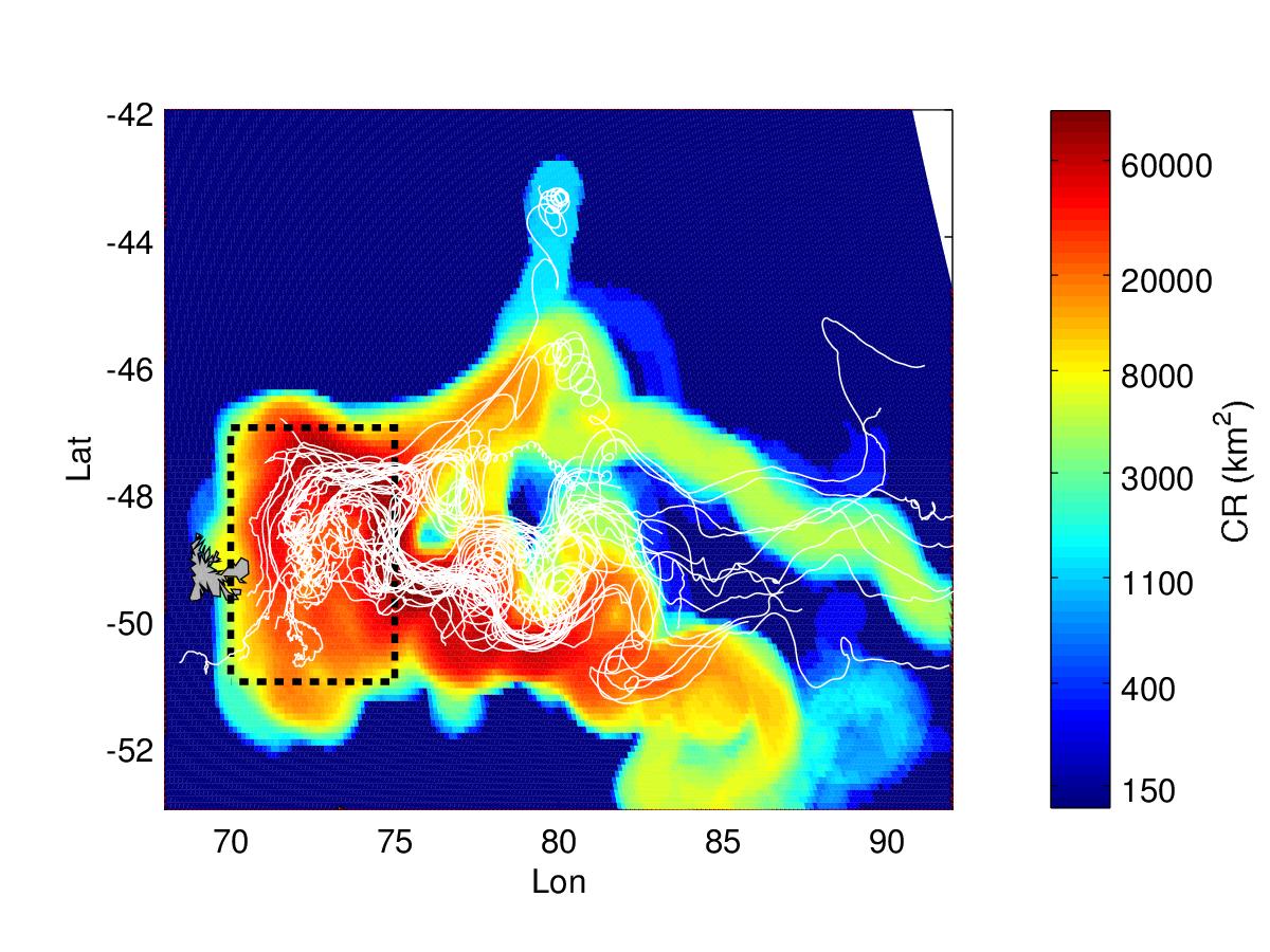
Figure 6: Crossroadness field derived from satellite altimetry ($\uptau=60$ days, $\delta_{IG}=\delta_{OG}=0.1\degree$, $\sigma=0.4\degree$), with superimposed trajectories of SVP drifters released during the 2011 KEOPS2 campaign. The CR field was computed advecting only the small rectangle (longitude: [70, 75]$\degree$; latitude: [-51, -47]$\degree$, black dotted line) in which the drifters have been released.

Figure 7: Left panel: first 6 CR stations (black stars) superimposed on the CR field computed advecting the same region as in Fig. 6, using the regional product for the velocity field ($\uptau=60$ days, $\delta_{IG}=\delta_{OG}=0.1\degree$, $\sigma=0.2\degree$). Right panel: same CR field, this time the black stars identify 6 stations disposed on a regular grid. For each station, the first number identifies the amount of total drifters intercepted, the value in brackets the number of independent drifters. Amount of drifters intercepted by the CR stations (total and in parenthesis the independent): 69 (38). Regular grid: 28 (22).

Our aim is to compare the regions of densest passage of these real buoys with the ones predicted by the CR method, which is based on oceanic currents estimated from satellite altimetry. Therefore, the initialization grid consists in a series of virtual drifters displaced in the following way: we consider the region of release of the real drifters (between [-51, -47]$\degree$S, and [70, 75]$\degree$E). We cover it with rows of virtual tracers, separated by $\delta_{IG}=0.1\degree$ along the latitude. In order to preserve the same angular distance (0.1$\degree$) among tracers of the same row, we make a latitudinal correction on their longitudinal separation, so that $\delta_{LON}=\delta_{IG}/\cos(LAT(row))$, as explained in Subsec 2.1. We put in each row the same number of virtual drifters. Thus, the longitude range of the southern row (at latitude 51$\degree$S) is [70,75.4]$\degree$. For simplicity we will denote in the following this type of geographic region as a rectangle of coordinates longitude=[70, 75]$\degree$ and latitude=[-51, -47]$\degree$.
We use the altimetry-derived velocities to advect these points forward in time for a period of $\uptau=60$ days, comparable with $\uptau_{D}$. We compute the CR values at all points separated by the same distance $\delta_{IG}$ on the Kerguelen region, i.e. a rectangle of boundaries longitude=[68, 92]$\degree$ and latitude=[-53, -42]$\degree$, which constitutes our observational grid. The resulting CR field is displayed in Fig. 6. We see a remarkably good agreement between features in the drifters trajectories and the ones in the CR field: areas of denser buoy passage correspond with higher values of the field, suggesting a good qualitative match between CR high values and areas of drifters passage.

Drifters Intercepted

CR Stations Global product Regional product Grid $\sigma$=0.1° 30.5(25.5) 30.0(23.5) 12.0(11.0) $\sigma$=0.2° 53.0(34.0) 68.3(37.3) 28.0(22.0) Total mean 41.2(30.6) 51.0(31.8) 21.6(17.6)

Table 1: Number of drifters intercepted (out of 43) using six CR stations (left columns) or six stations disposed on a $3\times 2$ regular grid. The value is an average obtained changing the different parameters used (the advection time $\uptau$, the detection range $\sigma$ and the resolution of the initialization and observational grids $\delta_{IG}$and $\delta_{OG}$, which were kept equal). For each cell, the two values correspond respectively to the total number of drifters intercepted by the stations and, in parenthesis, to the independent ones. First column: global product for altimetric velocities. Second column: regional product. Third column: stations on a regular grid.

More quantitative results are obtained by considering a set of 6 best-ranked CR stations (the choice on the quantity of stations is arbitrary) with the method explained in the previous section. The number of real drifters intercepted by the CR stations is compared to the result obtained by a set of stations placed on a regular grid. This last set is constituted by $3\times 2$ stations distributed over the area of the drifters motion, separated longitudinally by $2.5\degree$ and $1.23\degree$ latitudinally.
The measure is repeated several times and for different parameters, changing the advection time $\uptau$ (at 30, 60 and 90 days), the detection range $\sigma$ (at $0.1$, $0.2$ and $0.4\degree$) and the resolution of the initialization and observational grids $\delta_{IG}=\delta_{OG}$ (at $0.1$ and $0.2\degree$). An illustrative example is reported in Fig. 7, where $\sigma=0.4\degree$, $\delta_{IG}=\delta_{OG}=0.1\degree$ and $\tau=60$ days.
For each station, the total number of intercepted drifters is computed, as well as the number of drifters first detected by this station (independent ones). The results are reported in Table 1. The first two columns show the number of drifters (total and independent) intercepted with the CR stations, the third one the values obtained with a regular grid. The efficiency of our method is about twice the result obtained with a regular grid. A lower value of sigma corresponds not surprisingly to a lower number of catches for both the CR and the regularly spaced observational grid, but to an improved ratio in favor of the CR network.

3.3 Dependence of the surface monitored on the number of monitoring CR stations

Figure 8: For this plot and the ones showed in Appendix A, the initialisation grid is the rectangle between longitude=[55, 100]$\degree$, latitude=[-36, -59]$\degree$, while the observational grid corresponds to the domain showed, if not specified differently. Crossroadness computed with an advection time $\uptau=60$ days, $\delta_{IG}\,=\,\delta_{OG}\,=\,\sigma=0.2\degree$, with, superimposed, the first four CR stations (white circles) and the surface that they control (black dots on the corresponding initialization grid points). Note that some black dots can be outside the plot, since we advected a larger region than the observational domain showed in the panel, in order to take into account the particles upstream.

Figure 9: Histogram, computed from 100000 experiment repetitions, of the surface detected choosing each time $N=20$ stations randomly displaced. The vertical red line on the right is instead the surface scanned choosing the stations with our CR algorithm. Here $\sigma=0.4\degree$. The distance between the mean value of the distribution (vertical blue line) and the vertical red line is 9.96 times the standard deviation of the distribution.

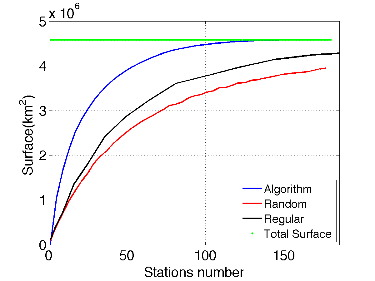
Figure 10: Surface sampled varying the number of stations considered ($\uptau=60$ days, $\delta_{IG}=\delta_{OG}=0.1\degree$, $\sigma=0.4\degree$), chosen randomly (red line), on a regular grid (black line) and with the CR method (blue line). Concerning the random choice and the regular grid, each value was obtained from the average of 1000 repeated measures. For the case of the regular grid, each time it was rigidly shifted along the longitude and the latitude of a random fraction of the distance between two grid points. The green line represents instead the total surface.

We present here a statistical analysis in order to assess the efficacy of a CR based detection network with respect to a set of stations randomly chosen or arranged on a regular grid. The benchmark that we use is the CR, i.e. the ocean surface crossing the CR observing network as a function of the number of the monitoring stations.

Figure 8 displays a map of forward crossroadness computed around Kerguelen Island, advecting particles starting from November 1st, 2011, for a time of 60 days. Superimposed, white circles identify the first four CR stations. Black dots identify the monitored waters, namely the points that will pass in proximity of one of the four stations during the advection time $\uptau$.

First, we measure the surface monitored by 20 randomly selected stations with a detection range of $0.4\degree$ in a period of 60 days. The measure is repeated $100000$ times and the results are reported in the histogram of Fig. 9. The vertical blue line is centered on the mean value of the distribution, while the red one is the value of the surface scanned with 20 stations chosen with our method. The distance between the two measures is about ten times the value of the standard deviation of the distribution, an extremely significant ($p<10^{-22}$) deviation with respect to the expected result of monitoring a larger surface with randomly selected stations.

The measure is repeated changing the number of stations selected, and the results are shown in Fig. 10. A sampling with a regular grid is performed as well. In this case, each measure is obtained by rigidly shifting the grid by a random fraction of the grid step along longitude and latitude. The use of the CR stations (blue dots) shows a better performance compared to the regular grid (black stars) and the random case (red circles) sampling. For instance, to scan a surface of $3\times 10^{6}\>km^{2}$ with a detection range of $R\sigma=40km$, 25 stations selected with the CR method are needed, about 55 with a regular grid, and 75 randomly chosen.

3.4 Persistence of the monitoring network

The calculation of the crossroadness computed in the previous sections requires that at the moment of choosing the monitoring stations, the velocity that will disperse the tracer in the future is already known with good precision. As an example, in Subsec. 3.2 we calculated the CR stations used to intercept the SVP drifters using the velocity data of the days in which the buoys were advected by the currents. How much this impacts the CR stations ability to intercept the maximal surface of a stirred patch? Here we attempt to address this question by looking at the “persistence”of the CR stations i.e. the ability of a CR network, using velocity of the past, to intercept a tracer dispersed in the near future.

Surface monitored using past velocity field for the computation of the CR stations.

In general, we define

$\mathcal{T}(\mathcal{R})_{D_{0}\rightarrow D_{f}}$

as the whole collection of trajectories $\mathcal{T}$ generated from the advection of all the points regularly initialized over a region $\mathcal{R}$, from the day $D_{0}$ until $D_{f}$. In general, from a set of trajectories $\mathcal{T}(\mathcal{R})_{D_{0}\rightarrow D_{0}+\uptau}$, we can compute an ensemble of CR stations $\mathcal{S}(\mathcal{R})_{D_{0}\rightarrow D_{0}+\uptau}$, as explained in Subsec. 2.3, that will be for construction the best choice in order to scan $\mathcal{T}$.

When the velocity field between the day $D_{0}$ and $D_{0}+\uptau$ is not known, we can use the stations computed with the velocity field in a time interval previous to $D_{0}$, e.g. $\mathcal{S}(\mathcal{R})_{D_{0}-\uptau\rightarrow D_{0}}$ to monitor the area, under the assumption that if the flow does not change much in an interval of time of the order of $\uptau$ the optimal stations will maintain approximately the same positions.

Figure 11: CR, i.e. surface monitored as a function of the number of stations. Each point is the average obtained changing $D_{0}$ over the first day of each month of 2011. Black stars represent the value obtained using the stations computed with the proper velocity field, i.e. $\mathcal{S}(\mathcal{R})_{D_{0}\rightarrow D_{0}+\uptau}$, while blue dots the ones computed with the previous $\uptau$ days, (i.e. $\mathcal{S}(\mathcal{R})_{D_{0}-\uptau\rightarrow D_{0}}$). Red circles are the values obtained with a regular disposition of the sampling sites. Left panel: $\mathcal{R}\,=\,\mathcal{R}_{P}$ (plateau region). Right panel: $\mathcal{R}\,=\,\mathcal{R}_{T}$ (turbulent area). $\delta_{IG}\,=\,\delta_{OG}\,=\,0.2\degree$, $\uptau=60\,$days, $\sigma\,=\,0.2\degree$.

Thus, in this section we use the velocities between $D_{0}-\uptau$ and $D_{0}$ to compute a set of stations $\mathcal{S}(\mathcal{R})_{D_{0}-\uptau\rightarrow D_{0}}$. We use then the latter to monitor $\mathcal{T}(\mathcal{R})_{D_{0}\rightarrow D_{0}+\uptau}$ and see how many trajectories (i.e. sea surface) they intercept.

We take as $D_{0}$ the 1st January, 2011 and $\uptau=$ 60 days. We change the number of stations considered between 1 and 16, analogously to what has been done in Subsec. 3.3. For comparative purposes, we also measure the surface intercepted with $\mathcal{S}(\mathcal{R})_{D_{0}\rightarrow D_{0}+\uptau}$, and then with a regular disposition of the stations. We then repeat the procedure using as $D_{0}$ the 1st February 2011, then the 1st March 2011 and so on, until the 1st of December 2011 and we consider the average of the 12 values obtained. In this way we obtain a more consistent statistics.

The results are reported in Fig. 11. We consider two different monitoring areas: the first one is the drifters release area, defined in Subsec. 3.2, situated mainly on the Kerguelen plateau and in which the bathymetry seems to affect the circulation pattern, making it more persistent in time. We will refer to it as $\mathcal{R}_{P}$. We then consider a more turbulent region situated offshore from Kerguelen, in which the current field should not be as constrained by the shallow shelf structures as in the former case, and in which the mesoscale structures affect deeply the variability of the currents (Park et al., 2014). We take this turbulent region $\mathcal{R}_{T}$ to be the rectangle with longitude between $80$ and $83\degree E$, and latitude between $47$ and $50\degree S$.

Concerning the plateau region (left panel in Fig. 11), we see a stronger performance of the CR stations compared to the regular grid, even if they are computed with the trajectories of two months before. E.g., in order to monitor a surface of $100000\,km^{2}$, we need 8 stations disposed regularly, while only 4 if we consider the stations obtained from the advection of the previous 60 days, and 3 if we consider the advection from time $D_{0}$ (i.e. the velocity field simultaneous to the surface advection).

The results are worse but surprisingly consistent for the turbulent region scenario (right panel in Fig. 11), with about $25\%$ less CR stations needed than in the regular case. The analysis in this section is completed in Appendix A, in which the detection power of the CR stations is assessed against further changes in the dates used for the velocity field.

3.5 Identification of a source region

In the previous section we used CR for intercepting a tracer stirred from a given region. Here instead we study another typical problem arising when studying dispersion, namely the identification of the most important source regions connected by the circulation to a given target area.

This occurs, for instance, when we aim to determine the key regions that can affect vulnerable marine protected areas downstream, or in the identification of nutrient sources feeding a biogeochemical active region (Ciappa and Costabile, 2014; Suneel et al., 2016).

In order to showcase this application, we considered the area studied in the previous section, i.e. the Kerguelen plateau, that recent studies have stressed as a natural source of iron supply that sustains the primary production in the zone situated to the east of the island (d’Ovidio et al., 2015; Blain et al., 2008; Christaki et al., 2008).

Large areas of the Earth oceans present waters with high quantities of nutrients, but low concentration of chlorophyll (HNLC). This is generally due to the absence of some micronutrients that act as limiting factors. In many cases one of the main constrains to the presence of chlorophyll is the low concentration of bioavailable iron. In this regime, injection of this micronutrient fuels the primary production (Boyd et al., 2007; Lam and Bishop, 2008; Martin et al., 2013). In recent years, different studies have underlined the importance of continental margins as a subsurface source of iron that can thus fed the phytoplanktonic bloom in the waters downstream (Lam and Bishop, 2008).

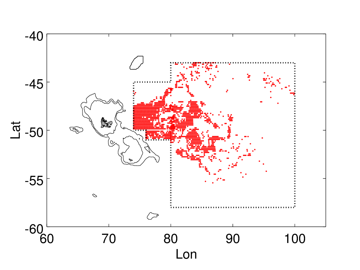
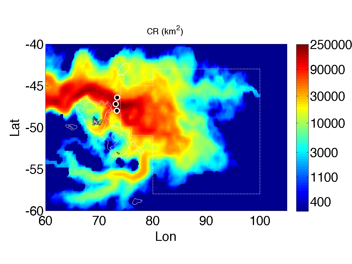
Figure 12: Left panel: Kerguelen plateau with the bloom area delimited by black dotted lines. Bathymetric lines at 500 and 1000 meters. The set of initializing points (shown in red) are selected by choosing the pixels that supported at least one value of chlorophyll greater than $1\,mg/m^{3}$ between November and December 2011 and are showed in red. Each initialization point is assumed to carry an amount of water given by a surface $\Delta=R^{2}\delta_{IG}^{2}$ (when $R$ is the Earth radius and $\delta$ is in radians) for $\delta_{IG}\,=\,0.15\degree$. Right panel: CR computed backward (in log scale), with advection time $\uptau\,=\,180$ days, from the red points showed on the left panel, that cover a total area of about $517000$ km². Black dots represent the first three source stations computed with the CR algorithm described above. Detection range $\sigma\,=\,0.4\degree$

Among them, the Kerguelen plateau is one of the clearest region to show this biogeochemical dynamics and its importance for primary production is now well established. Nevertheless, the hotspots of the continental shelf that may act as main iron sources are still unknown. Here we use the crossroadness computed backward in order to address this question.

Since we want to determine the possible iron sources on the Kerguelen plateau, delimited by the bathymetric line of 1000m, we examine only the region situated eastward to this contour. This is approximated by considering only a region delimited by the perimeter reported in Fig. 12 (left panel, black dotted line). Furthermore, in order to consider only the waters that support a springtime bloom, we analyze satellite-derived images of the chlorophyll patch of spring 2011. We therefore consider as starting points only the pixels that, belonging to the area enclosed by the perimeter, present at least one value of chlorophyll concentration larger than $1\,mg/m^{3}$ during the peak of the bloom of November and December 2011. Note that, in this way, we do not have an initialization grid, but a set of initialization points. The selection is reported on the left panel of Fig. 12 (red points). These points are advected backward for a period of time $\uptau=180$ days, and the crossroadness field is reported in Fig. 12 (right panel). This map highlights a strong passage of water coming from the northern part of the plateau, underlining the central role of the Antarctic Circumpolar Current (ACC) in the advection of waters in proximity of the island platform, and shows also the Southern ACC Front (SACCF) that passes into the Fawn trough. We then use the ranking algorithm in order to locate the most important passage points which feed water to the blooming region. The first three CR stations are all in proximity of the northern part of the plateau, meaning that in the 180 days before the bloom, the largest part (about 70 $\%$) of the water that will sustain primary production, passed through these three points. This analysis locates the Gallieni Spur as a strong candidate where to search for iron sources of the Kerguelen bloom. We note that in general our CR algorithm does not really determine source regions, but rather regions of dense trajectory passage. But since half lifetime of iron in these waters is of the order of about two-three weeks (d’Ovidio et al., 2015), for the value of $\uptau$ used our method in this case should also locate source regions.

4 Discussion and perspectives

Studying dispersion problems, in particular at scales of $\thicksim 10-100\,$kms, (Boyd et al., 2007; Olascoaga et al., 2013; Mahadevan, 2016), is a central issue in many oceanographic problems (Bellingham and Willcox, 1996; Mooers et al., 2005; Bradbury et al., 2008; Rossi et al., 2014; Dubois et al., 2016), whose aim is to achieve good characterization, managing and protective strategies of marine areas and resources. We stress their importance, in particular, for Marine Spatial Planning (MSP). The goal of MSP is indeed to identify the peculiarities, from an ecological or societal point of view (Crowder and Norse, 2008), of the different marine regions, and to map their spatial and temporal distributions in order to manage them in a sustainable way (Ansong et al., 2017; Ehler, 2018). MSP has become, in the last 20 years, a fundamental process in sea management (Douvere, 2008; Muñoz et al., 2015) and is expected to play an increasing important role in the future (e.g., Qiu and Jones, 2013; Magris et al., 2014). An essential component of MSP is the necessity for an effective modeling and monitoring strategy (Ehler, 2017, 2018), a question intimately related to the dispersion of tracers.

In this context, we can identify two main questions.
From one side, we have the case of a passive tracer, advected by the currents. The chaotic and turbulent dynamics characterizing the ocean circulation can disperse the patch and make it spread over a large area (say, of size larger than $100$ km) within a short time (days to weeks). In this case, a recurrent problem is to locate the sites where to deploy observing stations, capable of monitoring or collecting the dispersed tracer (Addison et al., 2018).
A second class of problems concerns the case of a sensible region that is influenced by the circulation upstream (Viikmäe et al., 2011; Delpeche-Ellmann and Soomere, 2013a ; Delpeche-Ellmann and Soomere, 2013b ; Soomere et al., 2015). In this case, the identification of the “sources ”that may affect and spread all over the target area is important for vulnerability assessment (Halpern et al., 2007).
Current methods, mainly based on Lagrangian advection of particles (d’Ovidio et al., 2004; Mancho et al., 2006), concern mostly the identification of coherent regions with minimal transfer of water toward the environs (Haller, 2001; Mancho et al., 2004; Shadden et al., 2005; Beron-Vera et al., 2008). Nevertheless, the knowledge of the spots with enhanced exchanges amongst a flow system is a central issue in dispersion problems (Ser-Giacomi et al., 2015b ; Monroy et al., 2017). The latter question has been recently addressed in the study of Lagrangian Flow Networks (Ser-Giacomi et al., 2015a ; Lindner and Donner, 2017; Rodríguez-Méndez et al., 2017; Fujiwara et al., 2017), in particular with the concept of Most-Probable-Path–betweenness (Ser-Giacomi et al., 2015b ). This diagnostic identifies the choke points in the topology of a flow system. These, nonetheless, are not necessarily spots of major water passage.
Furthermore, to our knowledge, current notions do not solve the problem of displaying and sorting a series of stations in order to answer the two questions mentioned above.
To address these issues, we introduced here a new diagnostic, the crossroadness, which measures the water surface flowing in the neighborhood of a point in a given time window. This has permitted us to develop a ranking method that estimates the places where the majority of the flux passes, and that at the same time sees waters coming from different locations.
This allowed us to design an optimal monitoring system, because each station identified in this way intercepts independent patches of water. We stress that this independence is important for retrieval strategies, for example in the recovering of a contaminant. In fact, in that case the series of the recuperation stations has to be set so that each of them recaptures a different portion of the pollutant that is dispersed. Thus, there is no interest that a station monitors again some waters that have already been intercepted upstream by another one. The same logic is valid in sampling strategies, in which the analysis of the largest surface possible is preferred, and in which sampling twice the same portion of water may be a waste of resources.
Reversing the analysis backward in time we can instead quantify, for each point of the domain, the amount of surface that, passing nearby, will feed a target region. In this case the ranking method identifies the major “source”points from which the water distributes over a vast surface, with each source “irrigating”different areas. The independence of the destinations allows us to maximize the surface covered with a minimal identification of source stations. This is an important factor for the assessment of vulnerable points whose contamination can lead serious damages: for instance, for the protection of Marine Protected Areas (Rengstorf et al., 2013; Ciappa and Costabile, 2014) or hotspots of biological importance (Hobday and Pecl, 2014), like a region with a recurrent bloom that sustains the local trophic chain (Lehahn et al., 2007; Mongin et al., 2008; d’Ovidio et al., 2015). In those cases, it is central to determine the main sites upstream feeding the whole areas.
We first explored the properties of the crossroadness using a steady velocity field obtained from the Navier-Stokes equation (Boffetta et al., 2002; Hairer and Mattingly, 2006), characterized by eddies surrounded by hyperbolic points and manifolds. We showed that the crossroadness is strongly linked to the choice of the initialization grid region. Furthermore, the disposition of the CR stations is not obvious, since they do not necessarily fall on Lagrangian Coherent Structures identified by ridges of Lyapunov exponents, neither their disposition is symmetric, even if the flow stream analyzed is stationary. Interestingly, we found that the stations necessary to monitor all the box cover just the 3% of its surface.
We then applied the previous concepts to the Kerguelen region by considering satellite derived velocity fields. We validated the forward-in-time case by analyzing the trajectories of 43 SVP drifters from KEOPS2 campaign. We showed that 6 stations computed with the crossroadness would have been able to intercept on average about the double of the drifters captured with a regular grid, using the same number of detecting sites. Interestingly, the ratio seemed to improve when diminishing the detection range. We then studied the persistence of an optimal crossroadness network, by looking at how its intercepting capacity degrades when the network is computed from a velocity field previous to the one that disperses the tracer. Even in this case, the crossroadness stations show better performances than regular grids. This is valid also when we consider a region with stronger turbulence. These facts demonstrate how stations computed from past velocity fields can be applied to future circulation patterns, validate furthermore the algorithm proposed and show its robustness when applied to an oceanic environment. It is in fact presumable that, for growing levels of turbulence, the performances of the CR stations, those of a regular grid or a random disposition of the stations would tend to coincide, due to the chaotic activity. However, even when considering a zone with a very strong turbulence (the Kerguelen region), the algorithm showed better performances than a regular grid, meaning that the levels of turbulence activity in ocean do not affect the capacity of the algorithm. The effectiveness of the algorithm does not rely either on a strong detecting power of the stations employed, but on the contrary it improves when diminishing it. The only limitation is the fulfillment of the condition stated in Subsec 2.1, i.e. $\sigma\geq\delta_{IG}$, which could lead potentially to a decrease in the algorithm performance if the detection range considered is smaller than the resolution of the velocity field. We note that our methodology determines inflow and outflow pathways through fixed observation stations. This choice fixes a preferred reference frame. This is at variance with methodologies addressing a different set of problems for which frame-invariance is usually a requirement, such as the computation of Lagrangian coherent structures (Hadjighasem et al., 2017). We use the backward-in-time method to analyse the Kerguelen spring primary production during November-December 2011, showing that about the 70% of the waters that supported the bloom had passed in the vicinity of just 3 sites on the Kerguelen plateau during the previous 6 months, in proximity of the Gallieni Spur.
In our analyses we focused on the properties of the crossroadness considering two-dimensional dynamics. 2D turbulence is in fact present in nature over a large range of scales in which the ratio of lateral and vertical length is very large (Kraichnan and Montgomery, 1980; Tabeling, 2002; Boffetta and Ecke, 2012). When applying these concepts to the oceanic cases, we considered periods of advection sufficiently small in order to neglect vertical velocities. Furthermore, several relevant tracers (in a first approximation) such as plastic, oil and chlorophyl are present almost only in the upper ocean layers, and for their study the 2D approximation can be considered very robust.
We note also that all the analyses provided here can be integrated in a three-dimensional environment, delineating interesting perspectives for future studies.

We note that in a recent paper, Rypina and Pratt, (2017) introduced a “mixing potential”approach which exploits ideas similar to our crossroadness. The main difference is that the mixing potential is a Lagrangian quantity attached to each fluid parcel, whereas our crossroadness uses Lagrangian trajectories but is assigned to each fixed location in space. Thus, whereas the diagnostic in Rypina and Pratt, (2017) may be more appropriate to assess mixing, our approach aims to deploy observation networks and identify sources of transported substances.

There are then several other cases looking interesting for future applications of the crossroadness and its ranking method, and we list here some. For the dispersion of pollutants, the forward in time crossroadness allows us to estimate the most important points in which position a fix station in order to retrieve the contaminant. The aforementioned method can also be used for sampling strategies in order to maximize the surface intercepted and the probability of encountering elements of interest and thus to improve the cost-effectiveness quality (Elliott and Jonge, 1996; Elliott, 2011). In search and rescue operations, if the exact missing point is lacking, and the information available is just on the area of disappearance, computing the forward CR could establish optimal observing stations to look for the lost target. Regarding the backward calculation, this can be used for prioritizing survey locations upstream to vulnerable regions (like Marine Protected Areas), or identifying most likely hotspots close to the shore from which fish larvae may span to a large recruiting area. Our diagnostic provides a direct and simple way to sort a series of stations in order to survey with good performances even very turbulent regions, taking furthermore explicitly into account the detection range.

Appendix A. Temporal persistence of the CR stations along the year

In this Appendix we extend the analysis of Subsec. 3.4 on the possibility of using known velocity fields from the past to obtain sets of CR stations able to monitor transport by future velocity fields.

Drifters intercepted with stations computed along the year.

The SVP drifters release region $\mathcal{R}_{P}$ is advected taking as starting day $D_{0}$ January, 11th, 2011, for a period $\uptau$ of 30 and 60 days, from which 6 CR stations were calculated. They are then used to see how many real drifters from the dataset released on November 2011 they would have intercepted. The computation is repeated changing $D_{0}$, using each time a different month until December, 2011. The results, reported in Fig. A.1, show a better performance of the CR stations compared to the regular grid, along all the year, with a number of drifters intercepted always higher except for one case (August 2011, $\uptau\,=\,60$ days). The case of 60 days advection presents a linear decrease of drifters intercepted for calculations using the three months previous to November, and then a regular increase again, showing a sort of annual cycle, while the 30 days results shows a more irregular trend.

Figure A.1: Number of drifters intercepted using the different months along the year. $\delta_{IG}\,=\,\delta_{OG}\,=\,\sigma=0.2\degree$. Left panel: $\uptau=30\,days$. Right panel: $\uptau=60\,days$ Horizontal lines: values obtained with a regular grid, total (black) and independent (blue line). Note that the release period of the drifters is November 2011.

Figure A.2: Surface of $\mathcal{R}_{P}$, advected from $D_{R}\,=\,$November, 11th, 2011, monitored using the stations computed with velocity currents of different months along the year. $\delta_{IG}\,=\,\delta_{OG}\,=\,0.1\degree$, $\uptau=60\,days$. Left panel: $\sigma\,=\,0.1\degree$. Right panel: $\sigma\,=\,0.2\degree$ Horizontal lines: surface of November monitored using a regular grid (black line) or 6 CR stations (blue line, mean value of the blue circles)

Surface monitored with stations computed along the year.

As in the former case, the region $\mathcal{R}_{P}$ is advected starting from $D_{0}$ January, 11th, 2011, for a period $\uptau$ of 30 and 60 days, and 6 CR stations were computed. This time the stations are not used to see how many SVP drifters they would have collected, but how many trajectories of the set $\mathcal{T}(\mathcal{R})_{D_{R}\rightarrow D_{R}+\uptau}$, with $D_{R}\,=\,$November, 11th, 2011, they would have intercepted. $D_{0}$ is varied taking each time the 11th day of a different month of 2011.

The results are reported in Fig. A.2 and display in both cases a temporal decrease of the surface sampled with the CR stations for the first three months. Generally, the surface monitored with this method is about $15\%$ greater than with a regular grid.

Appendix B. Relation with absolute velocity and mean kinetic energy

A validation of Eqs. (1) and (2) is reported in Fig. B.1, where a map of crossroadness, of kinetic energy and of absolute velocity field, averaged for the month of November, is shown. There, the patterns look pretty identical. This is confirmed by the scatter plot of Fig. B.2, in which the expressions (1) and (2) are represented by the red line. The correlation coefficients of the two plots are very similar, confirming the validation of the assumptions leading to these equations.

Nevertheless, the kinetic energy or speed presents two main differences with the crossroadness, that make them less suitable for monitoring purposes in dispersion problems. In fact, even if these quantities are very similar to CR when the advected area is larger than the domain of calculation, this ceases to be true for smaller advected domains. This is seen in Fig. B.1, lower right panel. There, the crossroadness is computed with the same parameters as in the left upper panel ($\uptau=30$ days, $\delta_{IG}\,=\,\delta_{OG}\,=\,\sigma=0.1\degree$) and on the same observational grid, but the initialization grid is the one used Subsec. 3.2, i.e. much smaller than the observational one. We can notice that the two patterns differ radically, confirming the importance of the fulfillment of the hypothesis leading to Eqs. (1) and (2). Furthermore, simple maps of kinetic energy or speed do not allow to track the origin of the particles that passed through each point, and thus to establish a hierarchy of importance for observing stations.

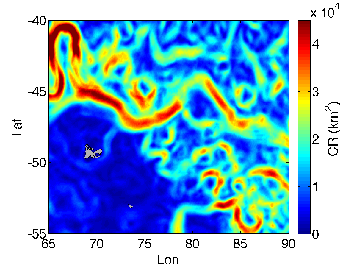
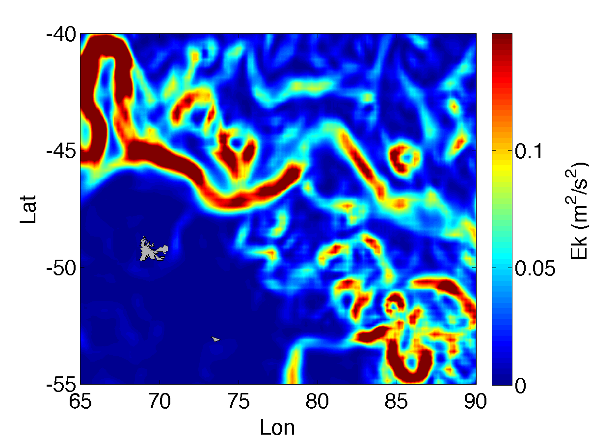
Figure B.1: Top left panel: crossroadness relative to November 2011 computed with an advection time $\uptau=30$ days, $\delta_{IG}\,=\,\delta_{OG}\,=\,\sigma=0.1\degree$. Top right panel: mean kinetic energy $<E_{K}>$ of November 2011. Lower left panel: mean absolute velocity field $<|v|>$ of November 2011. Lower right panel: CR field computed over the same observational grid as in the left upper panel, with same parameters, but the initialization grid is only the drifter release region (rectangle of longitude: [70, 75]$\degree$ and latitude: [-51, -47]$\degree$) as in Subsec. 3.2

Figure B.2: Scatterplot of values of CR vs $<|v|>$ (left panel, correlation coefficient: $0.969$) and CR vs $\sqrt{2<E_{K}>}$ (right panel, correlation coefficient: $0.967$) of Fig. B.1

References

- Abraham and Bowen, (2002) Abraham, E.R., Bowen, M.M., 2002. Chaotic stirring by a mesoscale surface-ocean flow. Chaos: An Interdisciplinary Journal of Nonlinear Science, 12:373–381. doi:https://doi.org/10.1063/1.1481615. PMID: 12779567.
- Addison et al., (2018) Addison, P.F.E., Collins, D.J., Trebilco, R., Howe, S., Bax, N., Hedge, P., Jones, G., Miloslavich, P., Roelfsema, C., Sams, M., Stuart-Smith, R.D., Scanes, P., von Baumgarten, P., McQuatters-Gollop, A., editor: Robert Blasiak, H., 2018. A new wave of marine evidence-based management: emerging challenges and solutions to transform monitoring, evaluating, and reporting. ICES Journal of Marine Science, 75:941–952. doi:10.1093/icesjms/fsx216.
- Andrello et al., (2013) Andrello, M., Mouillot, D., Beuvier, J., Albouy, C., Thuiller, W., Manel, S., 2013. Low connectivity between mediterranean marine protected areas: A biophysical modeling approach for the dusky grouper epinephelus marginatus. PLOS ONE, 8:1–15. doi:10.1371/journal.pone.0068564.
- Ansong et al., (2017) Ansong, J., Gissi, E., Calado, H., 2017. An approach to ecosystem-based management in maritime spatial planning process. Ocean & Coastal Management, 141:65 – 81. doi:https://doi.org/10.1016/j.ocecoaman.2017.03.005.
- Bellingham and Willcox, (1996) Bellingham, J.G., Willcox, J.S., 1996. Optimizing AUV oceanographic surveys. Proceedings of Symposium on Autonomous Underwater Vehicle Technology, pages 391–398. doi:http://dx.doi.org/10.1109/AUV.1996.532439.
- Berline et al., (2014) Berline, L., Rammou, A.M., Doglioli, A., Molcard, A., Petrenko, A., 2014. A connectivity-based eco-regionalization method of the mediterranean sea. PLOS ONE, 9:1–9. doi:10.1371/journal.pone.0111978.
- Beron-Vera et al., (2008) Beron-Vera, F.J., Olascoaga, M.J., Goni, G.J., 2008. Oceanic mesoscale eddies as revealed by lagrangian coherent structures. Geophysical Research Letters, 35. doi:10.1029/2008GL033957.
- Blain et al., (2008) Blain, S., Sarthou, G., Laan, P., 2008. Distribution of dissolved iron during the natural iron-fertilization experiment KEOPS (Kerguelen Plateau, Southern Ocean). Deep Sea Research Part II: Topical Studies in Oceanography, 55:594–605. doi:https://doi.org/10.1016/j.dsr2.2007.12.028.
- Boffetta et al., (2002) Boffetta, G., Celani, A., Musacchio, S., Vergassola, M., 2002. Intermittency in two-dimensional Ekman-Navier-Stokes turbulence. Phys. Rev. E, 66:026304. doi:10.1103/PhysRevE.66.026304.
- Boffetta and Ecke, (2012) Boffetta, G., Ecke, R.E., 2012. Two-Dimensional Turbulence. Annual Review of Fluid Mechanics, 44:427–451. doi:10.1146/annurev-fluid-120710-101240.
- Boffetta et al., (2001) Boffetta, G., Lacorata, G., Redaelli, G., Vulpiani, A., 2001. Detecting barriers to transport: a review of different techniques. Physica D: Nonlinear Phenomena, 159:58–70. doi:http://dx.doi.org/10.1016/S0167-2789(01)00330-X.
- Boffetta and Musacchio, (2010) Boffetta, G., Musacchio, S., 2010. Evidence for the double cascade scenario in two-dimensional turbulence. Phys. Rev. E, 82:016307. doi:10.1103/PhysRevE.82.016307.
- Bouffard et al., (2014) Bouffard, J., Nencioli, F., Escudier, R., Doglioli, A.M., Petrenko, A.A., Pascual, A., Poulain, P.M., Elhmaidi, D., 2014. Lagrangian analysis of satellite-derived currents: Application to the North Western Mediterranean coastal dynamics. Advances in Space Research, 53:788 – 801. doi:https://doi.org/10.1016/j.asr.2013.12.020.
- Boyd et al., (2007) Boyd, P.W., Jickells, T., Law, C.S., Blain, S., Boyle, E.A., Buesseler, K.O., Coale, K.H., Cullen, J.J., de Baar, H.J.W., Follows, M., Harvey, M., Lancelot, C., Levasseur, M., Owens, N.P.J., Pollard, R., Rivkin, R.B., Sarmiento, J., Schoemann, V., Smetacek, V., Takeda, S., Tsuda, A., Turner, S., Watson, A.J., 2007. Mesoscale Iron Enrichment Experiments 1993-2005: Synthesis and Future Directions. Science, 315:612–617. doi:http://dx.doi.org/10.1126/science.1131669.
- Bradbury et al., (2008) Bradbury, I.R., Laurel, B., Snelgrove, P.V., Bentzen, P., Campana, S.E., 2008. Global patterns in marine dispersal estimates: the influence of geography, taxonomic category and life history. Proceedings of the Royal Society of London B: Biological Sciences, 275:1803–1809. doi:http://dx.doi.org/10.1098/rspb.2008.0216.
- Bray et al., (2017) Bray, L., Kassis, D., Hall-Spencer, J., 2017. Assessing larval connectivity for marine spatial planning in the Adriatic. Marine Environmental Research, 125:73 – 81. doi:https://doi.org/10.1016/j.marenvres.2017.01.006.
- Carreras et al., (2017) Carreras, C., Ordóñez, V., Zane, L., Kruschel, C., Nasto, I., Macpherson, E., Pascual, M., 2017. Population genomics of an endemic Mediterranean fish: differentiation by fine scale dispersal and adaptation. Scientific Reports, 7:43417. doi:10.1038/srep43417.
- Christaki et al., (2008) Christaki, U., Obernosterer, I., Van Wambeke, F., Veldhuis, M., Garcia, N., Catala, P., 2008. Microbial food web structure in a naturally iron-fertilized area in the Southern Ocean (Kerguelen Plateau). Deep Sea Research Part II: Topical Studies in Oceanography, 55:706–719. doi:https://doi.org/10.1016/j.dsr2.2007.12.009.
- Ciappa and Costabile, (2014) Ciappa, A., Costabile, S., 2014. Oil spill hazard assessment using a reverse trajectory method for the Egadi marine protected area (Central Mediterranean Sea). Marine Pollution Bulletin, 84:44 – 55. doi:https://doi.org/10.1016/j.marpolbul.2014.05.044.
- Costa et al., (2017) Costa, A., Petrenko, A.A., Guizien, K., Doglioli, A.M., 2017. On the calculation of betweenness centrality in marine connectivity studies using transfer probabilities. PLOS ONE, 12:1–10. doi:10.1371/journal.pone.0189021.
- Cowen et al., (2006) Cowen, R.K., Paris, C.B., Srinivasan, A., 2006. Scaling of Connectivity in Marine Populations. Science, 311:522–527. doi:10.1126/science.1122039.
- Crowder and Norse, (2008) Crowder, L., Norse, E., 2008. Essential ecological insights for marine ecosystem-based management and marine spatial planning. Marine Policy, 32:772 – 778. doi:https://doi.org/10.1016/j.marpol.2008.03.012. The Role of Marine Spatial Planning in Implementing Ecosystem-based, Sea Use Management.
- de Jonge et al., (2006) de Jonge, V., Elliott, M., Brauer, V., 2006. Marine monitoring: Its shortcomings and mismatch with the EU Water Framework Directive’s objectives. Marine Pollution Bulletin, 53:5 – 19. doi:https://doi.org/10.1016/j.marpolbul.2005.11.026. Recent Developments in Estuarine Ecology and Management.
- (24) Delpeche-Ellmann, N.C., Soomere, T., 2013a. Investigating the Marine Protected Areas most at risk of current-driven pollution in the Gulf of Finland, the Baltic Sea, using a Lagrangian transport model. Marine Pollution Bulletin, 67:121 – 129. doi:https://doi.org/10.1016/j.marpolbul.2012.11.025.
- (25) Delpeche-Ellmann, N.C., Soomere, T., 2013b. Using Lagrangian models to assist in maritime management of Coastal and Marine Protected Areas. Journal of Coastal Research, pages 36–41. doi:10.2112/SI65-007.1.
- Douvere, (2008) Douvere, F., 2008. The importance of marine spatial planning in advancing ecosystem-based sea use management. Marine Policy, 32:762 – 771. doi:https://doi.org/10.1016/j.marpol.2008.03.021. The Role of Marine Spatial Planning in Implementing Ecosystem-based, Sea Use Management.
- d’Ovidio et al., (2013) d’Ovidio, F., De Monte, S., Della Penna, A., Cotté, C., Guinet, C., 2013. Ecological implications of eddy retention in the open ocean: a Lagrangian approach. Journal of Physics A: Mathematical and Theoretical, 46:254023. doi:10.1088/1751-8113/46/25/254023.
- d’Ovidio et al., (2015) d’Ovidio, F., Della Penna, A., Trull, T.W., Nencioli, F., Pujol, M.I., Rio, M.H., Park, Y.H., Cotté, C., Zhou, M., Blain, S., 2015. The biogeochemical structuring role of horizontal stirring: Lagrangian perspectives on iron delivery downstream of the Kerguelen plateau. Biogeosciences, 12:5567–5581. doi:https://doi.org/10.5194/bg-12-5567-2015.
- d’Ovidio et al., (2004) d’Ovidio, F., Fernández, V., Hernández-García, E., López, C., 2004. Mixing structures in the Mediterranean Sea from finite-size Lyapunov exponents. Geophysical Research Letters, 31. doi:http://dx.doi.org/10.1029/2004GL020328.
- Dubois et al., (2016) Dubois, M., Rossi, V., Ser-Giacomi, E., Arnaud-Haond, S., López, C., Hernández-García, E., 2016. Linking basin-scale connectivity, oceanography and population dynamics for the conservation and management of marine ecosystems. Global Ecology and Biogeography, 25:503–515. doi:https://doi.org/10.1111/geb.12431.
- Eckart, (1948) Eckart, C., 1948. An analysis of the stirring and mixing processes in incompressible fluids. Journal of Marine Research, 7:265–275.
- Ehler, (2017) Ehler, C., 2017. A Guide to Evaluating Marine Spatial Plans. doi:10.17605/OSF.IO/HY9RS.
- Ehler, (2018) Ehler, C.N.N., 2018. Marine spatial planning. Offshore Energy and Marine Spatial Planning, pages 6–17.
- Elliott, (2011) Elliott, M., 2011. Marine science and management means tackling exogenic unmanaged pressures and endogenic managed pressures – A numbered guide. Marine Pollution Bulletin, 62:651 – 655. doi:https://doi.org/10.1016/j.marpolbul.2010.11.033.
- Elliott and Jonge, (1996) Elliott, M., Jonge, V.N.D., 1996. The need for monitoring the monitors and their monitoring. Marine Pollution Bulletin, 32:248 – 249. doi:https://doi.org/10.1016/0025-326X(96)00009-4.
- Froyland et al., (2007) Froyland, G., Padberg, K., England, M.H., Treguier, A.M., 2007. Detection of Coherent Oceanic Structures via Transfer Operators. Phys. Rev. Lett., 98:224503. doi:10.1103/PhysRevLett.98.224503.
- Froyland et al., (2014) Froyland, G., Stuart, R.M., van Sebille, E., 2014. How well-connected is the surface of the global ocean? Chaos: An Interdisciplinary Journal of Nonlinear Science, 24:033126. doi:10.1063/1.4892530.
- Fujiwara et al., (2017) Fujiwara, N., Kirchen, K., Donges, J.F., Donner, R.V., 2017. A perturbation-theoretic approach to Lagrangian flow networks. Chaos, 27:035813. doi:10.1063/1.4978549.
- Garrett, (1983) Garrett, C., 1983. On the initial streakness of a dispersing tracer in two-and three-dimensional turbulence. Dynamics of Atmospheres and Oceans, 7:265–277. doi:https://doi.org/10.1016/0377-0265(83)90008-8.
- Gopalakrishnan Meena et al., (2018) Gopalakrishnan Meena, M., Nair, A.G., Taira, K., 2018. Network community-based model reduction for vortical flows. Phys. Rev. E, 97:063103. doi:10.1103/PhysRevE.97.063103.
- Hadjighasem et al., (2017) Hadjighasem, A., Farazmand, M., Blazevski, D., Froyland, G., Haller, G., 2017. A critical comparison of lagrangian methods for coherent structure detection. Chaos: An Interdisciplinary Journal of Nonlinear Science, 27:053104. doi:10.1063/1.4982720.
- Hadjighasem et al., (2016) Hadjighasem, A., Karrasch, D., Teramoto, H., Haller, G., 2016. Spectral-clustering approach to Lagrangian vortex detection. Physical Review E, 93:063107. doi:10.1103/PhysRevE.93.063107.
- Hairer and Mattingly, (2006) Hairer, M., Mattingly, J.C., 2006. Ergodicity of the 2D Navier-Stokes Equations with Degenerate Stochastic Forcing. Annals of Mathematics, 164:993–1032.
- Haller, (2001) Haller, G., 2001. Lagrangian structures and the rate of strain in a partition of two-dimensional turbulence. Physics of Fluids, 13:3365–3385. doi:doi:10.1063/1.1403336.
- Haller and Yuan, (2000) Haller, G., Yuan, G., 2000. Lagrangian coherent structures and mixing in two-dimensional turbulence. Phys. D, 147:352–370. doi:10.1016/S0167-2789(00)00142-1.
- Halpern et al., (2007) Halpern, B.S., Selkoe, K.A., Micheli, F., Kappel, C.V., 2007. Evaluating and Ranking the Vulnerability of Global Marine Ecosystems to Anthropogenic Threats. Conservation Biology, 21:1301–1315. doi:10.1111/j.1523-1739.2007.00752.x.
- Hobday and Pecl, (2014) Hobday, A.J., Pecl, G.T., 2014. Identification of global marine hotspots: sentinels for change and vanguards for adaptation action. Reviews in Fish Biology and Fisheries, 24:415–425. doi:10.1007/s11160-013-9326-6.
- Iacobello et al., (2018) Iacobello, G., Scarsoglio, S., Ridolfi, L., 2018. Visibility graph analysis of wall turbulence time-series. Physics Letters A, 382:1 – 11. doi:https://doi.org/10.1016/j.physleta.2017.10.027.
- Koltai and Renger, (2018) Koltai, P., Renger, D.R.M., 2018. From Large Deviations to Semidistances of Transport and Mixing: Coherence Analysis for Finite Lagrangian Data. Journal of Nonlinear Science. doi:10.1007/s00332-018-9471-0.
- Kraichnan and Montgomery, (1980) Kraichnan, R.H., Montgomery, D., 1980. Two-dimensional turbulence. Reports on Progress in Physics, 43:547.
- Lam and Bishop, (2008) Lam, P.J., Bishop, J.K., 2008. The continental margin is a key source of iron to the HNLC North Pacific Ocean. Geophysical Research Letters, 35. doi:http://dx.doi.org/10.1029/2008GL033294.
- Lehahn et al., (2007) Lehahn, Y., d’Ovidio, F., Lévy, M., Heifetz, E., 2007. Stirring of the northeast Atlantic spring bloom: A Lagrangian analysis based on multisatellite data. Journal of Geophysical Research, 112:C08005. doi:http://dx.doi.org/10.1029/2006JC003927.
- Lindner and Donner, (2017) Lindner, M., Donner, R.V., 2017. Spatio-temporal organization of dynamics in a two-dimensional periodically driven vortex flow: A Lagrangian flow network perspective. Chaos: An Interdisciplinary Journal of Nonlinear Science, 27:035806. doi:https://doi.org/10.1063/1.4975126.
- Magris et al., (2014) Magris, R.A., Pressey, R.L., Weeks, R., Ban, N.C., 2014. Integrating connectivity and climate change into marine conservation planning. Biological Conservation, 170:207 – 221. doi:https://doi.org/10.1016/j.biocon.2013.12.032.
- Mahadevan, (2016) Mahadevan, A., 2016. The impact of submesoscale physics on primary productivity of plankton. Annual review of marine science, 8:161–184.
- Mancho et al., (2004) Mancho, A., Small, D., Wiggins, S., 2004. Computation of hyperbolic trajectories and their stable and unstable manifolds for oceanographic flows represented as data sets. Nonlinear Processes in Geophysics, 11:17–33.
- Mancho et al., (2006) Mancho, A.M., Small, D., Wiggins, S., 2006. A tutorial on dynamical systems concepts applied to lagrangian transport in oceanic flows defined as finite time data sets: Theoretical and computational issues. Physics Reports, 437:55–124. doi:10.1016/j.physrep.2006.09.005.
- Martin et al., (2013) Martin, P., Loeff, M.R., Cassar, N., Vandromme, P., d’Ovidio, F., Stemmann, L., Rengarajan, R., Soares, M., González, H.E., Ebersbach, F., Lampitt, R.S., Sanders, R., Barnett, B.A., Smetacek, V., Naqvi, S.W.A., 2013. Iron fertilization enhanced net community production but not downward particle flux during the Southern Ocean iron fertilization experiment LOHAFEX. Global Biogeochemical Cycles, 27:871–881. doi:http://dx.doi.org/10.1002/gbc.20077.
- McAdam and van Sebille, (2018) McAdam, R., van Sebille, E., 2018. Surface Connectivity and Inter-ocean Exchanges From Drifter-Based Transition Matrices. Journal of Geophysical Research: Oceans, pages n/a–n/a. doi:10.1002/2017JC013363.
- Melià et al., (2016) Melià, P., Schiavina, M., Rossetto, M., Gatto, M., Fraschetti, S., Casagrandi, R., 2016. Looking for hotspots of marine metacommunity connectivity: a methodological framework. Scientific Reports, 6:23705.
- Miron et al., (2017) Miron, P., Beron-Vera, F.J., Olascoaga, M.J., Sheinbaum, J., Pérez-Brunius, P., Froyland, G., 2017. Lagrangian dynamical geography of the Gulf of Mexico. Scientific reports, 7:7021.
- Molkenthin et al., (2017) Molkenthin, N., Kutza, H., Tupikina, L., Marwan, N., Donges, J.F., Feudel, U., Kurths, J., Donner, R.V., 2017. Edge anisotropy and the geometric perspective on flow networks. Chaos: An Interdisciplinary Journal of Nonlinear Science, 27:035802. doi:10.1063/1.4971785.
- Mongin et al., (2008) Mongin, M., Molina, E., Trull, T.W., 2008. Seasonality and scale of the kerguelen plateau phytoplankton bloom: A remote sensing and modeling analysis of the influence of natural iron fertilization in the southern ocean. Deep Sea Research Part II: Topical Studies in Oceanography, 55:880 – 892. doi:https://doi.org/10.1016/j.dsr2.2007.12.039. KEOPS: Kerguelen Ocean and Plateau compared Study.
- Monroy et al., (2017) Monroy, P., Rossi, V., Ser-Giacomi, E., López, C., Hernández-García, E., 2017. Sensitivity and robustness of larval connectivity diagnostics obtained from Lagrangian Flow Networks. ICES Journal of Marine Science, 74:1763–1779. doi:http://dx.doi.org/10.1093/icesjms/fsw235.
- Mooers et al., (2005) Mooers, C., Meinen, C., Baringer, M., Bang, I., Rhodes, R., Barron, C.N., Bub, F., 2005. Cross validating ocean prediction and monitoring systems. Eos, Transactions American Geophysical Union, 86:269–273. doi:http://dx.doi.org/10.1029/2005EO290002.
- Muñoz et al., (2015) Muñoz, M., Reul, A., Plaza, F., Gómez-Moreno, M.L., Vargas-Yañez, M., Rodríguez, V., Rodríguez, J., 2015. Implication of regionalization and connectivity analysis for marine spatial planning and coastal management in the Gulf of Cadiz and Alboran Sea. Ocean & Coastal Management, 118:60 – 74. doi:https://doi.org/10.1016/j.ocecoaman.2015.04.011. Coastal systems under change.
- Nencioli et al., (2011) Nencioli, F., d’Ovidio, F., Doglioli, A., Petrenko, A., 2011. Surface coastal circulation patterns by in situ detection of Lagrangian coherent structures. Geophysical Research Letters, 38. doi:10.1029/2011GL048815.
- Okubo, (1978) Okubo, A., 1978. Horizontal Dispersion and Critical Scales for Phytoplankton Patches. Spatial pattern in plankton communities, 3:21–42. doi:10.1007/978-1-4899-2195-6˙2.
- Olascoaga et al., (2013) Olascoaga, M.J., Beron-Vera, F.J., Haller, G., Trinanes, J., Iskandarani, M., Coelho, E., Haus, B.K., Huntley, H., Jacobs, G., Kirwan, A., et al., 2013. Drifter motion in the gulf of mexico constrained by altimetric lagrangian coherent structures. Geophysical Research Letters, 40:6171–6175.
- Ottino, (1989) Ottino, J.M., 1989. The kinematics of mixing: stretching, chaos, and transport, volume 3 of Cambridge Texts in Applied Mathematics. Cambridge University Press.
- Padberg-Gehle and Schneide, (2017) Padberg-Gehle, K., Schneide, C., 2017. Network-based study of Lagrangian transport and mixing. Nonlinear Processes in Geophysics, 24:661–671.
- Park et al., (2014) Park, Y.H., Durand, I., Kestenare, E., Rougier, G., Zhou, M., d’Ovidio, F., Cotté, C., Lee, J.H., 2014. Polar Front around the Kerguelen Islands: An up-to-date determination and associated circulation of surface/subsurface waters. Journal of Geophysical Research: Oceans, 119:6575–6592. doi:http://dx.doi.org/10.1002/2014JC010061.
- Phillips et al., (2015) Phillips, J.D., Schwanghart, W., Heckmann, T., 2015. Graph theory in the geosciences. Earth-Science Reviews, 143:147 – 160. doi:https://doi.org/10.1016/j.earscirev.2015.02.002.
- Planes et al., (2009) Planes, S., Jones, G.P., Thorrold, S.R., 2009. Larval dispersal connects fish populations in a network of marine protected areas. Proceedings of the National Academy of Sciences, 106:5693–5697. doi:http://dx.doi.org/10.1073/pnas.0808007106.
- (75) Prants, S., Budyansky, M., Uleysky, M.Y., 2014a. Identifying Lagrangian fronts with favourable fishery conditions. Deep Sea Research Part I: Oceanographic Research Papers, 90:27–35. doi:https://doi.org/10.1016/j.dsr.2014.04.012.
- (76) Prants, S., Budyansky, M., Uleysky, M.Y., 2014b. Lagrangian fronts in the ocean. Izvestiya, Atmospheric and Oceanic Physics, 50:284–291. doi:https://doi.org/10.1134/S0001433814030116.
- Pujol et al., (2016) Pujol, M.I., Faugère, Y., Taburet, G., Dupuy, S., Pelloquin, C., Ablain, M., Picot, N., 2016. DUACS DT2014: the new multi-mission altimeter data set reprocessed over 20 years. Ocean Science, 12:1067–1090. doi:https://doi.org/10.5194/os-12-1067-2016.
- Qiu and Jones, (2013) Qiu, W., Jones, P.J., 2013. The emerging policy landscape for marine spatial planning in Europe. Marine Policy, 39:182 – 190. doi:https://doi.org/10.1016/j.marpol.2012.10.010.
- Rengstorf et al., (2013) Rengstorf, A.M., Yesson, C., Brown, C., Grehan, A.J., 2013. High-resolution habitat suitability modelling can improve conservation of vulnerable marine ecosystems in the deep sea. Journal of Biogeography, 40:1702–1714. doi:10.1111/jbi.12123.
- Rodríguez-Méndez et al., (2017) Rodríguez-Méndez, V., Ser-Giacomi, E., Hernández-García, E., 2017. Clustering coefficient and periodic orbits in flow networks. Chaos: An Interdisciplinary Journal of Nonlinear Science, 27:035803. doi:https://doi.org/10.1063/1.4971787.
- Rossi et al., (2014) Rossi, V., Ser-Giacomi, E., López, C., Hernández-García, E., 2014. Hydrodynamic provinces and oceanic connectivity from a transport network help designing marine reserves. Geophysical Research Letters, 41:2883–2891.
- Rypina and Pratt, (2017) Rypina, I.I., Pratt, L.J., 2017. Trajectory encounter volume as a diagnostic of mixing potential in fluid flows. Nonlinear Processes in Geophysics, 24:189. doi:https://doi.org/10.5194/npg-24-189-2017.
- Ser-Giacomi et al., (2017) Ser-Giacomi, E., Rodríguez-Méndez, V., López, C., Hernández-García, E., 2017. Lagrangian Flow Network approach to an open flow model. The European Physical Journal Special Topics, 226:2057–2068. doi:https://doi.org/10.1140/epjst/e2017-70044-2.
- (84) Ser-Giacomi, E., Rossi, V., López, C., Hernández-García, E., 2015a. Flow networks: A characterization of geophysical fluid transport. Chaos: An Interdisciplinary Journal of Nonlinear Science, 25:036404. doi:https://doi.org/10.1063/1.4908231.
- (85) Ser-Giacomi, E., Vasile, R., Hernández-García, E., López, C., 2015b. Most probable paths in temporal weighted networks: An application to ocean transport. Physical Review E, 92:012818. doi:10.1103/PhysRevE.92.012818.
- (86) Ser-Giacomi, E., Vasile, R., Recuerda, I., Hernández-García, E., López, C., 2015c. Dominant transport pathways in an atmospheric blocking event. Chaos: An Interdisciplinary Journal of Nonlinear Science, 25:087413. doi:10.1063/1.4928704.
- Shadden et al., (2005) Shadden, S.C., Lekien, F., Marsden, J.E., 2005. Definition and properties of lagrangian coherent structures from finite-time lyapunov exponents in two-dimensional aperiodic flows. Physica D: Nonlinear Phenomena, 212:271–304. doi:10.1016/j.physd.2005.10.007.
- Shanks, (2009) Shanks, A.L., 2009. Pelagic Larval Duration and Dispersal Distance Revisited. The Biological Bulletin, 216:373–385. doi:10.1086/BBLv216n3p373. PMID: 19556601.
- Siegel et al., (2008) Siegel, D.A., Mitarai, S., Costello, C.J., Gaines, S.D., Kendall, B.E., Warner, R.R., Winters, K.B., 2008. The stochastic nature of larval connectivity among nearshore marine populations. Proceedings of the National Academy of Sciences. doi:10.1073/pnas.0802544105.
- Soomere et al., (2015) Soomere, T., Delpeche-Ellmann, N., Torsvik, T., Viikmäe, B., 2015. Towards a New Generation of Techniques for the Environmental Management of Maritime Activities. In Environmental Security of the European Cross-Border Energy Supply Infrastructure, pages 103–132. Springer. doi:10.1007/978-94-017-9538-8˙8.
- Sundermeyer and Price, (1998) Sundermeyer, M.A., Price, J.F., 1998. Lateral mixing and the North Atlantic Tracer Release Experiment: Observations and numerical simulations of Lagrangian particles and a passive tracer. Journal of Geophysical Research: Oceans, 103:21481–21497. doi:http://dx.doi.org/10.1029/98JC01999.
- Suneel et al., (2016) Suneel, V., Ciappa, A., Vethamony, P., 2016. Backtrack modeling to locate the origin of tar balls depositing along the west coast of India. Science of The Total Environment, 569-570:31 – 39. doi:https://doi.org/10.1016/j.scitotenv.2016.06.101.
- Tabeling, (2002) Tabeling, P., 2002. Two-dimensional turbulence: a physicist approach. Physics Reports, 362:1 – 62. doi:https://doi.org/10.1016/S0370-1573(01)00064-3.
- Viikmäe et al., (2011) Viikmäe, B., Soomere, T., Parnell, K., Delpeche, N., 2011. Spatial planning of shipping and offshore activities in the Baltic Sea using Lagrangian trajectories. Journal of Coastal Research, page 956.
- Vrana et al., (2005) Vrana, B., Allan, I.J., Greenwood, R., Mills, G.A., Dominiak, E., Svensson, K., Knutsson, J., Morrison, G., 2005. Passive sampling techniques for monitoring pollutants in water. TrAC Trends in Analytical Chemistry, 24:845–868. doi:https://doi.org/10.1016/j.trac.2005.06.006.
- Wiggins, (2005) Wiggins, S., 2005. The dynamical systems approach to Lagrangian transport in oceanic flows. Annual Review of Fluid Mechanics, 37:295–328. doi:https://doi.org/10.1146/annurev.fluid.37.061903.175815.