Topologically Controlled Lossy Compression

Abstract

This paper presents a new algorithm for the lossy compression of scalar data defined on 2D or 3D regular grids, with topological control. Certain techniques allow users to control the pointwise error induced by the compression. However, in many scenarios it is desirable to control in a similar way the preservation of higher-level notions, such as topological features , in order to provide guarantees on the outcome of post-hoc data analyses. This paper presents the first compression technique for scalar data which supports a strictly controlled loss of topological features. It provides users with specific guarantees both on the preservation of the important features and on the size of the smaller features destroyed during compression. In particular, we present a simple compression strategy based on a topologically adaptive quantization of the range. Our algorithm provides strong guarantees on the bottleneck distance between persistence diagrams of the input and decompressed data, specifically those associated with extrema. A simple extension of our strategy additionally enables a control on the pointwise error. We also show how to combine our approach with state-of-the-art compressors, to further improve the geometrical reconstruction. Extensive experiments, for comparable compression rates, demonstrate the superiority of our algorithm in terms of the preservation of topological features. We show the utility of our approach by illustrating the compatibility between the output of post-hoc topological data analysis pipelines, executed on the input and decompressed data, for simulated or acquired data sets. We also provide a lightweight VTK-based C++ implementation of our approach for reproduction purposes.

Introduction

Data compression is an important tool for the analysis and visualization of large data sets. In particular, in the context of high performance computing, current trends and predictions [39] indicate increases of the number of cores in super-computers which evolve faster than their memory, IO and network bandwidth. This observation implies that such machines tend to compute results faster than they are able to store or transfer them. Thus, data movement is now recognized as an important bottleneck which challenges large-scale scientific simulations. This challenges even further post-hoc data exploration and interactive analysis, as the output data of simulations often needs to be transferred to a commodity workstation to conduct such interactive inspections. Not only such a transfer is costly in terms of time, but data can often be too large to fit in the memory of a workstation. In this context, data reduction and compression techniques are needed to reduce the amount of data to transfer.

While many lossless compression techniques are now well established [25, 47, 48, 33], scientific data sets often need to be compressed at more aggressive rates, which requires lossy techniques [28, 31] (i.e. compression which alters the data). In the context of post-hoc analysis and visualization of data which has been compressed with a lossy technique, it is important for users to understand to what extent their data has been altered, to make sure that such an alteration has no impact on the analysis. This motivates the design of lossy compression techniques with error guarantees.

Several lossy techniques with guarantees have been documented, with a particular focus on pointwise error [33, 27, 12]. However, pointwise error is a low level measure and it can be difficult for users to apprehend its propagation through their analysis pipeline, and consequently its impact on the outcome of their analysis. Therefore, it may be desirable to design lossy techniques with guarantees on the preservation of higher-level notions, such as the features of interest in the data. However, the definition of features primarily depends on the target application, but also on the type of analysis pipeline under consideration. This motivates, for each possible feature definition, the design of a corresponding lossy compression strategy with guarantees on the preservation of the said features. In this work, we introduce a lossy compression technique that guarantees the preservation of features of interest, defined with topological notions, hence providing users with strong guarantees when post-analyzing their data with topological methods.

Topological data analysis techniques [13, 35, 23] have demonstrated their ability over the last two decades to capture in a generic, robust and efficient manner features of interest in scalar data, for many applications: turbulent combustion [5], computational fluid dynamics [16], chemistry [18], astrophysics [40], etc. One reason for the success of topological methods in applications is the possibility for domain experts to easily translate high level notions into topological terms. For instance, the cosmic web in astrophysics can be extracted by querying the most persistent one-dimensional separatrices of the Morse-Smale complex connected to maxima of matter density [40]. Many similar feature definitions in topological terms can be found in the above application examples. For instance, we detail in subsection 4.3 two analysis pipelines based on topological methods for the segmentation of acquired and simulated data. In the first case, features of interest (bones in a medical CT scan) can be extracted as the regions of space corresponding to the arcs of the split tree [8] which are attached to local maxima of CT intensity. In this scenario, it is important that lossy compression alters the data in a way that guarantees to preserve the split tree, to guarantee a faithful segmentation despite compression and thus, to enable further measurement, analysis and diagnosis even after compression. Thus, it is necessary, for all applications involving topological methods in their post-hoc analysis, to design lossy compression techniques with topological guarantees.

This paper presents, to the best of our knowledge, the first lossy compression technique for scalar data with such topological guarantees. In particular, we introduce a simple algorithm based on a topologically adaptive quantization of the data range. We carefully study the stability of the persistence diagram [14, 11] of the decompressed data compared to the original one. Given a target feature size to preserve, which is expressed as a persistence threshold $\epsilon$, our algorithm exactly preserves the critical point pairs with persistence greater than $\epsilon$ and destroys all pairs with smaller persistence. We provide guarantees on the bottleneck and Wasserstein distances between the persistence diagrams, expressed as a function of the input parameter $\epsilon$. Simple extensions to our strategy additionally enable to include a control on the pointwise error and to combine our algorithm with state-of-the-art compressors to improve the geometry of the reconstruction, while still providing strong topological guarantees. Extensive experiments, for comparable compression rates, demonstrate the superiority of our technique for the preservation of topological features. We show the utility of our approach by illustrating the compatibility between the output of topological analysis pipelines, executed on the original and decompressed data, for simulated or acquired data (subsection 4.3). We also provide a VTK-based C++ implementation of our approach for reproduction purposes.

0.1 Related work

Related existing techniques can be classified into two main categories, addressing lossless and lossy compression respectively.

Regarding lossless compression, several general purpose algorithms have been documented, using entropy encoders [24, 17, 6, 25], dictionaries [47, 48] and predictors [7, 10]. For instance, the compressors associated with the popular file format Zip rely on a combination of the LZ77 algorithm [47] and Huffman coding [25]. Such compressors replace recurrent bit patterns in the data by references to a single copy of the pattern. Thus, these approaches reach particularly high compression rates when a high redundancy is present in the data. Several statistical [26, 33] or non-statistical [36] approaches have been proposed for volume data but often achieve insufficient compression rates in applications (below two [31]), hence motivating lossy compression techniques.

Regarding lossy compression, many strategies have been documented. Some of them are now well established and implemented in international standards, such as GIF or JPEG. Such approaches rely for instance on vector quantization [37] or discrete cosine [29] and related block transforms [31]. However, relatively little work, mostly related to scientific computing applications, has yet focused on the definition of lossy compression techniques with an emphasis on error control, mostly expressed as a bound on the pointwise error. For instance, though initially introduced for lossless compression, the FPZIP compressor [33] supports truncation of floating point values, thus providing an explicit relative error control. The Isabela compressor [28] supports predictive temporal compression by B-spline fitting and analysis of quantized error. The fixed rate compressor ZFP [31], based on local block transforms, supports maximum error control by not ignoring transform coefficients whose effect on the output is more than a user defined error threshold [32]. More recently, Di and Cappello [12] introduced a compressor based on curve fitting specifically designed for pointwise error control. This control is enforced by explicitly storing values for which the curve fitting exceeds the input error tolerance. Iverson et al. [27] also introduced a compressor, named SQ, specifically designed for absolute error control. It supports a variety of strategies based on range quantization and/or region growing with an error-based stopping condition. For instance, given an input error tolerance $\epsilon$, the quantization approach segments the range in contiguous intervals of width $\epsilon$. Then, the scalar value of each grid vertex is encoded by the identifier of the interval it projects to in the range. At decompression, all vertices sharing a unique interval identifier are given a common scalar value (the middle of the corresponding interval), effectively guaranteeing a maximum error of $\epsilon$ (for vertices located in the vicinity of an interval bound). Such a range quantization strategy is particularly appealing for the preservation of topological features, as one of the key stability results on persistence diagrams [14] states that the bottleneck distance between the diagrams of two scalar functions is bounded by their maximum pointwise error [11]. Intuitively, this means that all critical point pairs with persistence higher than $\epsilon$ in the input will still be present after a compression based on range quantization. However, a major drawback of such a strategy is the constant quantization step size, which implies that large parts of the range, possibly devoid of important topological features, will still be decomposed into contiguous intervals of width $\epsilon$, hence drastically limiting the compression rate in practice. In contrast, our approach is based on a topologically adaptive range quantization which precisely addresses this drawback, enabling superior compression rates. We additionally show how to extend our approach with absolute pointwise error control. As detailed in Sec. 2.3, this strategy preserves persistence pairs with persistence larger than $\epsilon$, exactly. In contrast, since it snaps values to the middle of intervals, simple range quantization [27] may alter the persistence of critical point pairs in the decompressed data, by increasing the persistence of smaller pairs (noise) and/or decreasing that of larger pairs (features). Such an alteration is particularly concerning for post-hoc analyses, as it degrades the separation of noise from features and prevents a reliable post-hoc multi-scale analysis, as the preservation of the persistence of critical point pairs is no longer guaranteed. Finally, note that a few approaches also considered topological aspects [2, 3, 41] but for the compression of meshes, not of scalar data.

0.2 Contributions

This paper makes the following new contributions:

1. Approach: We present the first algorithm for data compression specifically designed to enforce topological control. We present a simple strategy and carefully describe the stability of the persistence diagram of the output data. In particular, we show that, given a target feature size (i.e. persistence) to preserve, our approach minimizes both the bottleneck and Wasserstein distances between the persistence diagrams of the input and decompressed data.

2. Extensions: We show how this strategy can be easily extended to additionally include control on the maximum pointwise error. Further, we show how to combine our compressor with state-of-the-art compressors, to improve the average error.

3. Application: We present applications of our approach to post-hoc analyses of simulated and acquired data, where users can faithfully conduct advanced topological data analysis on compressed data, with guarantees on the maximal size of missing features and the exact preservation of the most important ones.

4. Implementation: We provide a lightweight VTK-based C++ implementation of our approach for reproduction purposes.

1 Preliminaries

This section briefly describes our formal setting and presents an overview of our approach. An introduction to topological data analysis can be found in [13].

1.1 Background

Input data: Without loss of generality, we assume that the input data is a piecewise linear (PL) scalar field $f:\mathcal{M}\rightarrow\mathbb{R}$ defined on a PL $d$-manifold $\mathcal{M}$ with $d$ equals 2 or 3. It has value at the vertices of $\mathcal{M}$ and is linearly interpolated on the simplices of higher dimension. Adjacency relations on $\mathcal{M}$ can be described in a dimension independent way. The star $St(v)$ of a vertex $v$ is the set of simplices of $\mathcal{M}$ which contain $v$ as a face. The link $Lk(v)$ is the set of faces of the simplices of $St(v)$ which do not intersect $v$. The topology of $\mathcal{M}$ can be described with its Betti numbers $\beta_{i}$ (the ranks of its homology groups [13]), which correspond in 3D to the numbers of connected components ($\beta_{0}$), non collapsible cycles ($\beta_{1}$) and voids ($\beta_{2}$).

Critical points: For visualization and data analysis purposes, several low-level geometric features can be defined given the input data. Given an isovalue $i\in\mathbb{R}$, the sub-level set of $i$, noted $f^{-1}_{-\infty}(i)$, is defined as the pre-image of the open interval $(-\infty,i)$ onto $\mathcal{M}$ through $f$: $f^{-1}_{-\infty}(i)=\{p\in\mathcal{M}~{}|~{}f(p)<i\}$. Symmetrically, the sur-level set $f^{-1}_{+\infty}(i)$ is defined by $f^{-1}_{+\infty}(i)=\{p\in\mathcal{M}~{}|~{}f(p)>i\}$. These two objects serve as fundamental segmentation tools in many analysis tasks [5]. The points of $\mathcal{M}$ where the Betti numbers of $f^{-1}_{-\infty}(i)$ change are the critical points of $f$ (Fig. 1) and their associated $f$ values are called critical values. Let $Lk^{-}(v)$ be the lower link of the vertex $v$: $Lk^{-}(v)=\{\sigma\in Lk(v)~{}|~{}\forall u\in\sigma:f(u)<f(v)\}$. The upper link $Lk^{+}(v)$ is given by $Lk^{+}(v)=\{\sigma\in Lk(v)~{}|~{}\forall u\in\sigma:f(u)>f(v)\}$. To classify $Lk(v)$ without ambiguity into either lower or upper links, the restriction of $f$ to the vertices of $\mathcal{M}$ is assumed to be injective. This is easily enforced in practice by a variant of simulation of simplicity [15]. This is achieved by considering an associated injective integer offset $\mathcal{O}_{f}(v)$, which initially typically corresponds to the vertex position offset in memory. Then, when comparing two vertices, if these share the same value $f$, their order is disambiguated by their offset $\mathcal{O}_{f}$. A vertex $v$ is regular, if and only if both $Lk^{-}(v)$ and $Lk^{+}(v)$ are simply connected. Otherwise, $v$ is a critical point of $f$. Let $d$ be the dimension of $\mathcal{M}$. Critical points can be classified with their index $\mathcal{I}$, which equals 0 for minima ($Lk^{-}(v)=\emptyset$), 1 for 1-saddles ($\beta_{0}(Lk^{-}(v))=2$), $(d-1)$ for $(d-1)$-saddles ($\beta_{0}(Lk^{+}(v))=2$) and $d$ for maxima ($Lk^{+}(v)=\emptyset$). Vertices for which $\beta_{0}(Lk^{-}(v))$ or $\beta_{0}(Lk^{+}(v))$ are greater than 2 are called degenerate saddles.

Figure 1: Critical points (spheres, blue: minima, white: saddles, green: maxima) and persistence diagrams of a clean (top) and noisy (bottom) 2D scalar field (from blue to green). From left to right: original 2D data, 3D terrain representation, persistence diagram. The diagrams clearly exhibit in both cases two large pairs, corresponding to the two main hills. In the noisy diagram (bottom), small bars near the diagonal correspond to noisy features in the data. In this scenario, the bottleneck distance between the diagrams is the persistence of the largest unmatched feature (red pair in the zoomed inset, center right) while the Wasserstein distance is the sum of the persistence of all unmatched pairs.

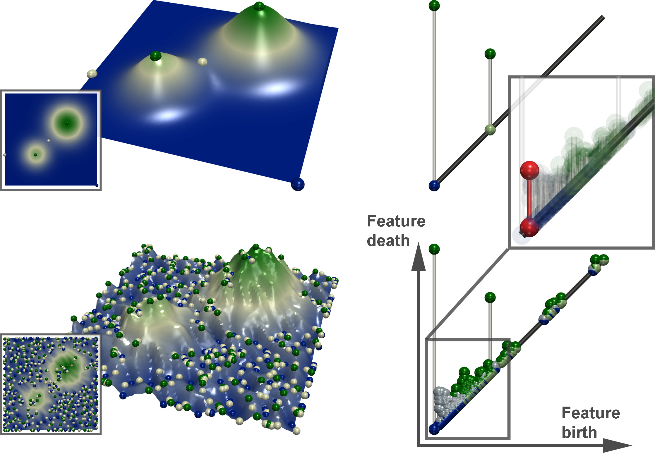
Persistence diagrams: The distribution of critical points of $f$ can be represented visually by a topological abstraction called the persistence diagram [14, 11] (Fig. 1). By applying the Elder Rule [13], critical points can be arranged in a set of pairs, such that each critical point appears in only one pair $(c_{i},c_{j})$ with $f(c_{i})<f(c_{j})$ and $\mathcal{I}(c_{i})=\mathcal{I}(c_{j})-1$. Intuitively, the Elder Rule [13] states that if two topological features of $f^{-1}_{-\infty}(i)$ (for instance two connected components) meet at a given saddle $c_{j}$ of $f$, the youngest of the two features (the one created last) dies at the advantage of the oldest. For example, if two connected components of $f^{-1}_{-\infty}(i)$ merge at a saddle $c_{j}$, the one created by the highest minimum $c_{i}$ (the youngest one) is considered to die at $c_{j}$, and $c_{i}$ and $c_{j}$ will form a critical point pair. The persistence diagram $\mathcal{D}(f)$ embeds each pair $(c_{i},c_{j})$ in the plane such that its horizontal coordinate equals $f(c_{i})$, and the vertical coordinate of $c_{i}$ and $c_{j}$ are $f(c_{i})$ and $f(c_{j})$, corresponding respectively to the birth and death of the pair. The height of the pair $P(c_{i},c_{j})=|f(c_{j})-f(c_{i})|$ is called the persistence and denotes the life-span of the topological feature created in $c_{i}$ and destroyed in $c_{j}$. Thus, features with a short life span (noise) will appear in $\mathcal{D}(f)$ as low persistence pairs near the diagonal (Figure 1, bottom). In low dimension, the persistence of the pairs linking critical points of index $(0,1)$, $((d-1),d)$ and $(1,2)$ (in 3D) denotes the life-span of connected components, voids and non-collapsible cycles of $f^{-1}_{-\infty}(i)$. In the rest of the paper, when discussing persistence diagrams, we will only consider critical point pairs of index $(0,1)$ and $((d-1),d)$. The impact of this simplification is discussed in Sec. 4.4. In practice, persistence diagrams serve as an important visual representation of the distribution of critical points in a scalar data-set. Small oscillations in the data due to noise will typically be represented by critical point pairs with low persistence, in the vicinity of the diagonal. In contrast, topological features that are the most prominent in the data will be associated with large vertical bars (Figure 1). In many applications, persistence diagrams help users as a visual guide to interactively tune simplification thresholds in topology-based, multi-scale data segmentation tasks based on the Reeb graph [9, 34, 45, 19, 42] or the Morse-Smale complex [21, 22].

Distance: In order to evaluate the quality of compression algorithms, several metrics have been defined to evaluate the distance between the decompressed data, noted $g:\mathcal{M}\rightarrow\mathbb{R}$, and the input data, $f:\mathcal{M}\rightarrow\mathbb{R}$. The $p$-norm, noted $||f-g||_{p}$, is a classical example:

$$||f-g||_{p}=\Big{(}\sum_{v\in\mathcal{M}}|f(v)-g(v)|^{p}\Big{)}^{{1}\over{p}}$$ (1)

Typical values of $p$ with practical interests include $p=2$ and $p\rightarrow\infty$. In particular, the latter case, called the maximum norm, is used to estimate the maximum pointwise error:

$$||f-g||_{\infty}=\max_{v\in\mathcal{M}}|f(v)-g(v)|$$ (2)

In the compression literature, a popular metric is the the Peak Signal to Noise Ratio (PSNR), where $|\sigma_{0}|$ is the number of vertices in $\mathcal{M}$:

$$PSNR=20~{}log_{10}\Big{(}{{\sqrt{|\sigma_{0}|}}\over{2}}\times{{\max_{v\in\mathcal{M}}f(v)-\min_{v\in\mathcal{M}}f(v)}\over{||f-g||_{2}}}\Big{)}$$ (3)

Figure 2: Overview of our topologically controlled lossy compression scheme on a 2D elevation example. First the input data $f:\mathcal{M}\rightarrow\mathbb{R}$ is pre-simplified into a function $f^{\prime}$ ((a), from top to bottom) to remove all topological features below a user persistence tolerance $\epsilon$ (as illustrated by the persistence diagram (b)). The compression is achieved by a topologically adaptive quantization of the range, which is segmented along the critical values of $f^{\prime}$ (c). A quantized function $f^{\prime\prime}$ is constructed ((c), bottom) to only use a finite set of possible data values for regular vertices, hence guaranteeing data compression, while still enforcing original values at critical points. This approach can be extended with point wise error control ((d)), by refining each quantization interval of $f^{\prime}$ larger than a target width ((d), bottom). Moreover, our approach can be combined with any third party compressor (e) to further improve the geometry of the compressed data.

In the context of topological data analysis, several metrics [11] have been introduced too, in order to compare persistence diagrams. In our context, such metrics will be instrumental to evaluate the preservation of topological features after decompression. The bottleneck distance [11], noted $d^{B}_{\infty}\big{(}\mathcal{D}(f),\mathcal{D}(g)\big{)}$, is a popular example. Persistence diagrams can be associated with a pointwise distance, noted $d_{\infty}$ inspired by the $\infty$-norm. Given two critical points $p=(p_{x},p_{y})\in\mathcal{D}(f)$ and $q=(q_{x},q_{y})\in\mathcal{D}(g)$, $d_{\infty}$ is defined as:

$$d_{\infty}(p,q)=\max(|p_{x}-q_{x}|,|p_{y}-q_{y}|)$$ (4)

Assume that the number of critical points of all possible index $\mathcal{I}$ is the same in both $\mathcal{D}(f)$ and $\mathcal{D}(g)$. Then the bottleneck distance $d^{B}_{\infty}\big{(}\mathcal{D}(f),\mathcal{D}(g)\big{)}$ can be defined as follows:

$$d^{B}_{\infty}\big{(}\mathcal{D}(f),\mathcal{D}(g)\big{)}=\min_{\phi\in\Phi}\bigg{(}\max_{p\in\mathcal{D}(f)}\Big{(}d_{\infty}\big{(}p,\phi(p)\big{)}\Big{)}\bigg{)}$$ (5)

where $\Phi$ is the set of all possible bijections $\phi$ mapping the critical points of $\mathcal{D}(f)$ to critical points of the same index $\mathcal{I}$ in $\mathcal{D}(g)$. If the numbers of critical points of index $\mathcal{I}$ do not match in both diagrams, $\phi$ will be an injection from the smaller set of critical points to the larger one. Additionally, $\phi$ will collapse the remaining, unmatched, critical points in the larger set by mapping each critical point $c_{i}$ to the other extremity of its persistence pair $c_{j}$, in order to still penalize the presence of unmatched, low persistence features.

Intuitively, in the context of scalar data compression, the bottleneck distance between two persistence diagrams can be usually interpreted as the maximal size of the topological features which have not been maintained through compression (Fig. 1).

A simple variant of the bottleneck distance, that is slightly more informative in the context of data compression, is the Wasserstein distance, noted $d^{W}_{\infty}$ (sometimes called the Earth Mover’s Distance [30]), between the persistence diagrams $\mathcal{D}(f)$ and $\mathcal{D}(g)$:

$$d^{W}_{\infty}\big{(}\mathcal{D}(f),\mathcal{D}(g)\big{)}=\min_{\phi\in\Phi}\bigg{(}\sum_{p\in\mathcal{D}(f)}\Big{(}d_{\infty}\big{(}p,\phi(p)\big{)}\Big{)}\bigg{)}$$ (6)

In contrast to the bottleneck distance, the Wasserstein distance will take into account the persistence of all the pairs which have not been maintained through compression (not only the largest one).

1.2 Overview

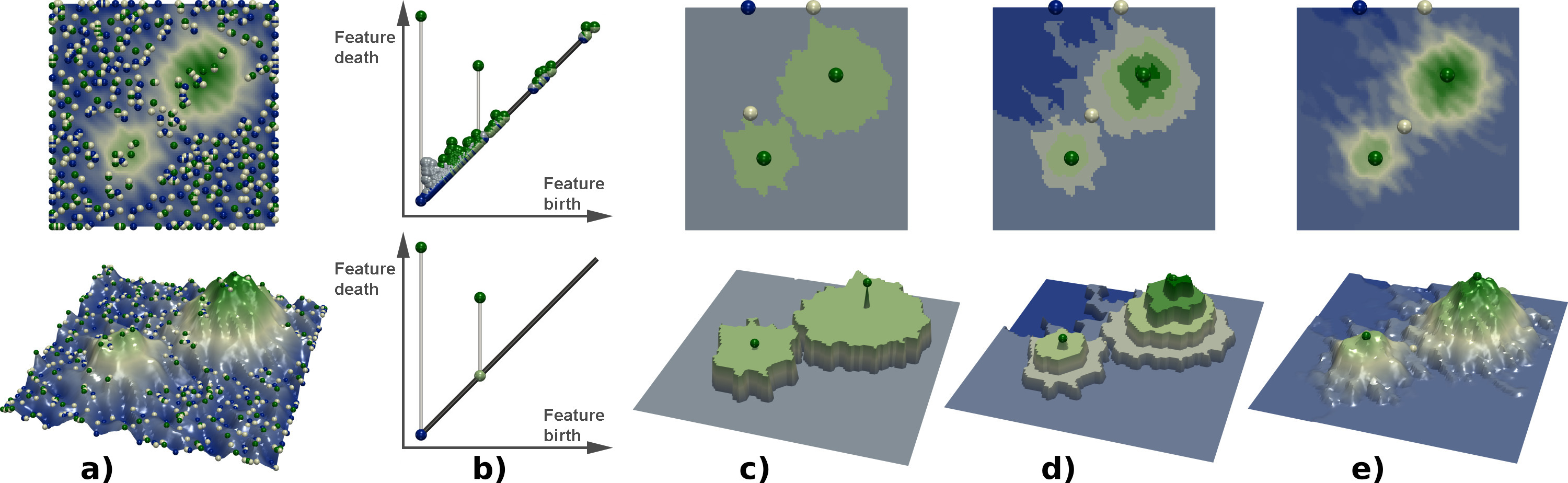
An overview of our compression approach is presented in Fig. 2. First, the persistence diagram of the input data $f:\mathcal{M}\rightarrow\mathbb{R}$ is computed so as to evaluate noisy topological features to later discard. The diagram consists of all critical point pairs of index $(0,1)$ and $(d-1,d)$. Next, given a target size for the preservation of topological features, expressed as a persistence threshold $\epsilon$, a simplified function $f^{\prime}:\mathcal{M}\rightarrow\mathbb{R}$ is reconstructed [46] from the persistence diagram of $f$, $\mathcal{D}(f)$, from which all persistence pairs below $\epsilon$ have been removed (Fig. 2(a)). Next, the image of $\mathcal{M}$, $f^{\prime}(\mathcal{M})$, is segmented along each critical value of $f^{\prime}$. A new function $f^{\prime\prime}:\mathcal{M}\rightarrow\mathbb{R}$ is then obtained from $f^{\prime}$ by assigning to each vertex the mid-value of the interval it maps to. This constitutes a topologically adaptive quantization of the range (Fig. 2(c)). This quantization can optionally be further subdivided to enforce a maximal pointwise error (Fig. 2(d)). At this point, the data can be compressed by storing the list of critical values of $f^{\prime\prime}$ and storing for each vertex the identifier of the interval it maps to. Optionally, the input data $f$can be compressed independently by state-of-the-art compressors, such as ZFP [31] (Fig. 2(e)).

At decompression, a first function $g^{\prime}:\mathcal{M}\rightarrow\mathbb{R}$ is constructed by re-assigning to each vertex the mid-value of the interval it maps to. Optionally, if the data has been compressed with a third-party compressor, such as ZFP [31], at decompression, each vertex value is cropped to the extent of the interval it should map to. Last, a function $g:\mathcal{M}\rightarrow\mathbb{R}$ is reconstructed from the prescribed critical points of $f^{\prime}$ [46], to remove any topological feature resulting from compression artifacts.

2 Data compression

This section presents our topologically controlled compression scheme. In addition to topological control (Sec. 2.1), our approach can optionally support pointwise error control (Sec. 2.3) as well as combinations with existing compressors (Sec. 2.4). The format of the files generated by our compressor is described in Sec. 2.2.

2.1 Topological control

The input of our algorithm is the input data, $f:\mathcal{M}\rightarrow\mathbb{R}$, as well as the size of the topological features to preserve through compression. This size is expressed as a persistence threshold $\epsilon$.

First, the persistence diagram of the input data, noted $\mathcal{D}(f)$ is computed. Next, a simplified version of the input data, noted $f^{\prime}:\mathcal{M}\rightarrow\mathbb{R}$, is constructed such that $f^{\prime}$ admits a persistence diagram which corresponds to that of $f$, but from which the critical point pairs with persistence smaller than $\epsilon$ have been removed. This simplification is achieved by using the algorithm by Tierny and Pascucci [46], which iteratively reconstructs sub-level sets to satisfy topological constraints on the extrema to preserve. In particular, this algorithm is given as constraints the extrema of $f$ to preserve, which are in our current setting the critical points involved in pairs with persistence larger than $\epsilon$. In such a scenario, this algorithm has been shown to reconstruct a function $f^{\prime}$ such that $||f-f^{\prime}||_{\infty}\leq\epsilon$ [46]. At this point, $f^{\prime}$ carries all the necessary topological information that should be preserved through compression.

In order to compress the data, we adopt a strategy based on range quantization. By assigning only a small number $n$ of possible data values on the vertices of $\mathcal{M}$, only $log_{2}(n)$ bits should be required in principle for the storage of each value (instead of 64 for traditional floating point data with double precision). Moreover, encoding the data with a limited number of possible values is known to constitute a highly favorable configuration for post-process lossless compression, which achieves high compression rates for redundant data.

The difficulty in our context is to define a quantization that respects the topology of $f^{\prime}$, as described by its persistence diagram $\mathcal{D}(f^{\prime})$. To do so, we collect all critical values of $f^{\prime}$ and segment the image of $\mathcal{M}$ by $f^{\prime}$, noted $f^{\prime}(\mathcal{M})$, into a set of contiguous intervals $I=\{I_{0},I_{1},\dots I_{n}\}$, all delimited by the critical values of $f^{\prime}$ (Figure 2, second column, top). Next, we create a new function $f^{\prime\prime}:\mathcal{M}\rightarrow\mathbb{R}$, where all critical points of $f^{\prime}$ are maintained at their corresponding critical value and where all regular vertices are assigned to the mid-value of the interval $I_{i}$ they map to. This constitutes a topologically adaptive quantization of the range: only $n$ possible values will be assigned to regular vertices. Note that although we modify data values in the process, the critical vertices of $f^{\prime}$ are still critical vertices (with identical indices) in $f^{\prime\prime}$, as the lower and upper links (Sec. 1.1) of each critical point are preserved by construction.

2.2 Data encoding

The function $f^{\prime\prime}$ is encoded in a two step process. First a topological index is created. This index stores the identifier of each critical vertex of $f^{\prime\prime}$ as well as its critical value, and for each of these, the identifier $i$ of the interval $I_{i}$ immediately above it if and only if some vertices of $\mathcal{M}$ indeed project to $I_{i}$ through $f^{\prime\prime}$. This strategy enables the save of identifiers for empty intervals.

The second step of the encoding focuses on data values of regular vertices of $f^{\prime\prime}$. Each vertex of $\mathcal{M}$ is assigned the identifier $i$ of the interval $I_{i}$ it projects to through $f^{\prime\prime}$. For $n_{v}$ vertices and $n_{i}$ non-empty intervals between $n_{c}$ critical points, we store per-vertex interval identifiers ($n_{v}$ words of $\log_{2}(n_{i})$ bits), critical point positions in a vertex index ($n_{c}$ words of $\log_{2}(n_{v})$ bits), critical types ($n_{c}$ words of $2$ bits) and critical values ($n_{c}$ floats).

Since it uses a finite set of data values, the buffer storing interval assignments for all vertices of $\mathcal{M}$ is highly redundant. Thus, we further compress the data (topological index and interval assignment) with a standard lossless compressor (Bzip2 [38]).

2.3 Pointwise error control

Figure 3: Topologically controlled compression with pointwise error control. When pre-simplifying the input data $f:\mathcal{M}\rightarrow\mathbb{R}$ (left) into $f^{\prime}$ (center), the value variation of each simplified extremum $e$ equals the persistence $P$ of the pair it belongs to, which is bounded by construction by $\epsilon$: $|f(e)-f^{\prime}(e)|=P\leq\epsilon$ [11, 46]. When adding pointwise error control, each interval is subdivided such that its width does not exceed $\epsilon$ (right). Thus, when constructing the quantized function $f^{\prime\prime}$ which maps each vertex to the middle of its interval, each simplified extremum $e$ of $f$ may further move by a snapping distance $s$ to the middle of its interval, which is itself bounded by half the width of the interval ($\epsilon/2$). Thus, $|f(e)-f^{\prime\prime}(e)|=P+s\leq\epsilon+\epsilon/2$.

Our approach has been designed so far to preserve topological features thanks to a topologically adaptive quantization of the range. However, this quantization may be composed of arbitrarily large intervals, which may result in large pointwise error.

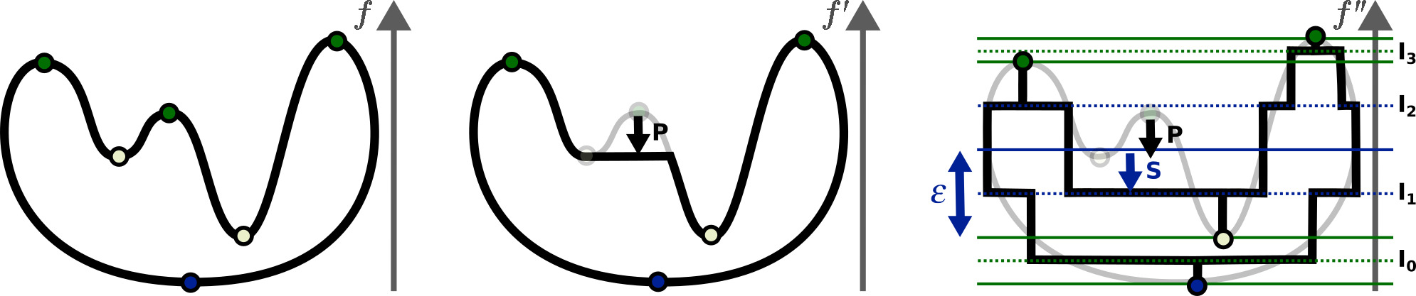
Our strategy can be easily extended to optionally support a maximal pointwise error with regard to the input data $f:\mathcal{M}\rightarrow\mathbb{R}$, still controlled by the parameter $\epsilon$. In particular, this can be achieved by subdividing each interval (Sec. 2.1) according to a target maximal width $w$, prior to the actual quantization and data encoding (Sec. 2.2). Since the topologically simplified function $f^{\prime}$ is guaranteed to be at most $\epsilon$-away from $f$ ($||f-f^{\prime}||_{\infty}\leq\epsilon$, Sec. 2.1), further subdividing each interval with a maximum authorized width of $w$ will result in a maximum error of $\epsilon+w/2$ when quantizing the data into $f^{\prime\prime}$. For instance, a local maximum of $f$ of persistence lower than $\epsilon$ can be pulled down by at most $\epsilon$ when simplifying $f$ into $f^{\prime}$ [46] (Fig. 3, center) and then further pulled down by up to $w/2$ when being assigned the mid-value of its new interval (of width $w$, Fig. 3, right). In practice, for simplicity, we set $w=\epsilon$. Hence, a maximum pointwise error of $3\epsilon/2$ is guaranteed at compression ($||f-f^{\prime\prime}||_{\infty}\leq 3\epsilon/2$).

2.4 Combination with state-of-the-art compressors

The compression approach we presented so far relies on a topologically adaptive quantization of the range (with optional pointwise error control). The compression is achieved by only allowing a small number of possible scalar values in the compressed data, which may typically result in noticeable staircase artifacts. To address this, our method can be optionally combined seamlessly with any state-of-the-art lossy compressor. For our experiments, we used ZFP [31]. Such a combination is straightforward at compression time. In particular, in addition to the topological index and the compressed quanta identifiers (subsection 2.2), the input data $f:\mathcal{M}\rightarrow\mathbb{R}$ is additionally and independently compressed by the third-party compressor (ZFP).

3 Data decompression

This section describes the decompression procedure of our approach, which is symmetric to the compression pipeline described in the previous section (Sec. 2). This section also further details the guarantees provided by our approach regarding the bottleneck ($d^{B}_{\infty}$) and Wasserstein ($d^{W}_{\infty}$) distances between the persistence diagrams of the input data and the decompressed data, noted $g:\mathcal{M}\rightarrow\mathbb{R}$ (Sec. 3.4).

3.1 Data decoding

First, the compressed data is decompressed with the lossless decompressor Bzip2 [38]. Next, a function $g^{\prime}:\mathcal{M}\rightarrow\mathbb{R}$ is constructed based on the topological index and the interval assignment buffer (Sec. 2.2). In particular, each critical vertex is assigned its critical value (as stored in the topological index) and regular vertices are assigned the mid-value of the interval they project to, based on the interval assignment buffer (Sec. 2.2).

3.2 Combination with state-of-the-art decompressors

If a state-of-the-art compression method has been used in conjunction with our approach (Sec. 2.4), we use its decompressor to generate the function $g^{\prime}:\mathcal{M}\rightarrow\mathbb{R}$. Next, for each vertex $v$ of $\mathcal{M}$, if $g^{\prime}(v)$ is outside of the interval $I_{i}$ where $v$ is supposed to project, we snap $g^{\prime}(v)$ to the closest extremity of $I_{i}$. This guarantees that the decompressed data respects the topological constraints of $\mathcal{D}(f^{\prime})$, as well as the optional target pointwise error (Sec. 2.3).

3.3 Topological reconstruction

The decompressed function $g^{\prime}$ may contain at this point extraneous critical point pairs, which were not present in $\mathcal{D}(f^{\prime})$ (Sec. 2.1). For instance, if a state-of-the-art compressor has been used in conjunction with our approach, arbitrary oscillations within a given interval $I_{i}$ can still occur and result in the apparition of critical point pairs in $\mathcal{D}(g^{\prime})$ (with a persistence smaller than the target interval width $w$, Sec. 2.3) which were not present in $\mathcal{D}(f^{\prime})$. The presence of such persistence pairs impacts the distance metrics introduced in Sec. 1.1, and therefore impacts the quality of our topology controlled compression. Thus, such pairs need to be simplified in a post-process.

Note that, even if no third-party compressor has been used, since our approach is based on a topologically adaptive quantization of the range, large flat plateaus will appear in $g^{\prime}$. Depending on the vertex offset $\mathcal{O}_{g^{\prime}}:\mathcal{M}\rightarrow\mathbb{R}$ (used to disambiguate flat plateaus, Sec. 1.1), arbitrarily small persistence pairs can also occur. Therefore, for such flat plateaus, $\mathcal{O}_{g^{\prime}}$ must be simplified to guarantee its monotonicity everywhere except at the desired critical vertices (i.e. those stored in the topological index, Sec. 2.2).

Thus, whether a state-of-the-art compressor has been used or not, the last step of our approach consists in reconstructing the function $g:\mathcal{M}\rightarrow\mathbb{R}$ from $g^{\prime}$ by enforcing the critical point constraints of $f^{\prime}$ (stored in the topological index) with the algorithm by Tierny and Pascucci [46]. Note that this algorithm will automatically resolve flat plateaus, by enforcing the monotonicity of $\mathcal{O}_{g}$ everywhere except at the prescribed critical points [46]. Therefore, the overall output of our decompression procedure is the scalar field $g:\mathcal{M}\rightarrow\mathbb{R}$ as well as its corresponding vertex integer offset $\mathcal{O}_{g}:\mathcal{M}\rightarrow\mathbb{N}$.

Figure 4: Compression of the noisy 2D data set from Fig. 1 ((a), 80,642 bytes, top: 2D data, bottom: 3D terrain). In all cases (c-e), our compression algorithm was configured to maintain topological features more persistent than $20\%$ of the function range, as illustrated with the persistence diagrams ((b), top: original noisy data $\mathcal{D}(f)$, bottom: decompressed data $\mathcal{D}(g)$). Our topology controlled compression (c), augmented with pointwise error control (d), and combined with ZFP [31] ((e), one bit per scalar) yields compression rates of 163, 50 and 14 respectively.

3.4 Topological guarantees

The last step of our decompression scheme, topological reconstruction (Sec. 3.3), guarantees that $\mathcal{D}(g)$ admits no other critical points than those of $\mathcal{D}(f^{\prime})$ (specified in the topological index). Moreover, the corresponding critical values have been strictly enforced (Sec. 3.1). This guarantees that $d^{B}_{\infty}\big{(}\mathcal{D}(g),\mathcal{D}(f^{\prime})\big{)}=0$, and thus:

$$\begin{array}[]{l@{}l}d^{B}_{\infty}\big{(}\mathcal{D}(g),\mathcal{D}(f)\big{)}&{}\leq d^{B}_{\infty}\big{(}\mathcal{D}(g),\mathcal{D}(f^{\prime})\big{)}+d^{B}_{\infty}\big{(}\mathcal{D}(f^{\prime}),\mathcal{D}(f)\big{)}\\ {}&\leq d^{B}_{\infty}\big{(}\mathcal{D}(f^{\prime}),\mathcal{D}(f)\big{)}\end{array}$$ (9)

Since we know that $f^{\prime}$ is $\epsilon$-away from the original data $f$ (Sec. 2.1) and due to persistence diagrams stability [11], we then have:

$$d^{B}_{\infty}\big{(}\mathcal{D}(g),\mathcal{D}(f)\big{)}\leq||f-f^{\prime}||_{\infty}\leq\epsilon$$ (10)

Thus, the bottleneck distance between the persistence diagrams of the input and decompressed data is indeed bounded by $\epsilon$, which happens to precisely describe the size of the topological features that the user wants to preserve through compression.

Since $\mathcal{D}(f^{\prime})\subset\mathcal{D}(f)$ and $d^{B}_{\infty}\big{(}\mathcal{D}(g),\mathcal{D}(f^{\prime})\big{)}=0$, we have $\mathcal{D}(g)\subset\mathcal{D}(f)$. This further implies that:

$$d^{B}_{\infty}\big{(}\mathcal{D}(g),\mathcal{D}(f)\big{)}=\max_{(p,q)\in\big{(}\mathcal{D}(g)\bigtriangleup\mathcal{D}(f)\big{)}}P(p,q)$$ (11)

where $P(p,q)$ denotes the persistence of a critical point pair $(p,q)$ and where $\mathcal{D}(g)\bigtriangleup\mathcal{D}(f)$ denotes the symmetric difference between $\mathcal{D}(g)$ and $\mathcal{D}(f)$ (i.e. the set of pairs present in $\mathcal{D}(f)$ but not in $\mathcal{D}(g)$). In other words, the bottleneck distance between the persistence diagrams of the input and decompressed data exactly equals the persistence of the most persistent pair present in $\mathcal{D}(f)$ but not in $\mathcal{D}(g)$ (in red in Fig. 1). This guarantees the exact preservation of the topological features selected with an $\epsilon$ persistence threshold.

As for the Wasserstein distance, with the same rationale, we get:

$$d^{W}_{\infty}\big{(}\mathcal{D}(g),\mathcal{D}(f)\big{)}=\sum_{(p,q)\in\big{(}\mathcal{D}(g)\bigtriangleup\mathcal{D}(f)\big{)}}P(p,q)$$ (12)

In other words, the Wasserstein distance between the persistence diagrams of the input and decompressed data will be exactly equal to sum of the persistence of all pairs present in $\mathcal{D}(f)$ but not in $\mathcal{D}(g)$ (small bars near the diagonal in Fig. 1, bottom), which corresponds to all the topological features that the user precisely wanted to discard.

Finally, for completeness, we recall that, if pointwise error control was enabled, our approach guarantees $||f-g||_{\infty}\leq 3\epsilon/2$ (Sec. 2.3).

4 Results

This section presents experimental results obtained on a desktop computer with two Xeon CPUs (3.0 GHz, 4 cores each), with 64 GB of RAM. For the computation of the persistence diagram and the topological simplification of the data, we used the algorithms by Tierny and Pascucci [46] and Gueunet et al. [20], whose implementations are available in the Topology ToolKit (TTK) [43]. The other components of our approach (including bottleneck and Wasserstein distance computations) have been implemented as TTK modules. Note that our approach has been described so far for triangulations. However, we restrict our experiments to regular grids in the following as most state-of-the-art compressors (including ZFP [31]) have been specifically designed for regular grids. For this, we use the triangulation data-structure from TTK, which represents implicitly regular grids with no memory overhead using a 6-tet subdivision.

Fig. 4 presents an overview of the compression capabilities of our approach on a noisy 2D example. A noisy data set is provided on the input. Given a user threshold on the size of the topological features to preserve, expressed as a persistence threshold $\epsilon$, our approach generates decompressed data-sets that all share the same persistence diagram $\mathcal{D}(g)$ (Figure 4(b), bottom), which is a subset of the diagram of the input data $\mathcal{D}(f)$ (Figure 4(b), top) from which pairs with a persistence lower than $\epsilon$ have been removed, and those above $\epsilon$ have been exactly preserved. As shown in this example, augmenting our approach with pointwise error control or combining it with a state-of-the-art compressor allows for improved geometrical reconstructions, but at the expense of much lower compression rates. Note that the Figure 4(e) shows the result of the compression with ZFP [31], which has been augmented with our topological control. This shows that our approach can enhance any existing compression scheme, by providing strong topological guarantees on the output.

4.1 Compression performance

We first evaluate the performance of our compression scheme with topological control only on a variety of 3D data sets all sampled on $512^{3}$ regular grids. Fig. 5 (left) presents the evolution of the compression rates for increasing target persistence thresholds $\epsilon$ expressed as percentages of the data range. This plot confirms that when fine scale structures need to be preserved (small $\epsilon$ values, left), smaller compression rates are achieved, while higher compression rates (right) are reached when this constraint is relaxed. Compression rates vary among data sets as the persistence diagrams vary in complexity. The Ethane Diol dataset (topmost curve) is a very smooth function coming from chemical simulations. High compression factors are achieved for it, almost irrespective of $\epsilon$. On the contrary, the random dataset (bottom curve) exhibits a complex persistence diagram, and hence lower compression rates.

In between, all data sets exhibit the same increase in compression rate for increasing $\epsilon$ values. Their respective position between the two extreme configurations of the spectrum (elevation and random) depend on their input topological complexity (number of pairs in the persistence diagram).

Figure 5: Performance analysis of our compression scheme (topological control only). Left: Compression rate for various 3D data sets, as a function of the target persistence threshold $\epsilon$ (percentage of the function range). Right: Bottleneck distance between the persistence diagrams of the input and decompressed data, $d^{B}_{\infty}\big{(}\mathcal{D}(f),\mathcal{D}(g)\big{)}$, for increasing target persistence thresholds $\epsilon$.

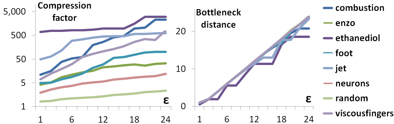
Fig. 5 (right) plots the evolution of the bottleneck distance between the input and decompressed data, $d^{B}_{\infty}\big{(}\mathcal{D}(f),\mathcal{D}(g)\big{)}$, for increasing target persistence threshold $\epsilon$, for all data sets. This plot shows that all curves are located below the identity diagonal. This constitutes a practical validation of our guaranteed bound on the bottleneck distance (Eq. 10). Note that, for a given data set, the proximity of its curve to the diagonal is directly dependent on its topological complexity. This result confirms the strong guarantees regarding the preservation of topological features through compression.

Table 1: Detailed computation times on $512^{3}$ regular grids ($\epsilon=5\%$), with and without compression-time simplification. $P$, $S$, $Q$ and $L$ stand for the persistence diagram, topological simplification, topological quantization and lossless compression efforts (%).

Data-set	With compression-time simplification						No simplification		Decompr.
	P (%)	S (%)	Q (%)	L (%)	Total (s)	Compr. Rate	Total (s)	Compr. Rate	Time (s)
Combustion	8.4	89.3	0.7	1.6	593.9	121.3	64.1	111.1	213.3
Elevation	14.6	84.1	1.2	0.1	157.0	174,848.0	25.3	174,848.0	211.5
EthaneDiol	12.6	86.7	0.5	0.2	490.0	2,158.6	63.0	2,158.6	228.9
Enzo	9.5	86.7	1.0	2.7	695.6	24.5	91.8	19.8	204.0
Foot	12.6	81.9	1.6	3.8	380.6	12.1	68.4	7.75	205.7
Jet	22.2	75.7	0.6	1.5	451.3	315.6	111.1	287.6	220.3
Random	15.9	76.0	2.8	5.3	1357.1	1.5	307.7	1.5	101.2

Table 1 provides detailed timings for our approach and shows that most of the compression time (at least 75%, $S$ column) is spent simplifying the original data $f$ into $f^{\prime}$ (section 2). If desired, this step can be skipped to drastically improve time performance, but at the expense of compression rates (Table 1, right). Indeed, as shown in Figure 6, skipping this simplification step at compression time results in quantized function $f^{\prime\prime}$ that still admits a rich topology, and which therefore constitutes a less favorable ground for the post-process lossless compression (higher entropy). Note however that our implementation has not been optimized for execution time. We leave time performance improvement for future work.

Figure 6: Topologically controlled compression with (b) and without (c) compression-time simplification. Topological simplification (c to d) removes all critical point pairs not present in the topological index (red circles) and exactly maintains the others [46]. Thus, simplifying the data only at decompression (d) yields identical decompressed data (d vs b). The quantized function then admits a richer topology (c vs b), which deteriorates compression rates.

4.2 Comparisons

Figure 7: Comparison to the SQ compressor [27] (green: SQ-D, blue: SQ-R, red: our approach). Left: average normalized Wasserstein distance between the persistence diagrams of the input and decompressed data, for increasing compression rates. Right: average compression factors for increasing target persistence thresholds $\epsilon$.

Next, we compare our approach with topological control only to the SQ compressor [27], which has been explicitly designed to control pointwise error. Thus, it is probably the compression scheme that is the most related to our approach. SQ proposes two main strategies for data compression, one which is a straight range quantization (with a constant step size $\epsilon$, SQ-R) and the other which grows regions in the 3D domain, within a target function interval width $\epsilon$ (SQ-D). Both variants, which we implemented ourselves, provide an explicit control on the resulting pointwise error ($||f-g||_{\infty}\leq\epsilon$). As such, thanks to the stability result on persistence diagrams [11], SQ also bounds the bottleneck distance between the persistence diagrams of the input and decompressed data. Each pair completely included within one quantization step is indeed flattened out. Only the pairs larger than the quantization step size $\epsilon$ do survive through compression. However, the latter are snapped to admitted quantization values. In practice, this can artificially and arbitrarily reduce the persistence of certain pairs, and increase the persistence of others. This is particularly problematic as it can reduce the persistence of important features and increase that of noise, which prevents a reliable multi-scale analysis after decompression. This difficulty is one of the main motivations which led us to design our approach.

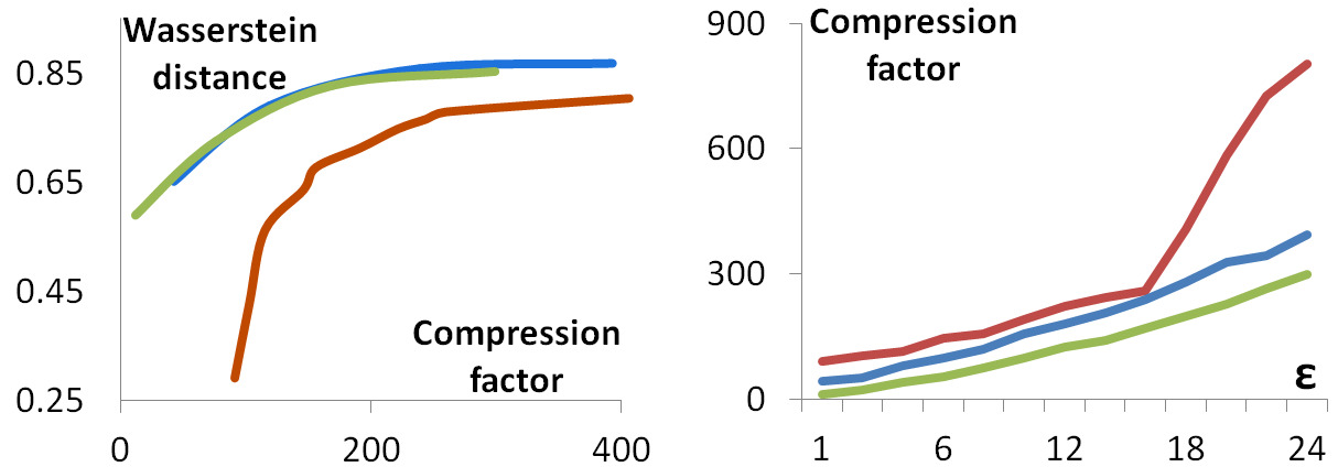
To evaluate this, we compare SQ to our approach in the light of the Wasserstein distance between the persistence diagrams of the input and decompressed data, $d^{W}_{\infty}\big{(}\mathcal{D}(f),\mathcal{D}(g)\big{)}$. As described in Sec. 1.1, this distance is more informative in the context of compression, since not only does it track all pairs which have been lost, but also the changes of the pairs which have been preserved. Fig. 7 (left) presents the evolution of the Wasssertein distance, averaged over all our data sets, for increasing compression rates. This plot shows that our approach (red curve) achieves a significantly better preservation of the topological features than SQ, for all compression rates, especially for the lowest ones. As discussed in the previous paragraph, given a quantization step $\epsilon$, SQ will preserve all pairs more persistent than $\epsilon$ but it will also degrade them, as shown in the above experiment. Another drawback of SQ regarding the preservation of topological features is the compression rate. Since it uses a constant quantization step size, it may require many quantization intervals to preserve pairs above a target persistence $\epsilon$, although large portions of the range may be devoid of important topological features. To illustrate this, we compare the compression rates achieved by SQ and our approach, for increasing values of the parameter $\epsilon$. As in Fig. 5, increasing slopes can be observed. However, our approach always achieves higher compression rates, especially for larger persistence targets.

Figure 8: Augmenting a third party compressor, here ZFP [31] (1 bit per vertex value), with topological control. Left: Compression factors for increasing persistence targets $\epsilon$. Right: PSNR for increasing persistence targets $\epsilon$. In these plots (left and right), a persistence target of $100\%$ indicates that no topological control was enforced.

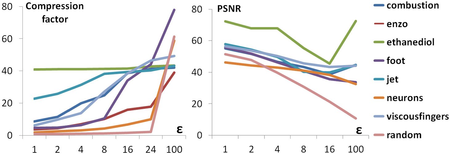
Next, we study the capabilities offered by our approach to augment a third party compressor with topological control (Secs. 2.4 and 3.2). In particular, we augmented the ZFP compressor [31], by using the original implementation provided by the author (with 1 bit per vertex value). Fig. 8 (left) indicates the evolution of the compression rates as the target persistence threshold $\epsilon$ increases. In particular, in these experiments, a persistence target of $100\%$ indicates that no topological control was enforced. Thus, these curves indicate, apart from this point, the overhead of topological guarantees over the ZFP compressor in terms of data storage. These curves, as it could be expected with Fig. 5, show that compression rates will rapidly drop down for topologically rich data sets (such as the random one). On the contrary, for smoother data sets, such as Ethane Diol or Jet, high compression rates can be maintained. This shows that augmenting a third party compressor with topological control results in compression rates that adapt to the topological complexity of the input. Fig. 8 (right) shows the evolution of the PSNR (Sec. 1.1) for decreasing persistence targets $\epsilon$. Surprisingly, in this context, the enforcement of topological control improves the quality of the data decompressed with ZFP, with higher PSNR values for little persistence targets. This is due to the rather aggressive compression rate which we used for ZFP (1 bit per vertex value) which tends to add noise to the data. Thanks to our topological control (Sec. 3.3), such compression artifacts can be cleaned up by our approach.

Table 2 evaluates the advantage of our topology aware compression over a standard lossy compression, followed at decompression by a topological cleanup (which simplifies all pairs less persistent than $\epsilon$ [46]). In particular, this table shows that augmenting a third party compressor (such as ZFP) with our topological control (second line) results in more faithful decompressed data (lower Wasserstein distances to the original data) than simply executing the compressor and topologically cleaning the data in a post-process after decompression (first line). This further motivates our approach for augmenting existing compressors with topological control.

Table 2: Wasserstein distance between the persistence diagrams of the original and decompressed data ($\epsilon=1\%$). First line: ZFP 1bit/scalar, followed by a topology cleanup procedure. Second line: ZFP 1bit/scalar, augmented with our approach.

Data-set	$d^{W}_{\infty}$
	Combustion	Elevation	EthaneDiol	Enzo	Foot	Jet
ZFP + Cleanup	18.08	0.00	1.53	189.66	520,371	351.97
Topology-aware ZFP	13.73	0.00	0.40	131.11	506,714	153.45

Finally, Table 3 provides a comparison of the running times (for comparable compression rates) between our approach and SQ and ZFP. ZFP has been designed to achieve high throughput and thus delivers the best time performances. The running times of our approach are on par with other approaches enforcing strong guarantees on the decompressed data (SQ-R and SQ-D).

Table 3: Time performance comparison between ZFP, SQ and our approach on $512^{3}$ regular grids.

Data-set	Time (s).
	ZFP	SQ-R	SQ-D	Ours
Combustion	4.6	37.6	242.9	64.1
Elevation	7.2	31.4	204.2	25.3
EthaneDiol	4.7	34.4	197.1	63.0
Enzo	4.7	33.0	229.5	91.8
Foot	2.9	18.2	198.0	68.4
Jet	4.7	31.4	203.4	111.1
Random	4.1	31.6	182.7	307.7

4.3 Application to post-hoc topological data analysis

Figure 9: Topology driven data segmentation with multi-scale split trees, on the original data (left) and the data compressed with our approach (right). Top to bottom: persistence diagrams, sliced views of the data, output segmentations. The analysis yields compatible outcomes with and without compression, as shown with the bottom row, which exhibits identical segmentations (compression rate: 360).

A key motivation to our compression scheme is to allow users to faithfully conduct advanced topological data analysis in a post-process, on the decompressed data, with guarantees on the compatibility between the outcome of their analysis and that of the same analysis on the original data. We illustrate this aspect in this sub-section, where all examples have been compressed by our algorithm, without pointwise error control nor combination with ZFP.

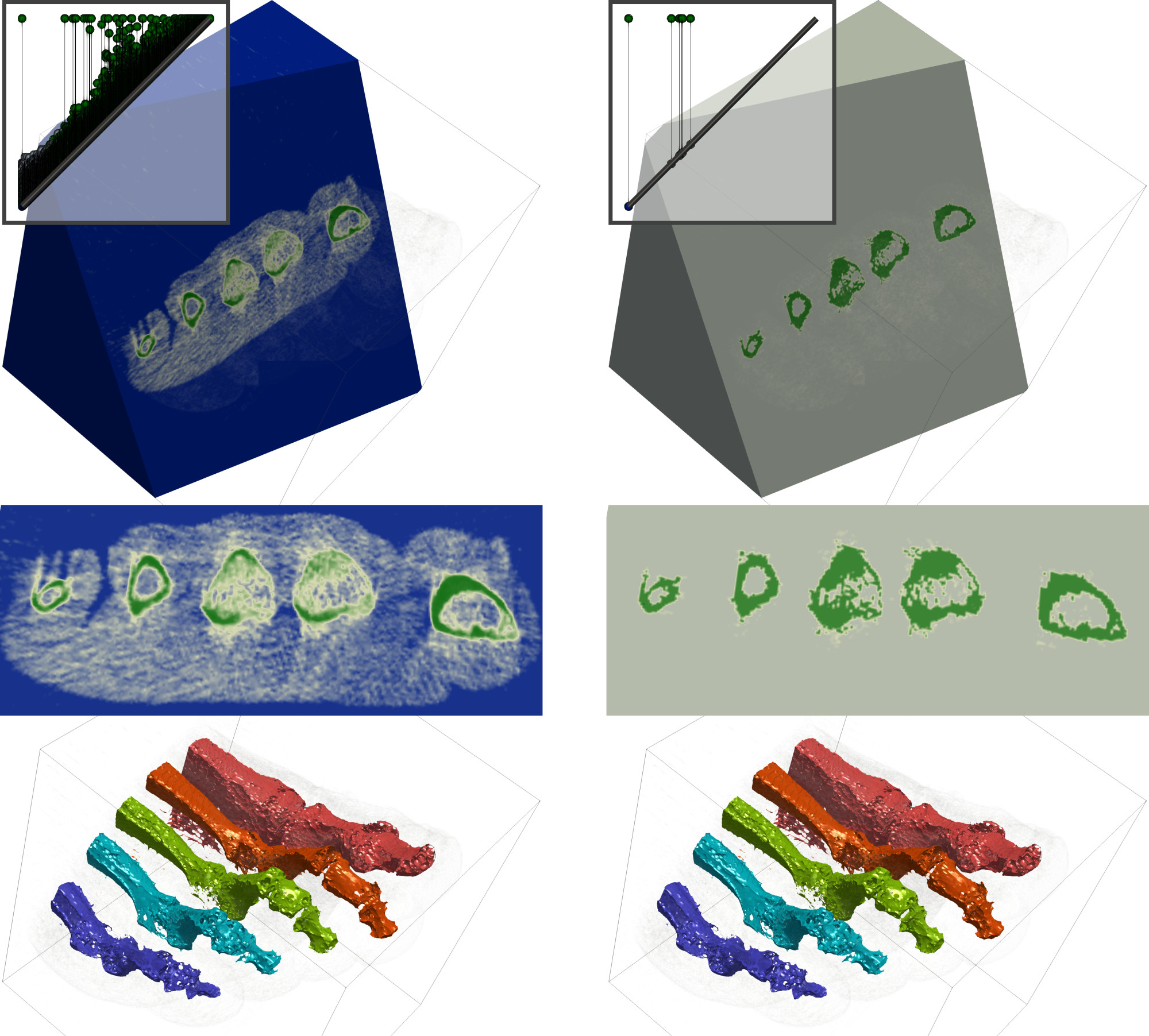
We first illustrate this in the context of medical data segmentation with Fig. 9, which shows a foot scan. The persistence diagram of the original data counts more than 345 thousands pairs (top left). The split tree [5, 8] is a topological abstraction which tracks the connected components of sur-level sets of the data. It has been shown to excel at segmenting medical data [9]. In this context, users typically compute multi-scale simplifications of the split tree to extract the most important features. Here, the user simplified the split tree until it counted only 5 leaves, corresponding to 5 features of interest (i.e. the 5 toes). Next, the segmentation induced by the simplified split tree has been extracted by considering regions corresponding to each arc connected to a leaf. This results immediately in the sharp segmentation of toe bones. (Fig. 9, bottom left). We applied the exact same analysis pipeline on the data compressed with our approach. In particular, since it can be known a priori that this data has only 5 features of interest (5 toes), we compressed the data with a target persistence $\epsilon$ such that only 5 pairs remained in the persistence diagram (top right). Although such an aggressive compression greatly modifies data values, the outcome of the segmentation is identical (Table 4), for an approximate compression rate of 360.

Figure 10: Topology driven data segmentation (right) on a viscous fingering simulation (left) on the original data (top) and the data compressed with our approach. Compatible fingers are extracted after compression (compression rate: 56).

Next, we evaluate our approach on a more challenging pipeline (Fig. 10), where features of interest are not explicitly related to the persistence diagram of the input data. We consider a snapshot of a simulation run of viscous fingering and apply the topological data analysis pipeline described by Favelier et al. [16] for the extraction and tracking of viscous fingers. This pipeline first isolates the largest connected component of sur-level set of salt concentration. Next it considers its height function, on which persistent homology is applied to retrieve the deepest points of the geometry (corresponding to finger tips). Finally, a distance field is grown from the finger tips and the Morse complex of this distance field is computed to isolate fingers. In contrast to the previous example, the original data undergoes many transformations and changes of representation before the extraction of topological features. Despite this, when applied to the data compressed with our scheme, the analysis pipeline still outputs consistent results with the original data (Fig. 10, compression rate: 56). Only slight variations can be perceived in the local geometry of fingers, but their number is unchanged and their overall geometry compatible. Table 4 provides a quantitative estimation of the similarity between segmentations, before and after compression with several algorithms. This table shows that our approach enables the computation of more faithful topological segmentations (higher rand index) compared to SQ and ZFP, which further underlines the superiority of our strategy at preserving topological features.

Table 4: Rand index between the outputs of a data segmentation pipeline based on topological methods (subsection 4.3), before and after compression, for several methods at compatible compression rates.

Experiment	Rand index
	Ours	SQ-R	SQ-D	ZFP
Foot scan	1.000	0.913	0.895	0.943
Viscous fingers	0.985	0.977	0.977	0.973

4.4 Limitations

Like all lossy techniques, our approach is subject to an input parameter that controls the loss, namely the persistence threshold $\epsilon$ above which features should be strictly preserved. While we believe this parameter to be intuitive, prior domain knowledge about the size of the features to preserve may be required. However, conservative values (typically $5\%$) can be used by default, as they already achieve high compression rates while preserving most of the features. In some applications, ad-hoc metrics [9] may be preferred over persistence. Our approach can be used in this setting too as the simplification algorithm that we use [46] supports an arbitrary selection of the critical points to preserve. However, it becomes more difficult then to express clear guarantees on the compression quality in terms of the bottleneck and Wasserstein distances between the persistence diagrams of the input and decompressed data. When pointwise error control is enabled, the $\infty$-norm between the input and decompressed data is guaranteed by our approach to be bounded by $3\epsilon/2$. This is due to the topological simplification algorithm that we employ [46], which is a flooding-only algorithm. Alternatives combining flooding and carving [4, 44] could be considered to reach a guaranteed $\infty$-norm of $\epsilon$. Finally, our approach only considers persistence pairs corresponding to critical points of index $(0,1)$ and (d-1, d). However $(1,2)$ pairs may have a practical interest in certain 3D applications and it might be interesting to enforce their preservation throughout compression. This would require an efficient data reconstruction algorithm for $(1,2)$ pairs, which seems challenging [1].

5 Conclusion

In this paper, we presented the first compression scheme, to the best of our knowledge, which provides strong topological guarantees on the decompressed data. In particular, given a target topological feature size to preserve, expressed as a persistence threshold $\epsilon$, our approach discards all persistence pairs below $\epsilon$ in order to achieve high compression rates, while exactly preserving persistence pairs above $\epsilon$. Guarantees are given on the bottleneck and Wasserstein distances between the persistence diagrams of the input and decompressed data. Such guarantees are key to ensure the reliability of any post-hoc, possibly multi-scale, topological data analysis performed on decompressed data. Our approach is simple to implement; we provide a lightweight VTK-based C++ reference implementation.

Experiments demonstrated the superiority of our approach in terms of topological feature preservation in comparison to existing compressors, for comparable compression rates. Our approach can be extended to include pointwise error control. Further, we showed, with the example of the ZFP compressor [31], how to make any third-party compressor become topology-aware by combining it with our approach and making it benefit from our strong topological guarantees, without affecting too much isosurface geometry. We also showed that, when aggressive compression rates were selected, our topological approach could improve existing compressors in terms of PSNR by cleaning up topological compression artifacts. We finally showed the utility of our approach by illustrating, qualitatively and quantitatively, the compatibility between the output of post-hoc topological data analysis pipelines, executed on the input and decompressed data, for simulated or acquired data sets. Our contribution enables users to faithfully conduct advanced topological data analysis on decompressed data, with guarantees on the size of missed features and the exact preservation of most prominent ones.

In the future, we plan to improve practical aspects of our algorithm for in-situ deployment and to handle time-varying datasets. Runtime limitations will be investigated, with the objective to mitigate the effects of using (or not) a sequential topological simplification step, and to determine how many cores are necessary to outperform raw storage. A streaming version of the algorihm, which would not require the whole dataset to be loaded at once would be of great interest in this framework. Finally, as our approach focuses on regular grids, since, in the case of unstructured grids, the actual mesh is often the information that requires the most storage space, we will investigate mesh compression techniques with guarantees on topological feature preservation for scalar fields defined on them.