A strongly interacting Sarma superfluid near orbital Feshbach resonances

Abstract

We investigate the nature of superfluid pairing in a strongly interacting Fermi gas near orbital Feshbach resonances with spin-population imbalance in three dimensions, which can be well described by a two-band or two-channel model. We show that a Sarma superfluid with gapless single-particle excitations is favored in the closed channel at large imbalance. It is thermodynamically stable against the formation of an inhomogeneous Fulde–Ferrell–Larkin–Ovchinnikov superfluid and features a well-defined Goldstone-Anderson-Bogoliubov phonon mode and a massive Leggett mode as collective excitations at low momentum. At large momentum, the Leggett mode disappears and the phonon mode becomes damped at zero temperature, due to the coupling to the particle-hole excitations. We discuss possible experimental observation of a strongly interacting Sarma superfluid with ultracold alkaline-earth-metal Fermi gases.

I Introduction

A Sarma phase, named after the pioneering work by Sarma in 1963 Sarma1963 , is a possible candidate state for a homogeneous Fermi superfluid with pair-breaking population imbalance. Having gapless fermionic excitations, this state can be conveniently viewed as a phase separation phase in momentum space: some fermions pair and form a superfluid, while others occupy in certain regions of momentum space bounded by gapless Fermi surfaces and remain unpaired. For this reason, the Sarma phase is also vividly referred to as an interior-gap superfluid Liu2003 ; Wu2003 or a breached-pair superfluid Forbes2005 . Although the Sarma phase was predicted more than 50 years ago, its experimental observation remains elusive, in spite of enormous efforts both experimentally and theoretically (for recent reviews, see, for example, Refs. Radzihovsky2010 ; Chevy2010 ; Gubbels2013 ; Kinnunen2017 ). In the original proposal Sarma1963 , the Sarma phase is a local maximum solution in the landscape of the grand thermodynamic potential and suffers from the instability Wu2003 towards a more stable phase-separation phase in real space Bedaque2003 or a spatially inhomogeneous Fulde–Ferrell–Larkin–Ovchinnikov (FFLO) superfluid Fulde1964 ; Larkin1964 . The realization of a thermodynamically stable Sarma phase therefore becomes a long-standing quest Boettcher2015PLB .

The recent intensive research interests on the Sarma phase are largely triggered by the bold proposition by Liu and Wilczek Liu2003 and by the rapid experimental progress in ultracold atomic Fermi gases Zwierlein2006 ; Partridge2006 ; Liao2010 . It has been now realized that, to cure the instability of the Sarma phase, one needs to carefully engineer the inter-particle interactions and/or the mass ratio of the different spin components Forbes2005 ; Parish2007 ; Baarsma2010 ; Wang2017 . In the context of two-component spin-1/2 atomic Fermi gases at the crossover from a Bose-Einstein condensation (BEC) to a Bardeen-Cooper-Schrieffer (BCS) superfluid Bloch2008 ; Giorgini2008 ; Randeria2014 , the Sarma phase becomes stable on the BEC side of a BEC-BCS crossover Sheehy2006 ; Sheehy2007 ; Hu2006PRA , featuring one gapless Fermi surface and behaving similar to a Bose-Fermi mixture. A large mass ratio may greatly enlarge the phase space of the Sarma phase, making it energetically favorable even at the cusp of the BEC-BCS crossover Parish2007 ; Baarsma2010 ; Wang2017 , the so-called unitary limit. In this respect, heteronuclear Fermi-Fermi mixtures of ⁶Li-⁴⁰K, ⁶Li-⁸⁷Sr and ⁶Li-¹⁷³Yb atoms look very promising, although there are still some technical issues related to atom loss and temperature cooling. Interestingly, the Sarma phase may also be stabilized by considering a multi-band structure. In an early study He2009 , one of the present authors showed that in a two-band Fermi system with four spin components, the inter-band exchange interaction together with asymmetric intra-band interactions can remove the Sarma instability and the Sarma phase could be the energetically stable ground state in visible parameter space. It is then natural to ask, can we realize this kind of two-band proposal with ultracold atoms?

This possibility may come to true, thanks to the recent innovative proposal by Zhang, Cheng, Zhai and Zhang Zhang2015 , named as orbital Feshbach resonance (OFR), which has been confirmed soon experimentally Pagano2015 ; Hofer2015 . In Fermi gases of alkali-earth metal atoms (i.e., Sr) or alkali-earth metal like atoms (i.e., Yb), the long-lived meta-stable orbital (i.e., electronic) state ${}^{3}P_{0}$ (denoted as $\left|e\sigma\right\rangle$ where $\sigma=\uparrow,\downarrow$ stands for the two internal nuclear spin states) can be selected, together with the ground orbital state ${}^{1}S_{0}$ ($\left|g\sigma\right\rangle$). This forms an effective four-component Fermi system, in which a pair of atoms can be well described by using the singlet ($-$) and triplet ($+$) basis in the absence of external Zeeman field Zhang2015 ; Pagano2015 ; Hofer2015 ; He2016 ,

$$\left|\pm\right\rangle=\frac{1}{2}\left(\left|ge\right\rangle\pm\left|eg\right\rangle\right)\otimes\left(\left|\uparrow\downarrow\right\rangle\mp\left|\downarrow\uparrow\right\rangle\right),$$ (1)

or by using the two-channel basis in the presence of Zeeman field Zhang2015 ; Pagano2015 ; Hofer2015 ; He2016 ,

$$\left|o\right\rangle = \frac{1}{\sqrt{2}}\left(\left|-\right\rangle+\left|+\right\rangle\right)=\frac{1}{\sqrt{2}}\left(\left|g\uparrow,e\downarrow\right\rangle-\left|e\downarrow,g\uparrow\right\rangle\right),$$ (2)

$$\left|c\right\rangle = \frac{1}{\sqrt{2}}\left(\left|-\right\rangle-\left|+\right\rangle\right)=\frac{1}{\sqrt{2}}\left(\left|g\downarrow,e\uparrow\right\rangle-\left|e\uparrow,g\downarrow\right\rangle\right),$$ (3)

where $o$ and $c$ stand for the open and closed channels, respectively. The inter-particle interactions are characterized by two underlying $s$-wave scattering lengths, the singlet scattering length $a_{s-}$ and the triplet scattering length $a_{s+}$, whose magnitude depend on the atomic species. For ¹⁷³Yb atoms, the triplet scattering length is very large $a_{s+}\simeq 1900a_{0}$ Pagano2015 ; Hofer2015 , where $a_{0}$ is the Bohr radius. It drives the system into the strongly interacting regime and also allows one to tune the effective inter-particle interactions in the open channel via the external Zeeman field Zhang2015 , which thereby realizes the OFR. It turns out that a Fermi gas near OFR can be microscopically described by the two-band theory with a specific form of the interaction Hamiltonian Zhang2015 ; He2016 ; He2015TwoBandTheory . To date, a number of many-body effects of a balanced Fermi gas near OFR have been addressed, including the internal Josephson effect Iskin2016 , critical temperature Xu2016 , stability He2016 ; Iskin2016 , equations of state He2016 , collective modes He2016 ; Zhang2017 , superfluid properties in a harmonic trap Iskin2017 and most recently the closed-channel contributions Mondal2017 . The polaron physics in the limit of extreme spin-population imbalance has also been considered Chen2016 ; Xu2017 ; Chen2018 .

In this work, we would like to confirm the existence of an energetically stable Sarma superfluid near OFR in three dimensions. This is by no means obvious from the previous work He2009 , since the intra-band interaction potentials are now symmetric within OFR. We also explicitly explore the stability of the Sarma superfluid against an inhomogeneous FFLO superfluid. Moreover, for a possible experimental observation, we consider the zero-temperature collective modes of the Sarma superfluid and show the existence of a well-defined Leggett mode Leggett1966 at low momentum and also a damped Goldstone-Anderson-Bogoliubov phonon mode at large momentum (due to the coupling to the particle-hole excitations near the gapless Fermi surface), both of which can be experimentally probed by using Bragg spectroscopy Lingham2014 .

The rest of the paper is organized as follows. In the next section (Sec. II), we introduce the microscopic model of a three-dimensional strongly interacting Fermi gas near OFR with spin-population imbalance and outline the mean-field approach to treat different candidate phases for imbalanced superfluidity, including the Sarma phase and the FFLO phase. In Sec. III, we examine different imbalanced superfluid states and show that the Sarma phase is energetically favorable in certain parameter space. We determine the phase diagram as a function of the chemical potential difference, for the two cases with a fixed chemical potential and with a fixed total number of atoms. In Sec. IV, we consider the Gaussian pair fluctuations on top of the mean-field saddle-point solution and calculate the Green function of Cooper pairs, from which we determine the collective modes of either the gapless phonon mode or the massive Leggett mode. The collective modes of a BCS superfluid and a Sarma superfluid are explored in a comparative way. The discussions of the two-particle continuum and the particle-hole continuum of a Sarma superfluid are given in Appendix A and Appendix B, respectively. Finally, in Sec. V we draw our conclusions.

II Model Hamiltonian

We start by an appropriate description of the interaction Hamiltonian for a Fermi gas near OFR. In the singlet and triplet basis, the interaction potentials between a pair of atoms can be well approximated by using pseudo-potentials Zhang2015 ; He2016 ,

$$V_{\pm}(r)\simeq\frac{4\pi\hbar^{2}a_{s\pm}}{M}\delta(\mathbf{r})\frac{\partial}{\partial r}\left(r\cdot\right),$$ (4)

where $M$ is the mass of fermionic atoms. As we use the external Zeeman field as a control knot, it is convenient to use the two-channel description, in which, following the basis transform of Eq. (2) and Eq. (3), the interaction potentials become

$$V_{oo}(r) = V_{cc}(r)=\frac{V_{-}+V_{+}}{2}=\frac{4\pi\hbar^{2}a_{s0}}{M}\delta(\mathbf{r})\frac{\partial}{\partial r}\left(r\cdot\right),$$ (5)

$$V_{oc}(r) = V_{co}\left(r\right)=\frac{V_{-}-V_{+}}{2}=\frac{4\pi\hbar^{2}a_{s1}}{M}\delta(\mathbf{r})\frac{\partial}{\partial r}\left(r\cdot\right).$$ (6)

The two scattering lengths $a_{s0}$ and $a_{s1}$ are given by, $a_{s0}=(a_{s-}+a_{s+})/2$ and $a_{s1}=(a_{s-}-a_{s+})/2$. The above interaction potentials can be further replaced with contact potentials, $V_{nm}(r)=V_{nm}\delta(\mathbf{r})$, with the bare interaction strengths $V_{nm}$ ($n,m=o,c$) to be renormalized using the two scattering lengths $a_{s0}$ and $a_{s1}$, following the standard renormalization procedure He2016 :

$$\left(\begin{array}[]{cc}V_{oo}&V_{oc}\\ V_{co}&V_{cc}\end{array}\right)^{-1}=\frac{M}{4\pi\hbar^{2}}\left(\begin{array}[]{cc}a_{0}&a_{1}\\ a_{1}&a_{0}\end{array}\right)^{-1}-\sum_{\mathbf{k}}\frac{M}{\hbar^{2}\mathbf{k}^{2}}.$$ (7)

It is then straightforward to write down the interaction Hamiltonian He2016 ,

$$\mathcal{H}_{\textrm{int}}=\sum_{nm}\int d\mathbf{r}V_{nm}\varphi_{n}^{\dagger}\left(\mathbf{r}\right)\varphi_{m}\left(\mathbf{r}\right),$$ (8)

where $\varphi_{n}(\mathbf{r})\equiv\psi_{n2}(\mathbf{r})\psi_{n1}(\mathbf{r})$ is the field operator of annihilating a pair of atoms in the channel $n$. For clarity, we use the subscript $i=1,2$ to denote the two internal degrees of freedom in each channel, instead of using the spin index $\sigma$.

The single-particle Hamiltonian in three dimensional free space takes the standard form Zhang2015 ; He2016 ,

$$\mathcal{H}_{0}=\sum_{ni}\int d\mathbf{r}\psi_{ni}^{\dagger}\left(\mathbf{r}\right)\left(-\frac{\hbar^{2}\nabla^{2}}{2M}-\mu_{ni}\right)\psi_{ni}\left(\mathbf{r}\right),$$ (9)

where for the channel $n=(o,c)$, we assume $\mu_{n1}=\mu_{n}+\delta\mu_{n}$ and $\mu_{n2}=\mu_{n}-\delta\mu_{n}$. In the presence of a Zeeman field, a pair of atoms in the open and closed channels has different Zeeman energy with a difference, $\delta(B)=(g_{g}m_{\downarrow}+g_{e}m_{\uparrow})\mu_{B}B-(g_{g}m_{\uparrow}+g_{e}m_{\downarrow})\mu_{B}B$, arising from the difference in their magnetic momentum (see Eq. (2) and Eq. (3)). As a result, we may define the effective chemical potentials of the open and closed channels as, $\mu_{o}=\mu$ and

$$\mu_{c}=\mu-\frac{\delta(B)}{2}.$$ (10)

In principle, the chemical potential difference in each channel may be independently tuned experimentally. Throughout the work, we take

$$\delta\mu_{o}=\delta\mu_{c}\equiv\delta\mu,$$ (11)

since this simple choice captures the essential physics of our work. It is worth noting that the choice of which channel is open or closed is somewhat arbitrary. The system remains the same, if one swaps the label of open and closed channels and simultaneously changes the sign of the detuning, i.e., $\delta(B)\rightarrow-\delta(B)$.

We note also that in the previous work He2009 , the Sarma phase was found to be stabilized by asymmetric interaction potentials in the two channels. In our case, the intra-channel interaction potentials are symmetric (i.e., $V_{oo}=V_{cc}$). However, a nonzero Zeeman energy difference $\delta(B)\neq 0$ introduces an asymmetry in the single-particle Hamiltonian of the two channels. According to the OFR mechanism Zhang2015 , it actually leads to asymmetric effective interaction potentials in the two channels. In this work, we explicitly examine that the asymmetric effective interaction potentials also stabilize the Sarma phase.

II.1 Functional path-integral approach

We use a functional path-integral approach to solve the three-dimensional two-band model Hamiltonian, in which the partition function of the system can be written as He2016 ; He2015TwoBandTheory ; SadeMelo1993 ; Hu2006EPL ; Diener2008 ; He2015FermiGas2D ,

$$\mathcal{Z}=\int\left[\mathcal{D}\psi\left(x\right)\right]\left[\mathcal{D}\bar{\psi}\left(x\right)\right]\exp\left(-\mathcal{S}\right),$$ (12)

with an action

$$\mathcal{S}=\int dx\sum_{ni}\bar{\psi}_{ni}\partial_{\tau}\psi_{ni}\left(x\right)+\int_{0}^{\beta}d\tau\left(\mathcal{H}_{0}+\mathcal{H}_{\textrm{int}}\right).$$ (13)

Here we use the short-hand abbreviations $x\equiv(\tau,\mathbf{r})$ and $\int dx=\int_{0}^{\beta}d\tau\int d\mathbf{r}$, where $\tau$ is the imaginary time and $\beta\equiv 1/(k_{B}T)$ at the temperature $T$. Following the standard field theoretical treatment He2016 ; He2015TwoBandTheory ; SadeMelo1993 ; Diener2008 ; He2015FermiGas2D , we use the Hubbard-Stratonovich transformation to decouple the four-field-operator interaction terms. This amount to setting the auxiliary pairing fields,

$$\mathbf{\boldsymbol{\Phi}}\left(x\right)\equiv\left[\begin{array}[]{c}\Phi_{o}\left(x\right)\\ \Phi_{c}\left(x\right)\end{array}\right]=\left(\begin{array}[]{cc}V_{oo}&V_{oc}\\ V_{co}&V_{cc}\end{array}\right)\left[\begin{array}[]{c}\varphi_{o}\left(x\right)\\ \varphi_{c}\left(x\right)\end{array}\right].$$ (14)

By integrating out the fermionic degrees of freedom, the partition function of the system can be rewritten as,

$$\mathcal{Z}=\int\left[\mathcal{D}\boldsymbol{\Phi}\left(x\right)\right]\left[\mathcal{D}\bar{\boldsymbol{\Phi}}\left(x\right)\right]\exp\left(-\mathcal{S}_{\textrm{eff}}\right),$$ (15)

where the effective action $\mathcal{S}_{\textrm{eff}}$ takes the form

$$\mathcal{S}_{\textrm{eff}}=-\int dx\bar{\boldsymbol{\Phi}}\left(\begin{array}[]{cc}V_{oo}&V_{oc}\\ V_{co}&V_{cc}\end{array}\right)^{-1}\boldsymbol{\Phi}-\sum_{n=o,c}\textrm{Tr}\ln\left[-\mathbf{G}_{n}^{-1}\right],$$ (16)

and the inverse fermionic Green functions are given by

$$\mathbf{G}_{n}^{-1}=\left[\begin{array}[]{cc}-\partial_{\tau}+\frac{\hbar^{2}\nabla^{2}}{2M}+\mu_{n1}&\Phi_{n}\left(x\right)\\ \bar{\Phi}_{n}\left(x\right)&-\partial_{\tau}-\frac{\hbar^{2}\nabla^{2}}{2M}-\mu_{n2}\end{array}\right]\delta\left(x-x^{\prime}\right).$$ (17)

In the superfluid phase, the auxiliary pairing fields have nonzero expectation values. We thus write

$$\Phi_{n}\left(x\right)=\Delta_{n}\left(\mathbf{r}\right)+\phi_{n}\left(x\right),$$ (18)

where $\Delta_{o}\left(\mathbf{r}\right)$ and $\Delta_{c}\left(\mathbf{r}\right)$ play the role of the order parameters of the superfluid, and expand the effective action around the order parameters He2016 ; He2015TwoBandTheory ; SadeMelo1993 ; Hu2006EPL ; Diener2008 ,

$$\mathcal{S}_{\textrm{eff}}=\mathcal{S}_{\textrm{MF}}+\mathcal{S}_{\textrm{GF}}\left[\phi_{n},\bar{\phi}_{n}\right]+\cdots.$$ (19)

In the next subsection (Sec. IIB), we consider the mean-field part $\mathcal{S}_{\textrm{MF}}$ with order parameters $\Delta_{o}\left(\mathbf{r}\right)$ and $\Delta_{c}\left(\mathbf{r}\right)$. The Gaussian fluctuation part $\mathcal{S}_{\textrm{GF}}$, which contains the terms quadratic in $\phi_{n}$ and $\bar{\phi}_{n}$, and the associated low-energy collective modes will be considered in Sec. IV. All the contributions beyond the Gaussian level are neglected.

II.2 Mean-field theory

Quite generally, we take the following order parameters Hu2006PRA ; He2006 ,

$$\Delta_{n}\left(\mathbf{r}\right)=\Delta_{n}e^{-i\mathbf{Q}_{n}\cdot\mathbf{r}},$$ (20)

where $\mathbf{Q}_{n}$ is the center-of-mass momentum of Cooper pairs in the channel $n=(o,c)$. The standard BCS superfluid or the Sarma phase has $Q_{n}=0$, while a nonzero $Q_{n}$ implies the possibility of a FFLO superfluid. Here, for simplicity we consider only the Fulde-Ferrell (FF) pairing with a plane-wave-like order parameter Fulde1964 . More realistic Larkin-Ovchinnikov (LO) pairing (in a standing wave form Larkin1964 ) and other complicated FFLO pairing schemes are also possible Casalbuoni2004 .

By substituting Eq. (20) into the fermionic Green functions and explicitly evaluate $\textrm{Tr}\ln[-\mathbf{G}_{n}^{-1}]$, we obtain the mean-field thermodynamic potential $\Omega_{\textrm{MF}}=k_{B}T\mathcal{S}_{\textrm{MF}}$,

$$\Omega_{\textrm{MF}} = -\mathbf{\Delta}^{\dagger}\left(\begin{array}[]{cc}\lambda_{0}&\lambda_{1}\\ \lambda_{1}&\lambda_{0}\end{array}\right)\mathbf{\Delta}+\sum_{n\mathbf{k}}\left(\xi_{n\mathbf{k}}-E_{n\mathbf{k}}+\frac{M\Delta_{n}^{2}}{\hbar^{2}\mathbf{k}^{2}}\right)$$ (24)

$$-k_{B}T\sum_{n\mathbf{k};\eta=\pm}\ln\left(1+e^{-E_{n\mathbf{k,\eta}}/k_{B}T}\right),$$

where the pairing parameters $\mathbf{\Delta}\equiv(\Delta_{o},\Delta_{c})^{T}$ and we have set the volume to be unity. After renormalization, the bare interaction strengths have been replaced with $\lambda_{0}$ and $\lambda_{1}$ related to the two scattering lengths:

$$\lambda_{0} = +\frac{M}{4\pi\hbar^{2}}\frac{a_{s0}}{a_{s0}^{2}-a_{s1}^{2}},$$ (25)

$$\lambda_{1} = -\frac{M}{4\pi\hbar^{2}}\frac{a_{s1}}{a_{s0}^{2}-a_{s1}^{2}}.$$ (26)

The single-particle dispersion relations in the two channels are given by,

$$E_{n\mathbf{k},\pm}=E_{n\mathbf{k}}\pm\left(\frac{\hbar^{2}}{2m}\mathbf{k}\cdot\mathbf{Q}_{n}-\delta\mu\right).$$ (27)

where

$$\xi_{n\mathbf{k}} \equiv \frac{\hbar^{2}\mathbf{k}^{2}}{2M}-\left(\mu_{n}-\frac{\hbar^{2}Q_{n}^{2}}{8M}\right),$$ (28)

$$E_{n\mathbf{k}} \equiv \sqrt{\xi_{n\mathbf{k}}^{2}+\Delta_{n}^{2}}.$$ (29)

We note that, since we want to check the instability of the Sarma phase against the FFLO pairing, it is sufficient to consider the possibility of FF pairing in one channel only. As we are free to swap the label of the open and closed channels, for concreteness, let us always assume $\mathbf{Q}_{c}=0$. The center-of-mass momentum of Cooper pairs in the open channel is allowed to take $\mathbf{Q}_{o}=0$ (BCS or Sarma pairing) and $\mathbf{Q}_{o}\neq 0$ (Fulde-Ferrell pairing).

By minimizing the mean-field thermodynamic potential with respect to $\Delta_{o}$ and $\Delta_{c}$, we obtain the gap equations,

$$\Delta_{c} = \frac{\Delta_{o}}{\lambda_{1}}F_{o}\left(\Delta_{o},Q_{o}\right),$$ (30)

$$\Delta_{o} = \frac{\Delta_{c}}{\lambda_{1}}F_{c}\left(\Delta_{c},Q_{c}\right),$$ (31)

where the functions $F_{n}$ ($n=o,c$) are defined as,

$$F_{n}\left(\Delta_{n},Q_{n}\right) = -\lambda_{0}+\sum_{\mathbf{k}}\left(\frac{M}{\hbar^{2}\mathbf{k}^{2}}-\frac{1}{2E_{n\mathbf{k}}}\right)$$ (32)

$$+\sum_{\mathbf{k}}\frac{f\left(E_{n\mathbf{k,+}}\right)+f\left(E_{n\mathbf{k,-}}\right)}{2E_{n\mathbf{k}}},$$

and $f(x)\equiv 1/(e^{x/k_{B}T}+1)$ is the Fermi distribution function. For the FF pairing, the center-of-mass momentum $Q_{o}$ in the open channel should also satisfy the saddle point condition,

$$\frac{\partial\Omega_{\textrm{MF}}}{\partial Q_{o}}=0.$$ (33)

Furthermore, in the case of a fixed total number density $\rho$, the chemical potential $\mu$ should be adjusted to fulfill the number equation,

$$\rho=-\frac{\partial\Omega_{\textrm{MF}}}{\partial\mu}.$$ (34)

III Sarma superfluidity

Throughout the paper, we measure the wavevector and energy in units of the Fermi wavevector $k_{F}=(3\pi^{2}\rho)^{1/3}$ and the Fermi energy $\varepsilon_{F}=\hbar^{2}k_{F}^{2}/(2M)$, respectively. In all the numerical calculations, we set the temperature $T=0$. As mentioned earlier, for simplicity we assume $\delta\mu_{o}=\delta\mu_{c}\equiv\delta\mu$. For the interaction strengths, we always take the intra-channel parameter $1/(k_{F}a_{s0})=-0.5$ and consider two cases of inter-channel coupling: a strong coupling with $1/(k_{F}a_{s1})=-0.05$ and a weak coupling with $1/(k_{F}a_{s1})=-5.0$.

We remark that for a strongly interacting Fermi gas of ¹⁷³Yb atoms near OFR, the typical values for the two coupling strengths (with density $\rho\simeq 5\times 10^{13}$ atoms/cm³) are $1/(k_{F}a_{s0})\simeq+1.58$ and $1/(k_{F}a_{s0})\simeq-1.95$, respectively Zhang2015 ; Pagano2015 ; Hofer2015 ; He2016 . Unfortunately, for this set of interaction parameters, the interesting many-body physics occurs in an out-of-phase solution of the two pair potentials (that is, the two order parameters $\Delta_{o}$ and $\Delta_{c}$ have opposite sign), which is metastable only He2016 ; Iskin2016 . In this work, we have tuned the interaction parameters in such a way that the out-of-phase solution is the absolute many-body ground state.

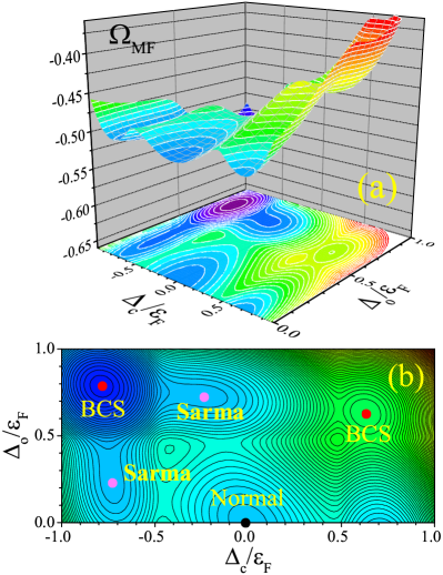
Figure 1: (color online). The landscape of thermodynamic potential (in units of $N\varepsilon_{F}$) in the $\Delta_{c}-\Delta_{o}$ plane, in a three-dimensional plot (a) or in a contour plot (b). Here, we take $1/k_{F}a_{s0}=-0.5$ and $1/k_{F}a_{s1}=-0.05$, $\mu=0.6\varepsilon_{F}$, $\delta(B)=0$ and $\delta\mu=0.5\varepsilon_{F}$. In the contour plot, the different competing phases corresponding to the local minima are indicated. The two channels are symmetric due to zero detuning. In (b), the in-phase BCS phase, where the two order parameters have the same sign, is an excited state with an energy much higher than other local minima. We note that, the FFLO pairing is not allowed with this set of interaction parameters (i.e., too strong inter-band coupling).

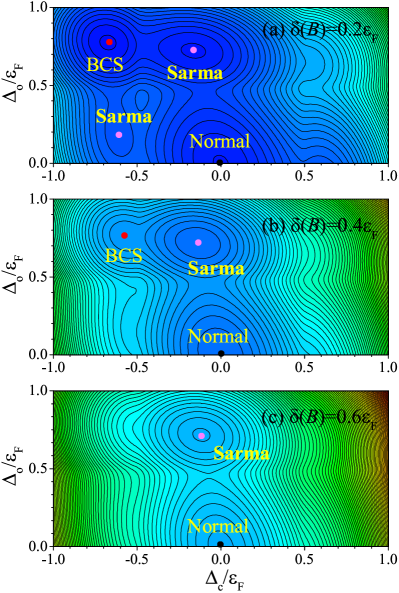
Figure 2: (color online). The contour plots of thermodynamic potential in the $\Delta_{c}-\Delta_{o}$ plane, with increasing detuning: (a) $\delta(B)=0.2\varepsilon_{F}$, (b) $\delta(B)=0.4\varepsilon_{F}$, and (c) $\delta(B)=0.6\varepsilon_{F}$. The color shows the magnitude of the thermodynamic potential $\Omega_{\textrm{MF}}$, from blue (small $\Omega_{\textrm{MF}}$) to red (large $\Omega_{\textrm{MF}}$). Various stable phases (i.e., local minima) are indicated. As the detuning increases, the pairing type in the closed channel changes from the BCS to the Sarma pairing. Here, we take $1/k_{F}a_{s0}=-0.5$ and $1/k_{F}a_{s1}=-0.05$, $\mu=0.6\varepsilon_{F}$ and $\delta\mu=0.5\varepsilon_{F}$.

III.1 Sarma pairing at a strong inter-channel coupling

Figure 1 reports various candidate phases of an imbalance superfluid near OFR with a chemical potential difference $\delta\mu=0.5\varepsilon_{F}$, in the landscape of the thermodynamic potential. These candidate states correspond to the local minima in the landscape. Here, we take a strong inter-channel coupling $1/k_{F}a_{s1}=-0.05$, at which the FFLO pairing seems to be unfavorable, and work with a grand canonical ensemble, where the chemical potential is fixed to $\mu=0.6\varepsilon_{F}$. We also consider a zero detuning $\delta(B)=0$ so that the two channels are actually symmetric against each other.

It is readily seen that a nonzero chemical potential difference $\delta\mu\neq 0$ gives the possibility of Sarma pairing in the open or closed channel, as indicated in Fig. 1(b). The two Sarma phases, which can be labelled as [BCS]_o[Sarma]_c (i.e., $\left|\Delta_{o}\right|>\delta\mu$ and $\left|\Delta_{c}\right|<\delta\mu$) and [Sarma]_o[BCS]_c ($\left|\Delta_{o}\right|<\delta\mu$ and $\left|\Delta_{c}\right|>\delta\mu$) respectively, should be understood as the same state, due to the equivalence of the two channels at zero detuning. They are more energetically favorable than the normal state with vanishing order parameters $\Delta_{o}=\Delta_{c}=0$. However, they are two local minima only in the landscape of thermodynamic potential. The global minimum is given by a BCS phase with both order parameters larger than the chemical potential difference, $\left|\Delta_{o}\right|=\left|\Delta_{c}\right|>\delta\mu$.

The situation dramatically changes when we tune the detuning by switching on an external Zeeman field. As shown in Fig. 2, with increasing detuning, the energy of the BCS phase and of one of the Sarma phase [Sarma]_o[BCS]_c increases, and both of them disappear at sufficiently large detuning. In contrast, the Sarma phase [BCS]_o[Sarma]_c decreases its energy and becomes the global minimum at about $\delta(B)\simeq 0.4\varepsilon_{F}$. Therefore, we find an energetically stable Sarma phase as the absolute ground state.

Our finding is consistent with the previous observation that the Sarma phase can be stabilized by introducing an asymmetry between the two channels or bands He2009 . However, there is an important difference. The asymmetry between the two channels in the previous work is caused by the different intra-channel interaction strengths. In our case, the intra-channel coupling is always the same. The asymmetry of the two channels is induced by engineering the single-particle behavior, i.e., changing the detuning in the closed channel.

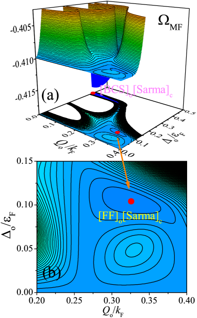
Figure 3: (color online). The landscape of thermodynamic potential (in units of $N\varepsilon_{F}$) in the $Q_{o}-\Delta_{o}$ plane, in a three-dimensional plot (a) or in a zoom-in contour plot to better view the extremely shallow FF solution (b). Here, we use $1/k_{F}a_{s0}=-0.5$ and $1/k_{F}a_{s1}=-5.0$, $\mu=0.8\varepsilon_{F}$, $\delta(B)=0.4\varepsilon_{F}$, and $\delta\mu=0.235\varepsilon_{F}$.

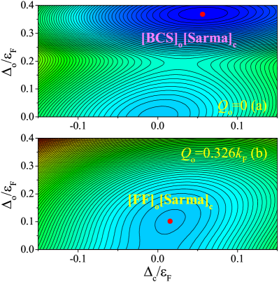
Figure 4: (color online). The landscape of thermodynamic potential in the $\Delta_{c}-\Delta_{o}$ plane, with (a) $Q_{o}=0$ and (b) $Q_{o}\simeq 0.326k_{F}$.

III.2 Fulde-Ferrell pairing at a weak inter-channel coupling

To fully establish the thermodynamic stability of the Sarma phase in our two-channel model, it is necessary to examine its instability against the formation of a FFLO superfluid. The latter is often energetically favorable at large spin-population imbalance in the weak-coupling limit Fulde1964 ; Larkin1964 . To this aim, we choose a weak inter-channel coupling with $1/k_{F}a_{s1}=-5.0$ and increase slightly the chemical potential to $\mu=0.8\varepsilon_{F}$. We fix the detuning to $\delta(B)=0.4\varepsilon_{F}$ and tune the chemical potential difference $\delta\mu$ to search for the existence of a FF superfluid.

It turns out that the FF pairing in the open channel occurs in a very narrow interval of the chemical potential difference. In Fig. 3, we present an example at $\delta\mu=0.235\varepsilon_{F}$. The landscape of thermodynamic potential is shown as functions of the open-channel order parameter $\Delta_{o}$ and the FF momentum $Q_{o}$. For a given set of $\Delta_{o}$ and $Q_{o}$, we have used the gap equation $\Delta_{c}=\Delta_{o}F_{o}(\Delta_{o},Q_{o})/\lambda_{1}$ to determine the pairing order parameter in the closed channel. It can be seen from the landscape that a very shallow FF minimum appears at about $Q_{o}\simeq 0.326k_{F}$. To confirm the FF phase is indeed a local minimum of $\Omega_{\textrm{MF}}(\Delta_{o},\Delta_{c};Q_{o},Q_{c}=0)$, in Fig. 4(b) we have further checked the contour plot of thermodynamic potential in the plane of $\Delta_{c}$ and $\Delta_{o}$, at the optimal momentum of the FF solution $Q_{o}\simeq 0.326k_{F}$. We find that the FF pairing in the open channel is accompanied with a Sarma pairing in the closed channel, since $\left|\Delta_{c}\right|\ll\delta\mu=0.235\varepsilon_{F}$. Thus, we denote the FF phase as [FF]_o[Sarma]_c. For comparison, we also show in Fig. 4(a) the contour plot of thermodynamic potential at $Q_{o}=0$. It is clear that, at the chosen parameters, the Sarma phase [BCS]_o[Sarma]_c has a much lower energy than the FF phase [FF]_o[Sarma]_c.

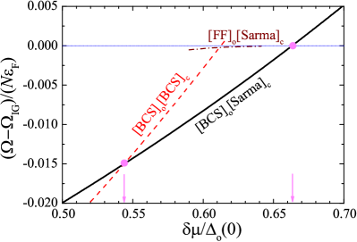
Figure 5: (color online). Thermodynamic potentials of different completing phases, in relative to the ideal Fermi gas result $\Omega_{IG}$ and in units of $N\varepsilon_{F}$, as a function of the chemical potential difference $\delta\mu$. The two arrows indicate the positions of the two phase transitions at $\delta\mu_{c1}\simeq 0.543\Delta_{o}(0)$ and $\delta\mu_{c2}\simeq 0.662\Delta_{o}(0)$, respectively. Here, we take $1/k_{F}a_{s0}=-0.5$ and $1/k_{F}a_{s1}=-5.0$, $\mu=0.8\varepsilon_{F}$, and $\delta(B)=0.4\varepsilon_{F}$. At $\delta\mu=0$, the pairing gap in the open channel of the low-energy out-of-phase solution is $\Delta_{o}(0)=0.3898\varepsilon_{F}$.

III.3 Phase diagram at the weak inter-channel coupling

By tuning the chemical potential difference $\delta\mu$, we determine the phase diagram at the given chemical potential $\mu=0.8\varepsilon_{F}$ and at the weak inter-channel coupling, as reported in Fig. 5. It can be easily seen that, the [FF]_o[Sarma]_c phase is always not energetically favorable, compared with the [BCS]_o[Sarma]_c phase. With increasing $\delta\mu$, the imbalanced Fermi gas changes from the BCS phase ([BCS]_o[BCS]_c) to the [BCS]_o[Sarma]_c phase, and finally becomes normal. All the transitions are first-order phase transition.

Therefore, we conclude that a superfluid with the FF pairing form is not supportive in the two-channel system in three dimensions. Actually, there is already some indications of this tendency, even if we do not consider the possibility of the [BCS]_o[Sarma]_c phase. In the weakly interacting single-channel case, it is well-known theoretically that a three-dimensional FF superfluid may exist in the window $0.707\Delta(0)<\delta\mu<0.754\Delta(0)$ He2006 ; Casalbuoni2004 . In our two-channel case, the inter-channel coupling changes the BCS pairing in the closed channel to the Sarma pairing and also modifies the window to $0.612\Delta_{o}(0)<\delta\mu<0.641\Delta_{o}(0)$, which is narrower than the single-channel case.

It is worth noting that for the FFLO superfluid, we may also consider the LO pairing, which is known to have a lower energy than the FF pairing. However, in the vicinity of the transition from FFLO to a normal state, both LO and FF superfluid have very similar energy and the critical chemical potential difference at the transition will not change Casalbuoni2004 , if we use a more accurate LO pairing order parameter. The only possible change is that, with increasing $\delta\mu$, we may have a transition from the BCS phase to [LO]_o[Sarma]_c, and then to [BCS]_o[Sarma]_c. This seems unlikely to happen.

The situation may qualitatively change if we focus on a low-dimensional system, where the phase space for FFLO becomes larger Hu2007 ; Liu2007 ; Orso2007 ; Toniolo2017 . In that case, intuitively the energy of the [FF]_o[Sarma]_c phase may become lower than that of the [BCS]_o[Sarma]_c phase near the superfluid-normal transition. The sequence of phase transitions is then, [BCS]_o[BCS]_c $\rightarrow$ [BCS]_o[Sarma]_c $\rightarrow$ [FFLO]_o[Sarma]_c $\rightarrow$ normal, with increasing chemical potential difference. More interestingly, the FFLO pairing may occur in both channels, leading to the phase [FFLO-$Q_{1}$]_o[FFLO-$Q_{2}$]_c, where the FFLO momenta $Q_{1}$ and $Q_{2}$ in the two channels can be the same or different, depending on the channel coupling. The resultant rich and complex phase diagram in one-dimension has been recently explored by Machida and co-workers Mizushima2013 ; Takahashi2014 , considering a Pauli-limiting two-band superconductor.

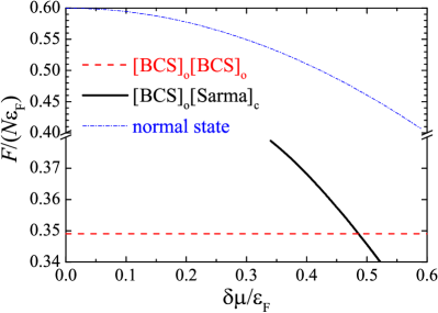
Figure 6: (color online). Free energies of different completing phases (in units of $N\varepsilon_{F}$) as a function of the chemical potential difference $\delta\mu$, at a fixed total density $\rho=3\pi^{2}k_{F}^{3}$. The [BCS]_o[Sarma]_c state becomes favorable above the threshold $\delta\mu_{c}\simeq 0.486\varepsilon_{F}$. Here, we use $1/k_{F}a_{s0}=-0.5$ and $1/k_{F}a_{s1}=-0.05$, and $\delta(B)=0.4\varepsilon_{F}$.

III.4 Phase diagram of free energy with varying chemical potential difference

We now consider the phase diagram at a fixed total number density $\rho$ and focus on the case of the strong inter-channel coupling with $1/k_{F}a_{s1}=-0.05$, in which the FF phase is absent. In Fig. 6, we report the free energy $F=\Omega+\mu\rho$ of the three competing phases. In this canonical ensemble for the chosen parameters, the [BCS]_o[Sarma]_c appears at $\delta\mu\simeq 0.3\varepsilon_{F}$, becomes energetically favorable at $\delta\mu\simeq 0.486\varepsilon_{F}$, and finally disappears at about $\delta\mu\simeq 0.53\varepsilon_{F}$, with a vanishingly small $\Delta_{c}$. At a large chemical potential difference $\delta\mu>0.53\varepsilon_{F}$, we thus expect a phase-separation phase in real space Bedaque2003 , consisting of both [BCS]_o[BCS]_c and the normal state.

IV Collective modes of a Sarma superfluid

Ideally, a Sarma superfluid may be experimentally detected by measuring the momentum distribution $\rho(\mathbf{k})$ after time-of-flight expansion Yi2006 or by measuring the momentum-resolved radio-frequency spectroscopy that gives directly the single-particle spectral function $\mathcal{A}(\mathbf{k},\omega)$ Stewart2008 . These probes cannot be universally applied to all fermionic species of ultracold atoms. For example, for ⁶Li atoms near a broad Feshbach resonance, the strong inter-particle interactions will qualitatively change the momentum distribution during the early stage of time-of-flight. These measurements are possible only for atomic species that has a relatively narrow Feshbach resonance, such as ⁴⁰K, in which one can quickly switch the magnetic field to the non-interacting limit, to avoid the convert of the interaction energy to the kinetic energy during the expansion.

A universal theme to probe a strongly interacting Sarma superfluid is provided by Bragg spectroscopy, which measures the density-density dynamic structure factor and determines low-energy collective excitations of the system Lingham2014 . In this section, we discuss the collective modes of BCS and Sarma phases and show that a Sarma superfluid in the form of [BCS]_o[Sarma]_c has some unique features in its collective excitations, as a consequence of the fact $\left|\Delta_{c}\right|<\delta\mu$.

Theoretically, the basic information of low-energy collective modes, such as the mode frequency and the damping rate, can be extracted from the vertex function, which can be regarded as the Green function of Cooper pairs in the lowest-order approximation He2016 ; Hu2006EPL ; Diener2008 . To obtain the vertex function, we expand the effective action around the mean-field saddle point and the resultant Gaussian fluctuation part $\mathcal{S}_{\textrm{GF}}$ is given by,

$$\mathcal{S}_{\textrm{GF}}=\frac{1}{2}\sum_{Q}\left[\phi_{o}^{*}\left(Q\right),\phi_{o}\left(-Q\right),\phi_{c}^{*}\left(Q\right),\phi_{c}\left(-Q\right)\right]\left[-\Gamma^{-1}\left(Q\right)\right]\left[\phi_{o}\left(Q\right),\phi_{o}^{*}\left(-Q\right),\phi_{c}\left(Q\right),\phi_{c}^{*}\left(-Q\right)\right]^{T}$$ (35)

where $Q\equiv(\mathbf{q},i\nu_{l})$ and $i\nu_{l}=i2\pi lk_{B}T$ ($l=0,\pm 1,\pm 2,\cdots$) are the bosonic Matsubara frequencies, and the inverse vertex function is He2016

$$-\Gamma^{-1}\left(\mathbf{q},i\nu_{l}\right)\equiv\left[\begin{array}[]{cccc}-\lambda_{0}+M_{11}^{(o)}&M_{12}^{(o)}&-\lambda_{1}&0\\ M_{21}^{(o)}&-\lambda_{0}+M_{22}^{(o)}&0&-\lambda_{1}\\ -\lambda_{1}&0&-\lambda_{0}+M_{11}^{(c)}&M_{12}^{(c)}\\ 0&-\lambda_{1}&M_{21}^{(c)}&-\lambda_{0}+M_{22}^{(c)}\end{array}\right]=-\left[\begin{array}[]{cc}\Gamma_{(o)}^{-1}\left(\mathbf{q},i\nu_{l}\right)&\textrm{diag}\{\lambda_{1},\lambda_{1}\}\\ \textrm{diag}\{\lambda_{1},\lambda_{1}\}&\Gamma_{(c)}^{-1}\left(\mathbf{q},i\nu_{l}\right)\end{array}\right]$$ (36)

with the matrix elements at zero temperature ($n=o,c$),

$$M_{11}^{(n)} = \sum_{\mathbf{k}}\left[v_{n-}^{2}u_{n+}^{2}\frac{f_{n-}-f_{n+}}{i\nu_{l}+E_{n-}-E_{n+}}+u_{n-}^{2}u_{n+}^{2}\frac{1-f_{n+}}{i\nu_{l}-E_{n-}-E_{n+}}-v_{n-}^{2}v_{n+}^{2}\frac{1-f_{n-}}{i\nu_{l}+E_{n-}+E_{n+}}+\frac{M}{\hbar^{2}\mathbf{k}^{2}}\right],$$ (37)

$$M_{12}^{(n)} = \sum_{\mathbf{k}}\left(uv\right)_{n-}\left(uv\right)_{n+}\left[\frac{f_{n-}-f_{n+}}{i\nu_{l}+E_{n-}-E_{n+}}-\frac{1-f_{n+}}{i\nu_{l}-E_{n-}-E_{n+}}+\frac{1-f_{n-}}{i\nu_{l}+E_{n-}+E_{n+}}\right],$$ (38)

and $M_{21}^{(n)}(Q)=M_{12}^{(n)}(Q)$, and $M_{22}^{(n)}(Q)=M_{11}^{(n)}(-Q)$. Here, we have defined some short-hand notations,

$$E_{n\pm} \equiv E_{n\mathbf{k}\pm\mathbf{q}/2},$$ (39)

$$f_{n\pm} \equiv f\left[E_{n\mathbf{k}\pm\mathbf{q}/2}-\delta\mu\right],$$ (40)

$$u_{n\pm}^{2} = \frac{1}{2}\left(1+\frac{\xi_{n\pm}}{E_{n\pm}}\right),$$ (41)

$$v_{n\pm}^{2} = \frac{1}{2}\left(1-\frac{\xi_{n\pm}}{E_{n\pm}}\right),$$ (42)

$$\left(uv\right)_{n\pm} = \frac{1}{2}\frac{\Delta_{n}}{E_{n\pm}}.$$ (43)

The low-lying collective excitation spectrum is determined by the pole of $\Gamma(\mathbf{q},i\nu_{l}\rightarrow\omega+i0^{+})$ after analytic continuation He2016 ; Zhang2017 ; Matera2017 .

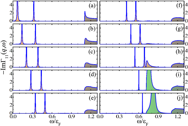
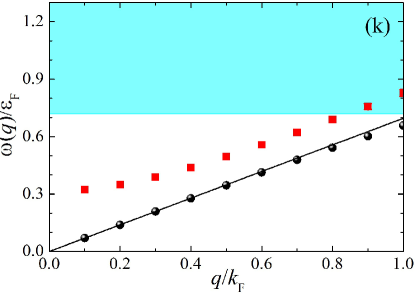
Figure 7: (color online). (a)-(j) The spectral function of Cooper pairs $-\textrm{Im}\Gamma_{11}(q,\omega)$ at different transferred momenta, which increase from $0.1k_{F}$ to $1.0k_{F}$ with a step $0.1k_{F}$. Here, we consider a balanced BCS state with a fixed total density $\rho=3\pi^{2}k_{F}^{3}$ and $\delta\mu=0$. The detuning is $\delta(B)=0.4\varepsilon_{F}$. (k) The dispersion relation of the phonon (black circles) and Leggett modes (red squares). The shaded area in cyan color shows the two-particle excitation continuum. The error bar in red squares in the two-particle continuum indicates the damping width of the peak, due to the coupling to fermionic quasiparticles. The straight line shows $\omega=c_{s}q$, where $c_{s}\simeq 0.348v_{F}$ is the sound velocity.

It is clear from Eq. (36) that the total vertex function is constructed from the two vertex functions in each channel coupled by the inter-channel coupling matrix $\textrm{diag}\{\lambda_{1},\lambda_{1}\}$, which is diagonal. In the absence of coupling, it is well-known that each vertex function supports a gapless Goldstone-Anderson-Bogoliubov phonon mode, due to phase fluctuations of the pairing order parameter. As we shall see He2016 ; Zhang2017 , with inter-channel coupling, one gapless mode remains, corresponding to the in-phase phase fluctuations of the two order parameters. It is ensured by the condition

$$\det\Gamma^{-1}\left(\mathbf{q}=0,i\nu_{l}=0\right)=0,$$ (44)

which is exactly equivalent to the gap equations Eq. (30) and Eq. (31). The other gapless mode, corresponding to the out-of-phase phase fluctuations, is lifted to have a finite energy in the low-wavelength limit. This is the so-called massive Leggett mode Leggett1966 , which is not observed with cold-atoms yet.

From the expressions Eq. (37) and Eq. (38) of the matrix elements $M_{11}^{(n)}$ and $M_{12}^{(n)}$, one may easily identify that collective excitations are coupled to the two types of single-particle excitations: (i) pair-breaking excitations, in which two Bogoliubov quasi-particles are created or annihilated with possibility $u_{n-}^{2}u_{n+}^{2}(1-f_{n+})$ or $v_{n-}^{2}v_{n+}^{2}(1-f_{n-})$. These are given in the second and third terms of the matrix elements; and (ii) particle-hole excitations, in which one Bogoliubov quasi-particle is scattered into another quasi-particle state, with possibility proportional to the number of quasi-particles present, i.e., $f_{n-}-f_{n+}$. This process is described by the first term of the matrix elements.

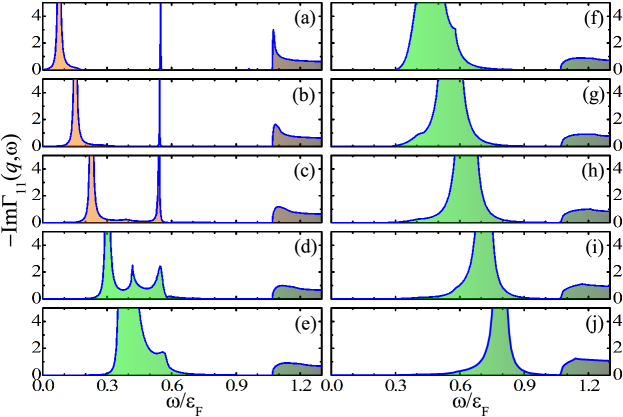
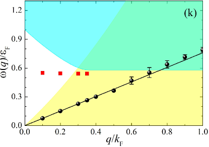
Figure 8: (color online). (a)-(j) The spectral function of Cooper pairs $-\textrm{Im}\Gamma_{11}(q,\omega)$ at different transferred momenta, which increase from $0.1k_{F}$ to $1.0k_{F}$ with a step $0.1k_{F}$. Here, we take the parameters $\delta(B)=0.4\varepsilon_{F}$ and $\delta\mu=0.5\varepsilon_{F}$ and consider the case of a fixed total density $\rho=3\pi^{2}k_{F}^{3}$, which lead to a Sarma state in the closed channel with $\mu_{c}=\mu-\delta(B)/2\simeq 0.25\varepsilon_{F}$ and $\Delta_{c}\simeq-0.08\varepsilon_{F}$. (k) The dispersion relation of the phonon (black circles) and Leggett modes (red squares). The shaded areas in cyan and yellow colors correspond to the two-particle (Eq. (48)) and particle-hole excitation continua (Eq. (50)), respectively. The error bar in symbols indicates the full width at half maximum of the peak in the spectral function. As the momentum increases, the Leggett peak shrinks gradually and disappears at $q\sim 0.4k_{F}$. The straight line shows $\omega=c_{s}q$, where $c_{s}\simeq 0.380v_{F}$ is the sound velocity.

IV.1 Collective modes of a BCS superfluid

In Fig. 7, we report the spectral function of Cooper pairs - the imaginary part of the 11-component of the vertex function $-\textrm{Im}\Gamma_{11}(q,\omega)$ - of a BCS superfluid, at different transferred momenta from $q=0.1k_{F}$ to $q=k_{F}$, with a step $\Delta q=0.1k_{F}$. Here, we choose the same interaction parameters as in the phase diagram Fig. 6 and set the chemical potential difference $\delta\mu=0$. The self-consistent solution of the mean-field equations at a fixed number of atoms $\rho$ leads to, $\mu_{o}\simeq 0.43\varepsilon_{F}$, $\mu_{c}\simeq 0.23\varepsilon_{F}$, $\Delta_{o}\simeq 0.55\varepsilon_{F}$ and $\Delta_{c}\simeq-0.36\varepsilon_{F}$.

For a BCS superfluid, it is clear that the particle-hole excitations are absent at zero temperature, as a result of the gapped single-particle spectrum and that all the fermionic distribution functions $f_{n\pm}$ should vanish identically. Pair-breaking excitations are possible if the frequency $\omega$ is larger than the two-particle threshold, which for the channel $n=o,c$ is given by Combescot2006 ,

$$\omega_{\textrm{2p}}^{(n)}=\left\{\begin{array}[]{cc}2\sqrt{\left(\frac{\hbar^{2}q^{2}}{8M}-\mu_{n}\right)^{2}+\Delta_{n}^{2}}&\textrm{if }\mu_{n}<\frac{\hbar^{2}q^{2}}{8M}\\ 2\left|\Delta_{n}\right|&\textrm{otherwise}\end{array}\right..$$ (45)

For small $q$, we thus obtain $\omega_{\textrm{2p}}^{(o)}=2\Delta_{o}\simeq 1.10\varepsilon_{F}$ and $\omega_{\textrm{2p}}^{(c)}=2\left|\Delta_{c}\right|\simeq 0.72\varepsilon_{F}$.

From the spectral functions at $q\leq 0.8k_{F}$, i.e., in Figs. 7(a)-7(h), one can clearly identify the gapless Goldstone-Anderson-Bogoliubov phonon mode and the massive Leggett mode, both of which are undamped, since they do not touch the two-particle continuum of either channel. For the cases with $q=0.9k_{F}$ in Fig. 7(i) and with $q=k_{F}$ in Fig. 7(j), the phonon mode remains undamped, while the Leggett mode has a frequency larger than $\omega_{\textrm{2p}}^{(c)}$ and gets damped due to the coupling to the pair-breaking excitations. The dispersion relations of the phonon mode and the Leggett mode in the BCS superfluid are summarized in Fig. 7(k).

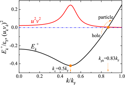
Figure 9: (color online). The dispersion relation $E_{c\mathbf{k},+}=\sqrt{\xi_{c\mathbf{k}}^{2}+\Delta_{c}^{2}}-\delta\mu$ of the lower branch of fermionic quasiparticles in the closed channel (black curve) and the square of the coherence factor $(u_{c\mathbf{k}}v_{c\mathbf{k}})^{2}$ (red curve). Here, we take the parameters $\delta(B)=0.4\varepsilon_{F}$ and $\delta\mu=0.5\varepsilon_{F}$ and consider the case of a fixed total density $\rho=3\pi^{2}k_{F}^{3}$, which lead to a Sarma state in the closed channel with $\mu_{c}=\mu-\delta(B)/2\simeq 0.25\varepsilon_{F}$ and $\Delta_{c}\simeq-0.08\varepsilon_{F}$. The dispersion relation has gapless particle-hole excitations near the wavevectors $\left|\mathbf{k}\right|=k_{\mathbf{\textrm{ph}}}\simeq 0.83k_{F}$. The factor $(u_{c\mathbf{k}}v_{c\mathbf{k}})^{2}$ peaks near the minimum of the dispersion relation ($k_{c}\simeq 0.5k_{F}$).

IV.2 Collective modes of a Sarma superfluid

The collective modes of a Sarma superfluid are quite different, because of the gapless single-particle excitations. In Fig. 8, we present the spectral function $-\textrm{Im}\Gamma_{11}(q,\omega)$ of a Sarma superfluid, as the transferred momentum evolves from $q=0.1k_{F}$ to $q=k_{F}$ in step of $\Delta q=0.1k_{F}$. To have a Sarma phase in the closed channel, we again choose the interaction parameters as in Fig. 6 and take the chemical potential difference $\delta\mu=0.5\varepsilon_{F}$. The mean-field solution at the fixed density $\rho$ gives $\mu_{o}\simeq 0.45\varepsilon_{F}$, $\mu_{c}\simeq 0.25\varepsilon_{F}$, $\Delta_{o}\simeq 0.54\varepsilon$ and $\Delta_{c}\simeq-0.08\varepsilon_{F}$. For the lower branch of fermionic quasiparticles in the closed channel, we show its dispersion relation $E_{c\mathbf{k},+}=\sqrt{\xi_{c\mathbf{k}}^{2}+\Delta_{c}^{2}}-\delta\mu$ in Fig. 9. The closed-channel dispersion relation has a node at $k_{\textrm{ph}}\simeq 0.83k_{F}$ and has a minimum at $k_{c}\simeq 0.5k_{F}$.

At the smallest $q$ considered, as shown in Fig. 8(a), we find the anticipated phonon mode and Leggett mode, as in the case of a BCS superfluid. As $q$ increases, however, the situation becomes different. While the phonon mode remains well-defined, the massive Leggett mode gradually loses its weight and finally disappears at $q\sim 0.4k_{F}$. By further increasing $q$, a damped phonon mode with nonzero damping width is observed, up to the largest transferred momentum considered in the figure (i.e., $q=k_{F}$). The dispersion relations of the phonon mode and the Leggett mode in the Sarma superfluid are summarized in Fig. 8(k).

The vanishing Leggett mode and the damped phonon mode at $q\apprge 0.4k_{F}$ may be understood from the gapless single-particle spectrum, which allows nonzero fermionic distribution functions $f_{n\pm}>0$ and hence the gapless particle-hole excitations. As discussed in Appendix B, the collective modes couple to the particle-hole excitations if their frequency $\omega$ is within the particle-hole continuum, i.e.,

$$0<\omega<\omega_{\textrm{ph}}=\sqrt{\left[\frac{\hbar^{2}(k_{\textrm{ph}}+q)^{2}}{2m}-\mu_{c}\right]+\Delta_{c}^{2}}-\delta\mu.$$ (46)

This particle-hole continuum has been indicated in Fig. 8(k) in yellow. We find that the Leggett mode is fragile towards the excitations of particle-hole pairs. The phonon mode seems to be more robust. In particular, the damping rate of the phonon mode due to the coupling to the particle-hole excitations can hardly be noticed at $q\lesssim 0.3k_{F}$, because of the small coherence factors (see Appendix B for more details).

On the other hand, it is somehow surprising to find a well-defined, undamped Leggett mode at $q\sim 0$. Naïvely, one may think that the two-particle threshold for the closed channel is $\omega_{\textrm{2p}}^{(c)}=2\left|\Delta_{c}\right|\simeq 0.16\varepsilon_{F}$. As the frequency of the Leggett mode is about $\omega\sim 0.6\varepsilon_{F}>\omega_{\textrm{2p}}^{(c)}$, it should be damped by the process of breaking a Cooper pair. This is not correct, as the two-particle threshold completely changes in the Sarma phase, again due to the nonzero fermionic distribution functions $f_{n\pm}>0$. As discussed in Appendix A, at $q\sim 0$ the two-particle threshold $\omega_{\textrm{2p}}^{(c)}$ should be about $2\delta\mu=\varepsilon_{F}$, much larger than the naïve result of $2\left|\Delta_{c}\right|\simeq 0.16\varepsilon_{F}$. The large two-particle threshold, as shown in Fig. 8(k) in cyan, ensures an undamped Leggett mode at low transferred momentum.

V Conclusions

In summary, we have theoretically investigated the imbalanced superfluidity of a three-dimensional strongly interacting Fermi gas near orbital Feshbach resonances. The system can be well treated as a specific realization of the two-band or two-channel model He2015TwoBandTheory , with symmetric intra-channel inter-particle interactions. We have found that by engineering the detuning (i.e., chemical potential) of the closed channel via an external magnetic field, the induced asymmetry in the single-particle dispersion relation between open and closed channels can thermodynamically stabilize a Sarma pairing in the closed channel. In three dimensions, we have predicted that the resultant Sarma superfluid is robust against the formation of a spatially inhomogeneous Fulde–Ferrell–Larkin–Ovchinnikov superfluid in the large spin-polarization limit.

As a consequence of the gapless fermionic quasi-particle excitations, the Sarma superfluid has a damped Goldstone-Anderson-Bogoliubov phonon mode even at zero temperature. The damping rate of the phonon mode becomes significant at moderate transferred momentum. The Sarma superfluid also has a well-defined, undamped massive Leggett mode at low momentum, due to the lifted two-particle continuum. However, as the transferred momentum increases, the Leggett mode disappears once it enters the particle-hole continuum. Experimentally, these peculiar features of the collective modes of the Sarma superfluid can be measured by using Bragg spectroscopy.

In one dimension or two dimensions, the Fulde–Ferrell–Larkin–Ovchinnikov superfluidity may become favorable due to the reduced dimensionality Hu2007 ; Liu2007 ; Orso2007 ; Toniolo2017 . In that cases, we anticipate a rich and complicated phase diagram Mizushima2013 ; Takahashi2014 . Moreover, it is interesting to understand the pair fluctuations in a strongly interacting Sarma superfluid, based on the standard Gaussian pair fluctuation theory Hu2006EPL ; Diener2008 or the functional renormalization group Boettcher2015PLB ; Strack2014 ; Boettcher2015PRA . These possibilities will be explored in future studies.

Appendix A The two-particle continuum of a Sarma superfluid

In this appendix, we consider a Sarma superfluid with dispersion relations $E_{\mathbf{k},+}=E_{\mathbf{k}}-\delta\mu$ (lower branch) and $E_{\mathbf{k},-}=E_{\mathbf{k}}+\delta\mu$ (upper branch), where $E_{\mathbf{k}}=\sqrt{\xi_{\mathbf{k}}^{2}+\Delta^{2}}$. We aim to calculate the two-particle threshold of the Sarma superfluid,

$$\omega_{\textrm{2p}}\left(\mathbf{q}\right)=\min_{\{\mathbf{k}\}}\left[E_{\mathbf{k}}+E_{\mathbf{k}+\mathbf{q}}\right],$$ (47)

under the condition that $E_{\mathbf{k}}\geq\delta\mu$ (see the second and third terms in Eq. (37) and Eq. (38), contributed from the two-particle excitations). At zero momentum $\mathbf{q}=0$, we find immediately that $\omega_{\textrm{2p}}=2\delta\mu$. For nonzero momentum $q$, let us assume that the single-particle dispersion relation has a minimum at $k_{c}=\sqrt{2m\mu}/\hbar$ ($\mu>0$) and has a zero at $k_{\textrm{ph}}=[2m(\mu+\sqrt{\delta\mu^{2}-\Delta^{2}})]^{1/2}/\hbar$ (see Fig. 9). Using $E_{\mathbf{k}+\mathbf{q}}=\sqrt{[\hbar^{2}(\mathbf{k}+\mathbf{q})^{2}/2m-\mu]^{2}+\Delta^{2}}$, it is easy to obtain that,

$$\omega_{\textrm{2p}}=\left\{\begin{array}[]{cc}\delta\mu+\sqrt{\left[\frac{\hbar^{2}(k_{\textrm{ph}}-q)^{2}}{2m}-\mu\right]+\Delta^{2}},&q<k_{\textrm{ph}}-k_{c}\\ \delta\mu+\left|\Delta\right|,&\left|q-k_{\textrm{ph}}\right|\leq+k_{c}\\ \delta\mu+\sqrt{\left[\frac{\hbar^{2}(k_{\textrm{ph}}-q)^{2}}{2m}-\mu\right]+\Delta^{2}}.&k_{\textrm{ph}}+k_{c}<q\end{array}\right.$$ (48)

Appendix B The particle-hole continuum of a Sarma superfluid

We now turn to consider the particle-hole continuum. We want to determine,

$$\omega_{\textrm{ph}}\left(\mathbf{q}\right)=\max_{\{\mathbf{k}\}}\left[E_{\mathbf{k}+\mathbf{q}/2}-E_{\mathbf{k}-\mathbf{q}/2}\right],$$ (49)

under the constraints $E_{\mathbf{k}+\mathbf{q}/2}>\delta\mu>E_{\mathbf{k}-\mathbf{q}/2}$ (see the first term in Eq. (37) and Eq. (38)). The collective mode couples to the particle-hole excitations and is damped, if its frequency $0<\omega<\omega_{\textrm{ph}}$. These particle-hole excitations occur at around $k_{\textrm{ph}}$. It is readily seen that in order to reach the maximum, we must have $\mathbf{k}\parallel\mathbf{q}$ and $k=k_{\textrm{ph}}+q/2$. This leads to,

$$\omega_{\textrm{ph}}=\sqrt{\left[\frac{\hbar^{2}(k_{\textrm{ph}}+q)^{2}}{2m}-\mu\right]+\Delta^{2}}-\delta\mu.$$ (50)

It is worth noting that when $0<\omega<\omega_{\textrm{ph}}$ the damping of the collective mode due to the particle-hole excitations depends on the coherent factor $u_{\mathbf{k}\pm\mathbf{q}/2}v_{\mathbf{k}\pm\mathbf{q}/2}$ (see the first term in Eq. (37) and Eq. (38) for the matrix elements $M_{11}$ and $M_{12}$). The coherence factor is significant at about $k_{c}$ only, as shown in Fig. 9, which implies a resonant condition $k_{\textrm{ph}}-q/2\sim k_{c}$. This means that the damping due to particle-hole excitations becomes important at $q\sim 2(k_{\textrm{ph}}-k_{c})$.

References

- (1) G. Sarma, J. Phys. Chem. Solids 24, 1029 (1963).
- (2) W. V. Liu and F. Wilczek, Phys. Rev. Lett. 90, 047002 (2003).
- (3) S.-T. Wu and S. Yip, Phys. Rev. A 67, 053603 (2003).
- (4) M. M. Forbes, E. Gubankova, W. V. Liu, and F. Wilczek, Phys. Rev. Lett. 94, 017001 (2005).
- (5) L. Radzihovsky and D. E. Sheehy, Rep. Prog. Phys. 73, 076501 (2010).
- (6) F. Chevy and C. Mora, Rep. Prog. Phys. 73, 112401 (2010).
- (7) K. B. Gubbels and H. T. C. Stoof, Phys. Rep. 525, 255 (2013).
- (8) J. J. Kinnunen, J. E. Baarsma, J.-P. Martikainen, and P. Törmä, arXiv:1706.07076.
- (9) P. F. Bedaque, H. Caldas, and G. Rupak, Phys. Rev. Lett. 91, 247002 (2003).
- (10) P. Fulde and R. A. Ferrell, Phys. Rev. 135, A550 (1964).
- (11) A. I. Larkin and Y. N. Ovchinnikov, Zh. Eksp. Teor. Fiz. 47, 1136 (1964) [Sov. Phys. JETP 20, 762 (1965)].
- (12) I. Boettcher, T. K. Herbst, J. M. Pawlowski, N. Strodthoff, L. von Smekal, and C. Wetterich, Phys. Lett. B 742, 86 (2015).
- (13) M. Zwierlein, A. Schirotzek, C. H. Schunck, and W. Ketterle, Science 311, 492 (2006).
- (14) G. B. Partridge, W. Li, R. I. Kamar, Y.-a. Liao, and R. G. Hulet, Science 311, 503 (2006).
- (15) Y. Liao, A. S. C. Rittner, T. Paprotta, W. Li, G. B. Partridge, R. G. Hulet, S. K. Baur, and E. J. Mueller, Nature (London) 467, 567 (2010).
- (16) M. M. Parish, F. M. Marchetti, A. Lamacraft, and B. D. Simons, Phys. Rev. Lett. 98, 160402 (2007).
- (17) J. E. Baarsma, K. B. Gubbels, and H. T. C. Stoof, Phys. Rev. A 82, 013624 (2010).
- (18) J. Wang, Y. Che, L. Zhang, and Q. Chen, Sci. Rep. 7, 39783 (2017).
- (19) I. Bloch, J. Dalibard, and W. Zwerger, Rev. Mod. Phys. 80, 885 (2008).
- (20) S. Giorgini, L. P. Pitaevskii, and S. Stringari, Rev. Mod. Phys. 80, 1215 (2008).
- (21) M. Randeria and E. Taylor, Annu. Rev. Condens. Matter Phys. 5, 209 (2014).
- (22) D. E. Sheehy and L. Radzihovsky, Phys. Rev. Lett. 96, 060401 (2006).
- (23) D. E. Sheehy and L. Radzihovsky, Ann. Phys. (N.Y.) 322, 1790 (2007).
- (24) H. Hu and X.-J. Liu, Phys. Rev. A 73, 051603(R) (2006).
- (25) L. He and P. Zhuang, Phys. Rev. B 79, 024511 (2009).
- (26) R. Zhang, Y. Cheng, H. Zhai, and P. Zhang, Phys. Rev. Lett. 115, 135301 (2015).
- (27) G. Pagano, M. Mancini, G. Cappellini, L. Livi, C. Sias, J. Catani, M. Inguscio, and L. Fallani, Phys. Rev. Lett. 115, 265301 (2015).
- (28) M. Höfer, L. Riegger, F. Scazza, C. Hofrichter, D. R. Fernandes, M. M. Parish, J. Levinsen, I. Bloch, and S. Fölling, Phys. Rev. Lett. 115, 265302 (2015).
- (29) L. He, J. Wang, S.-G. Peng, X.-J. Liu, and H. Hu, Phys. Rev. A 94, 043624 (2016).
- (30) L. He, X.-J. Liu, and H. Hu, Phys. Rev. A 91, 023622 (2015).
- (31) M. Iskin, Phys. Rev. A 94, 011604(R) (2016).
- (32) J. Xu, R. Zhang, Y. Cheng, P. Zhang, R. Qi, and H. Zhai, Phys. Rev. A 94, 033609 (2016).
- (33) Y.-C. Zhang, S. Ding, and S. Zhang, Phys. Rev. A 95, 041603 (2017).
- (34) M. Iskin Phys. Rev. A 95, 013618 (2017).
- (35) S. Mondal, D. Inotani, and Y. Ohashi, arXiv:1709.00154 (2017).
- (36) J.-G. Chen, T.-S. Deng, W. Yi, and W. Zhang Phys. Rev. A 94, 053627 (2016).
- (37) J. Xu and R. Qi, arXiv:1710.00785 (2017).
- (38) J.-G. Chen, Y.-R. Shi, X. Zhang, and W. Zhang, arXiv:1801.09375 (2018).
- (39) A. J. Leggett, Prog. Theor. Phys. 36, 901 (1966).
- (40) M.G. Lingham, K. Fenech, S. Hoinka, and C.J. Vale, Phys. Rev. Lett. 112, 100404 (2014).
- (41) C. A. R. Sá de Melo, M. Randeria, and J. R. Engelbrecht, Phys. Rev. Lett. 71, 3202 (1993).
- (42) H. Hu, X.-J. Liu, and P. D. Drummond, Europhys. Lett. 74, 574 (2006).
- (43) R. B. Diener, R. Sensarma, and M. Randeria, Phys. Rev. A 77, 023626 (2008).
- (44) L. He, H. Lü, G. Cao, H. Hu, and X.-J. Liu, Phys. Rev. A 92, 023620 (2015).
- (45) L. He, M. Jin, and P. Zhuang, Phys. Rev. B 73, 214527 (2006).
- (46) R. Casalbuoni and G. Nardulli, Rev. Mod. Phys. 76, 263 (2004).
- (47) H. Hu, X.-J. Liu, and P. D. Drummond, Phys. Rev. Lett. 98, 070403 (2007).
- (48) X.-J. Liu, H. Hu, and P. D. Drummond, Phys. Rev. A 76, 043605 (2007).
- (49) G. Orso, Phys. Rev. Lett. 98, 070402 (2007).
- (50) U. Toniolo, B. C. Mulkerin, X.-J. Liu, and H. Hu, Phys. Rev. A 95, 013603 (2017).
- (51) T. Mizushima, M. Takahashi, and K. Machida, J. Phys. Soc. Jpn. 83, 023703 (2013).
- (52) M. Takahashi, T. Mizushima, and K. Machida, Phys. Rev. B 89, 064505 (2014).
- (53) W. Yi and L.-M. Duan, Phys. Rev. Lett. 97, 120401(2006).
- (54) J. T. Stewart, J. P. Gaebler, and D. S. Jin, Nature (London) 454, 744 (2008).
- (55) F. Matera and M. F. Wagner, Eur. Phys. J. D 71, 293 (2017).
- (56) R. Combescot, M. Yu. Kagan, and S. Stringari, Phys. Rev. A 74, 042717 (2006).
- (57) P. Strack and P. Jakubczyk, Phys. Rev. X 4, 021012 (2014).
- (58) I. Boettcher, J. Braun, T. K. Herbst, J. M. Pawlowski, D. Roscher, and C. Wetterich, Phys. Rev. A 91, 013610 (2015).