Anisotropic fixed points in Dirac and Weyl semimetals.

Abstract

The effective low energy description of interacting Dirac and Weyl semimetals is that of massless Quantum Electrodynamics with several Lorentz breaking material parameters. We perform a renormalization group analysis of Coulomb interaction in anisotropic Dirac and Weyl semimetals and show that the anisotropy persists in the material systems at the infrared fixed point. In addition, a tilt of the fermion cones breaking inversion symmetry induces a magneto–electric term in the electrodynamics of the material whose magnitude runs to match that of the electronic tilt at the fixed point.

I Introduction

The experimental realization of Dirac and Weyl semimetals (WSM) in three dimensions (3D)BGetal14; LJetal14; Xu15; Lvetal15; Xuetal15; Yanetal17 has opened a new avenue in condensed matter physics in the post–graphene era. The attraction of these materials comes in part from the shared properties with their high energy counterparts and the fruitful in-breeding that their studies bring to both communities.

The effective low energy model of interacting WSMs is very similar to massless (zero fermion mass) Quantum Electrodynamics (QED). The breakdown of Lorentz symmetry induced by various material parameters (the separation of the Weyl nodes, the departure of the Fermi velocity from the speed of light $c$ and, eventually, the tilt of the cones) does not alter significantly the renormalization properties of the system. In particular, its most relevant feature, the infrared stable fixed point, survives in these Lorentz breaking models. Lorentz invariance violating terms (LIV) in pure QED have been extensively explored in the context of Quantum Field Theory CFJ90; CK98; KM09; JK99 where astrophysical observations put severe bounds to their presence KR11. A renormalization group (RG) analysis of all the possible LIV breaking parameters was performed in KLP02 with the finding that full Lorentz invariance (rotations and boosts) is always restored at the infrared critical point.

In the condensed matter context the main question is the stability and ultimate fate of the system in the infrared limit. Systems with a regular Fermi velocity were analyzed in P93 and shown to give rise to standard Fermi liquid. Singular Fermi surfaces in 2D were explored in the early publications GGV94; GGV99 associated to graphene. There it was shown that the Fermi velocity grows monotonically till it reaches the speed of light, a result that has been later obtained by many techniques (see a recent account with a fair list of references in TK18) and was confirmed experimentally in EGetal11; MEetal12. This result is very robust although the infrared fixed point with $v_{F}=c$ is experimentally unreachable JGV10; V11. A very complete analysis of the 2D model including short range interactions has appeared in the recent publication TLetal18.

RG phases of the 3D massless QED problem in a condensed matter framework were explored in the early works AB71; IN12 prior to the experimental realization of Dirac and Weyl semimetals (see also RJH16). The non–relativistic limit with a static Coulomb potential was later addressed in RL13; Sarma15; DFG17. A crucial difference with the 2D case is that the polarization diagram is finite in the 2D case and does not induce a renormalization of the permeability or susceptibility. The speed of light and the electric charge are not renormalized and the RG running of the effective coupling constant comes solely from the Fermi velocity renormalization. The same happens in 3D with the static Coulomb propagator. When taking into account the full retarded photon propagator in 3D the divergent polarization diagram renormalizes the velocity of light through the electric permeability and the magnetic susceptibility. The full relativistic isotropic case was analyzed in AB71; IN12; it was found that both the fermion and photon velocities run to a common, isotropic and non–universal value at the infrared fixed point. This restores Lorentz symmetry, in particular it allows to define a single Lorentz factor. Rotational invariance was not questioned in these works. The material realizations show a Fermi velocity anisotropy and tilt, both affecting the $SO(3)$ rotational symmetry, a part of the Lorentz group.

In this work we analyze the renormalization of the various parameters of the WSM interacting model using the full Coulomb interaction mediated by relativistic photons. In particular we analyze the case of an initially anisotropic dispersion relation and a tilt. Similarly to what happens in the isotropic case discussed in IN12; RJH16, we find that anisotropic fermion and photon velocities also run to a common, non–universal value at the fixed point. Hence Lorentz boosts can be defined at each particular direction but rotational symmetry is not recovered at the infrared fixed point. We also find that a tilt $t$ in the matter sector that breaks inversion symmetry ($\mathcal{I}$) induces a magneto–electric coupling in the WSM electrodynamics whose value runs to a common, non–vanishing value with $t$ in the infrared fixed point. Contrary what happens in the static limit DFG17, in this fully relativistic analysis, the tilt does not vanish in the infrared fixed point.

In contrast to the high energy context, LIVs terms of WSMs are not restricted to very small values and their experimental accessibility selects a preferred frame and allows for the anisotropic fixed point described in this work. In particular, the Fermi velocity and tilt of the interacting fermionic system can be directly observed in angle resolved photoemission (ARPES) experiments CSetal16; DWetal16; JLetal17; LWetal17, providing physical initial values for the RG flow ending in the anisotropic fixed points. Standard optical probes can also reveal birefringence associated to the time–reversal ($\mathcal{T}$) breaking tilt term.

We do not address the role of short range interactions, disorder, or non–perturbative effects leading to spontaneous symmetry breaking; some of these issues have been explored in WKA14; JG15; JG17; RGJ17; SF17. The vector $b_{\mu}$ separating the Weyl cones in $\mathcal{T}$ broken WSMs does not alter our results. Finally, the term “anisotropic WSMs" often refers to systems where the electronic dispersion around a Weyl point is linear in some directions and quadratic in others. The RG analysis is different in these cases LWL18.

II The model

Weyl fermions in WSMs can be described by a LIV extension of massless QED. Depending on the tilt of their energy cone, WSMs are classified as Type I and Type II SGetal15. The Fermi surface of Type I is a point, while Type II WSMs do have an extended Fermi surface, the electron–electron interaction is screened and the scaling analysis underlying the RG approach is substantially different (see P93) from the one of the Type I case. Hence, we focus only on type I WSMs. A dispersion relation of the form (without loss of generality we choose the tilt in the $Z$ direction)

$$E=\pm\sqrt{\sum_{i=1}^{3}v_{i}^{2}p_{i}^{2}}+tp_{3}\ ,$$ (1)

is obtained from the tree level Lagrangian

$$\mathcal{L}_{\text{F}}=i\bar{\psi}\left(\gamma^{0}\left(\partial_{0}-t\partial_{3}\right)+\sum_{i=1}^{3}\gamma^{i}v_{i}\partial_{i}\right)\psi\ ,$$ (2)

where $\psi$ is the fermionic field, $\gamma^{\mu}$ are the contravariant gamma matrices, $t$ is the tilt velocity that breaks both $\mathcal{I}$ and $\mathcal{T}$ and $v_{i}$ are the components of the Fermi velocity. In our convention the metric is $\eta_{\mu\nu}=\text{diag}\left(1,-1,-1,-1\right)$. All the velocities, including the tilt parameter, will be given in units of the speed of light in vacuum, $c_{0}=1$. The condition $|t|<|v_{3}|$ ensuring type I will be kept throughout the work.

The electromagnetic interaction is obtained by replacing the ordinary derivative of (2) by a covariant derivative

$$\mathcal{L}_{\text{int}}=-e\bar{\psi}\left(\gamma^{0}\left(A_{0}-tA_{3}\right)+\sum_{i=1}^{3}\gamma^{i}v_{i}A_{i}\right)\psi\ ,$$ (3)

where $e$ is the electric charge and $A_{\mu}$ is the photon field. Finally, we need to construct an appropriate photon propagation. The standard term in QED (in the Lorenz gauge $\partial_{\mu}A^{\mu}=0$ )

$$\mathcal{L}_{\text{ph QED}}=-\dfrac{1}{4}F_{\mu\nu}F^{\mu\nu}-\dfrac{1}{2\xi}\left(\partial_{\mu}A^{\mu}\right)^{2}\ ,$$ (4)

where $F_{\mu\nu}=\partial_{\mu}A_{\nu}-\partial_{\nu}A_{\mu}$ is the electromagnetic tensor, is too much constrained by Lorentz invariance and does not allow to renormalize the vacuum polarization divergencies arising in the anisotropic WSM. We need a term that reflects the anisotropy of the media, so we introduce a polarization tensor in which the permittivity $\epsilon$ and permeability $\mu$ (both of them will be given in units of the permittivity $\epsilon_{0}$ and permeability $\mu_{0}$ of the vacuum) depend on the direction in which they are measured.

$$\mathcal{L}_{\text{ph}}=\dfrac{1}{2}\sum_{i=1}^{3}\left(\epsilon_{i}E_{i}^{2}-\dfrac{1}{\mu_{i}}B_{i}^{2}\right)-\dfrac{1}{2\xi}\left(\partial_{\mu}A^{\mu}\right)^{2}\ ,$$ (5)

where $\vec{E}$ and $\vec{B}$ are the electric and magnetic fields defined in terms of the photon field in the standard way: $E_{i}=\partial_{0}A_{i}-\partial_{i}A_{0},\;B_{i}=-\epsilon_{ijk}\partial^{j}A^{k}.$ Finally, we will see that a fermion tilt generates additional polarization diagrams that can not be absorbed in the parameters in eq. (5). If the tilt is chosen to be in the $Z$ direction, the photon propagator needs a structure analog to the fermion tilt which consists of replacing

$$E_{1}\rightarrow E_{1}+\omega_{1}B_{2}\ ,\qquad E_{2}\rightarrow E_{2}-\omega_{2}B_{1}\ ,$$ (6)

in eq. (5) so that the permeability in the plane perpendicular to the electronic tilt is modified and a linear magneto–electric term is generated. rCl L_ph & = 12∑_i=1^3( ϵ_iE_i^2)-1μ1( 1-ω12c12 ) B_1^2
- 1μ2( 1-ω22c22 ) B_2^2- 1μ3B_3^2
+ ϵ_1ω_1E_1B_2-ϵ_2ω_2E_2B_1 -12ξ( ∂_μA^μ )^2   , where we have defined $c_{i}=c_{0}/\sqrt{\epsilon_{i}\mu_{i}}$.

III Renormalization of the model

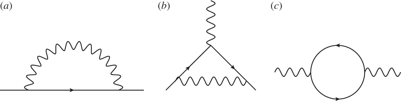
Figure 1: 1-loop divergent diagrams of QED. a) Electron self-energy, b) Vertex, c) Vacuum polarization.

In QED there are three primitively divergent diagrams depicted in Fig. 1. For anisotropic WSMs the same three diagrams give rise to various independent divergences due to anisotropy. Potentially divergent one–loop diagrams with with three and four external photon legs arising from LIV QED have been demonstrated to vanish in ref. KLP02.

Feynman diagrams of the model are constructed with the following propagators and vertex: rCl S_F(k) & = iγ0(k0-tk3)+ ∑i=13γiviki   ,
G_μν = iM_μν^-1   ,
V^μ = -iel^μ_νγ^ν   ,
l^μ_ν = ( 1 0 0 0 0 v10 0 0 0 v20 -t 0 0 v3 )   , and the matrix $M_{\mu\nu}$ is the one that appears when eq. (6) is rewritten as

$$\mathcal{L}_{\text{ph}}=\dfrac{1}{2}A^{\mu}M_{\mu\nu}A^{\nu}\ .$$ (7)

Symbolically, the electron self-energy, vacuum polarization and vertex diagrams are given by rCl Σ(p) &= ∫d4k(2π)4  V^μS_F(p-k)V^νG_μν(k)   ,
Π^μν(q) = -∫d4k(2π)4  Tr[ V^μS_F(k)V^νS_F(k-q) ] ,
Γ^μ(0,0) = ∫d4k(2π)4  V^aS_F(k)V^μS_F(k)V^bG_ab(k)   . A set of 13 counterterms are introduced in the parameters of the lagrangian to cancel the divergencies of these diagrams. Due to gauge invariance, not all are independent. We choose a renormalization of the polarization tensor such that neither the photon field $A_{\mu}$ nor the electric charge $e$ renormalize. The parameters $\epsilon_{i},\mu_{i}$ determine the renormalization of the speed of light in the different directions.

IV Beta functions and results

The beta functions of the parameters of the model are defined by $\beta_{x}\equiv dx/d(\log\Lambda)$, where $\Lambda$ is the energy scale introduced in the renormalization procedure. We have used a dimensional regularization scheme to define the counterterms described in Appendix LABEL:sec_ApRen which leads to the following beta functions rCCCCCCCl β_t = α_3ϵ_3 ( tF_0^0+F_3^0 ) ,    &β_v_i= α_iϵ_i( v_iF_0^0-F_i^i ) ,   i=1,2,3
  β_ω_1 = 2α13v1v2v3( ω_1-t )   ,  β_ω_2=2α23v2v1v3( ω_2-t )   ,
β_ϵ_1 = -2α13ϵ_1v1v2v3  ,   β_ϵ_2 = -2α23ϵ_2v2v1v3   ,    β_ϵ_3 = -2α33ϵ_3v3v1v2   ,  
β_μ_1 = 2α13ϵ_1μ_1^2v2(v32-(t-ω2)2)v1v3 ,    β_μ_2 = 2α23ϵ_2μ_2^2v1(v32-(t-ω1)2)v2v3 ,    β_μ_3 = 2α33ϵ_3μ_3^2v1v2v3   ,

In what follows we will analyze the RG flows of the most significant examples. The dimensionless coupling constants of our theory are given by $\alpha_{i}\equiv\alpha/\epsilon_{i}$ for $i=1,2,3$. They go to zero in the infrared limit in all the cases analyzed through the article.

IV.1 Isotropic case

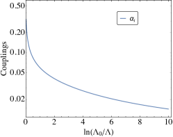
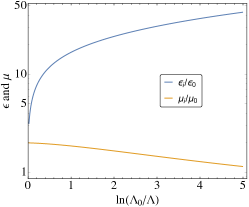
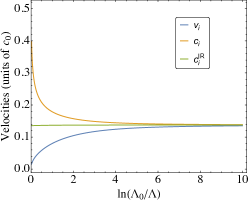
(a) (b)  (c)

Figure 2: Isotropic runnings of various parameters for the initial values $v_{i}=0.01,\;\epsilon_{i}=2,\;\mu_{i}=2,\;$ with $i=1,2,3$.

To fix the notation and as a consistency check we have first analyzed the isotropic case ($v_{i}=v$) without tilt. This case has already been studied in the literature IN12; RJH16. Our results are shown in Fig. 2 for the initial values given in the caption. The coupling constants go to zero in the infrared limit (Fig. 2 (a). We took $\alpha=1$ as initial value to compare with the results of ref. IN12 but the rapid decrease of the couplings ensures the validity of perturbation theory. The velocity of light in the isotropic case is and $c_{i}=1/\epsilon_{i}\mu_{i}$, $i=1,2,3$.

In Fig. 2(b) we show the running of the isotropic electric susceptibility $\epsilon$ and magnetic permittivity $\mu$. In all cases analyzed they run to infinity and zero respectively in the infrared and their product sets the running of the velocity of light $c$. In Fig. 2 (c) we show the running of the Fermi velocity and the velocity of light in the material. As we see, they converge to the same non–universal value which is approximately $c_{i}^{\text{IR}}=(c_{i}^{2}v_{i})^{1/3}$. This agrees with the results in IN12; RJH16.

IV.2 Anisotropic Fermi velocity and no tilt.

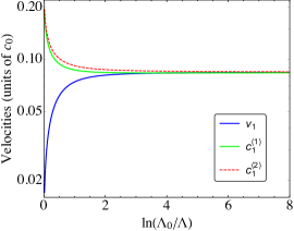
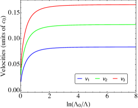
(a)  (b)

Figure 3: (a) Runnings of the fermion and photon velocities in the X direction in the anisotropic case with no tilt for the initial values are described in the text. Fermion and photon velocities converge to the same value at the infrared. The same happens in the Y and Z directions. (b) Comparative runnings of the Fermi velocities in the three directions. The asymptotic fixed point is anisotropic.

To our best knowledge this case has not been studied previously in the literature. Surprisingly, rotational symmetry is not recovered at the fixed point. Our results are shown in Fig. 3 for the initial values: rCllrCllrCllrCll α