Spatially adaptive image compression using a tiled deep network

Abstract

Deep neural networks represent a powerful class of function approximators that can learn to compress and reconstruct images. Existing image compression algorithms based on neural networks learn quantized representations with a constant spatial bit rate across each image. While entropy coding introduces some spatial variation, traditional codecs have benefited significantly by explicitly adapting the bit rate based on local image complexity and visual saliency. This paper introduces an algorithm that combines deep neural networks with quality-sensitive bit rate adaptation using a tiled network. We demonstrate the importance of spatial context prediction and show improved quantitative (PSNR) and qualitative (subjective rater assessment) results compared to a non-adaptive baseline and a recently published image compression model based on fully-convolutional neural networks.

Index Terms—  Image Compression, Neural Networks, Block-Based Coding, Spatial Context Prediction

1 Introduction

Many researchers have investigated the use of neural networks to learn models for lossy image compression (see [1] for a review) including a recent resurgence due to improved methods for training deep networks [2, 3, 4, 5]. These learned models produce compressed representations with a fixed bit rate across the image. Some spatial variation may be introduced by lossless entropy coding, which is applied as a post-process to compress the generated representation. This variation, however, is tied to the frequency and predictability of the codes, not directly to the complexity of the underlying visual information.

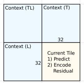
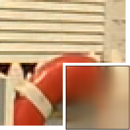
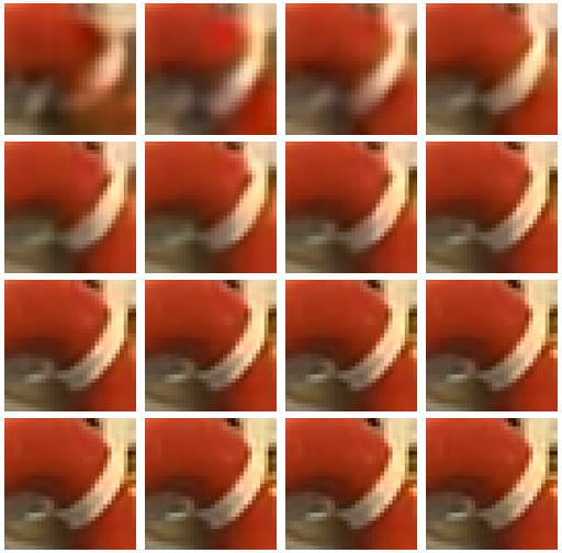
Fig. 1: For each $32\times 32$ tile, our model uses neighboring tiles above and to the left as context (left). First, a deep network predicts the pixel values for the target tile (center), and then a second network improves the reconstruction by progressively encoding the residual (right).

Traditional image codecs typically use both entropy coding and explicit bit rate adaptation that depends on local reconstruction quality (e.g., JPEG 2000, WebP, and BPG) [6, 7, 8, 9]. This spatial adaptation allows them to use additional bits more effectively by preferentially describing regions of the image that are more complex or visually salient.

This paper introduces an approach to image compression that combines the advantages of deep networks with bit rate adaptation based on local reconstruction quality. Neural networks provide two primary benefits for image compression: (1) they represent an extremely powerful, nonlinear class of regression functions (e.g., from pixel values to quantized codes and from codes back to pixels), and (2) their model parameters can be efficiently trained on large data sets. The second benefit is particularly important because it means that an effective architecture can be easily specialized to new domains and specific applications. For example, an architecture that works well on natural images can be retrained and optimized for cartoons, selfies, sketches, or presentations, where each domain contains images with substantially different statistics.

State of the art neural networks for image compression use fully-convolutional architectures [2, 3, 4, 5]. This design promotes efficient local information sharing and allows the networks to run on images with arbitrary resolution [10]. The tradeoff is that the shared dependence on nearby binary codes makes it difficult to adjust the bit rate across an image. Research done in parallel to this paper investigates ways to overcome this difficulty by using a more complex training procedure [11]. Our model, on the other hand, sidesteps the problem by using a block-based architecture. This tiled design maintains resolution flexibility and local information sharing while also significantly simplifying the implementation of bit rate adaptation.

2 Codec Overview

Our method works by dividing images into tiles, using spatial context to make an initial prediction of the pixel values within each tile, and then progressively encoding the residual. This approach is similar to the high-level structure of existing codecs such as WebP and BPG, though we use a fixed $32\times 32$ tiling while those methods use a more sophisticated process for adaptively subdividing each image.

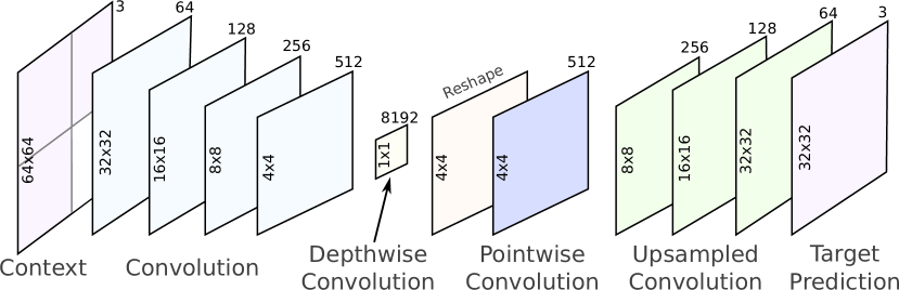
Fig. 2: The context prediction network uses strided convolution to extract features from the context tiles and uses upsampled convolution to generate an RGB prediction for the target tile. Each block in the diagram represents a layer in the neural network with the resolution shown inside the block and the depth (e.g., 3 for the RGB input and output) shown above.

Image encoding proceeds tile-by-tile in raster order. For each tile, the spatial context includes the neighboring tiles to the left and above (see Figure 1). This leads to a $64\times 64$ context patch where the values of the target tile (the bottom-right quadrant) has not yet been processed. The initial prediction for the target tile is produced by a neural network trained to analyze context patches and minimize the $L_{1}$ error between its prediction and the true target tile (details in Section 2.1). The goal is to take advantage of correlations between relatively distant pixels and thus avoid the cost of re-encoding visual information that is consistent from one tile to the next.

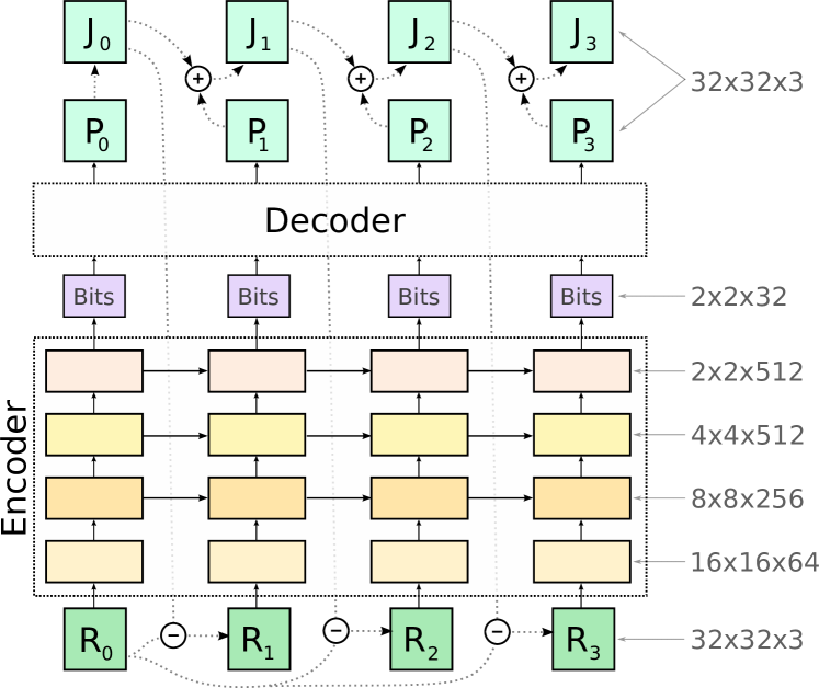
Fig. 3: The residual encoder uses a recurrent auto-encoder architecture where each layer has the shape shown (height $\times$ width $\times$ depth). Each iteration (four are shown) extracts features from its input ($R_{i}$) and quantizes them to generate 128 bits. The decoder learns to reconstruct the input from these binary codes. Each iteration tries to capture the residual remaining from the previous iteration so the sum across iteration outputs ($P_{i}$) provides a successively better approximation of the original input ($R_{0}\approx J_{i}=\sum_{k=0}^{i}P_{k}$).

Contextual data is unlikely to contain enough information to accurately reconstruct image details or to predict pixel values across object boundaries. The second step of our approach fills in such details by encoding the residual between the true image tile and the initial prediction using a deep network based on recurrent auto-encoders (details in Section 2.2). After a tile has been encoded, the decoded pixel values are stored and used as context for predicting subsequent tiles. This process repeats until all tiles have been processed.

2.1 Spatial Context Prediction

The spatial context predictor is a deep neural network that analyzes incomplete $64\times 64$ image patches and generates $32\times 32$ images that complete the original patch (see Figure 1). Our architecture is based on the work of Pathak et al. who developed a network that could inpaint missing tiles or random regions within a larger patch [12]. Whereas their method was trained to incorporate context from all directions, our network is trained exclusively to predict the lower-right quadrant of an image patch to support raster order encoding and decoding.

Figure 2 shows the architecture of our spatial context predictor network. The 3-channel context patch is taken as input and processed by four convolutional layers (stride = 2). Each of these layers learns a feature map with a reduced resolution and a higher depth. A “channel-wise, fully-connected” layer (as described in [12]) is implemented using a depthwise followed by a pointwise convolutional layer. The goal of this part of the network is to allow information to propagate across the entire tile without incurring the full quadratic cost of a fully-connected layer. For our network, a fully-connected layer would require 64 million parameters ($(4\times 4\times 512)^{2}$), whereas the channel-wise approach only requires 384 thousand ($4\times 4\times 8192+512\times 512$), a 170x reduction. The final stage of the network uses upsampled convolution (sometimes called “deconvolution”, “fractional convolution”, or “up-convolution”) to incrementally increase the spatial resolution until the last layer generates a 3-channel image from the preceding $32\times 32\times 64$ feature map.

2.2 Residual Encoding with Recurrent Networks

The context predictor typically generates accurate low-frequency data for each new tile, but it is not able to recover many image details. To improve reconstruction quality, the next step of our algorithm uses a second deep network that learns to compress and reconstruct residual images. The architecture of this network is based on recurrent auto-encoders and a binary bottleneck layer (see Figure 3). Specifically, we adopt the “LSTM (Additive Reconstruction)” architecture presented by Toderici et al. [2], except that where that paper trains the network to compress full images, we train it to compress the residual within each tile after running the context predictor.

Fig. 4: Block artifacts are visible when tiles are coded independently (left) but disappear when the spatial context predictor is used (right) [Best viewed zoomed in].

The encoder portion of the network uses one convolutional layer to extract features from the input residual image followed by three convolutional LSTM layers that reduce the spatial resolution (stride = 2) and generate feature maps. Weights are shared across all iterations, and the recurrent connections allow information to propagate from one iteration to the next. Our experiments showed that the recurrent connections were vital and that this architecture significantly outperformed a similar one made up of independent, non-recurrent auto-encoders.

The binary bottleneck layer maps incoming features to $\{-1,1\}$ using a $1\times 1$ convolution followed by a tanh activation function. Following the work of Raiko et al. on learning binary stochastic layers [13], we sample from the output of the tanh ($P(b=1)=0.5\cdot(1+tanh(x))$) to encourage exploration in parameter space. When we apply the trained network to images at run-time, however, we binarize deterministically ($b=sign(tanh(x))$ with $b=1$ when $x=0$).

The decoder sub-network has the same structure as the encoder, except upsampled convolution is used to increase the resolution of each feature map by $2\times$ in each layer. The final layer takes the output of the decoder (a feature map with shape $32\times 32\times 64$) and uses a tanh activation to map the features to three values in the range $[-1,1]$. The output is then scaled, clipped, and quantized to 8-bit RGB values ($R=round(min(max(R^{\prime}\cdot 142+128,0),255))$). Note that we scale by 142 instead of 128 to allow the network to more easily predict extreme pixel values without entering the range of tanh with tiny gradients, which can lead to slow learning.

2.3 Spatially Adaptive Bit Allocation

Adaptive bit allocation is difficult in existing neural network compression architectures because the models are fully-convolutional. If such networks are trained with all of the binary codes present, reconstruction with missing codes can be arbitrarily bad. Our approach avoids this problem by sharing information from the binary codes within each tile but not across tiles. This strategy allows the algorithm to safely reduce the bit rate in one area without degrading the quality of neighboring tiles.

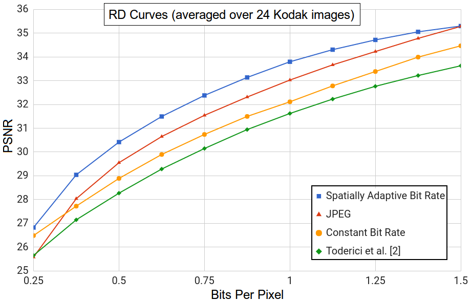
Fig. 5: Using a constant bit rate, our approach shows a small PSNR improvement over the method in [2] but only outperforms JPEG at very low bit rates. By adapting the bit rate to local image complexity, our method yields a higher mean PSNR across the full range (0.25 – 1.5 bpp).

One potential pitfall of a block-based codec is the possible emergence of boundary artifacts between tiles. The spatial context predictor helps avoid this problem by sharing information across tile boundaries without increasing the bit rate (see Figure 4). In essence, the context prediction network learns how to generate pixels that mesh well with their context. Furthermore, since the predicted pixels are more detailed and accurate near the context pixels, the network naturally acts to minimize border artifacts.

Our approach for allocating bits across each image is straightforward. During image encoding, each tile uses enough bits to exceed a specified target quality level (compared to a target bit rate in the constant bit rate case). The results presented below are based on a PSNR target, but any local quality or saliency measure can be used (see the bottom-right of Figure 6 for examples of bit rate maps).

2.4 Training and Run-Time Details

Both the spatial context predictor and residual encoder networks were implemented using Tensorflow [14] and trained using the Adam optimizer [15]. They are trained sequentially since the residual encoder network learns to encode the specific pixel errors that remain after context prediction. The training process used a mini-batch size of 32 and an initial learning rate of 0.5 following an exponential decay schedule ($\beta=0.95$) with a step size of 20,000.

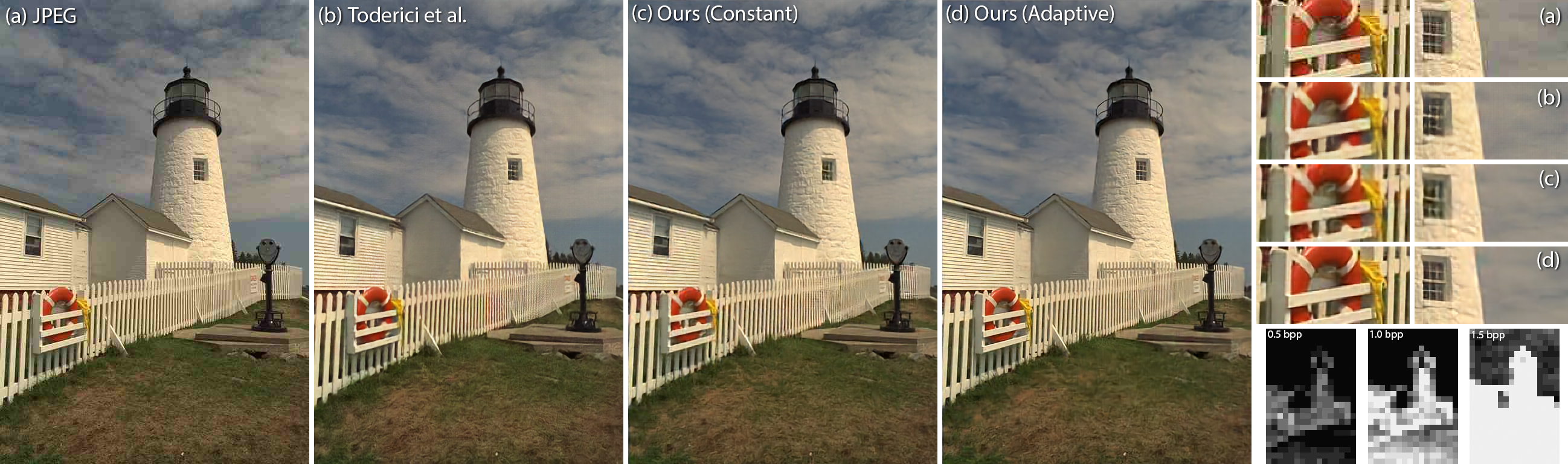
Fig. 6: Reconstructions at 0.5 bpp: (a) JPEG (PSNR=29.552), (b) Toderici et al. [2] (28.270), (c) our method with constant bit rate (28.890), and (d) our adaptive model (30.418). The far right (top) shows two zoomed-in regions for better comparison, while the bottom shows the adaptive bit rate mask calculated at three bit rates.

Our training data consists of $64\times 64$ image patches cropped from a collection of six million $1280\times 720$ public images from the web. Following the procedure described by Toderici et al. [2], we use the 100 patches from each image that were most difficult to compress as measured by the PNG codec.

At run-time, the encoder process monitors the reconstruction error of each tile and uses as few bits as possible to reach the target quality. This is possible because the residual encoder is a recurrent network and can be stopped after any step. Since each step generates additional bits, this mechanism allows adapitve bit allocation and allows a single neural network to generate encodings at different bit rates.

3 Results and Evaluation

We evaluated our approach with both quantitative and qualitative assessments using the the Kodak image set [16]. Figure 4 includes two crops coded at 0.375 bits per pixel (bpp) that show the impact of the spatial context predictor. Without it, each $32\times 32$ tile is coded independently and block artifacts are clearly visible.

The rate-distortion graph in Figure 5 shows PSNR values averaged over the 24 images in the Kodak data set. The results show that our approach outperforms the baseline neural network algorithm from [2] between 0.25 and 1.5 bpp. The spatially adaptive version of our algorithm further increases reconstruction quality and outperforms both of those models as well as JPEG [17] across this bit rate range.

Example images at 0.5 bpp are shown in Figure 6. JPEG shows significant block artifacts and color shifts (e.g., in the sky) not present in the other images. Both Toderici et al. and our constant bit rate reconstruction suffer from aliasing and a color shift on the fence, and neither reconstructs the life buoy or yellow rope with much detail. Our spatially adaptive method addresses all of these issues. Its reconstruction, however, does have less detail in some visually simple but salient areas (e.g., the mounted binoculars) and some neighboring regions have distracting differences in the amount of retained detail (e.g., where the fence meets the grass). More sophisticated criteria for bit allocation that better capture visual saliency will help in both cases and can be easily plugged in to our algorithm.

Ten raters subjectively evaluated our results over the Kodak image set in a pairwise study that included 24 images, four codecs, and six bit rates (0.25 – 1.5 in 0.25 bpp increments) for a total of 8,640 image comparisons. In all cases, the mean preferrence favored our adaptive algorithm over both the constant bit rate version and the neural network baseline from [2]. Our adaptive algorithm was also preferred to JPEG at 0.25 and 0.5 bpp; elsewhere, the differences were not statistically significant ($\alpha=0.05$).

4 Conclusion and Future Work

The primary goal of our current research is to combine deep neural networks with spatial bit rate adaptation, which we think is vital for state of the art compression results. By adopting a block-based approach, we are able to limit the extent of local information sharing, which allows us to easily incorporate a wide range of quality metrics to control local bit rate. Our experiments show that explicit bit rate adaptation increases both quantiative and subjective image quality assessments.

Our approach can be improved in many ways. Adaptively subdividing images instead of using fixed $32\times 32$ tiles will boost reconstruction quality but requires more flexible network architectures. We can also adopt a multiscale model where lower-resolution encodings act as a prior to guide the predictions at higher resolutions. Better criteria for bit allocation should yield significant quality improvements, particularly in terms of subjective assessment. Finally, practical deployment will require additional research to shrink the learned models and reduce their run-time requirements. Currently, although the models produce higher quality compression results than JPEG, their execution speed is much slower even when accelerated by modern GPU hardware.

References

- [1] J. Jiang, “Image compression with neural networks–a survey,” Signal Processing: Image Communication, vol. 14, pp. 737–760, 1999.
- [2] George Toderici, Damien Vincent, Nick Johnston, Sung Jin Hwang, David Minnen, Joel Shor, and Michele Covell, “Full resolution image compression with recurrent neural networks,” CoRR, vol. abs/1608.05148, 2016.
- [3] Johannes Ballé, Valero Laparra, and Eero P. Simoncelli, “End-to-end optimization of nonlinear transform codes for perceptual quality,” in Picture Coding Symposium, 2016.
- [4] George Toderici, Sean M O’Malley, Sung Jin Hwang, Damien Vincent, David Minnen, Shumeet Baluja, Michele Covell, and Rahul Sukthankar, “Variable rate image compression with recurrent neural networks,” ICLR, 2016.
- [5] K. Gregor, F. Besse, D. Jimenez Rezende, I. Danihelka, and D. Wierstra, “Towards Conceptual Compression,” in NIPS, 2016.
- [6] “Information technology–JPEG 2000 image coding system,” Standard, International Organization for Standardization, Geneva, CH, Dec. 2000.
- [7] Google, “WebP: Compression techniques (http://developers.google.com/speed/webp/docs/compression),” Accessed: 2017-01-30.
- [8] F. Bellard, “BPG image format (http://bellard.org/bpg/),” Accessed: 2017-01-30.
- [9] David R. Bull, Ed., Communicating Pictures: A Course in Image and Video Coding, Academic Press, Oxford, 2014.
- [10] J. Long, E. Shelhamer, and T. Darrell, “Fully convolutional networks for semantic segmentation,” CoRR, vol. abs/1411.4038, 2014.
- [11] M. Covell, N. Johnston, D. Minnen, S.J. Hwang, J. Shor, S. Singh, D. Vincent, and G. Toderici, “Target-quality image compression with recurrent, convolutional neural networks,” CoRR, vol. abs/1705.06687, 2017.
- [12] Deepak Pathak, Philipp Krähenbühl, Jeff Donahue, Trevor Darrell, and Alexei Efros, “Context encoders: Feature learning by inpainting,” in CVPR, 2016.
- [13] T. Raiko, M. Berglund, G. Alain, and L. Dinh, “Techniques for learning binary stochastic feedforward neural networks,” ICLR, 2015.
- [14] Martín Abadi, Ashish Agarwal, Paul Barham, Eugene Brevdo, Zhifeng Chen, Craig Citro, Greg S. Corrado, Andy Davis, Jeffrey Dean, Matthieu Devin, Sanjay Ghemawat, Ian Goodfellow, Andrew Harp, Geoffrey Irving, Michael Isard, Yangqing Jia, Rafal Jozefowicz, Lukasz Kaiser, Manjunath Kudlur, Josh Levenberg, Dan Mané, Rajat Monga, Sherry Moore, Derek Murray, Chris Olah, Mike Schuster, Jonathon Shlens, Benoit Steiner, Ilya Sutskever, Kunal Talwar, Paul Tucker, Vincent Vanhoucke, Vijay Vasudevan, Fernanda Viégas, Oriol Vinyals, Pete Warden, Martin Wattenberg, Martin Wicke, Yuan Yu, and Xiaoqiang Zheng, “TensorFlow: Large-scale machine learning on heterogeneous systems,” 2015, Software available from tensorflow.org.
- [15] D. P. Kingma and J. Ba, “Adam: A method for stochastic optimization,” CoRR, vol. abs/1412.6980, 2014.
- [16] Eastman Kodak, “Kodak lossless true color image suite (PhotoCD PCD0992),” .
- [17] W. Pennebaker and J. Mitchell, JPEG: Still Image Compression Standard, Kluwer Academic Publishers, 1992.