Action-based dynamical models of dwarf spheroidal galaxies: application to Fornax

Abstract

We present new dynamical models of dwarf spheroidal galaxies (dSphs) in which both the stellar component and the dark halo are described by analytic distribution functions that depend on the action integrals. In their most general form these distribution functions can represent axisymmetric and possibly rotating stellar systems. Here, as a first application, we model the Fornax dSph, limiting ourselves, for simplicity, to the non rotating, spherical case. The models are compared with state-of-the-art spectroscopic and photometric observations of Fornax, exploiting the knowledge of the line-of-sight velocity distribution of the models and accounting for the foreground contamination from the Milky Way. The model that best fits the structural and kinematic properties of Fornax has a cored dark halo, with core size $r_{\rm c}\simeq 1.03$ kpc. The dark-to-luminous mass ratio is $(M_{\rm dm}/M_{\star})|_{R_{\rm e}}\simeq 9.6$ within the effective radius $R_{\rm e}\simeq 0.62\,$kpc and $(M_{\rm dm}/M_{\star})|_{3{\rm kpc}}\simeq 144$ within 3 kpc. The stellar velocity distribution is isotropic almost over the full radial range covered by the spectroscopic data and slightly radially anisotropic in the outskirts of the stellar distribution. The dark-matter annihilation $J$-factor and decay $D$-factor are, respectively, $\log_{10}(J$ $[$GeV² cm${}^{-5}])\simeq 18.34$ and $\log_{10}(D$ $[$GeV cm${}^{-2}])\simeq 18.55$, for integration angle $\theta=0.5^{\circ}$. This cored halo model of Fornax is preferred, with high statistical significance, to both models with a Navarro, Frenk and White dark halo and simple mass-follows-light models.

1 Introduction

The dwarf spheroidal galaxies (dSphs) are gas poor faint stellar systems with roughly elliptical shape. Due to their very low surface brightness, dSphs are observed only in the local Universe, but similar galaxies are expected to be ubiquitous in the cosmos. The nearest and best known dSphs belong to the Local Group, being satellites of the Milky Way (hereafter MW) and M31. dSphs are interesting astrophysical targets for several reasons. In the standard $\Lambda$ cold dark matter ($\Lambda$CDM) cosmological model, dwarf galaxies are the building blocks of more massive galaxies, so the knowledge of their properties is a fundamental step in understanding galaxy formation. Moreover, there is now much evidence (essentially based on measures of the stellar line-of-sight velocities; Aaronson 1983, Battaglia et al. 2013) that these galaxies are hosted in massive and extended dark halos, which usually dominate the stellar components even in the central parts. dSphs almost completely lack emission in bands other than the optical, so they are natural locations at which to look for high-energy signals from annihilating or decaying dark-matter particles (e.g. Evans et al. 2016). These facts make dSphs ideal laboratories in which to study dark matter, to understand the processes that drive galaxy formation and to test cosmology on the smallest scales, where there is potential tension between the observational data and the predictions of the $\Lambda$CDM model (Bullock & Boylan-Kolchin 2017).

The core/cusp problem is a clear example of this controversy: on the one hand, cosmological dark-matter only $N$-body simulations predict cuspy dark halo density profiles; on the other hand, the rotation curves of low surface brightness disc and gas-rich dwarf galaxies favour shallower or cored dark-matter density distributions (de Blok 2010 and references therein). Also for dSphs, for which the determination of the dark-matter density distribution is more difficult, there are indications that cored dark-matter density profiles may be favoured with respect to cuspy profiles (Kleyna et al. 2003, Goerdt et al. 2006, Battaglia et al. 2008, Walker & Peñarrubia 2011, Salucci et al. 2012, Amorisco et al. 2013, Zhu et al. 2016), though this finding is still debated (Richardson & Fairbairn 2014, Strigari et al. 2017). It must be stressed, however, that cored dark halos in dSphs do not necessarily imply a failure of $\Lambda$CDM: DM-only cosmological simulations may not reliably predict the present-day dark-matter distribution in dSphs because, by definition, they neglect the effects of baryons on the dark halos. Even in a galaxy that is everywhere dark-matter dominated today, baryons must have been locally dominant in the past to permit star formation. Therefore, the effect of baryon physics on the dark halo is expected to be important also in dSphs. For instance, Nipoti & Binney (2015) showed how, due to the fragmentation of a disc in cuspy dark halo, dynamical friction may cause the halo to flatten the original cusp into a core even before the formation of the first stars (see also El-Zant et al. 2001, Mo & Mao 2004, Goerdt et al. 2010, Cole et al. 2011, Arca-Sedda & Capuzzo-Dolcetta 2017). Moreover, the results of hydrodynamical simulations suggest that, following star formation, supernova feedback can also help to flatten the central dark-matter distribution, by expelling the gas (Navarro et al. 1996a, Read & Gilmore 2005) and thus inducing rapid fluctuations in the gravitational potential (Mashchenko et al. 2006, Pontzen & Governato 2012, Tollet et al. 2016).

The determination of the dark-matter distribution in observed dSphs relies on the combination of high-quality observational data and sophisticated dynamical modelling (see Battaglia et al. 2013 for a review). With the advent of the latest generation of spectrographs and thanks to wide-field surveys, today we have relatively large samples of individual stars in dSphs with measured line-of-sight velocities, allowing, in principle, for a detailed study of the dynamics of these nearby dwarf galaxies. To exploit this kind of information optimally, much effort has gone into developing reliable, physical and self-consistent techniques for modelling galaxies (Strigari et al. 2008, Walker et al. 2009, Amorisco & Evans 2011, Jardel & Gebhardt 2012, Breddels & Helmi 2013). However, the process of understanding the properties of the dark halos of dSphs is far from complete.

If the effects of the tidal field of the host galaxy (for instance the MW) are negligible, a dSph can be modeled as a collisionless equilibrium stellar system, which is completely described in terms of time-independent distribution functions (hereafter DFs). In this work we present a novel mass modelling method for dSphs based on DFs depending on the action integrals ${\bf J}$. The actions are integrals of motion that can be complemented by canonically conjugate (angle) variables to form a set of phase-space canonical coordinates. The action $J_{i}$ is

$$J_{i}=\frac{1}{2\pi}\oint_{\gamma_{i}}{\bf p}\cdot\text{d}{\bf q},$$ (1)

where ${\bf p}$ and ${\bf q}$ are any canonical phase-space coordinates and $\gamma_{i}$ is a closed path over which the corresponding angle conjugate to $J_{i}$ makes a full oscillation. Actions are ideal labels for stellar orbits, and an action-based DF specifies how the galaxy’s orbits are populated. Binney (2014) proved that spherical galaxy models based on $f({\bf J})$ DFs depending on actions can easily be extended to systems with rotation and flattening. Moreover, actions are adiabatic invariants (i.e. they are unchanged under slow changes in the potential). This property makes the $f(\bf J)$ models particularly suitable to model multi-component galaxies, in which some components may have grown adiabatically. For instance, during the accumulation of the baryonic component in a dark halo, the total gravitational potential changes, and so does the halo’s density distribution. However, if the halo responds adiabatically, the distribution of its particles in action space remains unchanged.

Regardless of whether a galaxy is really assembled by adiabatic addition of components, one can readily assign each component a likely action-based DF that completely specifies the component’s mass and angular momentum, and then quickly solve for the gravitational potential that all components jointly generate (Piffl et al. 2015). Once that is done, it is easy to compute any observable whatsoever. Thanks to all of these features, dynamical models relying on action-based DFs have proved successful in modelling the MW (Piffl et al. 2015, Binney & Piffl 2015, Sanders & Evans 2015, Cole & Binney 2017).

The application of the $f({\bf J})$ models to dSphs is also very promising, because it exploits the possibility of computing physical models with known DFs, given large kinematic samples of line-of-sight velocity measures (see Williams & Evans 2015, Jeffreson et al. 2017). In particular, given that for our models we can compute the line-of-sight velocity distribution, we can use it to build up a Maximum Likelihood Estimator (MLE) based on measures of velocities of individual stars, thus eliminating any kind of information loss due to binning the kinematic data (Watkins et al. 2013).

As a first application, in this paper we apply $f({\bf J})$ models to the Fornax dSph, which was the first to be discovered (Shapley 1938). Fornax is located at high Galactic latitude at a distance of $138\pm 8\,$kpc (Mateo 1998; Battaglia et al. 2006), and has the largest body of kinematic data. There are quantitative indications (Battaglia et al. 2015) that the effect of the tidal field of the Milky Way on the present-day dynamics of Fornax is negligible, so we are justified in modelling this galaxy as a stationary isolated stellar system.

This paper is organised as follows: in Section 2 we introduce the DF that we propose for dSphs and summarise the main characteristics of the models it generates. In Sections 3 models are compared to observations of dSphs. In Section 4 we present the results obtained applying our technique to the Fornax dSphs. Section 5 concludes.

2 two-component $f({\bf J})$ models for dwarf spheroidal galaxies

We model a dSph as a two-component system with stars and dark matter.

2.1 Stellar component

The stellar component is described by the DF

$$f_{\star}({\bf J})=\frac{M_{0,\star}}{J_{0,\star}^{3}}\exp\biggl{[}-\biggl{(}\frac{k({\bf J})}{J_{0,\star}}\biggr{)}^{\alpha}\biggr{]},$$ (2)

with

$$k({\bf J})=J_{r}+\eta_{\phi}|J_{\phi}|+\eta_{z}J_{z},$$ (3)

where ${\bf J}=(J_{r},J_{\phi},J_{z})$ comprises $J_{r}$, the radial action, $J_{\phi}$, the azimuthal action, and $J_{z}$ the vertical action, $M_{0,\star}$ is a characteristic mass, $J_{0,\star}$ is a characteristic action, and $\alpha$, $\eta_{\phi}$ and $\eta_{z}$ are dimensionless, non-negative, parameters. The DF in equation (2) proves to be expedient in representing dSph since it generates an almost exponential cut-off in the density distribution, similar to what is observed for typical dSphs (Irwin & Hatzidimitriou 1995).

2.2 Dark-matter component

We consider a family of DFs for the dark halo such that, in the absence of baryons, the dark-matter density distribution is very similar to an exponentially truncated Navarro, Frenk & White (1996b, hereafter NFW) profile, with the optional presence of a central core. Specifically, the dark-matter component is described by the DF

$$f_{\rm dm}({\bf J})=f({\bf J})g({\bf J})T({\bf J}),$$ (4)

where

$$f({\bf J})=\frac{M_{0,\rm dm}}{J_{0,\rm dm}^{3}}\frac{[1+J_{0,\rm dm}/h({\bf J})]^{5/3}}{[1+h({\bf J})/J_{0,\rm dm}]^{2.9}},$$ (5)

$$g({\bf J})=\biggl{[}\biggl{(}\frac{J_{\rm c,dm}}{h({\bf J})}\biggr{)}^{2}-\mu\frac{J_{\rm c,dm}}{h({\bf J})}+1\biggr{]}^{-5/6}$$ (6)

and

$$T({\bf J})=\exp{\biggl{[}-\biggl{(}\frac{h({\bf J})}{J_{\rm t,dm}}\biggr{)}^{2}\biggr{]}}.$$ (7)

Here, $M_{0,\rm dm}$ is a characteristic mass scale and $J_{0,\rm dm}$ is a characteristic action scale, while $h({\bf J})$ is the homogeneous function of the actions

$$h({\bf J})=J_{r}+\delta_{h,\phi}|J_{\phi}|+\delta_{h,z}J_{z},$$ (8)

where $\delta_{h,\phi}$ and $\delta_{h,z}$ are dimensionless, non-negative, parameters regulating the velocity distribution of the halo. Posti et al. (2015) introduced the DF (5) to describe NFW-like $f({\bf J})$ models . To avoid the divergence of the dark-matter mass for large actions we multiply the DF by the exponential term (7), in which $J_{\rm t,dm}$ is a characteristic action that determines the spatial truncation of the density distribution. Following Cole & Binney (2017), in equation (4) the DF of Posti et al. (2015) is multiplied by the function $g({\bf J})$ in order to produce a core in the innermost regions of the dark-matter density distribution. The size of the core is regulated by the characteristic action $J_{\rm c,dm}$. The dimensionless parameter $\mu$ is used to make the integral of the DF of (4) independent of $J_{\rm c,dm}$: the value of $\mu$ is such that models with different $J_{\rm c,dm}$, but with the same values of the other parameters of the DF (4), have the same total dark-matter mass.

2.3 General properties of the models

The total mass of each component is fully determined by the properties of its DF and is independent of the presence and properties of the other component (Binney 2014). The total stellar mass is

$$M_{\rm tot,\star}=(2\pi)^{3}\int f_{\star}({\bf J})\text{d}^{3}{\bf J},$$ (9)

while the total dark-matter mass is

$$M_{\rm tot,dm}=(2\pi)^{3}\int f_{\rm dm}({\bf J})\text{d}^{3}{\bf J}.$$ (10)

The stellar and dark-matter density distributions are, respectively,

$$\rho_{\star}({\bf x})=\int f_{\star}({\bf J}){\rm d}^{3}{\bf v}$$ (11)

and

$$\rho_{\rm dm}({\bf x})=\int f_{\rm dm}({\bf J}){\rm d}^{3}{\bf v}.$$ (12)

Evaluation of the integrals (11) and (12) involves the evaluation of the action ${\bf J}$ as functions of the ordinary phase-space coordinates $({\bf x},{\bf v})$ in the total gravitational potential $\Phi_{\text{tot}}=\Phi_{\star}+\Phi_{\text{dm}}$, where $\Phi_{\star}$ is the stellar gravitational potential, given by $\nabla^{2}\Phi_{\star}=4\pi G\rho_{\star}$, and $\Phi_{\text{dm}}$ is the dark-matter gravitational potential, given by $\nabla^{2}\Phi_{\text{dm}}=4\pi G\rho_{\rm dm}$. Thus, the problem is non-linear and the density-potential pairs $(\rho_{\star},\Phi_{\star})$ and $(\rho_{\rm dm},\Phi_{\text{dm}})$ are computed iteratively (see Binney 2014 , Posti et al. 2015 and Sanders & Binney 2016). Both DFs (2) and (4) are even in $J_{\phi}$, so they define non rotating models. Putting any component in rotation is straightforward following, for instance, the procedure described in Binney (2014). For non-rotating models, the velocity dispersion tensor of the stellar component is

$$\sigma^{2}_{i,j}\equiv\frac{\int v_{i}v_{j}f_{\star}({\bf J}){\rm d}^{3}{\bf v}}{\rho_{\star}(\bf x)},$$ (13)

where $v_{i}$ and $v_{j}$ are the $i$-th and $j$-th components of the velocity.

The characteristic length and velocity scales of the stellar component are, respectively,

$$r_{0,\star}\equiv\frac{J_{0,\star}^{2}}{GM_{0,\star}}$$ (14)

and

$$v_{0,\star}\equiv\frac{GM_{0,\star}}{J_{0,\star}}.$$ (15)

The characteristic length and velocity scales of the dark halo are, respectively,

$$r_{0,\rm dm}\equiv\frac{J_{0,\rm dm}^{2}}{GM_{0,\rm dm}}=\biggl{(}\frac{J_{0,\rm dm}}{J_{0,\star}}\biggr{)}^{2}\frac{M_{0,\star}}{M_{0,\rm dm}}r_{0,\star}=\frac{\tilde{J}_{0,\rm dm}^{2}}{\tilde{M}_{0,\rm dm}}r_{0,\star}$$ (16)

and

$$v_{0,\rm dm}\equiv\frac{GM_{0,\rm dm}}{J_{0,\rm dm}}=\frac{M_{0,\rm dm}}{M_{0,\star}}\frac{J_{0,\star}}{J_{0,\rm dm}}v_{0,\star}=\frac{\tilde{M}_{0,\rm dm}}{\tilde{J}_{0,\rm dm}}v_{0,\star},$$ (17)

where $\tilde{M}_{0,\rm dm}\equiv M_{0,\rm dm}/M_{0,\star}$ and $\tilde{J}_{0,\rm dm}\equiv J_{0,\rm dm}/J_{0,\star}$.

2.4 Spherical models

The simplest models belonging to the family described in Sections 2.1 and 2.2 are those in which both the dark-matter and the stellar components are spherically symmetric ($\eta_{\phi}=\eta_{z}$ in equation 2, and $\delta_{h,\phi}=\delta_{h,z}$, in equation 8). In general neither component is spherical if $\delta_{h,\phi}\neq\delta_{h,z}$ or $\eta_{\phi}\neq\eta_{z}$. Here we focus on the spherical case and define

$$\eta\equiv\eta_{\phi}=\eta_{z}$$ (18)

and

$$\delta\equiv\delta_{\phi,h}=\delta_{z,h}.$$ (19)

We require the dark-matter velocity distribution to be almost isotropic setting $\delta\leq 1$ (Posti et al. 2015). With these assumptions each of our models depends on the eight parameters

$$\boldsymbol{\xi}\equiv(\alpha,\eta,\tilde{M}_{0,\rm dm},\tilde{J}_{0,\rm dm},\tilde{J}_{\rm c,dm},\tilde{J}_{\rm t,dm},M_{0,\star},J_{0,\star}),$$ (20)

where $\tilde{J}_{\rm c,dm}\equiv J_{\rm c,dm}/J_{0,\rm dm}$ and $\tilde{J}_{\rm t,dm}\equiv J_{\rm t,dm}/J_{0,\rm dm}$. Models that share the dimensionless parameters $\alpha$, $\eta$, $\tilde{M}_{0,\rm dm}$, $\tilde{J}_{0,\rm dm}$, $\tilde{J}_{\rm c,dm}$ and $\tilde{J}_{\rm t,dm}$ are homologous. The physical units are determined by the dimensional parameters $M_{0,\star}$ and $J_{0,\star}$.

The stellar density distribution is characterised by an extended core and a truncation of adjustable steepness in the outskirts (see Section 4). For the stellar component we define the half-mass radius $r_{\rm h}$ as the radius of the sphere that contains half of the total stellar mass. The most general spherical $f({\bf J})$ model of Section 2.2 generates a dark-matter density profile characterised by three regimes: a core where the logarithmic slope of the density profile $\gamma\equiv\text{d}\ln\rho_{\rm dm}/\text{d}r\sim 0$, an intermediate region where $\gamma\sim-1$ and the outer region where $\gamma\sim-3$. For each model we define the core radius $r_{\rm c}\equiv r_{-1/2}$ (radius at which $\gamma=-1/2$), the scale radius $r_{\rm s}\equiv r_{-2}$ (radius at which $\gamma=-2$, as for the scale radius of the classical NFW model), and the truncation radius $r_{\rm t}\equiv r_{-3}$ (radius at which $\gamma=-3$).

The eight parameters $\boldsymbol{\xi}$ (equation 20) are quantities appearing in the DFs (equations 2 and 4) or combinations thereof (see Section 2.3). Once a model is computed, it can be also characterised by the eight parameters

$$\boldsymbol{\xi}^{\prime}=(\alpha,\eta,\tilde{M}_{\rm tot,dm},\tilde{r}_{\rm s},\tilde{r}_{\rm c},\tilde{r}_{\rm t},M_{0,\star},J_{0,\star}),$$ (21)

where we have replaced $\tilde{M}_{0,\rm dm}$, $\tilde{J}_{0,\rm dm}$, $\tilde{J}_{\rm c,dm}$ and $\tilde{J}_{\rm t,dm}$ with $\tilde{M}_{\rm tot,dm}\equiv M_{\rm tot,dm}/M_{\rm tot,\star}$, $\tilde{r}_{\rm s}\equiv r_{\rm s}/r_{\rm h}$, $\tilde{r}_{\rm c}\equiv r_{\rm c}/r_{\rm h}$, $\tilde{r}_{\rm t}\equiv r_{\rm t}/r_{\rm h}$, which have a more straightforward physical interpretation. In the following we briefly comment on the six dimensionless parameters $\alpha$, $\eta$, $\tilde{M}_{\rm tot,dm}$, $\tilde{r}_{\rm s}$, $\tilde{r}_{\rm c}$ and $\tilde{r}_{\rm t}$.

• $\alpha$: this mainly regulates the shape of the density profile of the stellar component. We find empirically that for higher values of $\alpha$ the core is flatter and the outer profile is steeper. This is expected because for higher values of $\alpha$ the DF (2) is more rapidly truncated for large actions.

• $\eta$: this mainly regulates the velocity anisotropy of the stellar component. We find empirically that higher values of $\eta$ generate more radially biased models. This is expected because orbits with large $|J_{\phi}|$ or $J_{z}$ are penalized for large values of $\eta$ (see equations 2 and 3; we recall that for spherical models $\eta_{\phi}=\eta_{z}=\eta$).

• $\tilde{M}_{\rm tot,dm}$: this is the ratio between the total dark-matter mass $M_{\rm tot,dm}$ and the total mass of the stellar component $M_{\rm tot,\star}$. Both $M_{\rm tot,dm}$ and $M_{\rm tot,\star}$ are well defined because the integrals in equations (9) and (10) converge. Since the DFs (2) and (4) depend on homogeneous functions of the actions, for spherical models the total masses are given by the one-dimensional integrals (Posti et al. 2015)

  $$\frac{M_{\rm tot,dm}}{M_{0,\rm dm}}=\frac{(2\pi)^{3}}{\delta^{2}}\int_{0}^{\infty}h^{2}f_{\rm dm}(h)\text{d}h$$ (22)

  for the dark halo, and

  $$\frac{M_{\rm tot,\star}}{M_{0,\star}}=\frac{(2\pi)^{3}}{\eta^{2}}\int_{0}^{\infty}h^{2}f_{\star}(h)\text{d}h$$ (23)

  for the stellar component (for details, see Appendix A). Given that $\tilde{M}_{\rm tot,dm}=M_{\rm tot,dm}/M_{\rm tot,\star}$, equations (22) and (23) can be combined to give

  $$\tilde{M}_{\rm tot,dm}=\tilde{M}_{0,\rm dm}\frac{\eta^{2}}{\delta^{2}}\frac{\int_{0}^{\infty}h^{2}f_{\rm dm}(h)\text{d}h}{\int_{0}^{\infty}h^{2}f_{\star}(h)\text{d}h}.$$ (24)

  The dark-matter to stellar mass ratio can be fixed by adjusting $\tilde{M}_{0,\rm dm}$ and $\mu$, the normalization parameter appearing in the definition of $f_{\rm dm}$ (see equations 4 and 6).

• $\tilde{r}_{\rm s}$: this is the ratio between the scale radius of the halo $r_{\rm s}$ and the half-mass radius of the stellar component $r_{\rm h}$. For sufficiently large $\tilde{r}_{\rm s}$, the dark-matter density profile is essentially a power law in the region populated by stars. This property makes the characteristic scale radius $r_{\rm s}$ and the normalisation of the dark-matter component degenerate: provided $\tilde{r}_{\rm s}\gg 1$, dark-matter density profiles with different values of $r_{\rm s}$ affect the stellar component in the same way, if properly scaled. Differently from $\tilde{M}_{\rm tot,dm}$, $\tilde{r}_{\rm s}$ cannot be fixed a priori since it depends on the total gravitational potential $\Phi_{\text{tot}}$. However, a model with a predefined value of $\tilde{r}_{\rm s}$ can be obtained iteratively.

• $\tilde{r}_{\rm c}$: this is the ratio between the core radius of the dark-matter component $r_{\rm c}$ and the half-mass radius of the stellar component $r_{\rm h}$. $\tilde{r}_{\rm c}$ cannot be fixed a priori because it depends on $\Phi_{\text{tot}}$. However, for the two-component models here considered, we find empirically that $\tilde{r}_{\rm c}$ can anyway be fixed with reasonable precision by fixing $\tilde{J}_{\rm c,dm}$.

• $\tilde{r}_{\rm t}$: this is the ratio between the truncation radius of the halo $r_{\rm t}$ and the half-mass radius of the stellar component $r_{\rm h}$. $\tilde{r}_{\rm t}$ depends on $\Phi_{\text{tot}}$, so it cannot be fixed a priori. In general, models with the same value of truncation action $\tilde{J}_{\rm t,dm}$ do not have the same value of $\tilde{r}_{\rm t}$.

3 STATISTICAL ANALYSIS

3.1 Comparison with data

When applying the spherical models presented in Section 2.4 to an observed dSph galaxy, the best model (i.e. the best set of eight parameters $\boldsymbol{\xi}$) is determined through a comparison with a set of observables. The dSph may be elliptical on the sky while our model will be spherical, so we assign each star a circularised radius

$$R\equiv\sqrt{x^{2}(1-\epsilon)+\frac{y^{2}}{(1-\epsilon)}},$$ (25)

where $\epsilon\equiv 1-b/a$, with $b$ and $a$ the lengths of the semi-minor and semi-major axes, is the ellipticity of the galaxy’s image on the sky and $(x,y)$ are the star’s Cartesian coordinates in the reference frame aligned with the image’s principal axes.

We assume the data comprises a photometric sample, used to compute the projected stellar number density $n_{\star}^{\text{obs}}$, and a kinematic sample with measurements of the line-of-sight velocities $v_{\rm los}$ of individual stars. We refer to the observed number density as a set of $N_{n}$ observed values $\{R_{i},n_{\star,i}^{\text{obs}}\}$, with $i=1,..,N_{n}$, and to the line-of-sight velocities as $N_{v}$ measures $\{R_{k},v_{{\rm los},k}\}$, with $k=1,..,N_{v}$. For each model we compute the stellar surface number density distribution

$$n_{\star}({\bf x}_{\perp})=\frac{N_{\rm tot,\star}}{M_{\rm tot,\star}}\int\rho_{\star}({\bf x})\text{d}x_{||},$$ (26)

where $N_{\rm tot,\star}$ is the total number of stars of the photometric sample, and the model line-of-sight velocity distribution (hereafter LOSVD)

$${\mathscr{L}}_{\star}({\bf x}_{\perp},v_{||})=\frac{\int f_{\star}[{\bf J}({\bf x},{\bf v})]\text{d}x_{||}\text{d}{\bf v}_{\perp}}{\rho_{\star}({\bf x}_{\perp})}.$$ (27)

Here, $x_{||}\equiv{\bf x}\cdot{\bf\hat{s}}$ and ${\bf x}_{\perp}={\bf x}-x_{||}{\bf\hat{s}}$ are, respectively, the parallel and orthogonal components of the position vector with respect to the line-of-sight (unit) vector ${\bf\hat{s}}$, and $v_{||}$ is the velocity component along ${\bf\hat{s}}$. For spherical models $n_{\star}$ and ${\mathscr{L}}_{\star}$ depend on ${\bf x}_{\perp}$ only through the scalar projected distance from the center on the plane of sky $R\equiv||{\bf x}_{\perp}||$.

We compare models to data with a maximum likelihood method. The log-likelihood of a model is defined as

$$\ln\mathcal{L}=\ln\mathcal{L}_{n}+\ln\mathcal{L}_{v},$$ (28)

with

$$\ln\mathcal{L}_{n}=-\frac{1}{2}\sum_{i=1}^{N_{n}}\biggl{(}\frac{n_{\star,i}^{\text{obs}}-n_{\star}(R_{i})}{\delta n_{i}}\biggr{)}^{2},$$ (29)

where $\delta n_{i}$ are the uncertainties of the stellar number density measurements, and

$$\ln\mathcal{L}_{v}=\sum_{k=1}^{N_{v}}\ln(p_{v,k}).$$ (30)

In the above equation

$$p_{v,k}\equiv\int_{-\infty}^{+\infty}{\mathscr{L}}_{\rm tot}(R_{k},v_{||})G_{k}(v_{||}-v_{{\rm los},k})\text{d}v_{||}$$ (31)

is the convolution of the total LOSVD ${\mathscr{L}}_{\rm tot}$ and a Gaussian distribution $G_{k}$ with null mean and standard deviation equal to the uncertainty on the line-of-sight velocity of the $k$-th star. The total LOSVD

$${\mathscr{L}}_{\rm tot}\equiv(1-\omega_{k}){\mathscr{L}}_{\star}+\omega_{k}{\mathscr{L}}_{{\rm f},k}$$ (32)

accounts for the fact that the kinematic sample of stars may be contaminated by field stars:

$${\mathscr{L}}_{{\rm f},k}\equiv{\mathscr{L}}_{{\rm f}}(v_{{\rm los},k})$$ (33)

is the LOSVD ${\mathscr{L}}_{\rm f}$ of field stars evaluated at $v_{{\rm los},k}$ and

$$\omega_{k}\equiv\frac{n_{\rm f}}{n_{\star}^{\text{obs}}(R_{k})+n_{\rm f}}$$ (34)

weights the relative contribution between dSph and contaminants. $n_{\rm f}$ is the mean projected number density of field stars, which is taken to be constant throughout the extent of the galaxy, while $n_{\star}^{\text{obs}}(R_{k})$ is the observed projected number density profile evaluated at $R_{k}$.

3.2 Models and families of models

$\Delta\ln\mathcal{L}_{j,m}$	$j=1$	$j=2$	$j=3$	$j=4$	$j=5$	$j=6$
$m=1$	0.50	1.15	1.77	2.36	2.95	3.52
$m=2$	2.00	4.01	4.85	4.85	5.65	6.40
$m=3$	3.00	5.90	7.10	8.15	9.10	10.05

Table 1: Values of the delta log-likelihood $\Delta\ln\mathcal{L}_{j,m}$ (equation 35) corresponding to $m\sigma$ confidence levels. $j$ is the number of free parameters of a family of models.

In the terminology used in this work, we distinguish the terms model and family of models. We refer to a class of spherical systems with the same values of the six dimensionless parameters ($\alpha$, $\eta$, $\tilde{M}_{0,\rm dm}$, $\tilde{J}_{0,\rm dm}$, $\tilde{J}_{\rm c,dm}$, $\tilde{J}_{\rm t,dm}$) as a model. Each model maps a two dimensional sub-space ($J_{0,\star},M_{0,\star}$) of homogeneous systems. When a model is compared with observations, we find the values of $J_{0,\star}$ and $M_{0,\star}$ that maximise $\mathcal{L}$ (equation 28) and, with a slight abuse of the terminology, we define its likelihood as this maximum value of $\mathcal{L}$.

We will refer to a set of models sharing some properties (i.e. values of some parameters) as a family of models. For instance, we will define the family of one-component (or mass-follows-light, MFL) models as the set of all models with $M_{0,\rm dm}=0$. Each family of models has $j$ free parameters, which we indicate with the $j$-dimensional vector $\boldsymbol{\xi}_{j}$. For instance, for spherical MFL models $j=4$ and $\boldsymbol{\xi}_{4}$ = ($\alpha$, $\eta$, $J_{0,\star}$, $M_{0,\star}$). The best model of a family is the model with the maximum likelihood among all those belonging to that family.

For each family we explore the parameter space using as stochastic search method a Markov-Chain Monte Carlo (MCMC) algorithm based on a Metropolis-Hastings sampler (Metropolis et al. 1953, Hastings 1970) to sample from the posterior distribution using uninformative priors on the parameters. In each case we find that the MCMC allows us to finely sample the relevant region of the parameter space, including the best model and all the models within $1\sigma$. For a given family, the $m\sigma$ confidence levels ($m=1,2,3...$) on any quantity (and thus the uncertainty bands in the plots) are constructed by selecting in the parameter space $\boldsymbol{\xi}_{j}$ all models with likelihood such that

$$\ln\mathcal{L}_{\rm max}-\ln\mathcal{L}(\boldsymbol{\xi}_{j})<\Delta\ln\mathcal{L}_{j,m},$$ (35)

where $\ln\mathcal{L}_{\rm max}$ is the log-likelihood of the best model of the family and $\Delta\ln\mathcal{L}_{j,m}$ is a threshold value of $\Delta\ln\mathcal{L}$ depending on $j$ and $m$. Reference values of $\Delta\ln\mathcal{L}_{j,m}$, relevant for the cases considered in this work, are given in Table 1.

To estimate the relative goodness of different families of models, with possibly different numbers of free parameters, we use the Akaike Information Criterion (AIC, Akaike 1998). Given $\mathcal{L}_{\rm max}$, the maximum likelihood of a family with $j$ free parameters, we define the quantity

$${\rm AIC}=2j-2\ln\mathcal{L}_{\rm max}$$ (36)

as a measure of the goodness of the best model of the family, which takes into account the number of free parameters. Among all families, the best model is the one with the minimum value of AIC $({\rm AIC}_{\rm best})$ and

$$P\equiv\exp[({\rm AIC}_{\rm best}-{\rm AIC})/2]=\exp(j_{\rm best}-j)\frac{\mathcal{L}_{\rm max}}{\mathcal{L}_{\rm max,\rm best}}$$ (37)

is the probability that the best model of another family represents the data as well as the best model of all models (here, $j_{\rm best}$ and $\mathcal{L}_{\rm max,\rm best}$ are, respectively, the number of free parameters and the likelihood of the best of all models).

4 APPLICATION TO FORNAX

4.1 Data set

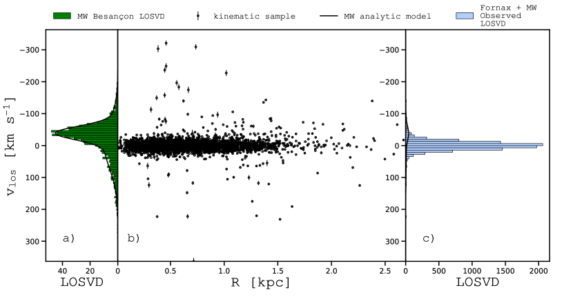
Figure 1: Panel a: The Milky Way’s LOSVD in the direction of Fornax calculated from the Besançon model (histogram) and the best-fitting two-Gaussian distribution (black line). The LOSVD of the Besançon model has been shifted by $v_{\rm sys}$ to make the comparison coherent. Panel b: position-velocity diagram of the whole kinematic sample used in this work (Fornax + MW; data taken from Battaglia et al. 2006 and Walker et al. 2009; see text). Panel c: Fornax + MW observed LOSVD superimposed to the best fitting two-Gaussian distribution of panel a. The observed total LOSVD (Fornax + MW) of panel c is normalized to the total number of stars (Fornax + MW) expected from the Battaglia et al. (2006) photometric sample, while the MW model of panels a and c is normalized to the total number of the field stars expected in the very same region according to the Besançon model. Note the very different scales of the x-axis of panels a and c.

Parameter	Value	Reference
RA	2h 39m 52s	1
DEC	-34°30’ 49”	1
P.A.	46.8°$\pm$1.6°	1
$\epsilon$	0.30$\pm$0.01	1
$d$ [kpc]	138	1
$R_{\rm e}$ [kpc]	0.62	1
$N_{n}$	27	1
$n_{\rm f}$ [stars arcmin-2]	0.263	1
$v_{\rm sys}\quad[\,{\rm km\,s}^{-1}]$	55.1	2
$N_{v}$	2990	3

Table 2: Values of the main observational parameters of Fornax used in this work: right ascension (RA), declination (DEC), Position Angle (P.A.), ellipticity ($\epsilon$), distance from the sun ($d$), projected half-light radius ($R_{\rm e}$), number of bins of the projected stellar number density profile ($N_{n}$), mean projected number density of the field stars ($n_{\rm f}$), systemic heliocentric velocity ($v_{\rm sys}$), number of members of the kinematic sample ($N_{v}$). References: 1) Battaglia et al. 2006, 2) Breddels & Helmi 2013, 3) this work.

Our photometric sample is taken from Battaglia et al. (2006), who, using deep ESO/WIFI observations, studied the spatial distribution of the stars of Fornax and derived its main structural parameters. Adopting a distance $d=138$ kpc (Battaglia et al. 2006), the projected stellar number density profile extends out to $3.33\,$kpc and it is composed of $N_{n}=27$ concentric elliptical shells of semi-major axis length $R_{i,{\rm ell}}$ of equal thickness, so $R_{i+1,{\rm ell}}-R_{i,{\rm ell}}=0.12\,$kpc for all $i$. The shells have ellipticity $\epsilon=0.3$ (Battaglia et al. 2006). We use the observed projected stellar number density profile as a function of the circularized radius $R_{i}\equiv R_{i,{\rm ell}}\sqrt{1-\epsilon}$ with $i=1,..,N_{n}$. The circularized projected half-light radius is $R_{\rm e}=0.62\,$kpc.

Family	$\alpha$	$\eta$	$\tilde{M}_{0,\rm dm}$	$\tilde{J}_{0,\rm dm}$	$\tilde{J}_{\rm c,dm}$	$\tilde{J}_{\rm t,dm}$	$J_{0,\star}$/[km s-1 kpc]	$M_{0,\star}$/[$M_{\odot}$]
FnxMFL	$1.52^{+0.03}_{-0.04}$	$0.49^{+0.02}_{-0.03}$	0	–	–	–	$6.87^{+0.28}_{-0.44}$	$7.70^{+0.76}_{-1.09}\times 10^{7}$
FnxNFW	$1.39^{+0.02}_{-0.03}$	$0.38^{+0.02}_{-0.02}$	$2.26^{+0.44}_{-0.41}\times 10^{2}$	$76.49^{+4.21}_{-3.85}$	–	6	$5.00^{+0.35}_{-0.28}$	$1.70^{+0.37}_{-0.27}\times 10^{7}$
FnxCore1	$0.84^{+0.02}_{-0.02}$	$0.49^{+0.03}_{-0.03}$	$1.56^{+0.28}_{-0.39}\times 10^{4}$	$196.58^{+15.43}_{-21.02}$	0.02	6	$2.19^{+0.27}_{-0.16}$	$5.52^{+1.81}_{-0.87}\times 10^{5}$
FnxCore2	$0.65^{+0.02}_{-0.02}$	$0.56^{+0.04}_{-0.03}$	$6.23^{+2.11}_{-2.14}\times 10^{4}$	$290.18^{+39.68}_{-40.34}$	0.20	6	$0.98^{+0.16}_{-0.12}$	$1.46^{+0.73}_{-0.38}\times 10^{5}$
FnxCore3 (Best Model)	$0.62^{+0.02}_{-0.01}$	$0.56^{+0.04}_{-0.02}$	$5.87^{+0.93}_{-2.22}\times 10^{4}$	$177.08^{+15.80}_{-29.59}$	0.67	6	$0.84^{+0.17}_{-0.07}$	$1.06^{+0.68}_{-0.10}\times 10^{5}$

Table 3: Input parameters of the best Fornax models of each family. $\alpha$ and $\eta$: parameters of the stellar DF (2). $\tilde{M}_{0,\rm dm}\equiv M_{0,\rm dm}/M_{0,\star}$. $\tilde{J}_{0,\rm dm}\equiv J_{0,\rm dm}/J_{0,\star}$. $\tilde{J}_{\rm c,dm}\equiv J_{\rm c,dm}/J_{0,\rm dm}$. $\tilde{J}_{\rm t,dm}\equiv J_{\rm t,dm}/J_{0,\rm dm}$. $J_{0,\star}$ and $M_{0,\star}$: respectively, action and mass scales (equation 2). $M_{0,\rm dm}$, $J_{0,\rm dm}$, $J_{\rm c,dm}$ and $J_{\rm t,dm}$ are the parameters of the dark-matter DF (equations 4-7). The best model is the FnxCore3.

Family	$\tilde{r}_{\rm c}$	$\tilde{M}_{\rm tot,dm}$	$M_{\rm tot,\star}$ $/[M_{\odot}]$	$(M_{\text{dm}}/M_{\star})|_{3{\rm kpc}}$	$\beta|_{1{\rm kpc}}$	$\ln\mathcal{L}_{\rm max}$	${\rm AIC}$	$\Delta{\rm AIC}$	$P$
FnxMFL	–	–	$2.06^{+0.13}_{-0.12}\times 10^{8}$	–	$-0.32^{+0.13}_{-0.16}$	-12605.88	25219.76	185.74	$4.65\times 10^{-41}$
FnxNFW	–	$63^{+14}_{-6}$	$9.23^{+0.77}_{-2.85}\times 10^{7}$	$2.6^{+2.3}_{-0.8}$	$-0.73^{+0.23}_{-0.29}$	-12582.16	25174.32	140.3	$3.4\times 10^{-31}$
FnxCore1	$0.425^{+0.001}_{-0.012}$	$1301^{+7}_{-164}$	$1.00^{+0.73}_{-0.00}\times 10^{7}$	$73^{+1}_{-33}$	$-0.17^{+0.15}_{-0.14}$	-12530.26	25070.52	36.5	$1.2\times 10^{-8}$
FnxCore2	$1.075^{+0.001}_{-0.053}$	$1344^{+38}_{-280}$	$1.03^{+1.37}_{-0.03}\times 10^{7}$	$125^{+5}_{-76}$	$0.07^{+0.12}_{-0.13}$	-12512.66	25035.32	1.3	0.52
FnxCore3 (Best Model)	$1.272^{-0.001}_{-0.035}$	$946^{+1}_{-213}$	$1.00^{+1.34}_{-0.00}\times 10^{7}$	$144^{+2}_{-87}$	$0.08^{+0.14}_{-0.12}$	-12512.01	25034.02	0	1

Table 4: Output parameters of the best Fornax models of each family. $\tilde{r}_{\rm c}$: ratio between the core radius of the dark matter and the half-mass radius of the stellar component. $\tilde{M}_{\rm tot,dm}\equiv\tilde{M}_{\rm tot,dm}/M_{\rm tot,\star}$. $M_{\rm tot,\star}$: stellar total mass. $(M_{\text{dm}}/M_{\star})|_{3{\rm kpc}}$: dark-matter to stellar mass ratio within 3 kpc. $\beta|_{1{\rm kpc}}$: anisotropy parameter (equation 39) measured at 1 kpc. $\ln\mathcal{L}_{\rm max}$: log-likelihood (equation 28). ${\rm AIC}$: value of the Akaike Information Criterion (equation 36). $\Delta$AIC: difference between the AIC of the best model of a family and the best of all models (FnxCore3). $P$: probability that a model represents the data as well as the best in any family (FnxCore3). All models have $\tilde{r}_{\rm s}=4$ and $r_{\rm h}\simeq 0.81\,$kpc.

Our reference kinematic sample of Fornax’s stars is taken from Battaglia et al. (2006) and Walker et al. (2009). This joined sample has already been used by Breddels & Helmi (2013), who corrected the line-of-sight velocities for the systemic velocity of Fornax $v_{\rm sys}$ and for the gradient due to the extent of Fornax on the sky (for details see Table 2 and Breddels & Helmi 2013). We apply the same corrections here. The samples have been cross-matched with an astrometric precision of 1 arcsec and, for each duplicate (i.e. stars with two measured velocities), being $\delta v_{1}$ and $\delta v_{2}$ the different velocity errors of the cross-matched stars, we compute the average error

$$\delta v=\sqrt{\frac{\delta v_{1}^{2}+\delta v_{2}^{2}}{2}}.$$ (38)

If the difference between the two velocities is larger than 3$\delta v$, we exclude the star from both the samples since we consider the difference to be caused by an unresolved binary. Otherwise, we use the mean of the two velocities. From the 945 stars of the Battaglia et al. (2006) sample and the 2633 of the Walker et al. (2009) sample, we find 488 cross-matched stars, 100 of which ($\approx$20%) we classify binaries and thus exclude. In this way, the final kinematic sample consists of 2990 stars, each of which characterised by its line-of-sight velocity $v_{{\rm los},k}$ and its circularised radius $R_{k}$ (equation 25).

Of course, our kinematic sample is still contaminated by undetected binaries. For instance, we expect to have in our sample about 600 undetected binaries ($\approx$20% of the non-cross matched stars) with properties similar to those excluded from the cross-matched sample. Therefore we must quantify the effect of binary contamination on the LOSVD of our spectroscopic sample of Fornax. The contamination from undetected binaries is problematic when the characteristic velocity of short-period binaries is comparable with the line-of-sight velocity dispersion. Minor et al. (2010) found that for dwarfs with mean line-of-sight velocity dispersion in the range $4\lesssim\sigma_{\rm los}$/km s^-1 $\lesssim 10$ the velocity dispersion profile may be inflated by no more than 15% by undetected binaries, so binaries should have a negligible effect on Fornax, which has $\sigma_{\rm los}\simeq 12$ km s^-1.

In principle, though negligibly affecting $\sigma_{\rm los}$, the binaries could have an impact on the observed LOSVD. We tried to quantify this effect as follows: we built two kinematic samples, one containing all the cross-matched stars (488 stars; sample A) and one containing only stars not classified as binaries according to the above criterion (388 stars; sample B). For these two samples we computed the LOSVD in two radial bins ($R<0.72$ kpc and $R>0.72$ kpc), such that each bin contains 244 stars in the case of sample A. According to the Kolmogorov-Smirnov test, in both radial bins the probability that the LOSVDs of samples A and B differ is less than 4%. This result indicates that the LOSVDs used in our analysis should not be biased by the presence of undetected binaries.

The fields of view in the direction of Fornax suffer from significant Galactic contamination: the mean velocity of MW stars in these fields is approximately the same as the systemic velocity of Fornax, which complicates the selection of a reliable sample of members. From Fig. 1b, showing the position-velocity diagram of our kinematic sample, and from Fig. 1a, showing the velocity distribution of the MW calculated from the Besançon model (Besanson2004) with a selection in magnitude comparable to the one of our kinematic sample ($18\lesssim V\lesssim 20.5$, with $V$ apparent $V$ band magnitude), we see that the LOSVDs of Fornax and MW stars overlap (see also Fig. 1c).

As explained in Section 3.1, we take into account contamination by the MW by adding to our models a component describing the LOSVD of MW stars in the direction of Fornax. The MW velocity distribution extracted from the Besançon model is fitted with a two-Gaussian distribution (Fig. 1a) which reflects the separate contributions of disc and halo stars. We assume a mean MW surface density $n_{\rm f}=0.263$ stars arcmin^-2, obtained from the Besançon model, applying the the same selection in the $V$-band apparent magnitude as in the kinematic sample ($18\lesssim V\lesssim 20.5$). A summary of the main observational parameters of Fornax used in this work is given in Table 2.

4.2 Results

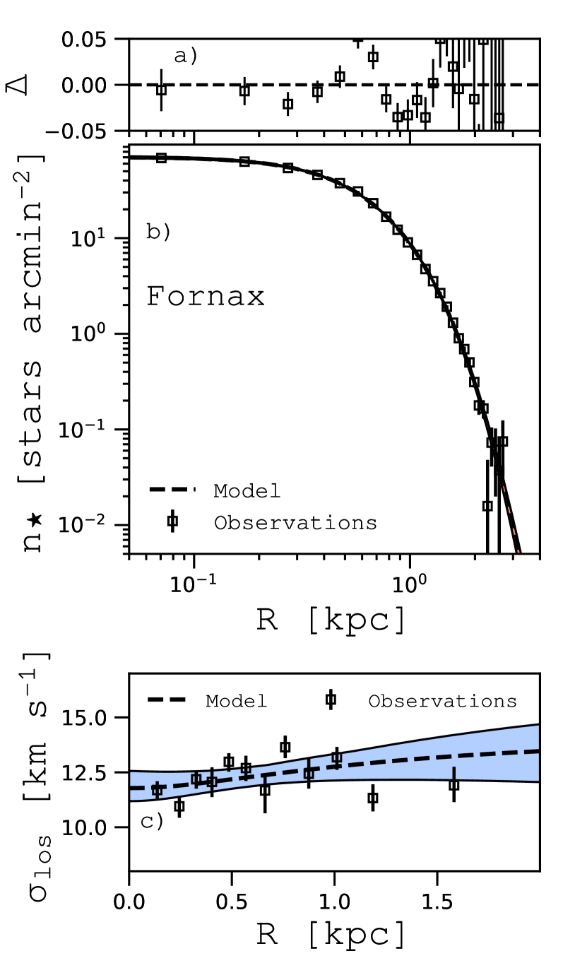
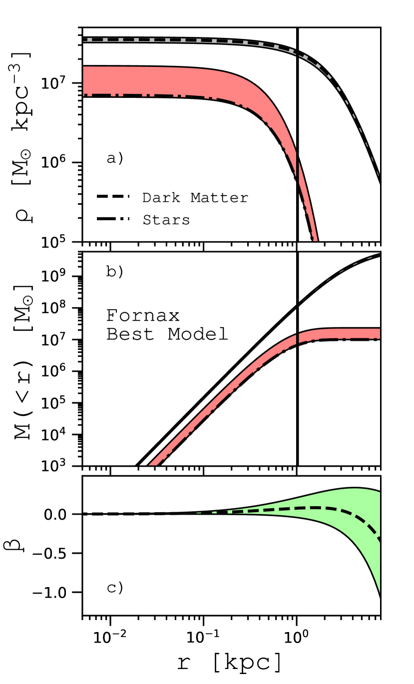
Figure 2: Panel a: residuals $\Delta=(n_{\star}^{\text{obs}}-n_{\star})/n_{\star}$ between the best model (FnxCore3) and the observed projected stellar number density profiles (dashed curve). Panel b: projected number density profile of the best model (dashed line) compared with the observed profile (points with error bars). Panel c: line-of-sight velocity dispersion profile of the best model compared with the observed profile (points with error bars). Bands show the 1$\sigma$ uncertainty (see Section 3.2). Note that the x-axis is logarithmic in panel b and linear in panel c.

Figure 3: Panel a: stellar (dash-dotted line) and dark-matter (dashed line) density profiles of the best model (FnxCore3) of Fornax. Panel b: stellar (dash-dotted line) and dark-matter (dashed line) mass profiles of the best model of Fornax. Panel c: stellar anisotropy parameter profile (dashed line) of the best model of Fornax. In panels a and b, the vertical lines mark the range of the halo core radius $r_{\rm s}$. The bands indicate the 1$\sigma$ uncertainty (see Section 3.2).

Here we present the results we obtained applying the $f(\bf J)$ models of Section 2 to the Fornax dSph. In particular we focus on two-component spherical models, in which the stars and the dark matter have different DFs. In Section 4.2.3 we will consider also simpler one-component spherical models, in which mass follows light. The physical properties of the models are computed by integrating equations (11), (12), (13), (26) and (27), using a code based on AGAMA (Action-based Galaxy Models Architecture, https://github.com/GalacticDynamics-Oxford/Agama; Vasiliev 2018), a software package that implements the action/angle formalism of $f({\bf J})$ DFs. To test the performances of our method, in the Appendix B we applied $f({\bf J})$ models to a mock galaxy with structural and kinematic properties similar to a typical dSph.

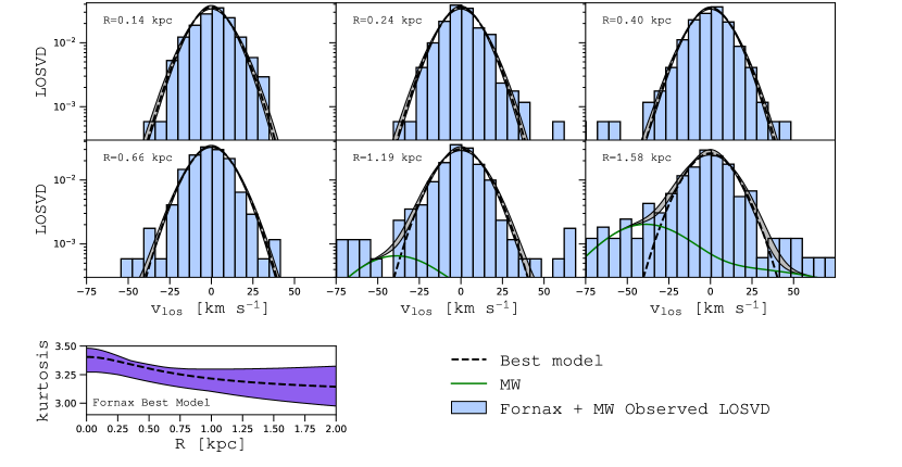
Figure 4: Observed Fornax + MW LOSVD (histograms) compared with the LOSVD of the best model (FnxCore3). In each panel, $R$ indicates the average radius of the radial bin where the LOSVD of the best model is computed. The radial bins are those used to construct the observed line-of-sight velocity dispersion profile of Fornax (Fig. 3). The green solid curve marks the MW’s contribution. The bottom panel shows the kurtosis profile of the best model’s LOSVD. The bands mark the 1$\sigma$ uncertainty (see Section 3.2).

In the two-component models of Fornax, we adopt four families of dark halos: a family with a cuspy NFW-like halo and three halo families with central cores. Outside the core region these fall off similarly to an NFW profile. For clarity, in the following we will refer to the cuspy NFW family as FnxNFW, and to the cored families as FnxCore$n$, with $n=1,2,3$, where higher $n$ indicate larger cores in the dark halo. The NFW halo is obtained setting $\tilde{J}_{\rm c,dm}=0$ in equation (6), while increasing values of $\tilde{J}_{\rm c,dm}$ produce cores of increasing sizes. The families FnxCore1, FnxCore2 and FnxCore3 have, respectively $\tilde{r}_{\rm c}\simeq 0.43,1.08,1.28$, corresponding to physical core radii $r_{\rm c}\simeq 0.34,0.87,1.03$ kpc (see Section 2.4). We recall that the circularised projected half-light radius of Fornax is $R_{\rm e}=0.62$ kpc (Section 4, Table 2). Based on observational estimates of the total stellar mass of Fornax (de Boer et al. 2012), we consider only two-component models such that $10^{7}\leq M_{\rm tot,\star}/M_{\odot}\leq 10^{8}$. We recall that the model $M_{\rm tot,\star}$ depends only on $\alpha$, $\eta$ and $M_{0,\star}$. Therefore, the above limits on $M_{\rm tot,\star}$ are in practice limits on $M_{0,\star}$, for given $\alpha$ and $\eta$. We fixed the ratio between the scale radius of the dark halo and the half-mass radius of the stellar component to $\tilde{r}_{\rm s}=4$, consistent with the values expected on the basis of the stellar-to-halo mass relation and the halo mass-concentration relation, for galaxies with stellar masses $10^{7}\leq M_{\rm tot,\star}/M_{\odot}\leq 10^{8}$ (see Section 4.2.4). We find that spherical models of Fornax have intrinsic stellar half-mass radius $r_{\rm h}\simeq 0.81$ kpc. It follows that our models have $r_{\rm s}=\tilde{r}_{\rm s}r_{\rm h}\simeq 3.3$ kpc. Under these assumptions, each family has 5 free parameters, ($\alpha$, $\eta$, $\tilde{M}_{\rm tot,dm}$, $J_{0,\star}$, $M_{0,\star})$. Tables 3 lists the values of the five parameters for the best model of each family, together with $\tilde{J}_{0,\rm dm}$ (fixed by the condition $\tilde{r}_{\rm s}=4$), $\tilde{J}_{\rm c,dm}$ (fixed for each family) and $\tilde{J}_{\rm t,dm}=6$ for all families. The choice of $\tilde{J}_{\rm t,dm}=6$ ensures, for all the families, that the truncation radius of the dark halo $\tilde{r}_{\rm t}$ is much larger than the scale radius $\tilde{r}_{\rm s}$. Table 4 gives some output parameters of the best Fornax model of each family.

4.2.1 Properties of the best model

According to our MLE (Section 3), the best model belongs to the FnxCore3 family, with the most extended core in the dark-matter density profile ($r_{\rm c}\simeq 1.03\,$kpc). In general, we find that a model in any cored families is strongly preferred to a NFW halo: the AICs (see Table 4) indicate that the introduction of even a small core in the dark-matter profile vastly improves the fit to the Fornax data.

Fig. 3b plots the projected stellar number density profile of the best model compared to the observed profile. The residuals between data and model are shown in Fig. 3a. Fig. 3c shows the line-of-sight velocity dispersion profile of the best model compared to the observed radially-binned profile. We followed Pryor & Meylan (1993) to compute the observed line-of-sight velocity dispersion profile, grouping the kinematic sample in 12 different radial bins, each containing 250 stars, except for the last bin which has 140 stars. In the calculation of the observed line-of-sight velocity profile we accounted for contamination by field stars as in equation (32), using the same MW Besançon model as in Section 4.1. The projected stellar number density profile is extremely well reproduced by our best model. A measure of the goodness of the fit to the projected surface density is given by the term $\ln\mathcal{L}_{n}$ of equation (28): for the best model $\ln\mathcal{L}_{n}\simeq-30$. For comparison, for the best-fitting Sersic (1968) profile of Fornax (Battaglia et al. 2006), $\ln\mathcal{L}_{n}\simeq-62.79$. Even accounting for the different numbers of free parameters as in equation (36), our model gives a better description of the projected number density than the Sérsic fit. This feature shows that our stellar DF is extremely flexible and well suited to describe the structural properties of dSphs. Our best model has a line-of-sight velocity dispersion profile slightly increasing with radius, which provides a good description of the observed profile. However, we recall that in the determination of the best model we do not consider the binned line-of-sight velocity dispersion profile, but compare individual star data with model LOSVDs, so to fully exploit the available data.

Fig. 3 plots the stellar and dark-matter density distributions, the stellar and dark-matter mass profiles, and the stellar anisotropy parameter profile of the best FnxCore3 model. The anisotropy parameter is

$$\beta=1-\frac{\sigma_{t}^{2}}{2\sigma_{r}^{2}},$$ (39)

where $\sigma_{r}$ and $\sigma_{t}$ are, respectively, the radial and tangential components of the velocity dispersion ($\sigma^{2}_{t}=\sigma^{2}_{\theta}+\sigma^{2}_{\phi}$, where $\sigma_{\theta}$ and $\sigma_{\phi}$ are angular components of the velocity dispersion in spherical coordinates; equation 13). Models are isotropic when $\beta=0$, tangentially biased when $\beta<0$ and radially biased when $0<\beta\leq 1$. The best model predicts Fornax to have slightly radially anisotropic velocity distribution: for instance, at $r=1\,$kpc the anisotropy parameter is $\beta|_{1{\rm kpc}}=0.08^{+0.14}_{-0.12}$ (see Fig. 3c). In our best model, the dark matter dominates the stellar component at all radii. The dark-matter to stellar mass ratio is $(M_{\text{dm}}/M_{\star})|_{R_{\rm e}}=9.6^{+0.6}_{-5.7}$ within $R_{\rm e}$ and $(M_{\text{dm}}/M_{\star})|_{3{\rm kpc}}=144^{+2}_{-87}$ within 3 kpc. The best model has a total stellar mass $M_{\rm tot,\star}=10^{7}M_{\odot}$, which is the lower limit imposed to the stellar mass on the basis of observational estimates (see Section  4.2).

Fig. 4 compares the observed LOSVD with the LOSVD of the best model. For this figure the observed LOSVD was computed in the same radial bins as the line-of-sight velocity dispersion profile of Fig. 3c, while the model LOSVD is evaluated at the average radius of each bin: for clarity, we show only 6 of the 12 radial bins, covering the whole radial extent of the kinematic sample. The best model has a sharply peaked LOSVD, indicative of radially biased velocity distribution, consistent with the observed LOSVD. The contamination from MW field stars grows with distance from the galaxy’s centre and is clearly visible in the outermost bin. The shape of the LOSVD can be quantified by the kurtosis

$$y(R)\equiv\frac{\int_{-\infty}^{+\infty}{\mathscr{L}}_{\star}(R,v_{||})(v_{||}-\bar{v})^{4}\text{d}v_{||}}{\left[\int_{-\infty}^{\infty}{\mathscr{L}}_{\star}(R,v_{||})(v_{||}-\bar{v})^{2}\text{d}v_{||}\right]^{2}},$$ (40)

which is the fourth centred moment of the LOSVD. The bottom panel of Fig 4 plots the kurtosis of the LOSVD of the best model as a function of the distance from the centre. The best model has a kurtosis which is constantly greater than $y=3$ (the kurtosis of a Gaussian distribution), which is a signature of peaked LOSVD and radial bias.

As is well known, dSphs are good candidates for indirect detection of dark-matter particles. The $\gamma$-ray flux due to dark-matter annihilation and decay depend on the dark-matter distribution through, respectively, the so called $J$ and $D$-factors. For sufficiently distant, spherically symmetric targets, it can be shown that the $J$-factor reduces to the integral

$$J(\theta)=\frac{2\pi}{d^{2}}\int_{-\infty}^{+\infty}\text{d}z\int_{0}^{\theta d}\rho_{\rm dm}^{2}R\text{d}R,$$ (41)

while the D-factor to

$$D(\theta)=\frac{2\pi}{d^{2}}\int_{-\infty}^{+\infty}\text{d}z\int_{0}^{\theta d}\rho_{\rm dm}R\text{d}R,$$ (42)

where $\theta=R/d$ is the angular distance from the centre of the galaxy, $z$ is the line-of-sight and $d$ is the distance of the galaxy (Table 2).  Fig. 5 plots the $J$-factor (panel a) and $D$-factor (panel b) as functions of the angular distance $\theta$ computed for our best model of Fornax. We measure at an angular distance $\theta=0.5^{\circ}$ (corresponding approximately to the angular resolution of the Fermi-LAT telescope in the GeV range)

$$\log_{10}(J\text{ }[\text{GeV}^{2}\text{cm}^{-5}])=18.34^{+0.06}_{-0.09}$$ (43)

and

$$\log_{10}(D\text{ }[\text{GeV cm}^{-2}])=18.55^{+0.03}_{-0.05},$$ (44)

consistent with Evans et al. (2016).

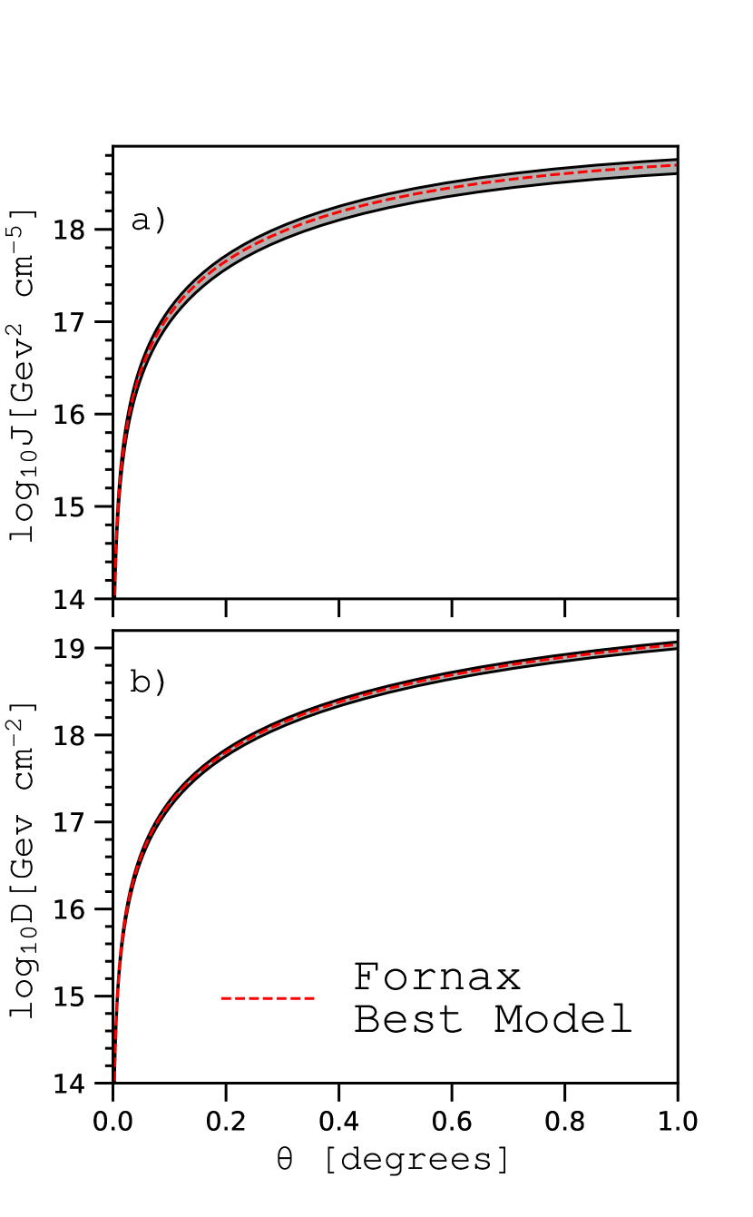
Figure 5: Panel a: dark-matter annihilation $J$-factor (equation 41) of the best model of Fornax (FnxCore3, dashed line) as function of the angular distance from the centre. Panel b: same as panel a, but for the dark-matter decay $D$-factor (equation 42). Bands mark the $1\sigma$ uncertainty (see Section 3.2).

4.2.2 Performances of other families of two-component models

Figure 6: Columns, from left to right, refer to the best models of the FnxNFW, FnxCore1, FnxCore2 and FnxMFL families, respectively. Top row of panels (a): residuals between the model and the observed projected stellar density profile (points with error bars). Residuals are defined as $\Delta\equiv(n_{\star}^{\text{obs}}-n_{\star})/n_{\star}$. Middle row of panels (b): projected number density profile of the model (dashed lines), compared with the observed profile (points with error bars). Bottom row of panels (c): line-of-sight velocity dispersion profile of the model (dashed lines), compared with the observed profile (points with error bars). In panels b and c the bands indicate the 1$\sigma$ uncertainties (see Section 3.2). In panel c the red curve shows the line-of-sight velocity dispersion of the best model of any family (FnxCore3). $r_{\rm c}$ is the size of the core radius, $r_{\rm h}$ is the stellar half-mass radius and $P$ is the probability of the model compared to FnxCore3 (equation 37).

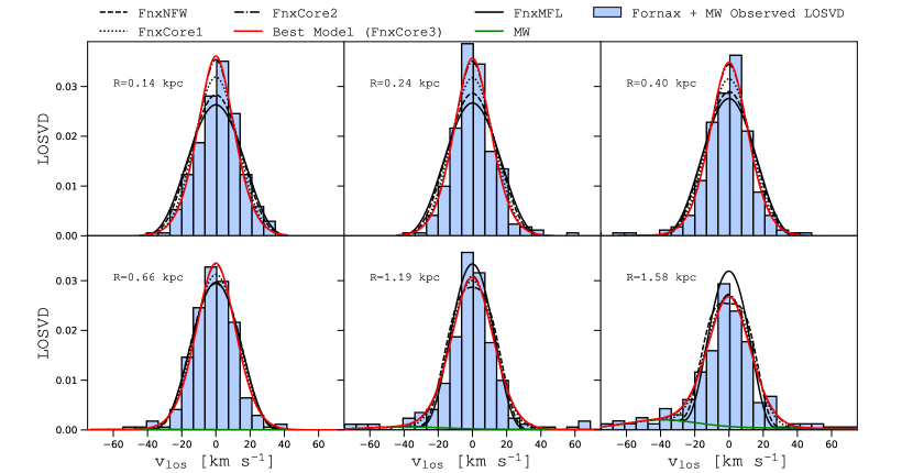
Figure 7: Comparison of the observed Fornax + MW LOSVD (histograms) and the LOSVDs of the best models in the families FnxNFW, FnxCore1, FnxCore2, FnxCore3 and FnxMFL (respectively dashed, dotted, dot-dashed, red solid and black solid curves). The overall best model is FnxCore3. In each panel, $R$ indicates the average radius of the radial bin for which data are shown, which is also the radius at which the model LOSVD was computed. The radial bins are the same as in Figs. 4 and 6c. The green curve marks the MW’s contribution.

Figure 8: Kurtosis profile of the LOSVD for the best models of the families FnxNFW, FnxCore1, FnxCore2, FnxMFL (dashed, dotted, dot-dashed, solid, respectively). The red curve without a band shows the kurtosis profile of the best of all models (FnxCore3). The bands show the 1$\sigma$ uncertainties (see Section 3.2).

Here we compare the best model of Section 4.2.1 with other families of two-component models of Fornax. The projected number density profiles of the best models of the FnxNFW, FnxCore1, FnxCore2 families and the observed Fornax surface density profile, and the residuals between models and data are plotted in Fig.s 6b and 6a. Fig. 6c shows the comparison with the line-of-sight velocity dispersion profiles. The projected number density profile is also well described by the other families, which have $-40\lesssim\ln\mathcal{L}_{n}\lesssim-25$, substantially better than the best-fitting Sérsic model. Among our models, those with cored halo reproduce well the flat behavior of the line-of-sight velocity dispersion profile, while the best FnxNFW predicts a slightly decreasing profile, which poorly represents the available data.

Fig. 7 shows the observed LOSVD compared to the model LOSVDs. The observed LOSVD is computed in the same radial bins as in Fig. 4. The LOSVD of FnxNFW is systematically more flat-topped than that observed or the LOSVDs of cored models, and, in the outermost bin, it has a double-peaked shape, indicative of tangential bias. In contrast, the more extended the core of a dark-matter density distribution, the more sharp-peaked the LOSVD is, and the more satisfying a description of the observed LOSVD it provides (Fig. 7). A quantitative measure of the shapes of a LOSVD is the kurtosis, which is plotted as a function of radius in Fig. 8. The best model of the FnxNFW family has a kurtosis which is everywhere much less than $y=3$, while the cored families with the most extended cores have $y>3$. In other words, a model with NFW halo cannot reproduce at same time the flat line-of-sight velocity dispersion profile and the peaked LOSVD observed in Fornax.

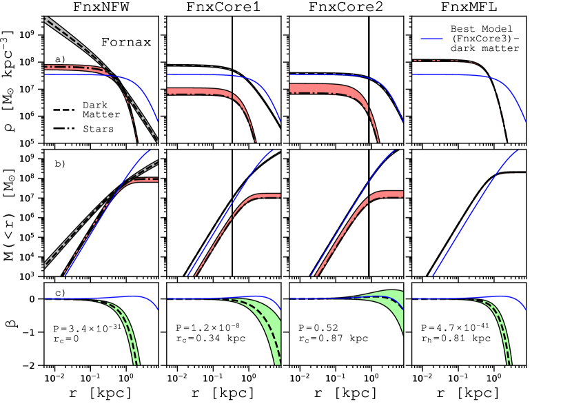
Figure 9: Columns, from left to right, refer to the best model of the FnxNFW, FnxCore1, FnxCore2 and FnxMFL families, respectively. Top row of panels (a): stellar (dash-dotted line) and dark-matter (dashed line) density profiles. Middle row of panels (b): stellar (dash-dotted line) and dark-matter (dashed line) mass profiles. Bottom row of panels (c): anisotropy parameter profile (dashed line). The vertical black lines in the four top and middle panels mark the dark halo’s core radius $r_{\rm c}$. In all panels the bands around the best fits indicate 1$\sigma$ uncertainty (see Section 3.2). The blue curve marks the dark-matter density (panels a), dark-matter mass (panels b) and stellar anisotropy profiles (panels c) of the best of all models (FnxCore3). $r_{\rm h}$ is is the stellar half-mass radius and $P$ is the probability of the model compared to the best of all models (FnxCore3).

Figs. 9a and 9b plot the stellar and dark matter density and mass profiles, respectively. The best models of all families with cored halos have a total stellar mass of $10^{7}M_{\odot}$, while the best NFW model has a total stellar mass of $9.23^{+0.77}_{-2.85}\times 10^{7}$ $M_{\odot}$. Stars never dominate over the dark matter in the case of cored halos, where $(M_{\text{dm}}/M_{\star})|_{R_{\rm e}}=13.4^{+0.1}_{-5.8}$ and $9.7^{+0.4}_{-5.7}$, respectively, for the FnxCore1 and FnxCore2 cases, whereas they do in the cuspy halo one, where $(M_{\text{dm}}/M_{\star})|_{R_{\rm e}}=1.12^{+0.86}_{-0.32}$. We also find a slight trend of the core size to be larger when the dynamical-to-stellar mass ratios are smaller.

Fig. 9c plots the profile of the stellar anisotropy parameter for the best model in each family. It shows that the anisotropy varies with the size of the core: the more extended the core, the more radially biased the galaxy. Indeed, the NFW halo requires a highly-tangentially biased system ($\beta|_{1{\rm kpc}}=-0.73^{+0.23}_{-0.29}$), the FnxCore1 model requires isotropic to slightly tangential bias, while the best model, with the most extended core, has a preference for radial orbits (Fig.s 4, 7 and 8, Table 4).

By comparing the AICs (Table 4), we note that, while the best model FnxCore2 is comparable to the best model (FnxCore3), with probability $P=0.52$ (equation 37), the FnxCore3 model is significantly preferable to both a model with a NFW dark halo and a model with a small core in the dark-matter density distribution. For the FnxNFW, $\Delta$AIC$=140.3$, while for the FnxCore1 $\Delta$AIC$=36.5$, values that translate in extremely small probabilities $P$ ($P\simeq 3.4\times 10^{-31}$ and $P\simeq 10^{-8}$, respectively). We pointed out that different families are almost equivalent in describing the projected number density profile, so we can safely state that most of the differences that allow us to discriminate between cored and cuspy models are attributable to our kinematic analysis, which minimises any loss of information (e.g. self-consistent LOSVD, no binning).

The best Fornax model belongs to the family with the largest core among those considered so far, so it is worth asking if the data allow us to put an upper limit on the dark-matter core radius $\tilde{r}_{\rm c}$. To do that, we run two additional experiments, considering families with core radii, respectively, $\tilde{r}_{\rm c}\simeq 2.4$ ($r_{\rm c}\simeq 1.94$ kpc) and $\tilde{r}_{\rm c}\simeq 4.8$ ($r_{\rm c}\simeq 3.89$ kpc). We find that these families have, respectively, $\ln\mathcal{L}_{\rm max}=-12513.4$ and $\ln\mathcal{L}_{\rm max}=-12514.8$, and probabilities (equation 37) $P=0.25$ and $P=0.06$, relative to the best of all models ($r_{\rm c}\simeq 1.03$ kpc). The results of these experiment suggest that the core of Fornax dark halo is smaller than the truncation radius ($\approx$ 2 kpc; see Section 4.2.4) of the stellar distribution.

4.2.3 Performance of one-component models

Given that in the best two-component model (FnxCore3) the central slopes of the stellar and dark-matter distributions are similar (Fig. 3), it is worth exploring also a simpler one-component family of $f({\bf J})$ models. In particular, here we consider the case in which the only component has the DF given by equation (2). This family of models can be interpreted as describing a system without dark matter, but also as mass-follows-light (MFL) models, in which dark matter and stars have the same distribution. We will refer to this family of models as FnxMFL. Since in this case $M_{0,\rm dm}=0$, this family has four free parameters ($\alpha$, $\eta$, $J_{0,\star}$, $M_{0,\star}$; equation 2). In Tab. 3 we report the parameters corresponding to the best FnxMFL model. The right column of Fig. 6 plots the projected number density profile and the line-of-sight velocity profile of the best FnxMFL model. The projected number density profile is well reproduced also by the MFL models, for which $\ln\mathcal{L}_{n}\simeq-40$, still much better than a Sérsic fit, while the line-of-sight velocity dispersion profile is clearly far from giving a good description of the observed profile. Fornax MFL models are rejected with high significance: we find $\Delta$AIC$=185.74$, the largest $\Delta$AIC among our models, consequently, with a probability $P\simeq 10^{-41}$.

In Fig. 7 the LOSVD of the FnxMFL model is compared with the LOSVD of the two-component models. MFL models tend to underestimate the observed LOSVD in the innermost regions (top three panels) and to overestimate it in the outermost regions (bottom three panels).

The rightmost column of Fig. 9 plots in panels a, b and c, respectively, the density, mass and anisotropy parameter profile predicted by the best FnxMFL model, which has total mass $M_{\rm tot,\star}=2.06^{+0.13}_{-0.12}\times 10^{8}$ $M_{\odot}$. Under the assumption that the dark halo follows the density distribution of the stellar component, this value is an indication of the dynamical (stellar plus dark-matter) mass. The FnxMFL model is tangentially anisotropic with $\beta|_{1{\rm kpc}}=-0.32^{+0.13}_{-0.16}$. The main parameters of this model are summarised in Tables 3 and 4.

4.2.4 Insensitivity to the halo scale radius

All the two-component models considered above have the scale radius of the dark halo fixed to $\tilde{r}_{\rm s}=4$. In this Section we relax this assumption and let $\tilde{r}_{\rm s}$ vary. Of course we are interested only in exploring cosmologically motivated values of $\tilde{r}_{\rm s}$, which can be evaluated as follows. According to current estimates of the low-mass end of the stellar-to-halo mass relation (Read et al. 2017), galaxies with stellar mass $M_{\rm tot,\star}=10^{7}-10^{8}$ $M_{\odot}$ (such as Fornax) have virial mass $4.5\times 10^{9}\lesssim M_{200}\lesssim 3\times 10^{10}$ $M_{\odot}$ and virial radius $35\lesssim r_{200}/$kpc $\lesssim 61$. According to the halo mass-concentration relation (Muñoz-Cuartas et al. 2011), in the present-day Universe halos in this mass range have $14\lesssim r_{200}/r_{\rm s}\lesssim 16$, so $2\lesssim r_{\rm s}/$kpc$\lesssim 5$, or $2.5\lesssim\tilde{r}_{\rm s}\lesssim 6.2$, for $r_{\rm h}\simeq 0.81$ kpc, which is the stellar half-mass radius of Fornax.

Even the lower bound of this cosmologically motivated interval of values of the scale radius ($r_{\rm s}\simeq 2$ kpc) is beyond the truncation of the stellar component of Fornax (97% of the stellar mass is contained within 2 kpc; see Fig.s 3b and 9b), so we do expect our results to be insensitive to the exact value of $r_{\rm s}$ within the above range. However, given the very poor performance of the NFW models in reproducing the observed kinematics of Fornax (Section 4.2.2), we explored also a more general family of NFW models, named FnxNFW-rs, in which $\tilde{r}_{\rm s}$ is a free parameter, in the range $2.5-6.2$. As predicted, these models turned out to be poorly sensitive to $r_{\rm s}$, with a slight preference for higher values. The best model of this new NFW family has $\tilde{r}_{\rm s}=6.04^{+0.16}_{-3.52}$, so all the explored values of $\tilde{r}_{\rm s}$ are within $1\sigma$. This model has $\ln\mathcal{L}=-12581.14$ and AIC$=25174.28$ (see Table 5), which, compared to the best model (FnxCore3), gives $\Delta$AIC$\sim 140.26$, approximately the same $\Delta$AIC as the best model of the family FnxNFW (Section 4.2.2). We conclude that the results obtained fixing $\tilde{r}_{\rm s}$ are robust against uncertainties on this parameter.

Family	$\alpha$	$\eta$	$\tilde{M}_{0,\rm dm}$	$\tilde{J}_{0,\rm dm}$	$J_{0,\star}$/[km s-1 kpc]	$M_{0,\star}$/[$M_{\odot}$]
FnxNFW-rs	$1.36^{+0.03}_{-0.04}$	$0.37^{+0.03}_{-0.02}$	$439^{+87}_{-182}$	$100.95^{+7.10}_{-11.25}$	$4.75^{+0.46}_{-0.30}$	$1.30^{+0.66}_{-0.17}\times 10^{7}$
	$\tilde{r}_{\rm s}$	$\tilde{M}_{\rm tot,dm}$	$\ln\mathcal{L}_{\rm max}$	${\rm AIC}$	$\Delta$AIC	$P$
FnxNFW-rs	$6.04^{+0.16}_{-3.52}$	$110.9^{+19.5}_{-34.9}$	-12581.14081	25174.28	140.25	$3.5\times 10^{-31}$

Table 5: Parameters of the best Fornax model of the FnxNFW-rs family with free scale radius (Section 4.2.4). $\alpha$ and $\eta$: parameters of the stellar DF (2). $\tilde{M}_{0,\rm dm}\equiv M_{0,\rm dm}/M_{0,\star}$. $\tilde{J}_{0,\rm dm}\equiv J_{0,\rm dm}/J_{0,\star}$. $J_{0,\star}$ and $M_{0,\star}$: respectively, action and mass scales (equation 2). $\tilde{M}_{\rm tot,dm}\equiv\tilde{M}_{\rm tot,dm}/M_{\rm tot,\star}$. As in the family FnxNFW (Table 3) $\tilde{J}_{\rm c,dm}\equiv J_{\rm c,dm}/J_{0,\rm dm}=0$ and $\tilde{J}_{\rm t,dm}\equiv J_{\rm t,dm}/J_{0,\rm dm}=6$. $M_{0,\rm dm}$, $J_{0,\rm dm}$, $J_{\rm c,dm}$ and $J_{\rm t,dm}$ are the parameters of the dark-matter DF (equations 4-7). $\tilde{r}_{\rm s}\equiv r_{\rm s}/r_{\rm h}$. $\tilde{M}_{\rm tot,dm}\equiv M_{\rm tot,dm}/M_{\rm tot,\star}$. $r_{\rm s}$ and $r_{\rm h}$ are, respectively the halo scale radius and the half-mass radius of the stellar component; $M_{\rm tot,dm}$ and $M_{\rm tot,\star}$ are, respectively, the total dark-matter and stellar masses (equations 10 and 9). $\ln\mathcal{L}_{\rm max}$: log-likelihood (equation 28). ${\rm AIC}$: value of the Akaike Information Criterion (equation 36). $\Delta$AIC: difference between the AIC of the FnxNFW-rs and the best of all models (FnxCore3, see Table 4). $P$: probability that the FnxNFW-rs best model represents the data as well as the best of all models (FnxCore3).

4.3 Comparison with previous work

Figure 10: Total mass profiles (stars and dark matter) of the FnxNFW, FnxCore1, FnxCore2, FnxCore3 and FnxMFL families. The bands mark the 1$\sigma$ uncertainty (see Section 3.2). The vertical red-dashed line indicates $r_{\rm m}$, radius where the total mass is model-independent.

Here we compare the results of our dynamical modelling of Fornax with previous works. Fig. 10 plots the dynamical (stars plus dark matter) mass profile of the best of our models (FnxCore3) compared to those of the best models of other families. Within the radius $r_{\rm m}\simeq 1.7$ $R_{\rm e}$ $\simeq 1.05$ kpc, the dynamical mass is robustly constrained against changes in the specific shape of the dark halo and the anisotropy. In our best model, the total mass enclosed within $r_{\rm m}$ is $M_{\rm dyn}(r_{\rm m})=1.38^{+0.10}_{-0.10}\times 10^{8}M_{\odot}$, consistent with the mass estimate of Amorisco & Evans (2011) of $M_{\rm dyn}(1.7$ $R_{\rm e})\simeq 1.3\times 10^{8}$ $M_{\odot}$. Amorisco & Evans (2011) performed a dynamical study of 28 dSphs, using different halos and modelling the stellar component with an ergodic King DF (Michie 1963, King 1966). Remarkably, they find that, for all the dSphs in their sample, the best mass constraint is given at $r_{\rm m}\simeq 1.7$ $R_{\rm e}$.

Strigari et al. (2008) performed a Jeans analysis on a sample of 18 dSphs. They used analytical density distributions for the dark matter in order to describe both cuspy and cored models, and studied the cases of anisotropic stellar velocity distributions, with radially varying anisotropy. They use a maximum likelihood criterion based on individual star velocities, assuming Gaussian LOSVDs. For all the dSphs, the authors find that $M_{\rm dyn}(300$ pc$)$, the total mass within 300 pc, is well constrained, and they estimate for Fornax $M_{\rm dyn}(300$ pc$)=1.14^{+0.09}_{-0.12}\times 10^{7}$ $M_{\odot}$, For our best model we find a smaller value, $M_{\rm dyn}(300$ pc$)=0.44^{+0.07}_{-0.03}\times 10^{7}$ $M_{\odot}$.

Walker et al. (2009) performed a Jeans analysis on a wide sample of dSphs finding that a robust mass constraint is given at $R_{\rm e}$, where, for the Fornax dSph, they measure $M_{\rm dyn}(R_{\rm e})=4.3^{+0.6}_{-0.7}\times 10^{7}$ $M_{\odot}$, marginally consistent with $M_{\rm dyn}(R_{\rm e})=3.37^{+0.33}_{-0.22}\times 10^{7}$ $M_{\odot}$, that we get for our best model.

The existence of a particular radius where the total mass is tightly constrained over a wide range of dark halo density profiles and anisotropy has been noted by many authors (Peñarrubia et al. 2008, Strigari et al. 2008, Walker et al. 2009, Wolf et al. 2010). However, there is not always agreement on the value of this particular radius, so it is worth asking why these differences arise. Dynamical modelling faces the problem that since one has to deal with only a 3D projection of the six-dimensional phase space (two coordinates in the plane of the sky and the line-of-sight velocities), the DF is not fully constrained by observations. Jeans analysis provides a work-around: the Jeans equations predict relations between some observables without delivering the DF and they do not require significant computational effort. However, Jeans analysis is not conclusive, because it is not guaranteed that the resulting model is physical in the sense that it has an everywhere non-negative DF (e.g. Ciotti & Morganti 2010, Amorisco & Evans 2011). Moreover, it involves differentiation of the data and does not deliver the LOSVD but only its first two moments. By contrast, the non-negativity of all our DFs is guaranteed, our procedure does not entail differentiation of the data, and we can exploit all the information that is contained in the LOSVD. It is reassuring that our estimate of $M_{\rm dyn}(1.7R_{\rm e})$ is consistent with Amorisco & Evans (2011), which is, to our knowledge, the only other work in which Fornax is modeled starting from DFs.

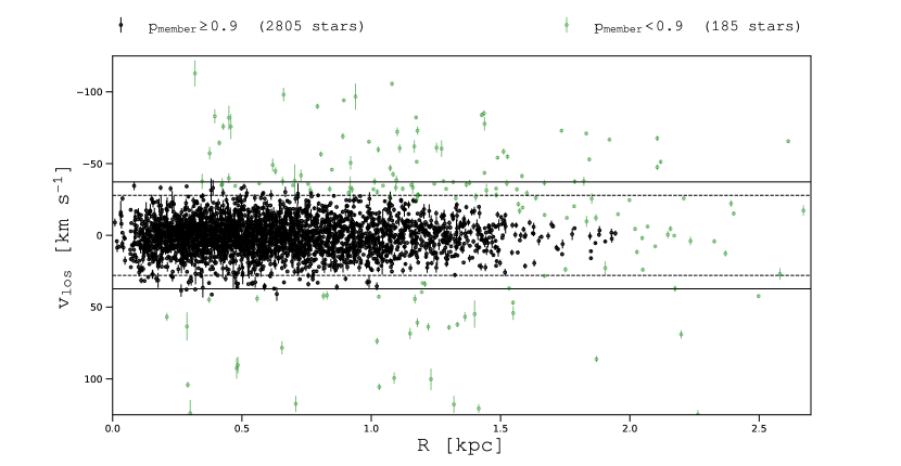
Figure 11: Position-velocity diagram of the Fornax kinematic sample. Different colours mark different membership probabilities $p_{\rm member}$; the horizontal dashed and solid lines mark the regions obtained by using an iterative $2.5\sigma$-clip and $3\sigma$-clip, respectively.

Recently, Diakogiannis et al. (2017) presented a new, spherical, non-parametric Jeans mass modelling method, based on the approximation of the radial and tangential components of the velocity dispersion tensor via $B$-splines and applied it to the Fornax dSph. Even considering different cases of dark-matter density distributions, they find that the best Fornax model is a simple MFL model. In our case, the MFL scenario is rejected with high significance (see Table 4). The authors measure a total mass of $M_{\rm dyn}=1.613^{+0.050}_{-0.075}\times 10^{8}$ $M_{\odot}$, which is slightly smaller than the total mass of our MFL models, $2.06^{+0.13}_{-0.12}\times 10^{8}$ (see Section 4.2.3). The best model of Diakogiannis et al. (2017) is characterised by tangential anisotropy, with mean anisotropy $\langle\beta\rangle=-0.95^{+0.78}_{-0.72}$, in agreement with the values we obtain from our FnxMFL models, which predict Fornax to be tangentially biased, with a reference anisotropy $\beta|_{1{\rm kpc}}=-0.32^{+0.13}_{-0.16}$. There are several differences between our analysis and that of Diakogiannis et al. (2017) that together explain the different conclusions about MFL models of Fornax. We believe that our model-data comparison is more accurate in some respects, which makes our conclusions more robust. For instance, we use a more extended observed stellar surface density profile and we account self-consistently for the MW contamination.

Breddels & Helmi (2013) applied spherical Schwarzschild (1979) modelling to four of the classical dSphs, including Fornax, assuming NFW, cored and Einasto (1965) dark-matter density profiles. They use both the second and the fourth moment of the LOSVD in comparisons with data. They conclude that models with cored and cuspy halo yield comparable fits to the data, and they find that models conspire to constrain the total mass within $1\,$kpc to a value $M_{\rm dyn}(1$ kpc$)\simeq 10^{8}$ $M_{\odot}$ that is in good agreement with our value, $M_{\rm dyn}(1$ kpc$)=1.20^{+0.09}_{-0.08}\times 10^{8}$ (Fig. 10). Breddels & Helmi (2013) find that the data for Fornax are consistent with an almost constant, isotropic or slightly tangential-biased anisotropy parameter profile $\beta=-0.2\pm 0.2$, marginally consistent with our almost isotropic values.

As far as the central dark-matter distribution is concerned, our results confirm and strengthen previous indications that Fornax has a cored dark halo. For instance, Goerdt et al. (2006) argue that the existence of five globular clusters in Fornax is inconsistent with the hypothesis of a cuspy halo since, due to dynamical friction, the globular clusters would have sunk into the centre of Fornax in a relatively short time (see also Sánchez-Salcedo et al. 2006, Arca-Sedda & Capuzzo-Dolcetta 2016). Amorisco et al. (2013), exploiting the information on the spatial and velocity distributions of Fornax subpopulations of stars, showed that a cored dark halo represents the data better and were able to constrain the size of the core, finding $r_{\rm c}=1^{+0.8}_{-0.4}\,$kpc, which agrees with the size of the core of our best model. Jardel & Gebhardt (2012) applied Schwarzschild axisymmetric mass models to Fornax, testing NFW and cored models with and without a central black hole. They used the LOSVD computed in radial bins to constrain the models, finding that the best model has a cored dark halo. They also computed the anisotropy profile according to their best model selection and argue that Fornax has a slightly radially biased orbit distribution, in agreement with our estimate. Walker & Peñarrubia (2011), considering two different stellar subpopulations of Fornax, provided anisotropy-independent estimates of the enclosed mass within 560 pc and 900 pc, $M(560$ pc$)=3.2\times 10^{7}M_{\odot}$ and $M(900$ pc$)=11.1\times 10^{7}M_{\odot}$, which are in perfect agreement with our results (Fig. 10).

4.4 Membership

As a further application of our DF-based method, we computed the probability that each star of the kinematic sample of Fornax is a member of the dSph. Contaminants are objects that, due to projection effects, seem to belong to an astrophysical target, but that are intrinsically located in foreground or background. Separating member stars from foreground contaminants is not an easy task, especially when they have similar magnitudes, colours, metalliticies, or when foreground stars move at similar velocities with respect to the target’s systemic velocity: this is, in particular, the case for Fornax. This makes usual approaches, such as the $n\sigma$-clip of the line-of-sight velocity of stars, ineffective. The $n\sigma$-clip strongly depends on the choice of the threshold $n$ and, in cases such as that of Fornax, it does not ensure the reliable exclusion of contaminants. Thus, we use an alternative approach to define a posteriori membership probabilities that relies on the LOSVD of our best model and of the Besançon model of the foreground.

We define $p_{\rm member}$ the probability that a star belongs to a certain target (in our case Fornax) and $p_{\rm cont}\equiv 1-p_{\rm member}$ the probability that the stars belongs to the contaminants population. In general

$$p_{\rm member}\equiv p_{\rm member}({\boldsymbol{\theta}}),$$ (45)

where ${\boldsymbol{\theta}}$ describes some measured properties of the stars. Let us focus on the simple case in which ${\boldsymbol{\theta}}=(R,v_{\rm los})$ and define the membership probability of the $k$-th star as

$$p_{{\rm member},k}=\frac{(1-\omega_{k})\int_{-\infty}^{+\infty}\mathcal{L}_{\star}(R_{k},v_{||})G_{k}(v_{||}-v_{{\rm los},k})\text{d}v_{||}}{\int_{-\infty}^{+\infty}\mathcal{L}_{\rm tot}(R_{k},v_{||})G_{k}(v_{||}-v_{{\rm los},k})\text{d}v_{||}},$$ (46)

where $\mathcal{L}_{\star},\mathcal{L}_{\rm tot},G_{k}$ are as in Section 3 and are functions of $\theta$. Here $\mathcal{L}_{\star}$ is the LOSVD of the best model, while the term $\omega_{k}$ is a function of $R$, controlling the relative contribution between contaminants and Fornax (equation 34). We account for the errors on single velocities through the convolution with $G_{k}$, a Gaussian function with mean equal to the $k$-th velocity and standard deviation equal to $\delta v_{{\rm los},k}$. Fig. 11 shows the position-velocity diagram of the Fornax kinematic sample, where different colours mark stars with different probability of membership. We identify $2805$ stars with $p_{\rm member}\geq 0.9$, that can be safely interpreted as Fornax members, while $94$ stars have probability $p_{\rm member}<0.1$, corresponding mostly to high-velocity and/or distant stars. Fig. 11 shows the region delimited by selecting stars using an iterative $n\sigma$-clip, with $n=2.5,3$. In the case of Fornax, a $n\sigma$-clip leads inevitably to the MW’s contribution being underestimated, especially in the outermost regions, which are likely to be dominated by foreground stars, and to classification as contaminants of stars of that lie in the innermost regions but belong to the high-velocity tail of the LOSVD. Any attempt to alleviate this problem by increasing the threshold $n$, would have the effect of amplifying the underestimate of the contaminants at larger distances.

Our approach does not guarantee a perfect distinction between members and contaminants, especially close to $v_{\rm los}\simeq 0$, but by using a self-consistent model for the target LOSVD we maximise our chances of selecting likely members.

5 Conclusions

We have presented new dynamical models of a dSph based on DFs depending on the action integrals. In particular, we combined literature DFs (Posti et al. 2015; Cole & Binney 2017) with a new analytical DF to describe the stellar distribution of a dSph in both its structural and kinematic properties. In their most general form our models make it possible to represent axisymmetric and possibly rotating multi-component galaxies, including the dark halo and different stellar populations, each of which is described by a DF. The adiabatic invariance of the actions allows us to distinguish between adiabatic contraction of the dark halo during baryon accretion and evolution of the dark halo arising from upscattering of dark-matter particles, whether by a bar, sudden ejection of mass by supernovae, or infalling satellites and gas clouds. The use of the DFs allows us to compute the stellar LOSVD of the models, which is a key instrument in the application to observed dSphs. In the model-data comparison we use the velocities of individual stars and we account for contamination by field stars.

We applied our technique to the Fornax dSph, limiting ourselves for simplicity to spherically symmetric models. We explored both two-component models (with both cuspy and cored dark halos) and simpler one-component MFL models. The model that best reproduces Fornax observables is a model with a dark halo that has quite a large core: $r_{\rm c}\simeq 1.05\,{\rm kpc}\simeq 1.7R_{\rm e}$. We find that Fornax is everywhere dark-matter dominated, with dark-to-luminous-mass $(M_{\rm dm}/M_{\star})|_{R_{\rm e}}=9.6^{+0.1}_{-5.7}$ within the effective radius and $(M_{\rm dm}/M_{\star})|_{3\,{\rm kpc}}=144^{+2}_{-88}$ within $3\,$kpc. The self-consistent stellar velocity distribution of the best model is slightly radially biased: the anisotropy profile is relatively flat, with $\beta=0$ in the centre and $\beta=0.08^{+0.13}_{-0.12}$ at 1 kpc. Our best model is preferred with high statistical significance to models with a NFW halo and to MFL models; the latter are several orders of magnitude less likely than our best model. The strength of this conclusion derives not only from the fact that, starting from the DFs, we implicitly exclude unphysical models, but also because by performing a star-by-star comparison with the self-consistent LOSVDs of the models, we fully exploit the available kinematic data. For instance, our analysis demonstrates that models with cuspy NFW halos cannot reproduce at the same time the flat line-of-sight velocity dispersion profile and the peaked LOSVDs of Fornax. Our results confirm and strengthen previous indications that Fornax is embedded in a dominant cored dark halo.

A knowledge of the present-day dark-matter distributions of dSphs is important because it has implications for both models of galaxy formation and the nature of dark matter. In the context of the standard $\Lambda$CDM cosmological model, the fact that Fornax today has a cored dark halo can be interpreted as a signature of the gravitational interaction of gas and dark matter during galaxy formation, which modified an originally cusped halo. In alternative dark-matter theories (e.g. the so-called fuzzy dark matter model; Hui et al. 2017), the core is an original feature of the cosmological dark halo, independent of the interaction with baryons. Experiments trying to detect dark matter indirectly via annihilation or decay in dSphs rely on the knowledge on the $J$-factor and the $D$-factor of these systems, which require accurate measures of the dark-matter distribution in the central regions of these galaxies. For our best model of Fornax we find $\log_{10}(J/[$GeV² cm${}^{-5}])=18.34^{+0.06}_{-0.09}$ and $\log_{10}(D/[$GeV cm${}^{-2}])=18.55^{+0.03}_{-0.05}$, for aperture radius $\theta=0.5^{\circ}$.

In this paper we have shown that $f({\bf J})$ DFs are powerful tools for the dynamical modelling of dSphs. As a first application we have modeled the Fornax dSph as a two-component (star and dark matter) spherically symmetric system. In the near future we plan to perform similar analyses on other dSphs and to fully exploit the power of the presented method by exploring axisymmetric models either with multiple stellar populations or using an extended stellar DF, depending on metallicity as well as on the action integrals (Das & Binney 2016).

Appendix A f(J) Total Mass

Here we derive an expression of the total mass of a system described by an action-based DF $f({\bf J})$. Given an $f({\bf J})$ distribution function which depends on the action integrals through a homogeneous function $h({\bf J})=J_{r}+\omega(|J_{\phi}|+J_{z})$, the total mass $M$ of the system is given by

$$\frac{M}{(2\pi)^{3}}=\int\text{d}^{3}{\bf J}f({\bf J})=\int_{-\infty}^{\infty}\text{d}J_{\phi}\int_{0}^{\infty}\text{d}J_{z}\int_{0}^{\infty}f({\bf J})\text{d}J_{r}.$$ (47)

When $h({\bf J})$ is even in $J_{\phi}$ we can write equation (47) as

$$\frac{M}{(2\pi)^{3}}=2\int_{0}^{\infty}\text{d}J_{\phi}\int_{0}^{\infty}\text{d}J_{z}\int_{0}^{\infty}f({\bf J})\text{d}J_{r}.$$ (48)

Changing coordinates from ($J_{r},J_{\phi},J_{z}$) to ($J_{r},L,J_{z}$), where $L$ is the total angular momentum modulus, and integrating out $J_{z}$ ($0<J_{z}<L$), equation (48) becomes

$$\frac{M}{(2\pi)^{3}}=2\int_{0}^{\infty}\text{d}J_{r}\int_{0}^{\infty}Lf(J_{r},L)\text{d}L.$$ (49)

Finally, changing coordinates from ($J_{r},L$) to ($L,h$) and integrating out L ($0<L<h/\omega$), equation (49) becomes

$$\frac{M}{(2\pi)^{3}}=\frac{1}{\omega^{2}}\int_{0}^{\infty}h^{2}f(h)\text{d}h.$$ (50)

Appendix B APPLICATION TO MOCK DATA

Parameter	$m$	$R_{S}$ [kpc]	$\rho_{0}$ [$M_{\odot}$/kpc${}^{-2}]$	$r_{\rm s,dm}$/[kpc]	$r_{\rm t,dm}$/[kpc]	$N_{\rm tot,\star}$	$R_{\rm e}$ [kpc]	$M_{\rm tot,\star}$ $[M_{\odot}]$	$N_{n}$	$N_{v}$	$n_{\rm f}$ [stars kpc-2]
value	0.71	0.58	$4.539\times 10^{6}$	4	20	51200	0.62	$5\times 10^{7}$	27	3000	66.8

Table 6: Main parameters adopted to generate the mock. $m$ and $R_{S}$: index and scale radius of the deprojected Sérsic profile (equation 51); $\rho_{0}$, $r_{\rm s,dm}$ and $r_{\rm t,dm}$: respectively, the reference density, scale radius and truncation radius of the mock dark-matter component (equation 52); $N_{\rm tot}$: total number of stars; $R_{\rm e}$: effective radius; $M_{\rm tot,\star}$: total mass; $N_{n}$: number of bins of the projected stellar number density profile; $N_{v}$: number of stars of the kinematic sample; $n_{\rm f}$: mean projected density of mock field stars.

Family	$\alpha$	$\eta$	$\tilde{M}_{0,\rm dm}$	$\tilde{J}_{0,\rm dm}$	$J_{0,\star}$/[km s-1 kpc]	$M_{0,\star}$/[$M_{\odot}$]	$\tilde{J}_{\rm c,dm}$
mockNFW	$1.48^{+0.06}_{-0.05}$	$0.54^{+0.02}_{-0.03}$	$2.02^{+0.82}_{-0.87}\times 10^{3}$	$84.20^{+9.06}_{-30.30}$	$7.15^{+0.53}_{-0.55}$	$5.38^{+1.58}_{-1.72}\times 10^{6}$	0
mockCore1	$1.17^{+0.08}_{-0.04}$	$0.72^{+0.05}_{-0.04}$	$1.45^{+0.91}_{-0.94}\times 10^{3}$	$70.84^{+7.80}_{-9.26}$	$6.13^{+0.79}_{-0.50}$	$6.10^{+9.07}_{-2.17}\times 10^{6}$	0.02
mockCore2	$1.11^{+0.06}_{-0.05}$	$0.76^{+0.05}_{-0.03}$	$227^{+725}_{-106}$	$42.70^{+17.90}_{-8.78}$	$5.76^{+0.57}_{-0.50}$	$2.83^{+0.87}_{-0.78}\times 10^{7}$	0.2
	$\tilde{r}_{\rm c}$	$\tilde{M}_{\rm tot,dm}$	$\ln\mathcal{L}_{\rm max}$	${\rm AIC}$	$\Delta$AIC	$P$
mockNFW	0	$1300^{+391}_{-558}$	-12249.44	24510.88	0	1
mockCore1	$0.414^{+0.013}_{-0.026}$	$964^{+459}_{-613}$	-12271.70	24553.4	42.53	$5.85\times 10^{-10}$
mockCore2	$0.893^{+0.144}_{-0.086}$	$146^{+58}_{-31}$	-12268.56	24547.12	36.24	$1.35\times 10^{-8}$

Table 7: Parameters of the best mock models of each family. $\alpha$ and $\eta$: parameters of the stellar DF (2). $\tilde{M}_{0,\rm dm}\equiv M_{0,\rm dm}/M_{0,\star}$. $\tilde{J}_{0,\rm dm}\equiv J_{0,\rm dm}/J_{0,\star}$. $J_{0,\star}$ and $M_{0,\star}$: respectively, action and mass scales (equation 2). $\tilde{J}_{\rm c,dm}\equiv J_{\rm c,dm}/J_{0,\rm dm}$. All models have $\tilde{J}_{\rm t,dm}\equiv J_{\rm t,dm}/J_{0,\rm dm}=6$. $M_{0,\rm dm}$, $J_{0,\rm dm}$, $J_{\rm c,dm}$ and $J_{\rm t,dm}$ are the parameters of the dark-matter DF (equations 4-7). $\tilde{r}_{\rm c}\equiv r_{\rm s}/r_{\rm h}$. $\tilde{M}_{\rm tot,dm}\equiv M_{\rm tot,dm}/M_{\rm tot,\star}$. $r_{\rm s}$ and $r_{\rm h}$ are, respectively the halo scale radius and the half-mass radius of the stellar component; $M_{\rm tot,dm}$ and $M_{\rm tot,\star}$ are, respectively, the total dark-matter and stellar masses (equations 10 and 9). $\ln\mathcal{L}_{\rm max}$: log-likelihood (equation 28). ${\rm AIC}$: value of the Akaike Information Criterion (equation 36). $\Delta$AIC: difference between the AIC of the best model of a family and the AIC of the best of all models (mockNFW). $P$: probability that a model represents the data as well as the best of all models (mockNFW).

Figure 12: Panel a: position-velocity diagram of the mock kinematic sample. Panel b: mock error distribution (black histograms) superimposed to the error distribution of the Fornax kinematic sample (blue histograms).

We applied the $f({\bf J})$ models to a mock galaxy, with structure and kinematics similar to a typical dSph such as Fornax, in order to test the accuracy of the method presented in Section 3. The mock is an $N$-body representation of a spherically symmetric galaxy, embedded in an NFW-like dark halo. The density distribution of the stellar component is

$$\rho_{\star}(r)=\rho_{S}\biggl{(}\frac{r}{R_{S}}\biggr{)}^{p}\exp\biggl{[}-\biggl{(}\frac{r}{R_{S}}\biggr{)}^{\nu}\biggr{]},$$ (51)

where $\rho_{S}$ and $R_{S}$ are, respectively, a reference density and a characteristic scale radius, while $p=1-0.6097\nu+0.05463\nu^{2}$. Equation (51) is an approximation to the deprojection of the Sersic (1968) profile with index $m=1/\nu$ (Lima Neto et al. 1999), which usually gives a good representation of a dSph stellar surface density. The mock dark-matter density profile is

$$\rho_{\rm dm}=\frac{\rho_{0}}{r/r_{\rm s,dm}(1+r/r_{\rm s,dm})^{2}}e^{-\bigl{(}\frac{r}{r_{\rm t,dm}}\bigr{)}^{2}},$$ (52)

where $\rho_{0}$ is a reference density, $r_{\rm s,dm}$ is the scale radius and $r_{\rm t,dm}$ is the truncation radius. Eddington’s integral was used to compute the ergodic DF of the stellar component.

The mock consists of 51200 stars. Each star was assigned position and velocity by using the DF. For the stellar component we used $m=0.71$ and $R_{S}=0.58\,$kpc (reference values of the Sérsic best fit of the Fornax projected number density profile; Battaglia et al. 2006), while for the dark-matter component $r_{\rm s,dm}=4$, $r_{\rm t,dm}=20$ and $\rho_{0}$ is such that the total dark matter mass $M_{\rm tot,dm}=3\times 10^{9}M_{\odot}$. The total mass of the mock is $M_{\rm tot,\star}=5\times 10^{7}$ $M_{\odot}$. The parameters of the mock are summarised in Table 6.

Using the terminology of Section 3, we constructed the mock photometric and kinematic sample (respectively, the projected surface density profile and the set of radial velocities with associated errors). For the mock we take a Cartesian system of coordinates such that $(x,y)$ is the plane of the sky and $z$ is the line of sight. To these stars we added 4700 stars with $(x,y)$ position randomly generated from a uniform two-dimensional distribution and line-of-sight velocities from a normal LOSVD with mean 15 km s^-1 and standard deviation 40 km s^-1. The samples are computed as follows:

• Photometric samples. We divided the plane of the sky into four quadrants. The projected number density profile has been computed in each quadrant, using $N_{n}=50$ equally spaced bins, centred at $R_{i}$, with $i=1,...,N_{n}$. For each bin we compute the mean $\mu_{i}$ and the standard deviation $\sigma_{i}$ of the four measures. The projected number density profile is defined as $n^{\star}_{i}\equiv\mu_{i}$, with associated errors $\delta n^{\star}_{i}\equiv\sigma_{i}$. From the outermost 23 bins, where the only contribution is that of contaminants, we evaluated the background mean surface number density profile. Then, we take the first 27 bins and correct them for the contamination.

• Kinematic sample. From the whole mock we randomly selected $N_{v}=3000$ stars, similar in size to the Fornax kinematic sample (Section 4) with true velocities along the z-axis $v_{z,i}$, with $k=1,...,N_{v}$..

  The distribution of line-of-sight velocity errors of the Fornax sample is skewed, with a significant tail at large errors. To simulate the same effect, we randomly extracted the errors on the mock velocities from a skewed beta distribution $B(a,b)$, with $a=1.5$ and $b=15$. The errors $\delta v_{{\rm los},k}$ have been scaled requiring that $\sigma_{\rm mock}/\delta\overline{v}_{\rm mock}=6.5$, where $\sigma_{\rm mock}$ is the standard deviation of the radial velocity measurements and $\delta\overline{v}_{\rm mock}$ is the scaled mean of the velocity errors. Our final kinematic sample of mock velocities $v_{{\rm los},k}$ has been computed by selecting randomly new velocities from a normal distribution with mean equal to $v_{z,i}$ and dispersion equal to the error on the k-th velocity $\delta v_{{\rm los},k}$.

Fig. 12a shows the position-velocity diagram of the mock, while Fig. 12b plots the error distribution of the mock kinematic sample superimposed to the Fornax distribution of line-of-sight velocity errors.

We determined the model that best fits the mock applying the procedure described in Section 3. We analysed three different cases: a family with NFW-like halo and two families with cored halo, with cores of different sizes. We will refer to the NFW family of models as mockNFW, and to the two cored families as mockCore1 and mockCore2. The parameters of the best models are given in Table 7. As for Fornax, we considered only models with total stellar mass in the range $M_{\rm tot,\star}=10^{7}-10^{8}M_{\odot}$ and halo scale radius in the range $2.5\lesssim\tilde{r}_{\rm s}\lesssim 6.2$ (see Section 4.2.4).

We were able to recover sufficiently well the total mass distribution of the mock galaxy: the cuspy halo is preferred with high significance over the two cored families here considered (see Table 7). The projected stellar number density profiles and the line-of-sight velocity dispersion profiles of the best models of the three families are compared with the corresponding profiles of the mock in Fig. 13. The line-of-sight velocity dispersion has been computed in 10 radial bins (each bin has 300 stars; see Section 4.2.1). The best mockNFW model reproduces better than the best cored models both the projected number density profile and the line-of-sight velocity profile.

Fig. 14 plots the density, mass and anisotropy profiles of the best models of the three families mockNFW, mockCore1 and mockCore2. The mock dark-matter mass distribution is well represented by the mockNFW best model. The differences between model and mock dark-matter density profiles in the innermost regions are due to the fact that the DF (4) reproduces the asymptotic behavior of the analytic NFW profile, but not exactly its transition between the $\rho_{\rm dm}\sim r^{-1}$ and $\rho_{\rm dm}\sim r^{-3}$ regimes. We are not able to constrain the scale radius of the dark halo $\tilde{r}_{\rm s}$ (see Section 4.2.4). We find that the best model has $\tilde{r}_{\rm s}=5.98^{+0.22}_{-3.45}$, so all the explored values are within 1$\sigma$. The anisotropy is well recovered within the $1\sigma$ uncertainty: we find that the best mockNFW family is consistent with the isotropic mock velocity distribution ($\beta=0$) over the entire radial range (Fig. 14); the model anisotropy at 1 kpc is $\beta_{|1\text{kpc}}=-0.15^{+0.16}_{-0.26}$.

Though the result of the application of our method to the mock is positive and reassuring, of course this test is not meant to be a proof that our method would be able to recover the properties of any mock. For instance, we limited ourselves to the case of a system with isotropic velocity distribution and we considered only one realisation of the photometric and kinematic samples. However, to the extent that the explored mock is an acceptable realisation of a dSph like Fornax, the result of our test suggests that if Fornax had a cuspy dark halo our method should be able to detect it.

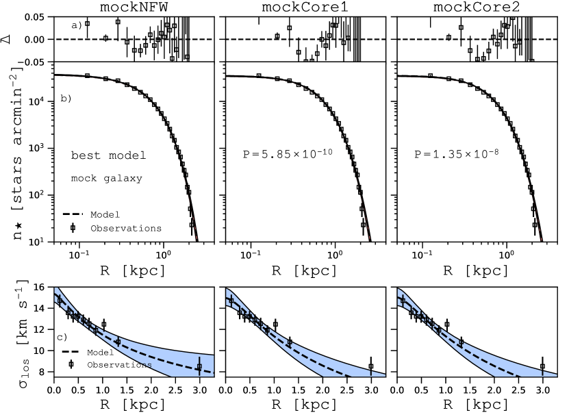
Figure 13: Columns, from left to right, refer to the best models of the mockNFW, mockCore1 and mockCore2 families, respectively. Top row of panels (a): residuals $\Delta\equiv(n_{\star}^{\text{obs}}-n_{\star})/n_{\star}$ between the model and the mock observed projected stellar density profile (points with error bars). Middle row of panels (b): projected number density profile of the model (dashed lines), compared with the mock observed profile (points with error bars). Bottom row of panels (c): line-of-sight velocity dispersion profile of the model (dashed lines), compared with the mock observed profile (points with error bars). In panels b and c the bands indicate the 1$\sigma$ uncertainties (see Section 3.2).

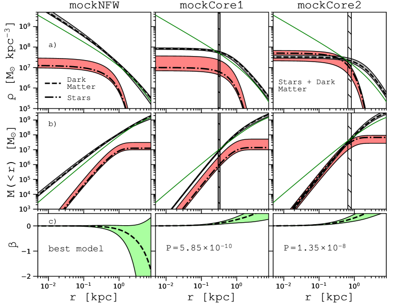
Figure 14: Columns, from left to right, refer to the best model of the mockNFW, mockCore1 and mockCore2 families, respectively. Top row of panels (a): stellar (dash-dotted line) and dark-matter (dashed line) density profiles. Middle row of panels (b): stellar (dash-dotted line) and dark-matter (dashed line) mass profiles. Bottom row of panels (c): anisotropy parameter profile (dashed line). The vertical black lines mark the halo core radius $r_{\rm c}$ for the cored families. In all panels the bands around the best fits indicate 1$\sigma$ uncertainty (see Section 3.2). The green curve in panels (a) and (b) show, respectively, the density and mass distributions of the mock dark-matter component (equation 52 and Table 7).

References

- Aaronson (1983) Aaronson M., 1983, ApJ, 266, L11
- Akaike (1998) Akaike H., 1998. Springer, New York, NY
- Amorisco & Evans (2011) Amorisco N. C., Evans N. W., 2011, MNRAS, 411, 2118
- Amorisco et al. (2013) Amorisco N. C., Agnello A., Evans N. W., 2013, MNRAS, 429, L89
- Arca-Sedda & Capuzzo-Dolcetta (2016) Arca-Sedda M., Capuzzo-Dolcetta R., 2016, MNRAS, 461, 4335
- Arca-Sedda & Capuzzo-Dolcetta (2017) Arca-Sedda M., Capuzzo-Dolcetta R., 2017, MNRAS, 464, 3060
- Battaglia et al. (2006) Battaglia G., et al., 2006, A&A, 459, 423
- Battaglia et al. (2008) Battaglia G., Helmi A., Tolstoy E., Irwin M., Hill V., Jablonka P., 2008, ApJ, 681, L13
- Battaglia et al. (2013) Battaglia G., Helmi A., Breddels M., 2013, New Astron. Rev., 57, 52
- Battaglia et al. (2015) Battaglia G., Sollima A., Nipoti C., 2015, MNRAS, 454, 2401
- Binney (2014) Binney J., 2014, MNRAS, 440, 787
- Binney & Piffl (2015) Binney J., Piffl T., 2015, MNRAS, 454, 3653
- Breddels & Helmi (2013) Breddels M. A., Helmi A., 2013, A&A, 558, A35
- Bullock & Boylan-Kolchin (2017) Bullock J. S., Boylan-Kolchin M., 2017, ARA&A, 55, 343
- Ciotti & Morganti (2010) Ciotti L., Morganti L., 2010, MNRAS, 408, 1070
- Cole & Binney (2017) Cole D. R., Binney J., 2017, MNRAS, 465, 798
- Cole et al. (2011) Cole D. R., Dehnen W., Wilkinson M. I., 2011, MNRAS, 416, 1118
- Das & Binney (2016) Das P., Binney J., 2016, MNRAS, 460, 1725
- Diakogiannis et al. (2017) Diakogiannis F. I., Lewis G. F., Ibata R. A., Guglielmo M., Kafle P. R., Wilkinson M. I., Power C., 2017, MNRAS, 470, 2034
- Einasto (1965) Einasto J., 1965, Trudy Astrofizicheskogo Instituta Alma-Ata, 5, 87
- El-Zant et al. (2001) El-Zant A., Shlosman I., Hoffman Y., 2001, ApJ, 560, 636
- Evans et al. (2016) Evans N. W., Sanders J. L., Geringer-Sameth A., 2016, Phys. Rev. D, 93, 103512
- Goerdt et al. (2006) Goerdt T., Moore B., Read J. I., Stadel J., Zemp M., 2006, MNRAS, 368, 1073
- Goerdt et al. (2010) Goerdt T., Moore B., Read J. I., Stadel J., 2010, ApJ, 725, 1707
- Hastings (1970) Hastings W. K., 1970, 57, 97
- Hui et al. (2017) Hui L., Ostriker J. P., Tremaine S., Witten E., 2017, Phys. Rev. D, 95, 043541
- Irwin & Hatzidimitriou (1995) Irwin M., Hatzidimitriou D., 1995, MNRAS, 277, 1354
- Jardel & Gebhardt (2012) Jardel J. R., Gebhardt K., 2012, ApJ, 746, 89
- Jeffreson et al. (2017) Jeffreson S. M. R., et al., 2017, MNRAS, 469, 4740
- King (1966) King I. R., 1966, AJ, 71, 64
- Kleyna et al. (2003) Kleyna J. T., Wilkinson M. I., Gilmore G., Evans N. W., 2003, ApJ, 588, L21
- Lima Neto et al. (1999) Lima Neto G. B., Gerbal D., Márquez I., 1999, MNRAS, 309, 481
- Mashchenko et al. (2006) Mashchenko S., Couchman H. M. P., Wadsley J., 2006, Nature, 442, 539
- Mateo (1998) Mateo M. L., 1998, ARA&A, 36, 435
- Metropolis et al. (1953) Metropolis A. W., Rosenbluth M. N., Teller A. H., Teller E., 1953, Journal of Chemical Physics, 21, 1087
- Michie (1963) Michie R. W., 1963, MNRAS, 126, 499
- Minor et al. (2010) Minor Q. E., Martinez G., Bullock J., Kaplinghat M., Trainor R., 2010, ApJ, 721, 1142
- Mo & Mao (2004) Mo H. J., Mao S., 2004, MNRAS, 353, 829
- Muñoz-Cuartas et al. (2011) Muñoz-Cuartas J. C., Macciò A. V., Gottlöber S., Dutton A. A., 2011, MNRAS, 411, 584
- Navarro et al. (1996a) Navarro J. F., Eke V. R., Frenk C. S., 1996a, MNRAS, 283, L72
- Navarro et al. (1996b) Navarro J. F., Frenk C. S., White S. D. M., 1996b, ApJ, 462, 563
- Nipoti & Binney (2015) Nipoti C., Binney J., 2015, MNRAS, 446, 1820
- Peñarrubia et al. (2008) Peñarrubia J., McConnachie A. W., Navarro J. F., 2008, ApJ, 672, 904
- Piffl et al. (2015) Piffl T., Penoyre Z., Binney J., 2015, MNRAS, 451, 639
- Pontzen & Governato (2012) Pontzen A., Governato F., 2012, MNRAS, 421, 3464
- Posti et al. (2015) Posti L., Binney J., Nipoti C., Ciotti L., 2015, MNRAS, 447, 3060
- Pryor & Meylan (1993) Pryor C., Meylan G., 1993, in Djorgovski S. G., Meylan G., eds, Astronomical Society of the Pacific Conference Series Vol. 50, Structure and Dynamics of Globular Clusters. p. 357
- Read & Gilmore (2005) Read J. I., Gilmore G., 2005, MNRAS, 356, 107
- Read et al. (2017) Read J. I., Iorio G., Agertz O., Fraternali F., 2017, MNRAS, 467, 2019
- Richardson & Fairbairn (2014) Richardson T., Fairbairn M., 2014, MNRAS, 441, 1584
- Salucci et al. (2012) Salucci P., Wilkinson M. I., Walker M. G., Gilmore G. F., Grebel E. K., Koch A., Frigerio Martins C., Wyse R. F. G., 2012, MNRAS, 420, 2034
- Sánchez-Salcedo et al. (2006) Sánchez-Salcedo F. J., Reyes-Iturbide J., Hernandez X., 2006, MNRAS, 370, 1829
- Sanders & Binney (2016) Sanders J. L., Binney J., 2016, MNRAS, 457, 2107
- Sanders & Evans (2015) Sanders J. L., Evans N. W., 2015, MNRAS, 454, 299
- Schwarzschild (1979) Schwarzschild M., 1979, ApJ, 232, 236
- Sersic (1968) Sersic J. L., 1968, Atlas de galaxias australes
- Shapley (1938) Shapley H., 1938, Nature, 142, 715
- Strigari et al. (2008) Strigari L. E., Bullock J. S., Kaplinghat M., Simon J. D., Geha M., Willman B., Walker M. G., 2008, Nature, 454, 1096
- Strigari et al. (2017) Strigari L. E., Frenk C. S., White S. D. M., 2017, ApJ, 838, 123
- Tollet et al. (2016) Tollet E., et al., 2016, MNRAS, 456, 3542
- Vasiliev (2018) Vasiliev E., 2018, preprint, (arXiv:1802.08239)
- Walker & Peñarrubia (2011) Walker M. G., Peñarrubia J., 2011, ApJ, 742, 20
- Walker et al. (2009) Walker M. G., Mateo M., Olszewski E. W., 2009, AJ, 137, 3100
- Watkins et al. (2013) Watkins L. L., van de Ven G., den Brok M., van den Bosch R. C. E., 2013, MNRAS, 436, 2598
- Williams & Evans (2015) Williams A. A., Evans N. W., 2015, MNRAS, 448, 1360
- Wolf et al. (2010) Wolf J., Martinez G. D., Bullock J. S., Kaplinghat M., Geha M., Muñoz R. R., Simon J. D., Avedo F. F., 2010, MNRAS, 406, 1220
- Zhu et al. (2016) Zhu L., van de Ven G., Watkins L. L., Posti L., 2016, MNRAS, 463, 1117
- de Blok (2010) de Blok W. J. G., 2010, Advances in Astronomy, 2010, 789293
- de Boer et al. (2012) de Boer T. J. L., et al., 2012, A&A, 544, A73