Signatures of Cosmic Reionization on the 21cm 2- and 3-point Correlation Function I: Quadratic Bias Modeling
Abstract
The three-point correlation function (3PCF) of the 21cm brightness temperature from the Epoch of Reionization (EoR) probes complementary information to the commonly studied two-point correlation function (2PCF) about the morphology of ionized regions. We investigate the 21cm 2PCF and 3PCF in configuration space using semi-numerical simulations and test whether they can be described by the local quadratic bias model. We find that fits of bias model predictions for the 2PCF and 3PCF deviate from our measurements by at scales above the typical size of ionized regions ( Mpc) and at early times with global neutral fractions of . At later times and smaller scales these deviations increase strongly, indicating a break down of the bias model. The 2PCF and 3PCF fits of the linear bias parameter agree at the level for different EoR model configurations. This agreement holds, when adding redshift space distortions to the simulations. The relation between spatial fluctuations in the matter density and the 21cm signal, as predicted by the bias model, is consistent with direct measurements of this relation in simulations for large smoothing scales ( Mpc). From this latter test we conclude that negative amplitudes of the 21cm 3PCF result from negative bias parameters, which describe the anti-correlation between the matter over-densities and the 21cm signal during the EoR. However, a more detailed interpretation of the bias parameters may require a description of non-local contributions to the bias model.
keywords:
cosmology: Reionization - methods: statistical - numerical - analytical1 Introduction
Observations with upcoming radio telescopes, such as the low frequency segment of the Square Kilometre Array (SKA-Low)111www.skatelescope.org and the Hydrogen Epoch of Reionization Array (HERA)222www.reionization.org, will ring in a new era of cosmology, allowing us to observe the distribution of neutral hydrogen (HI) in the early universe at unprecedented scales. These observations will provide novel insights into how the first luminous objects ionized their surrounding gas. This so-called Epoch of Reionization (EoR) leads to the almost completely ionized universe that we see today and can be characterized by the large-scale HI distribution at different times. This distribution is traced by the light emitted at the wavelength of 21 centimeter due to the HI hyperfine transition. Today we can observe this light as radio signals, since it was redshifted during its journey through the expanding universe (Field, 1958). The 21cm signal is expected to show large-scale spatial fluctuations, which reflect the inhomogeneous matter distribution in the universe. Current EoR models suggest that these fluctuations are overlaid by patches without any 21cm emission, which are filled with ionized gas around the first luminous objects (e.g. Sokasian et al., 2004). The upcoming 21cm observations contain therefore not only information about how matter density fluctuations grow with time due to gravity, but also about how the first luminous objects form and transfer energy to the intergalactic medium (e.g. Furlanetto et al., 2006; Pritchard & Loeb, 2012). Extracting this information from observations requires a statistical description of the 21cm fluctuations. Correlation functions have proved to be useful tools for this purpose. Studies on the two-point correlation function of the 21cm EoR signal, or the power spectrum as its Fourier space counterpart, revealed its high sensitivity to the underlying EoR model (e.g. Pober et al., 2014). This opens up the possibility to use this statistics for constraining EoR models with future observations (e.g. Liu & Parsons, 2016). However, a restriction to one or two-point statistics prevents access to information on the morphology of the ionized regions, which is one of the most prominent features in simulated maps of the 21cm signal. Only recently studies probe this additional information using the three-point correlation in Fourier space, i.e. the bispectrum (e.g. Shimabukuro et al., 2016). The results revealed a strong dependence of the bispectrum on the scale, as well as on the shape of the triangles from which this statistics is measured (Majumdar et al., 2018). This additional information from the bispectrum can strongly improve the constraints on EoR model parameters from power spectrum measurements (Shimabukuro et al., 2017).
Deriving such constraints from observations requires predictions for the 21cm statistics, which can be obtained from either theoretical modeling, or from simulations. In the latter case a large number of simulations is needed for a sufficiently dense sampling of the high dimensional EoR parameter space. In addition, these simulations need to cover a wide dynamical range to accurately predict the formation of ionizing sources at scales of Mpc and simultaneously the transfer of their radiation to the intergalactic medium on scales of up to Mpc. Furthermore, the simulation volume needs to be sufficiently large ( Mpc) to allow for precise measurements of the chosen statistics. These requirements can be met currently only with approximate simulation methods or emulation techniques (e.g. Mesinger et al., 2011; Schmit & Pritchard, 2018).
Alternatively to simulations, predictions for the 21cm correlation functions can be obtained from theoretical models. Such models have been presented for the 21cm power spectrum by Furlanetto et al. (2004); Lidz et al. (2007). To our knowledge, however, the only model for the 21cm bispectrum is restricted to the simplistic case of randomly distributed ionized spheres, which shows similarities with simulation results only at small scales (Bharadwaj & Pandey, 2005; Majumdar et al., 2018).
The goal of this work is to further develop the theoretical understanding of the two-point and, in particular, the three-point correlation functions (hereafter referred to as “2PCF” and “3PCF”, respectively) of the 21cm brightness temperature, based on measurements in simulations. Our investigation of the 21cm 3PCF is performed for the first time in configuration space, which may simplify the physical interpretation of our results. To interpret our measurements, we employ the quadratic bias model, which has been developed to model the 3PCF of large-scale halo and galaxy distributions (Fry & Gaztanaga, 1993). In the context of 21cm statistics, this model assumes that the matter density in a given volume of the universe determines the 21cm brightness temperature in that same volume, while the form of this deterministic relation is characterized by a set of free parameters. This bias model allows for a perturbative approximation of the 21cm 2PCF and 3PCF, which depend at leading order on the two free bias parameters and .
We test the bias modeling using a set of realizations of reionization simulations, which were performed with the semi-numerical code 21cmFAST (Mesinger et al., 2011). These simulations differ only in their initial conditions of random density fields, and cover a total volume of , providing robust measurements of the 21cm 2PCF and 3PCF, as well as estimates for their error covariance.
This paper is organized as follows. We start by presenting our simulation in Section 2. The bias model is introduced in Section 3 in which we also verify how well its prediction for the 2PCF and the 3PCF agree with the measurements in the simulations. As the second step in the model validation, we compare the 2PCF and 3PCF fits of bias parameters in Section 4. Using these bias parameters, we further test in that section how well the relation between the matter and 21 brightness temperature, as predicted by the bias model, holds using direct measurements in simulations. We summarize our results and draw conclusions from our analysis in Section 5.
2 Simulation
Our analysis is based on simulations of three-dimensional maps of the matter density and the 21cm brightness temperature, using the semi-numerical code 21cmFAST (Mesinger et al., 2011). For a fast production of 21cm maps, 21cmFAST first derives the evolved matter density distribution using the Zel’dovich approximation, starting from an initial Gaussian random field. The three-point statistics of such distributions have been shown to deviate significantly from those derived with full N-body simulations at low redshifts (Scoccimarro, 1997; Leclercq et al., 2013). In order to investigate how strongly our results are affected by the Zel’dovich approximation we generate additional matter density distributions using the code L-PICOLA. This code employs the COLA method to approximate N-body simulations. This type of simulations reproduces two- and three-point statistics of matter distributions from full N-body simulations with percent level accuracy, while being computationally less expensive (Tassev et al., 2013; Howlett et al., 2015).
The mean matter and baryon densities are set to and , respectively, with the Hubble parameter . The scalar spectral index of primordial density fluctuations is set to and the initial power spectrum at is obtained from the Eisenstein & Hu (1998) transfer function. These parameters are identical for the L-PICOLA runs, besides the initial redshift, which was set to . These latter simulations where run down to in time steps. The ionized regions and the resulting 21cm signals are computed from the matter field in a second step with a semi-numerical approach, which is based on the excursion set formalism (Furlanetto et al., 2004). It uses the argument that a given region (i.e. simulation cell) is ionized when the fraction of collapsed matter fluctuations with a mass above , which reside within a sphere with radius around the regions center, passes a certain threshold, i.e.

| (1) |
where is the ionization efficiency parameter and can be interpreted as mean free path length for photons in the intergalactic medium. The neutral fraction characterizes the ionization state of that region and corresponds to its local fraction of HI with respect to its total number of hydrogen atoms. The collapsed fraction is given by
| (2) |
The normalized spatial fluctuation of the total matter density, , around the universal mean is defined as
| (3) |
Note that the fluctuations , with which we will work later as well, are defined analogously. We set the critical amplitude of matter fluctuations for spherical collapse to , is the large-scale matter fluctuation around the potentially ionized region, smoothed with a Fourier space top-hat filter on the scale and is the variance of the matter density field for a top-hat filter in configuration space with radius . The inconsistent filtering for and allows for faster computations of around each simulation cell, since the Fourier space filtering is done by a simple cut of the power spectrum. A -space top-hat filter is in principle also convenient for theory applications, since for a Gaussian random field, the differences between at different smoothing radii (i.e. the steps of the excursion set trajectories) are uncorrelated. However, a detailed physical interpretation of the simulation parameters would require a consistent filtering for and in configuration space, since that is where the physical processes, which drive the ionization (e.g. the radiation transport) are most conveniently described. For the top-hat filter encloses on average the minimum mass for ionizing fluctuations . The minimum mass is derived from the minimum temperature for ionization via
| (4) |
(e.g. Barkana & Loeb, 2001), where is the non-linear matter fluctuation at virialization, which was approximated by Bryan & Norman (1998) as with . The mean molecular weight is set in our simulations to for ionized hydrogen and singly-ionized helium. Once the neutral fraction has been computed for each simulation cell, the 21cm brightness temperature is obtained via
| (5) |
with
(e.g. Furlanetto, 2006) for an optically thin inter galactic medium. The term is proportional to the local HI density, assuming a linear relation between the hydrogen and the full matter densities. Mesinger et al. (2011) found that this assumption breaks down at scales below Mpc, but holds at larger scales which we study in this work.
We focus on the regime in which the gas has been significantly heated, so that the spin temperature is much greater than the Cosmic Microwave Background (CMB) temperature . This approximation is reasonable after the onset of cosmic reionization when the fluctuations of the 21cm signal are dominated by those of the neutral fraction induced by the inhomogeneous reionization (e.g. Zaldarriaga et al., 2004; Pritchard & Furlanetto, 2007; Mesinger et al., 2011), but may need to be revisited for a more detailed analysis.
We compute the correlations of the 21cm signal with and without corrections due to redshift space distortions (hereafter referred to as RSD). Neglecting RSD may be appropriate for analysis of projected 21cm signals in redshift bins. However, studies on three dimensional 21cm power spectra found notable contributions on large scales, in particular for early times with high neutral fraction (McQuinn et al., 2006; Mesinger & Furlanetto, 2007), in which case a detailed modelling of 21cm redshift space distortion should be taken into account. For selected cases we therefore study the effect of RSD on the 21cm 2PCF and 3PCF, comparing a simplified RSD prescription implemented in 21cmFAST with a more realistic model MMRRM. The MMRRM code (Mao et al., 2012) is based on the sophisticated investigation of the effects of peculiar velocity on the observed 21cm signal, which manifests in two aspects: the 21cm brightness temperature is modified, and a distance separation along line-of-sight is resized in redshift space, both according to the velocity gradient. The net effect on the 21cm brightness temperature in redshift-space is , where is the neutral hydrogen density fluctuations in redshift space. We refer readers to Mao et al. (2012) for a detailed discussion of this methodology. On the other hand, the 21cmFAST code has an option to implement a simplistic prescription for 21cm RSD, in which a maximum for the absolute value of the velocity gradient, , is enforced by hand to avoid artificial singularity.
We employ three reionization models which are characterized by different sets of parameters as summarized in Table 1.
| model | [K] | |
|---|---|---|
| A | ||
| B | ||
| C |
The maximum filtering scale is set to Mpc for all three models. Model A serves as our fiducial model throughout the analysis unless the use of model B and C is specified explicitly.
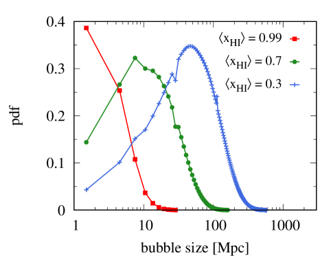
All simulations are run in cubical volumes of ( with periodic boundary conditions on Cartesian grids with () cells and with the side lengths of cells of () Mpc, for the matter (HI) fields, respectively. RSDs are applied along one simulation axis in a plane-parallel approximation. To estimate the error covariance of our measured statistics, we generate a set of independent realizations with different random initial conditions for the fiducial model A, which cover a total volume of . For model B and C we use realizations to reduce computational costs. For the L-PICOLA runs we restrict our analysis to just realizations with particles due to the relatively high computational costs compared to simulation based on the Zel’dovich approximation. In Fig. 1 we show the simulated distributions of the matter density fluctuations in one realization and the corresponding 21cm brightness temperature distributions from model A without RSDs at different redshifts. One can see how ionized regions start to form around the largest matter overdensities at high redshifts and connect with each other, as they grow with decreasing redshift. This growth progresses relatively fast compared to the growth of the large-scale matter density fluctuations. The redshift evolution of the global volume-weighted neutral fraction is shown in Fig. 2 for all three reionization models. This figure illustrates on one hand how reducing the minimum virial temperature of halos that host ionizing sources in model B from the fiducial value in model A accelerates the global ionization process, as ionizing sources can now reside in lower mass halos (see equation (4)), which increases their total number density. Reducing the reionization efficiency in model C on the other hand delays the reionization process, as a larger collapsed fraction is needed for ionizing a given region (see equation (1)). In Fig. 3, we show the probability distribution function (pdf) of the sizes of ionized regions (or HII bubbles), averaged over different random realizations. The sizes are measured by 21cmFAST by choosing random positions in ionized regions and measuring the distance from each of these positions to the neutral phase in a randomly chosen direction. The distribution of these distances is interpreted as the bubble size pdf. These pdfs cover scales between and Mpc, while their maxima lie at around , and Mpc for , and , respectively.

3 Biased correlation functions
We quantify the clustering of the matter density and 21cm brightness temperature with the 2PCF and 3PCF. The convenience of these statistics arises from the fact that they are well defined and have been extensively investigated in galaxy clustering analysis (e.g. Bernardeau et al., 2002). The studies therein implied that the correlation functions of some tracers of the total matter density field can be related to those of the latter via the so-called bias model, as detailed below.
3.1 Quadratic bias model
In the context of 21cm observations, the local bias model corresponds to a function , which describes a deterministic relation between the fluctuations in the matter density and those in the 21cm brightness temperature , defined by equation (3), in a region of size around a given position , i.e. . The term “local” refers to the assumption that is solely determined by in the same region. This assumption can be violated, for instance, by ionizing radiation originating from overdensities outside of the region (e.g. Furlanetto et al., 2004), or the tidal field induced by the surrounding matter distribution, which affects the formation of halos that host the ionizing sources in that region (Chan et al., 2012; Baldauf et al., 2012). However, for sufficiently large scales and early stages of reionization, the deterministic approximation might be adequate, as we will see later in this analysis.
The form of the bias function is unknown at this point, but we can approximate it with a Taylor series around , assuming that varies only weakly with , i.e , where are the bias parameters. The bias model provides a tool to relate the 2PCF and 3PCF of to the corresponding statistics of the underlying matter field. For establishing these relations for third-order statistics at leading order in , we need to expand the bias function at least to second order (Fry & Gaztanaga, 1993), i.e.
| (6) |
Requiring sets the constrain , where is the variance of the matter density fluctuations. Here denotes the spatial average of the universe. The remaining free parameters and are referred to as linear and quadratic bias parameters, respectively.
3.2 Two-point correlation functions (2PCF)
The 2PCF can be defined via the product of fluctuations at two different positions
| (7) |
where are the fluctuations of some observable at the position , i.e. , and denotes the average over all possible orientations and translations of the pairs, separated by the distance . We denote the 2PCFs of the matter density fluctuations and 21cm brightness temperature fluctuations (referred to as “21cm 2PCF”) as and , respectively. Due to the average over all orientations, the 2PCF is only sensitive to the scale dependence of the clustering, but not to the shape of large-scale structures. As a second-order statistic, it is also insensitive to a skewness in the one-point probability distribution of the fluctuations . This additional information can be accessed via the 3PCF, which will be introduced in Section 3.3. Our 2PCF measurements are performed on a grid of cubical cells with Mpc side lengths. We thereby measure the fluctuations and in each cell and then search for pairs of cells to obtain the average from equation (7).

We start our analysis by comparing the mean 21cm 2PCF over all realizations from our three EoR models without RSD at two fixed redshifts in the top panel of Fig. 4. We find a significant dependence of the 2PCF on the EoR model at a given redshift as well as a strong redshift evolution for a given EoR model. Results based on the matter fields from the Zel’dovich approximation and the L-PICOLA runs (displayed for model A as dots and crosses repsectively) show no significant deviations.
Differences between measurements for different EOR models and redshifts can be approximated by a single scale independent shift of the amplitude. This behaviour illustrates the limited constraining power of the 21cm 2PCF on EoR models, which depend on several free parameters. When comparing results at fixed volume weighted global neutral fractions (bottom panel of Fig. 4), we find only a percent level dependence of the 21cm 2PCF on the EoR model (note that the global neutral fractions are only fixed at percent level accuracy). This finding can be understood with the following consideration. The condition for the ionization of a given region from eq. (1) can be rewritten with eq. (2) in terms of an ionization barrier, i.e. , with , where , is the variance of the matter field at and is the linear growth factor (e.g. Furlanetto et al., 2004). The terms in this expression that depend on and are degenerate with the redshift dependent growth factor. A certain spatial distribution of neutral fractions can hence be obtained by different combinations of the redshift and the EoR model parameters. This argument implies that also (eq. (5)) is roughly model independent at a fixed global neutral fraction, given that the evolution of is very weak at the high redshifts considered in this work in comparison with the strong evolution of (see Fig. 1). However, this result is specific to the excursion set based simulations, and might break down to some degree in more complex EoR models.
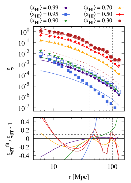
To study the relation between the matter and 21cm 2PCF, we show both correlations together in Fig. 5. The matter 2PCF, displayed at only two redshifts for clarity, shows the expected scale dependence, while the amplitude increases weakly with decreasing redshifts (decreasing neutral fractions), due to the slow growth of matter fluctuations at early times. We have verified that these measurements agree with theory predictions based on the initial power spectrum of the simulation for Mpc. Tests with simulations in boxes with twice the side length (i.e. Mpc) revealed that our mean 2PCF measurements at scales above Mpc are significantly affected by the limited box size, since the latter causes an artificial cut-off at large wavelength modes (see Appendix A). We therefore exclude 2PCF measurements for scales above Mpc from our analysis.
The 21cm 2PCF, displayed for model A without RSD as solid symbols at various redshifts in Fig. 5, shows a much stronger redshift evolution than the matter 2PCF. We find that the amplitude first decreases, between and , before it increases strongly for lower redshifts with lower neutral fractions. At large scales ( Mpc) the shapes of the 21cm 2PCFs are very similar to those of the matter 2PCF, while being shifted by a roughly constant factor. This latter behaviour can be expected from the bias model, since equation (6) delivers at leading order in
| (8) |
Interestingly, the 21cm 2PCF at does not follow this trend, as its amplitude falls more steeply with scale, indicating a very week clustering of the 21cm signal. This effect will be be discussed in Section 4.1. Note that alternatively to equation (8), the relation between the and can be derived by expanding the former in terms of some 2nd, 3rd, and 4th order statistics between neutral fraction and/or density fields and modelling them with physically motivated approximations. However, those approximations can limit their accuracy (e.g. Furlanetto et al., 2004; Lidz et al., 2007; Raste & Sethi, 2018). Furthermore, this approach becomes more challenging for statistics beyond the second order such as the 3PCF.
We fit the linear bias model for from equation (8) to our measurements between Mpc via a minimization, as detailed in Appendix C. Note that we can thereby only infer the absolute value of the linear bias parameters, since it appears as in equation (8). However, we will see later on that can take positive as well as negative values. The fits to equation (8) are shown as solid lines in the top panel of Fig. 5. They deviate from the measurements by () within the fitting range for (), as shown in the bottom panel of Fig. 5. The strong deviations for lower global neutral fractions, as well as for indicate a breakdown of the local bias model at these stages of reionization. Deviations from the fits increase as well at small scales below Mpc, which correspond roughly to the typical sizes of ionized regions, as shown in Fig. 3. Deviations at large scales above Mpc may partly result from the aforementioned box size effect.
Note that the 21cm 2PCFs which we use for the fits do not include RSDs, which will not be the case in future observational data sets. In order to obtain a rough insight into how RSDs would affect the 21cm 2PCF, we show results from simulations with RSDs from the MMRRM model as open symbols in Fig. 5. The results show that the RSDs cause a strong increase of the 21cm 2PCF at large scales and early time ( ), while the latter takes a similar shape as the matter 2PCF. At later times ( ) the effect of RSDs decreases strongly. A more detailed picture can be obtained from Fig. 6, which shows the relative deviations between the 21cm 2PCF for model A with and without RSDs. We compare results from the MMRRM model to those from a simplified RSD model, implemented in 21cmFAST.
The MMRRM model predicts a strong increase of the 21cm 2PCF by up to a factor of at large scales for and a strong decrease of up to at due to RSD. At later times ( ), the decrease is strongest at small scales ( Mpc) with shift of the amplitude and becomes insignificant at Mpc. The simplified RSD model from 21cmFAST tends to underpredict the RSD effect on the 2PCF, in particular at late times. However, at early times, where RSD effects are most significant, the approximate implementation works reasonably well. We conclude that RSDs need to be taken properly into account, when interpreting future observational data sets, but we focus in this work on simulations without RSD to develop a physical understanding of how the matter and 21cm correlations are related to each other.

3.3 3-point correlation functions (3PCF)
The 3PCF is defined analogously to the 2PCF as
| (9) |
The positions of the fluctuations form a triangle, with three legs of the sizes , , and . Similar to the 2PCF, denotes the average over all possible triangle orientations and translations. We denote the 3PCFs of the matter and 21cm brightness temperature fluctuations (referred to as “21cm 3PCF”) as and , respectively. Our 3PCF measurements are performed on the same type of grid on which we compute the 2PCF. To search for triplets of grid cells, we employ the algorithm described by Barriga & Gaztañaga (2002). This algorithm delivers measurements for triangles with two fixed legs () and varying leg sizes . The cell size is set to or Mpc for small and large triangles, respectively, to optimize the computation time. We have verified for the triangle configurations and Mpc, that the effect of the cell size (or smoothing scale) on the 3PCF measurements is within the errors, except for triangles for which is comparable to the cell size (see also Hoffmann et al., 2018). In general, the 3PCF depends on the smoothing scale, even at large scales, while we expect this smoothing effect on our bias measurements described below to be small, based the aforementioned test.
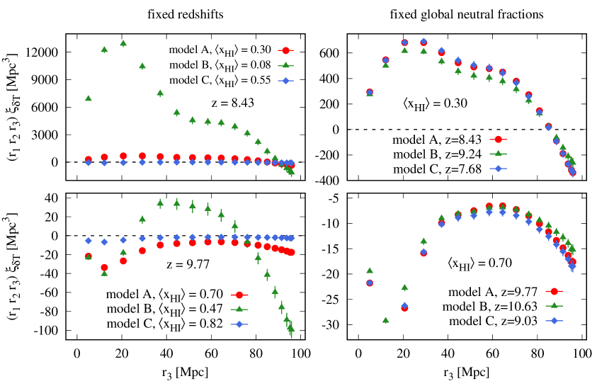
We show measurements of the 21cm 3PCF for the three EoR models, summarized in Table 1, without RSDs at the redshifts and in the left panels of Fig. 7. The measurements are done using triangles with Mpc and are displayed versus the third triangle leg , for corresponding opening angles (the angle between and ) between and degrees. These measurements reveal a high sensitivity of the 21cm 3PCF to variations of the EoR model parameters. The strong change of the 3PCF amplitude as well as its shape stand in contrast to our 2PCF measurements, for which we found changes due to variations of EoR parameters to be well described by a simple shift of the amplitude (Fig. 4). This finding illustrates that 3PCF contains additional information with respect to the 2PCF, which may be used to tighten constraints on EoR models with future observations. In the right panel of Fig. 7 we compare the 21cm 3PCF from different models at fixed global neutral fractions. We find a relatively weak () dependence of the measurements on the model parameters in that case, compared to the change with redshift. This result lines up with our finding for the 2PCF from the Fig. 4 and may be explained with the same argument outlined in Section 3.2.

We continue our study by investigating the relation between the 3PCF of the 21cm and the matter field in Fig. 8 for two triangle configurations with fixed legs and Mpc versus at redshift ( ). The matter 3PCF, displayed in the top panels, has positive values for collapsed and relaxed triangles (small and large respectively), while being negative for half open triangles. This typical shape is a signature of the filamentary structure of the cosmic web (e.g. Bernardeau et al., 2002), and hence provides additional information about the dark matter distribution to which one- or two-point statistics are not sensitive.
These results are compared to the matter 3PCF from the L-PICOLA runs, which are shown as grey open circles in the same figure. The shape of the matter 3PCF from both types of simulations are slightly different from each other. However, these differences are small compared to the overall change of the 3PCF with triangle configuration and lie within the uncertainties for triangles with Mpc. The corresponding measurements for the 21cm 3PCF from model A without RSD are shown in the bottom panels of Fig. 8. We compare also these measurements to results based on the L-PICOLA runs and find again only small deviations compared to the dependence of the amplitude on triangle configuration and EoR model.
Interestingly these 21cm 3PCF measurements are negative for all triangles, while their overall shape appears to be similar to the matter 3PCF. This indicates that there is a physical relation between both statistics. In analogy to the 2PCF, this relation can be approximated by a perturbative expansion of the 21cm 3PCF, using the bias model. From equation (6), one finds, at leading order
| (10) |
(Fry & Gaztanaga, 1993). The hierarchical three-point correlation, , with , is shown as dashed-dotted lines in the top panels of Fig. 8.
We derive and from the 3PCF by fitting equation (10) to our measurements. The fits, shown as red line in the bottom panels of Fig. 8, are obtained from a minimization. The values are computed via a Singular Value Decomposition (SVD) of the covariance matrix (shown in Fig. 22), as suggested by Gaztañaga & Scoccimarro (2005) to reduce the impact of noise in the covariance on our fits (see Appendix C for details). We fit the model only to measurements from triangles, for which all legs are in the range Mpc. This selection is motivated by our 2PCF results, which showed that the bias model prediction breaks down at smaller scales, while measurements at large scales may be affected by the limited box size (see Section 3.2).
Our fits are in reasonable agreement with the measurements within the fitting range, which shows that the quadratic bias model can describe the dominating part of the 21cm 3PCF signal at large scales. However, the fits deviate strongly from our measurements at small scales, below the minimum fitting scale. This indicates a break down of the bias model, according to which a given set of fitted bias parameters should describe the 21cm 3PCF at all scales.
The redshift evolution of the 21cm 3PCF is shown for triangles with Mpc versus in Fig. 9. We use again model A, while we now show measurements for simulations without RSD as well as with RSD from the MMRRM model. Focusing first on results without RSD, we find that on large scales and at early times ( Mpc, ) the 21cm 3PCF has a negative amplitude and a positive slope for this triangle configuration. At later times the large-scale amplitude becomes positive, while the slope becomes negative at large scales. Again, this behaviour is well described by the fits to equation (10) on scales above Mpc, while we find strong deviations between fits and measurements at smaller scales. An interesting feature at small scales is the local minimum of the 3PCF without RSD at and Mpc for and , respectively. This feature may be associated with the a small scale increase of the 21cm bispectrum, predicted by Majumdar et al. (2018) for randomly distributed ionized bubbles. These authors also found a similar feature in the 21cm bispectrum measurements from simulations. However, more detailed studies are needed for understanding this effect.
As in Fig. 8 we compare in Fig. 9 our main results for the 21cm 3PCF based on the Zel’dovich approximation to those from the L-PICOLA runs, which are shown as grey open circles at the highest and lowest redshifts with and respectively. We find again that the differences between results from both types of simulations are small, in particular at large scales, compared to the change of the amplitude with triangle configurations and redshift. We therefore do not expect the conclusions of this investigation to be significantly affected by the usage of the Zel’dovich aproximation.
The 21cm 3PCFs from simulations with RSD appear to be very similar to those from simulations without RSD at large scales and late times ( Mpc, ), while at smaller scales as well as at earlier times results from both cases deviate more significantly. The RSD results can also be well fitted with the quadratic bias at large scales. However, the RSD change the physical meaning of the fitted bias parameters, since in that case the 21cm 3PCF does not only depend on the relation between the matter field and the hydrogen distributions, but also on the hydrogen velocity.

In Fig. 10 we compare the relative deviations between the 21cm 3PCF from simulations with model A with and without RSD for two triangle configurations with fixed legs of and Mpc at different sizes and different global neutral fractions. We find the RSD effect to depend strongly on the specific triangle scale and configurations, as well as on redshift. For the MMRRM model the changes in the amplitude vary between (e.g. for Mpc at ) and a factor of (for the largest values at ). The relative changes of the 21cm 3PCF due to RSD are overall stronger, than those which we found for the 21cm 2PCF in Fig. 6. However, note that even strong changes in the 3PCF amplitude can lead to relatively small changes in the bias parameters (see Section 4), since enters equation (10) with up to the power of three. The absolute change of the 3PCF amplitude from simulations with the simplified RSD model, implemented in 21cmFAST is lower than predicted by the more physical MMRRM model, which lines up with our 2PCF results from Fig. 6.

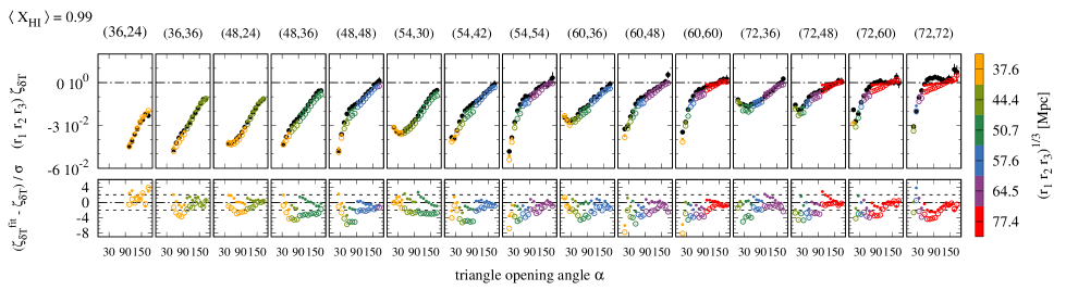
We now aim at testing the quadratic bias model prediction for the 21cm 3PCF from model A without RSD on a wider range of scales by jointly fitting larger sets of triangles. In Fig. 11 we show 3PCF measurements from triangle configurations, defined by the fixed legs at the redshifts and , with and respectively. The 3PCF is multiplied by to decrease the strong scale dependence of the signal, simplifying a visual comparison of the different measurements. Note that this multiplication modifies the overall shape of the 3PCF, which can be seen by comparing results for Mpc to the results from Fig. 9. In order to verify the scale dependence of the 3PCF bias model fitting performance and the resulting bias parameters, we fit the measurements in triangle scale bins, as marked by colour in Fig. 11. The triangle scale is thereby defined as , while each scale bin contains triangles. We find deviations between fits and measurements of roughly for the largest triangle scale bin with Mpc at both redshifts. For the smallest scale bin with Mpc, deviations tend to be more significant, with up to () for (). These values can correspond to relative deviations of more than for , while we find deviations for Mpc and higher global neutral fractions (see Fig. 20). The latter figure also suggests that the lower significance of deviations at large scales might be attributed to an increase of the measurement errors with scale. However, one could also expect that the perturbative approximations incorporated in the bias model should work better at larger scales, where non-linearities are smaller. To verify the impact of the covariance estimate on the fits, we neglect off-diagonal elements in the covariance for computing the deviations in eq. (14). The resulting fits, shown as colored dots in Fig. 11, indicate that that these off-diagonal covariance matrix elements can have a strong impact on the fits and should not be ignored. It is therefore important to reduce noise in the covariance estimates, which we attempt by using the aforementioned SVD technique and a relatively large number of realizations.
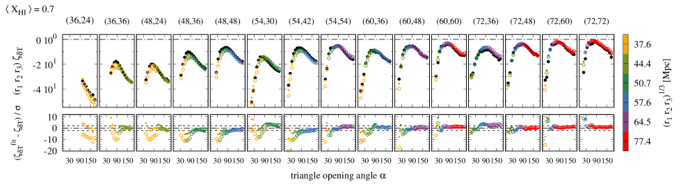
The goodness of these fits is shown as the minimum per degree of freedom () in Fig. 12 versus the mean triangle scale per bin for model A without RSD at various volume weighted neutral global fractions. The degree of freedom is here the number of modes in the covariance matrix with singular values above the shot-noise limit, from which we compute the values (see Fig. 23). In addition to the values based on fits in scale bins with triangles, we also show results for smaller and larger bins with and triangles, respectively, verifying the robustness of our results. We find that for scales above Mpc, the values range between and , independently from the binning. Given our small measurement errors, which result from the large total simulation volume of the realizations, the goodness of fit values indicate a reasonable agreement between model and measurements for . The values strongly increase for lower global eutral fractions, which is another indication for the break down of the leading order 3PCF bias model. The increase of the values at small scales might be attributed to the same effect. However, the smaller measurement errors at small scales also increase the significance of deviations between measurements and model fits, as we already concluded from Fig. 11.
4 Bias comparison
In the previous section, we found that the leading order bias expansions of the 21cm 2PCF and 3PCF provide reasonable fits to the measurements in our simulations, in particular at early times of reionization and at large scales. In this section, we will focus on this regime, studying the bias parameters obtained from these fits in two ways. We start by verifying the consistency of the bias parameters, obtained from the 2PCF and the 3PCF fits in Section 4.1. In Section 4.2 we will test if the deterministic quadratic bias model is in agreement with the relation between the fluctuations of and matter, which we can measure directly in the simulations.
4.1 Bias from correlation functions
Examples of our 3PCF bias constraints are shown in Fig. 13 for our fiducial model A without RSD at different volume weighted global neutral fractions as and confidence regions in the parameter space. These results are obtained from triangles with an average scale of Mpc, shown as the largest scale bin in Fig. 11. We find the linear bias to be positive for and negative at later times, with values between . The initially positive values of our measurements originate from the fact that the HI distribution follows the matter density before reionization starts. Later on, the first ionized regions with zero 21cm emission form around the largest matter overdensity regions (see Fig. 1), leading to an anti-correlation between the 21cm signal and the matter fluctuations, as described by a negative bias (see Section 4.2 for a more detailed discussion). The change of from positive to negative values with time is consistent with the decrease of the 2PCF amplitude at early times and its increase at later times (Fig. 5), since the latter depends on . The transition around manifests itself in the low 2PCF amplitude at , shown in the same figure. The quadratic bias is negative for and positive at later times with lower global neutral fractions. It reaches larger absolute amplitudes than , in the rage with a minimum of at . The degeneracy between the two parameters is relatively weak, while the uncertainty on is significantly larger than for . The latter result might be attributed to the fact that is more sensitive to changes in than in since these parameters appear in equation (10) at up to third and linear order respectively.

To verify the scale dependence of our 3PCF bias measurements, we display and in Fig. 14 for model A without RSD, derived from triangles in different scale bins versus the mean scale in each scale bin. Results are shown for narrow and broad scale bins, containing and triangles, respectively, at redshifts with global neutral fractions between and . Note that we take all triangles into account. However, excluding triangles for which one of the legs is smaller than Mpc (as done for the fits, shown in Fig. 8 and 9) affects only results from the smallest scale bins. We find only a weak scale dependence of the bias parameters for redshifts with . At lower redshifts with lower neutral fractions, we find an increasing scale dependence with () variations of (), with respect to the average over all scales. These variations indicate an increasing inaccuracy of the bias model as reionization progresses, which is consistent with our 2PCF results from Fig. 5. Overall, results from small and large-scale bins are consistent, indicating that they are not strongly affected by noise in the covariance estimation.
The different measurements from the 3PCF fits, shown in Fig. 14, are compared in the same figure to the measurements from the 2PCF fits between and Mpc (see Section 3.2). Note that the sign for the latter is set by hand, since the 2PCF only delivers constraints on the absolute value of . We find that, in general, the linear bias from the 3PCF is in agreement with 2PCF fits which corresponds roughly to the inaccuracy of the 2PCF fits from Fig. 5.
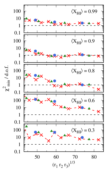
The dependence of the our 3PCF bias measurements on the global neutral fraction is displayed in Fig. 15 for all EoR models without RSD. In addition, for model A we show results from simulations with MMRRM RSDs. These measurements are derived from our largest scale bin with triangles which have on average a scale of Mpc. We find that the dependence of the linear and quadratic bias from all models is well fitted by first and second-order polynomials respectively. Requiring that is an unbiased tracer of the matter fluctuations at (i.e. and ) leads to the expressions
| (11) |
and
| (12) |
Fitting these expressions to the results from model A without RSD delivers , and . The bias measurements from the different models at fixed global neutral fractions show an overall agreement of , which lines up with the similarity of the 3PCF measurements from different models, shown in the right panel of Fig. 7. It is interesting to note, that the bias from model A with RSD is close to results derived without RSD, given the strong changes of the 21cm 3PCF amplitude due to RSD, which we saw in Fig. 10. This finding may be explained by the non-linear dependence of the 21cm 3PCF on linear bias, shown in equation (10) according to which small changes in the latter can cause strong changes in the former.
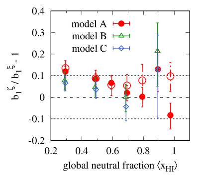
In Fig. 16 we show the relative deviations of the different measurements from Fig. 15 with respect to the corresponding measurements, derived from fits to the 21cm 2PCF in the range of Mpc. We thereby generalize the corresponding comparison from Fig. 14 to different EoR models and the case of model A with RSD. We find the linear bias from both statistics to agree at the level in all considered cases, which indicates that the bias measurements are physically meaningful. The fact that the measurements from the 2PCF and 3PCF also agree when RSDs are included in the simulations further suggests that the quadratic bias model may be useful for modeling observational data, albeit the meaning of the bias parameters is not clear and will change in the presence of RSD.

4.2 Direct measurements of the bias relation

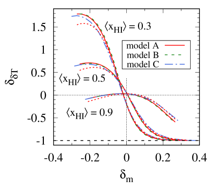
We now aim at a more direct test of the quadratic bias model, taking advantage of the fact that in the simulations we have access to both, the spatial fluctuations in the 21cm brightness temperature as well as those in the matter density. Having these quantities defined in smoothing volumes (i.e. grid cells) at different positions , enables us to directly measure the bias relation and verify how well it can be described by a deterministic function . Our particular interest lies thereby on testing how well this relation agrees with the quadratic bias model from equation (6), when using the bias parameters from the 3PCF measurements.
We show in Fig. 17 a scatter plot of the relation, for one realization of model A without RSD as grey dots, while each dot represents and measurements from one grid cell of the simulation. Results are shown for cells with side lengths of , and Mpc at redshifts with neutral fractions between and .
The results for Mpc grid cells show that, at very early times ( ), the 21cm brightness temperature fluctuations in most cells follow a roughly linear relation with respect to the matter density fluctuations, as expected from equation (5). A departure from this relation occurs for cells with high matter overdensities, where the 21cm brightness temperature is lower due to a higher fraction of ionized hydrogen. The effect becomes stronger at lower redshifts, as the reionization proceeds. At with , we already find a significant fraction of completely ionized cells with . The trend is apparent for all cell sizes, and provides an understanding of why the linear bias from the correlation function measurements changes its sign from positive to negative with decreasing redshift, as discussed in Section 4.1. The linear bias corresponds to the slope of the relation at . The results in Fig. 17 show clearly how this slope follows the trend expected from our previous measurements, while its value depends slightly on the cell size. For a more detailed comparison with the quadratic bias model predictions, we show in Fig. 17 the mean relation in bins of as black dots. We find this mean to be well approximated by fits to
| (13) |
at all considered redshifts and scales (red dashed lines in Fig. 17), where , and are free parameters. In addition to these fits, we show the prediction of the quadratic bias model with 3PCF bias parameters as solid blue lines. The 3PCF bias parameters were measured, using triangles with Mpc, covering the largest scales in our triangles sample (see Fig. 14). Comparing the quadratic bias model to the mean from the direct measurements in Fig. 17, we find a good agreement for large grid cells with Mpc side lengths. For cells with side Mpc side lengths, the quadratic model is a good approximation at , while clear deviations occur at the tails of the distribution. For the grid of Mpc cells, on which we measured most of the correlation functions (see Section 3.3), we find that the quadratic bias model differs strongly from the direct measurements for all values of . This result indicates that the residuals from the mean bias relation may not be random, but spatially correlated. They can hence affect the values at larger smoothing scales, and modify the measured bias parameters from the 3PCF fits. The agreement between the 3PCF bias prediction and the relation at large scales indicates, that both statistics are affected by the residuals in the same way, which is subject of our ongoing investigations.
In the previous Sections 4, we found that the 21cm 2PCF and 3PCF, as well as the bias parameters are almost independent of the EoR model at fixed volume weighted global neutral fractions (i.e. Fig. 4, 7 and 15), which suggests, that also the relation should only depend weakly on the EoR model at fixed . We test if this assumption holds, by comparing the mean relation for model A, B and C without RSD in Fig. 18 at values between and for a smoothing scale of Mpc. Our results line up with our previous findings, as we find very similar results from different EoR models. This implies, that the different 21cm statistics are almost entirely determined by the global neutral fraction. However, this result may be specific to the excursion set modeling, used by 21cmFAST. In addition to results without RSD, we show in Fig. 18 results with RSD from model A as red dotted lines. We find that at early times, when , RSDs enhance (decrease) the 21cm fluctuations in underdense (overdense) regions, while at later times the RSD effect in underdense regions is dominant. The latter finding may be understood from the fact that at later times less neutral gas in present overdense regions, which decreases the overall effect of RSDs on for high . As a result, the fraction of regions, which are affected by RSDs decreases with time, which lines up with the lower impact of RSDs on the 21cm correlation functions at late times, which we found in Fig. 6 and 10. However, a conclusive interpretation of these results requires further investigations.
5 Summary and Conclusions
We studied 2PCF and 3PCF of the 21cm brightness temperature during the epoch of reionization. The goal of our study was to characterize the 21cm 2PCF and, for the first time, the 21cm 3PCF in configuration space for different redshifts, scales and triangle shapes, using measurements in simulations. Based on these measurements we tested how well these 21cm correlation functions can be described by the local quadratic bias model, which has been commonly employed for relating the 2PCF and 3PCF of galaxies and halos to the corresponding statistics of the underlying dark matter density field.
Our simulations were produced by the semi-numerical code 21cmFAST (Mesinger et al., 2011), using three different combinations of EoR model parameters, to which we refer to as model A, B and C, as summarized in Table 1. For each parameter combination we generated realizations of the 21cm brightness temperature and the underlying matter density field with different random initial conditions. Each set of simulations covers a total volume of up to , providing small errors as well as error covariance estimates for our 2PCF and 3PCF measurements, which allows for a detailed comparison with the bias model predictions. Redshift space distortions (RSDs) are neglected in the main part of our analysis, which we discuss in the following, to simplify the interpretation of our results. However, for our fiducial model A, we investigated how the 21cm correlations and the corresponding bias measurements are affected by RSDs, which is briefly discussed towards the end of this section.
Our 21cm 2PCF measurements present a strong redshift evolution, with an amplitude change of orders of magnitude for neutral fractions in the range () for model A, which demonstrates the high sensitivity of the 21cm 2PCF to the state of reionization. This redshift evolution is also highly sensitive to the EoR model parameters, while results from different parameter combinations show a percent level agreement at all considered scales when compared at fixed global neutral fractions (Fig. 4). The quadratic expansion of the local bias model in equation (6) predicts that the matter and 21cm 2PCF are related to each other by the scale independent linear bias factor at leading order. We show in Fig. 5 that this prediction can describe the measurements at scales between and Mpc with () accuracy for (). This means that the impact of the reionization on the large-scale 21cm 2PCF can be well characterized by a single parameter, which limits the constraining power of this statistics for reionization models. Strong deviations from the leading order 2PCF bias model occur at scales of Mpc, which corresponds roughly to the typical size of ionized regions in our simulation (Fig. 3). This finding indicates that patchy reionization needs to be taken into account for a detailed modeling of the 21cm 2PCF at small scales and late times, as it has been discussed in the literature (e.g. Furlanetto et al., 2004).
Our measurements of the 21cm 3PCF show a strong dependence on the triangle opening angle, as well as on the overall length scale defined as (see e.g. Fig. 11). For a fixed triangle shape, we find a stronger change of the amplitude than for the 2PCF by up to four orders of magnitude in the considered redshift range (Fig. 9). The dependence on the opening angle shows that the 3PCF does not only probe the scale dependence of the 21cm fluctuations, but also their morphology. It therefore provides access to additional information in the 21cm signal besides its non-Gaussianity, to which the 2PCF is not sensitive. As for the 2PCF, we find a strong dependence of the 21cm 3PCF on the EoR model parameters at fixed redshifts, while results from different parameter combinations agree at the level (Fig. 7) at fixed global neutral fractions.
The leading-order approximation of 21cm 3PCF, based on the bias model from equation (10), delivers fits which are in agreement with our measurements (Fig. 11) for triangles with Mpc. This result indicates a good performance of the bias model, given our small measurements errors. A notable small scale feature of our 3PCF measurements, which is not described by the bias model, is the increase of the amplitude at the smallest scales at early times ( , Fig. 9). Such an increase has also been reported by Majumdar et al. (2018) for bispectrum measurements in simulations, as well model predictions, based on randomly distributed ionized bubbles.
The dependence of our best fit bias parameters on the chosen triangle scale range, shown in Fig. 14, is within the expected uncertainty for . At this scale dependence becomes more significant, indicating a breakdown of the leading order 3PCF bias model at late times of reioinization, which we already noticed in the 2PCF analysis (Fig. 5). The linear bias from the 3PCF is compared to the results from the 2PCF in Fig. 16. The comparison reveals a agreement for all EoR parameter combinations in the considered redshift range (with ), when the analysis is restricted to large triangles with Mpc. This result is consistent with the aforementioned inaccuracy of the linear bias model for the 2PCF at large scales.
Our comparison with results from approximate N-body simulations based on the COLA method, shown in Fig. 4, 8 and 9, revealed that our main results for the correlations of the matter and 21cm fields are only weakly affected by the usage of the Zel’dovich approximation at large scales. We therefore consider our conclusions drawn from these measurements to be robust in this regard. Note that this would not be the case at small scales and low redshifts (Scoccimarro, 1997; Leclercq et al., 2013). The good agreement between the linear bias from the two- and three-point statistics further indicates that the quadratic bias model is physically meaningful, in particular at large scales and early times. The simple polynomial relations between the linear and quadratic bias with respect to the global neutral fraction, shown in Fig. 15, further indicate that there may be a simple physical interpretation of the bias parameters (see also McQuinn & D’Aloisio, 2018).
Up to this point we tested the quadratic bias model for the assumed deterministic relation via its leading order prediction for the 2PCF and 3PCF. In the final step of our analysis, we conducted a more direct test of the model, by comparing its predicted relation to direct measurements of this relation in the simulations (Fig. 17). For this comparison, we employ the linear and quadratic bias parameters, measured from the 3PCF at large scales. We find strong deviations between the bias model prediction and the direct average value of in bins of when using small smoothing scales of Mpc for the direct measurements. However, for large smoothing scales of Mpc, we find very good agreement in the considered redshift range. Another interesting finding is that the average relation is well approximated by the analytic expression, given by equation (13). The physical interpretation of this expression may provide the aforementioned interpretation of the bias parameters and is the subject of our followup work.
The results discussed above refer to our simulations without RSDs. We included the latter to our simulations with EoR model A using a simplistic RSD model, which was implemented in 21cmFAST. We compared these results to those based on the physically better motivated MMRRM model for RSDs from Mao et al. (2012). For both RSD models we find a stronger impact of RSDs on the 21cm 2PCF at early times of reionization (Fig. 6), confirming results from the literature for the 21cm power spectrum (e.g. McQuinn et al., 2006; Mesinger & Furlanetto, 2007). We find the same trend for the 21cm 3PCF, while in that case the change of the amplitude is overall stronger than for the 2PCF and highly dependent on the scale, as well as on the triangle opening angle (Fig. 10). For both statistics the impact of RSDs from the MMRRM model are significantly stronger than predicted by the simplistic model from 21cmFAST, in particular at late times with low global neutral fractions. It is interesting to note that the bias parameters are only weakly affected by RSDs, despite of the strong change in of the correlations functions. This finding may result from the non-linear relation between the linear bias and correlation functions, given by equation (8) and (10).
Overall our results show that the quadratic bias model provides a consistent description of the 21cm 2PCF and 3PCF in 21cmFAST simulations on scales larger than Mpc at early times of the reionization with . It further describes the well at large smoothing scales of Mpc. The latter finding suggests that the linear and quadratic bias parameter measurements from the 21cm 3PCF can provide insights to the process leading to the reionization from upcoming 21cm observations. In principle, the linear and quadratic bias parameters, and , depend on the underlying model that predicts both global reionization history and the clustering and morphology of ionized regions. Measurements of the 21cm 3PCF in upcoming radio observations, therefore, can improve constraints on astrophysical processes driving reionization upon those from the 2PCF. We further find that a detailed interpretation of the bias parameters from the observed 21cm 3PCF in three dimension 21cm mapping further requires an understanding of how the 21cm 3PCF is affected by RSDs. A general limitation for our approach is given by the fact that our analysis is based on fluctuations of the brightness temperature around the global mean, i.e. the monopole of the 21cm signal. Nevertheless, the 21cm mean signal cannot be observed with radio interferometers such as SKA and HERA, and would therefore need to be obtained from single antenna experiments.
Recently Beane & Lidz (2018) found that the quadratic bias model also provides reasonable fits to measurements of the three-point cross-bispectrum between maps of the 21cm brightness temperature and the CII emission line intensity in simulations. This work showed on one hand, that the bias model still holds when being applied on the 21cm signal, instead of its fluctuations. This can be expected, given that the underlying assumption of a deterministic bias function is not restricted to a given definition of the observed quantity, as long as deviations around the expansion point are sufficiently small on average. On the other hand, their work demonstrated the applicability of the bias modeling in Fourier space, which is more closely related to future observational data sets. However, the configuration space analysis, on which the present work is based, simplifies the physical interpretation of the results, such as the aforementioned impact of residuals around the mean bias relation on the clustering. The latter may be important to understand shortcomings of the bias model revealed in this work, in particular at small scales and late times of reionization. An improvement of the bias model might require further investigation of such residuals as well as an expansion of the 21cm 2PCF and 3PCF beyond the leading order. Such improvements were recently investigated by McQuinn & D’Aloisio (2018), who found that adding a dependence on the wave number and an effective bubble size parameter to the quadratic terms in the bias expansion provides better fits to the 21cm power spectrum at late times of reionization.
Acknowledgments
YM and HJM were supported in part by the National Key Basic Research and Development Program of China (No.2018YFA0404502, No.2018YFA0404503), and by the NSFC-ISF joint research program (NSFC Grant No.11761141012), and the National Natural Science Foundation of China (“NSFC”, Grant No.11821303). YM was also supported in part by the NSFC (Grant No.11673014, 11543006), by the National Key Program for Science and Technology Research and Development of China (No.2017YFB0203302), by the Chinese National Thousand Youth Talents Program, and by the Opening Project of Key Laboratory of Computational Astrophysics, National Astronomical Observatories, Chinese Academy of Sciences. KH was supported in part by the NSFC (Grant No.11750110419), by the China Postdoctoral Science Foundation, and the International Postdoctoral Fellowship from the Ministry of Education and the State Administration of Foreign Experts Affairs of China. HJM was also supported in part by the NSFC (Grant No.11673015,11733004,11761131004) and NSF AST-1517528. BDW acknowledges support from the Simons Foundation.
References
- Baldauf et al. (2012) Baldauf T., Seljak U., Desjacques V., McDonald P., 2012, Phys. Rev. D, 86, 083540
- Barkana & Loeb (2001) Barkana R., Loeb A., 2001, Phys. Rept., 349, 125
- Barriga & Gaztañaga (2002) Barriga J., Gaztañaga E., 2002, MNRAS, 333, 443
- Beane & Lidz (2018) Beane A., Lidz A., 2018, ApJ, 867, 26
- Bernardeau et al. (2002) Bernardeau F., Colombi S., Gaztañaga E., Scoccimarro R., 2002, Phys. Rept., 367, 1
- Bharadwaj & Pandey (2005) Bharadwaj S., Pandey S. K., 2005, MNRAS, 358, 968
- Bryan & Norman (1998) Bryan G. L., Norman M. L., 1998, ApJ, 495, 80
- Chan et al. (2012) Chan K. C., Scoccimarro R., Sheth R. K., 2012, Phys. Rev. D, 85, 083509
- Eisenstein & Hu (1998) Eisenstein D. J., Hu W., 1998, ApJ, 496, 605
- Field (1958) Field G. B., 1958, Proceedings of the IRE, 46, 240
- Fry & Gaztanaga (1993) Fry J. N., Gaztanaga E., 1993, ApJ, 413, 447
- Furlanetto (2006) Furlanetto S. R., 2006, MNRAS, 371, 867
- Furlanetto et al. (2004) Furlanetto S. R., Zaldarriaga M., Hernquist L., 2004, ApJ, 613, 1
- Furlanetto et al. (2006) Furlanetto S. R., Oh S. P., Briggs F. H., 2006, Phys. Rept., 433, 181
- Gaztañaga & Scoccimarro (2005) Gaztañaga E., Scoccimarro R., 2005, MNRAS, 361, 824
- Hartlap et al. (2007) Hartlap J., Simon P., Schneider P., 2007, A&A, 464, 399
- Hoffmann et al. (2018) Hoffmann K., Gaztañaga E., Scoccimarro R., Crocce M., 2018, MNRAS, 476, 814
- Howlett et al. (2015) Howlett C., Manera M., Percival W. J., 2015, Astronomy and Computing, 12, 109
- Leclercq et al. (2013) Leclercq F., Jasche J., Gil-Marín H., Wandelt B., 2013, Journal of Cosmology and Astroparticle Physics, 11, 048
- Lidz et al. (2007) Lidz A., Zahn O., McQuinn M., Zaldarriaga M., Dutta S., Hernquist L., 2007, ApJ, 659, 865
- Liu & Parsons (2016) Liu A., Parsons A. R., 2016, MNRAS, 457, 1864
- Majumdar et al. (2018) Majumdar S., Pritchard J. R., Mondal R., Watkinson C. A., Bharadwaj S., Mellema G., 2018, MNRAS, 476, 4007
- Mao et al. (2012) Mao Y., Shapiro P. R., Mellema G., Iliev I. T., Koda J., Ahn K., 2012, MNRAS, 422, 926
- McQuinn & D’Aloisio (2018) McQuinn M., D’Aloisio A., 2018, Journal of Cosmology and Astro-Particle Physics, 2018, 016
- McQuinn et al. (2006) McQuinn M., Zahn O., Zaldarriaga M., Hernquist L., Furlanetto S. R., 2006, ApJ, 653, 815
- Mesinger & Furlanetto (2007) Mesinger A., Furlanetto S., 2007, ApJ, 669, 663
- Mesinger et al. (2011) Mesinger A., Furlanetto S., Cen R., 2011, MNRAS, 411, 955
- Pober et al. (2014) Pober J. C., et al., 2014, ApJ, 782, 66
- Pritchard & Furlanetto (2007) Pritchard J. R., Furlanetto S. R., 2007, MNRAS, 376, 1680
- Pritchard & Loeb (2012) Pritchard J. R., Loeb A., 2012, Reports on Progress in Physics, 75, 086901
- Raste & Sethi (2018) Raste J., Sethi S., 2018, ApJ, 860, 55
- Schmit & Pritchard (2018) Schmit C. J., Pritchard J. R., 2018, MNRAS, 475, 1213
- Scoccimarro (1997) Scoccimarro R., 1997, ApJ, 487, 1
- Shimabukuro et al. (2016) Shimabukuro H., Yoshiura S., Takahashi K., Yokoyama S., Ichiki K., 2016, MNRAS, 458, 3003
- Shimabukuro et al. (2017) Shimabukuro H., Yoshiura S., Takahashi K., Yokoyama S., Ichiki K., 2017, MNRAS, 468, 1542
- Sokasian et al. (2004) Sokasian A., Yoshida N., Abel T., Hernquist L., Springel V., 2004, MNRAS, 350, 47
- Tassev et al. (2013) Tassev S., Zaldarriaga M., Eisenstein D. J., 2013, Journal of Cosmology and Astro-Particle Physics, 2013, 036
- Zaldarriaga et al. (2004) Zaldarriaga M., Furlanetto S. R., Hernquist L., 2004, ApJ, 608, 622
Appendix A Effect of simulation Box size on 21cm 2PCF measurements
The size of the simulation box determines the wavelength of the largest mode, in the matter density field of our simulation. The box size can therefore affect the matter and 21cm correlation functions, which we measure in the simulations on large scales.
To test how strongly our 21cm 2PCF measurements are affected by the chosen box size we generate realizations, each with twice the side length (i.e. Mpc) than for the realizations (with the side length Mpc) used in our analysis. In the top panel of Fig. 19 we compare the 21cm 2PCF measurements for both simulation boxes at the redshift ( ). Our results show that our chosen box size affects the 2PCF measurements on large scales Mpc, while results at smaller scales are not significantly affected.

Appendix B Relative deviations of 21cm 3PCF fits from measurements
We test the fitting performance of the bias model here by showing the relative deviations between fits and measurements at different triangle scales and global neutral fractions in Fig. 20. This test is complementary to the test of the significance of deviations between fits and measurements shown in Fig. 11. In the latter figure we find a better performance of the bias model at large scales. With Fig. 20 we point out, that the large relative deviations can occur at small as well as on large scales. Since the 3PCF errors increase with scales due to fewer modes in our simulation volume, large-scale deviations are less significant.

Appendix C Covariances and fitting
We fit the bias model predictions for the 21cm 2PCF and 3PCF (equation (8) and (10) respectively) to the corresponding measurements by a minimization. We therefore explore the parameter space, searching for the minimum of
| (14) |
where . The mean measurements for a certain scale or triangle over the realizations are denoted as , while are the corresponding predictions. The variance of is given by . The factor accounts for the fact that we are interested in the errors on the mean measurements, rather than those on measurements from individual realizations. The normalized covariance matrix is hence given by
| (15) |
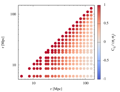
with . We show examples of our measurements for the 2PCF and 3PCF in Fig. 21 and 22, respectively. In both cases, the covariance matrix has strong off-diagonal elements, in particular at small scales. This indicates that knowledge of the covariance is essential for constraining theory models from 21cm 2PCF and 3PCF measurements in future observations. Based on these covariance measurements, our fits are performed for measurements from different scales or triangles, to ensure that the covariance is invertible (Hartlap et al., 2007).
We find that 3PCF fits based on equation (14) can be very sensitive to small changes in the selected triangle sample, which may be caused by noise in our covariance estimation from the only realizations. To reduce this noise, we follow Gaztañaga & Scoccimarro (2005) by performing a Singular Value Decomposition of the covariance (hereafter referred to as SVD), i.e.
| (16) |
The diagonal matrix consists of the singular values (“SVs”), while the corresponding normalized modes form the matrix . The modes associated to the largest SVs may be understood analogously to eigenvectors. The expression from equation (14) can now be approximated by writing it in terms of the most dominant modes
| (17) |
The elements of the vector correspond to the quantity , which appears in equation (14). Fig. 23 shows that is typically dominated only by a few modes. Assuming that the modes with the lowest SVs can be associated with measurement noise, we use only SVs with values larger than the sampling error estimate (i.e. ) for our computation, as suggested by Gaztañaga & Scoccimarro (2005). The number of selected modes is hence the degree of freedom in our estimation, i.e. d.o.f. = . Note that the description above matches in various parts of Section 2.4 in Hoffmann et al. (2018), who did a similar analysis for the halo 3PCF.