Yes, but Did It Work?: Evaluating Variational Inference

Supplement to “Yes, but Did It Work?: Evaluating Variational Inference”

Abstract

While it’s always possible to compute a variational approximation to a posterior distribution, it can be difficult to discover problems with this approximation. We propose two diagnostic algorithms to alleviate this problem. The Pareto-smoothed importance sampling (PSIS) diagnostic gives a goodness of fit measurement for joint distributions, while simultaneously improving the error in the estimate. The variational simulation-based calibration (VSBC) assesses the average performance of point estimates.

1 Introduction

Variational Inference (VI), including a large family of posterior approximation methods like stochastic VI (Hoffman et al. 2013), black-box VI (Ranganath et al. 2014), automatic differentiation VI (ADVI, Kucukelbir et al. 2017), and many other variants, has emerged as a widely-used method for scalable Bayesian inference. These methods come with few theoretical guarantees and it’s difficult to assess how well the computed variational posterior approximates the true posterior.

Instead of computing expectations or sampling draws from the posterior $p(\theta\mid y)$, variational inference fixes a family of approximate densities $\mathcal{Q}$, and finds the member $q^{*}$ minimizing the Kullback-Leibler (KL) divergence to the true posterior: $\operatorname{\mathrm{KL}}\left(q(\theta),p(\theta\mid y)\right).$ This is equivalent to maximizing the evidence lower bound (ELBO):

$$\quad\mathrm{ELBO}(q)=\int_{\Theta}\left(\log p(\theta,y)-\log q(\theta)\right)q(\theta)d\theta.$$ (1)

There are many situations where the VI approximation is flawed. This can be due to the slow convergence of the optimization problem, the inability of the approximation family to capture the true posterior, the asymmetry of the true distribution, the fact that the direction of the KL divergence under-penalizes approximation with too-light tails, or all these reasons. We need a diagnostic algorithm to test whether the VI approximation is useful.

There are two levels of diagnostics for variational inference. First the convergence test should be able to tell if the objective function has converged to a local optimum. When the optimization problem (1) is solved through stochastic gradient descent (SGD), the convergence can be assessed by monitoring the running average of ELBO changes. Researchers have introduced many convergence tests based on the asymptotic property of stochastic approximations (e.g., Sielken, 1973; Stroup & Braun, 1982; Pflug, 1990; Wada & Fujisaki, 2015; Chee & Toulis, 2017). Alternatively, Blei et al. (2017) suggest monitoring the expected log predictive density by holding out an independent test dataset. After convergence, the optimum is still an approximation to the truth. This paper is focusing on the second level of VI diagnostics whether the variational posterior $q^{*}(\theta)$ is close enough to the true posterior $p(\theta|y)$ to be used in its place.

Purely relying on the objective function or the equivalent ELBO does not solve the problem. An unknown multiplicative constant exists in $p(\theta,y)\propto p(\theta\mid y)$ that changes with reparametrization, making it meaningless to compare ELBO across two approximations. Moreover, the ELBO is a quantity on an uninterpretable scale, that is it’s not clear at what value of the ELBO we can begin to trust the variational posterior. This makes it next to useless as a method to assess how well the variational inference has fit.

In this paper we propose two diagnostic methods that assess, respectively, the quality of the entire variational posterior for a particular data set, and the average bias of a point estimate produced under correct model specification.

The first method is based on generalized Pareto distribution diagnostics used to assess the quality of a importance sampling proposal distribution in Pareto smoothed importance sampling (PSIS, Vehtari et al., 2017). The benefit of PSIS diagnostics is two-fold. First, we can tell the discrepancy between the approximate and the true distribution by the estimated continuous $\hat{k}$ value. When it is larger than a pre-specified threshold, users should be alert of the limitation of current variational inference computation and consider further tuning it or turn to exact sampling like Markov chain Monte Carlo (MCMC). Second, in the case when $\hat{k}$ is small, the fast convergence rate of the importance-weighted Monte Carlo integration guarantees a better estimation accuracy. In such sense, the PSIS diagnostics could also be viewed as a post-adjustment for VI approximations. Unlike the second-order correction Giordano et al. (2017), which relies on an un-testable unbiasedness assumption, we make diagnostics and adjustment at the same time.

The second diagnostic considers only the quality of the median of the variational posterior as a point estimate (in Gaussian mean-field VI this corresponds to the modal estimate). This diagnostic assesses the average behavior of the point estimate under data from the model and can indicate when a systemic bias is present. The magnitude of that bias can be monitored while computing the diagnostic. This diagnostic can also assess the average calibration of univariate functionals of the parameters, revealing if the posterior is under-dispersed, over-dispersed, or biased. This diagnostic could be used as a partial justification for using the second-order correction of Giordano et al. (2017).

2 Is the Joint Distribution Good Enough?

If we can draw a sample $(\theta_{1},\dots,\theta_{S})$ from $p(\theta|y)$, the expectation of any integrable function $\operatorname{\mathrm{E}}_{p}[h(\theta)]$ can be estimated by Monte Carlo integration: $\sum_{s=1}^{S}h(\theta_{s})/S\!\!\!\xrightarrow[]{\enskip S\to\infty\enskip}\!\!\!\operatorname{\mathrm{E}}_{p}\left[h(\theta)\right].$ Alternatively, given samples $(\theta_{1},\dots,\theta_{S})$ from a proposal distribution $q(\theta)$, the importance sampling (IS) estimate is $\left({\sum_{s=1}^{S}h(\theta_{s})r_{s}}\right)/{\sum_{s=1}^{S}r_{s}}$, where the importance ratios $r_{s}$ are defined as

$$r_{s}=\frac{p(\theta_{s},y)}{q(\theta_{s})}.$$ (2)

In general, with a sample $(\theta_{1},\dots,\theta_{S})$ drawn from the variational posterior $q(\theta)$, we consider a family of estimates with the form

$$E_{p}[h(\theta)]\approx\frac{\sum_{s=1}^{S}h(\theta_{s})w_{s}}{\sum_{s=1}^{S}w_{s}},$$ (3)

which contains two extreme cases:

1. When $w_{s}\equiv 1$, estimate (3) becomes the plain VI estimate that is we completely trust the VI approximation. In general, this will be biased to an unknown extent and inconsistent. However, this estimator has small variance.

2. When $w_{s}=r_{s}$, (3) becomes importance sampling. The strong law of large numbers ensures it is consistent as $S\to\infty$, and with small $O(1/S)$ bias due to self-normalization. But the IS estimate may have a large or infinite variance.

There are two questions to be answered. First, can we find a better bias-variance trade-off than both plain VI and IS?

Second, VI approximation $q(\theta)$ is not designed for an optimal IS proposal, for it has a lighter tail than $p(\theta|y)$ as a result of entropy penalization, which lead to a heavy right tail of $r_{s}$. A few large-valued $r_{s}$ dominates the summation, bringing in large uncertainty. But does the finite sample performance of IS or stabilized IS contain the information about the dispensary measure between $q(\theta)$ and $p(\theta|y)$?

2.1 Pareto Smoothed Importance Sampling

The solution to the first question is the Pareto smoothed importance sampling (PSIS). We give a brief review, and more details can be found in Vehtari et al. (2017).

A generalized Pareto distribution with shape parameter $k$ and location-scale parameter $(\mu,\tau)$ has the density

$$p(y|\mu,\sigma,k)=\left\{\begin{aligned} &\frac{1}{\sigma}\left(1+k\left(\frac{y-\mu}{\sigma}\right)\right)^{-\frac{1}{k}-1},&k\neq 0.\\ &\frac{1}{\sigma}\exp\left(\frac{y-\mu}{\sigma}\right),&k=0.\\ \end{aligned}\right.$$

PSIS stabilizes importance ratios by fitting a generalized Pareto distribution using the largest $M$ samples of $r_{i}$, where $M$ is empirically set as $\min(S/5,3\sqrt{S})$. It then reports the estimated shape parameter $\hat{k}$ and replaces the $M$ largest $r_{s}$ by their expected value under the fitted generalized Pareto distribution. The other importance weights remain unchanged. We further truncate all weights at the raw weight maximum $\max(r_{s})$. The resulted smoothed weights are denoted by $w_{s}$, based on which a lower variance estimation can be calculated through (3).

Pareto smoothed importance sampling can be considered as Bayesian version of importance sampling with prior on the largest importance ratios. It has smaller mean square errors than plain IS and truncated-IS (Ionides, 2008).

2.2 Using PSIS as a Diagnostic Tool

The fitted shape parameter $\hat{k}$, turns out to provide the desired diagnostic measurement between the true posterior $p(\theta|y)$ and the VI approximation $q(\theta)$. A generalized Pareto distribution with shape $k$ has finite moments up to order $1/k$, thus any positive $\hat{k}$ value can be viewed as an estimate to

$$k=\inf\left\{k^{\prime}>0:E_{q}\left(\frac{p(\theta|y)}{q(\theta)}\right)^{\frac{1}{k^{\prime}}}<\infty\right\}.$$ (4)

$\hat{k}$ is invariant under any constant multiplication of $p$ or $q$, which explains why we can suppress the marginal likelihood (normalizing constant) $p(y)$ and replace the intractable $p(\theta|y)$ with $p(\theta,y)$ in (2).

After log transformation, (4) can be interpreted as Rényi divergence (Rényi et al., 1961) with order $\alpha$ between $p(\theta|y)$ and $q(\theta)$:

$$k=\inf\left\{k^{\prime}>0:D_{\frac{1}{k^{\prime}}}\left(p||q\right)<\infty\right\},$$

$$\mathrm{where}\> D_{\alpha}\left(p||q\right)=\frac{1}{\alpha-1}\log\int_{\Theta}p(\theta)^{\alpha}q(\theta)^{1-\alpha}d\theta.$$

It is well-defined since Rényi divergence is monotonic increasing on order $\alpha$. Particularly, when $k>0.5$, the $\chi^{2}$ divergence $\chi(p||q)$, becomes infinite, and when $k>1$, $D_{1}(p||q)=\operatorname{\mathrm{KL}}(p,q)=\infty$, indicating a disastrous VI approximation, despite the fact that $\operatorname{\mathrm{KL}}(q,p)$ is always minimized among the variational family. The connection to Rényi divergence holds when $k>0$. When $k<0$, it predicts the importance ratios are bounded from above.

This also illustrates the advantage of a continuous $\hat{k}$ estimate in our approach over only testing the existence of second moment of $E_{q}(q/p)^{2}$ (Epifani et al., 2008; Koopman et al., 2009) – it indicates if the Rényi divergence between $q$ and $p$ is finite for all continuous order $\alpha>0$.

Meanwhile, the shape parameter $k$ determines the finite sample convergence rate of both IS and PSIS adjusted estimate. Geweke (1989) shows when $\operatorname{\mathrm{E}}_{q}[r(\theta)^{2}]<\infty$ and $\operatorname{\mathrm{E}}_{q}[\bigl{(}r(\theta)h(\theta)\bigr{)}^{2}]<\infty$ hold (both conditions can be tested by $\hat{k}$ in our approach), the central limit theorem guarantees the square root convergence rate. Furthermore, when $k<1/3$, then the Berry-Essen theorem states faster convergence rate to normality (Chen et al., 2004). Cortes et al. (2010) and Cortes et al. (2013) also link the finite sample convergence rate of IS with the number of existing moments of importance ratios.

PSIS has smaller estimation error than the plain VI estimate, which we will experimentally verify this in Section 4. A large $\hat{k}$ indicates the failure of finite sample PSIS, so it further indicates the large estimation error of VI approximation. Therefore, even when the researchers’ primary goal is not to use variational approximation $q$ as an PSIS proposal, they should be alert by a large $\hat{k}$ which tells the discrepancy between the VI approximation result and the true posterior.

According to empirical study in Vehtari et al. (2017), we set the threshold of $\hat{k}$ as follows.

• If $\hat{k}<0.5$, we can invoke the central limit theorem to suggest PSIS has a fast convergence rate. We conclude the variational approximation $q$ is close enough to the true density. We recommend further using PSIS to adjust the estimator (3) and calculate other divergence measures.

• If $0.5<\hat{k}<0.7$, we still observe practically useful finite sample convergence rates and acceptable Monte Carlo error for PSIS. It indicates the variational approximation $q$ is not perfect but still useful. Again, we recommend PSIS to shrink errors.

• If $\hat{k}>0.7$, the PSIS convergence rate becomes impractically slow, leading to a large mean square error, and a even larger error for plain VI estimate. We should consider tuning the variational methods (e.g., re-parametrization, increase iteration times, increase mini-batch size, decrease learning rate, et.al.,) or turning to exact MCMC. Theoretically $k$ is always smaller than 1, for $E_{q}\left[{p(\theta|y)}/{q(\theta)}\right]=p(y)<\infty$, while in practice finite sample estimate $\hat{k}$ may be larger than 1, which indicates even worse finite sample performance.

The proposed diagnostic method is summarized in Algorithm 1.

Algorithm 1 PSIS diagnostic

1:  Input: the joint density function $p(\theta,y)$; number of posterior samples $S$; number of tail samples $M$.

2:  Run variational inference to $p(\theta|y)$, obtain VI approximation $q(\theta)$;

3:  Sample $(\theta_{s},s=1,\dots,S)$ from $q(\theta)$;

4:  Calculate the importance ratio $r_{s}=p(\theta_{s},y)/q(\theta_{s})$;

5:  Fit generalized Pareto distribution to the $M$ largest $r_{s}$;

6:  Report the shape parameter $\hat{k}$;

7:  if  $\hat{k}<0.7$  then

8:     Conclude VI approximation $q(\theta)$ is close enough to the unknown truth $p(\theta|y)$;

9:     Recommend further shrinking errors by PSIS.

10:  else

11:     Warn users that the VI approximation is not reliable.

12:  end if

2.3 Invariance Under Re-Parametrization

Re-parametrization is common in variational inference. Particularly, the reparameterization trick (Rezende et al., 2014) rewrites the objective function to make gradient calculation easier in Monte Carlo integrations.

A nice property of PSIS diagnostics is that the $\hat{k}$ quantity is invariant under any re-parametrization. Suppose $\xi$ = $T(\theta)$ is a smooth transformation, then the density ratio of $\xi$ under the target $p$ and the proposal $q$ does not change:

$$\frac{p(\xi)}{q(\xi)}=\frac{p\left(T^{-1}(\xi)\right)|\mathrm{det}J_{\xi}T^{-1}(\xi)|}{q\left(T^{-1}(\xi)\right)|\mathrm{det}J_{\xi}T^{-1}(\xi)|}=\frac{p\left(\theta\right)}{q(\theta)}$$

Therefore, ${p(\xi)}/{q(\xi)}$ and ${p(\theta)}/{q(\theta)}$ have the same distribution under $q$, making it free to choose any convenient parametrization form when calculating $\hat{k}$.

However, if the re-parametrization changes the approximation family, then it will change the computation result, and PSIS diagnostics will change accordingly. Finding the optimal parametrization form, such that the re-parametrized posterior distribution lives exactly in the approximation family

$$p(T(\xi))=p\left(T^{-1}(\xi)\right)|J_{\xi}T^{-1}(\xi)|\in\mathcal{Q},$$

can be as hard as finding the true posterior. The PSIS diagnostic can guide the choice of re-parametrization by simply comparing the $\hat{k}$ quantities of any parametrization. Section 4.3 provides a practical example.

2.4 Marginal PSIS Diagnostics Do Not Work

As dimension increases, the VI posterior tends to be further away from the truth, due to the limitation of approximation families. As a result, $k$ increases, indicating inefficiency of importance sampling. This is not the drawback of PSIS diagnostics. Indeed, when the focus is the joint distribution, such behaviour accurately reflects the quality of the variational approximation to the joint posterior.

Denoting the one-dimensional true and approximate marginal density of the $i$-th coordinate $\theta_{i}$ as $p(\theta_{i}|y)$ and $q(\theta_{i})$, the marginal ${k}$ for $\theta_{i}$ can be defined as

$$k_{i}=\inf\left\{0<k^{\prime}<1:\operatorname{\mathrm{E}}_{q}\left(\frac{p(\theta_{i}|y)}{q(\theta_{i})}\right)^{\frac{1}{k^{\prime}}}<\infty\right\}.$$

The marginal $k_{i}$ is never larger (and usually smaller) than the joint ${k}$ in (4).

Proposition 1.

For any two distributions $p$ and $q$ with support $\Theta$ and the margin index $i$, if there is a number $\alpha>1$ satisfying $E_{q}\left(p(\theta)/q(\theta)\right)^{\alpha}<\infty$, then $E_{q}\left(p(\theta_{i})/q(\theta_{i})\right)^{\alpha}<\infty$.

Proposition 1 demonstrates why the importance sampling is usually inefficient in high dimensional sample space, in that the joint estimation is “worse” than any of the marginal estimation.

Should we extend the PSIS diagnostics to marginal distributions? We find two reasons why the marginal PSIS diagnostics can be misleading. Firstly, unlike the easy access to the unnormalized joint posterior distribution $p(\theta,y)$, the true marginal posterior density $p(\theta_{i}|y)$ is typically unknown, otherwise one can conduct one-dimensional sampling easily to obtain the the marginal samples. Secondly, a smaller $\hat{k}_{i}$ does not necessary guarantee a well-performed marginal estimation. The marginal approximations in variational inference can both over-estimate and under-estimate the tail thickness of one-dimensional distributions, the latter situation gives rise to a smaller $\hat{k}_{i}$. Section 4.3 gives an example, where the marginal approximations with extremely small marginal ${k}$ have large estimation errors. This does not happen in the joint case as the direction of the Kullback-Leibler divergence $q^{*}(\theta)$ strongly penalizes too-heavy tails, which makes it unlikely that the tails of the variational posterior are significantly heavier than the tails of the true posterior.

3 Assessing the Average Performance of the Point Estimate

The proposed PSIS diagnostic assesses the quality of the VI approximation to the full posterior distribution. It is often observed that while the VI posterior may be a poor approximation to the full posterior, point estimates that are derived from it may still have good statistical properties. In this section, we propose a new method for assessing the calibration of the center of a VI posterior.

3.1 The Variational Simulation-Based Calibration (VSBC) Diagnostic

This diagnostic is based on the proposal of Cook et al. (2006) for validating general statistical software. They noted that if $\theta^{(0)}\sim p(\theta)$ and $y\sim p(y\mid\theta^{(0)})$, then

$${\Pr}_{(y,\theta^{(0)})}\left({\Pr}_{\theta\mid y}(\theta<\theta^{(0)})\leq\cdot)\right)=\text{Unif}_{[0,1]}([0,\cdot]).$$

To use the observation of Cook et al. (2006) to assess the performance of a VI point estimate, we propose the following procedure. Simulate $M>1$ data sets $\{{y}_{j}\}_{j=1}^{M}$ as follows: Simulate $\theta_{j}^{(0)}\sim p(\theta)$ and then simulate ${y}_{(j)}\sim p(y\mid\theta_{j}^{(0)})$, where ${y}_{(j)}$ has the same dimension as $y$. For each of these data sets, construct a variational approximation to $p(\theta\mid y_{j})$ and compute the marginal calibration probabilities $p_{ij}=\Pr_{\theta\mid y_{(j)}}\left(\theta_{i}\leq[\theta_{j}^{(0)}]_{i}\right)$.

To apply the full procedure of Cook et al. (2006), we would need to test $\operatorname{dim}(\theta)$ histograms for uniformity, however this would be too stringent a check as, like our PSIS diagnostic, this test is only passed if the variational posterior is a good approximation to the true posterior. Instead, we follow an observation of Anderson (1996) from the probabilistic forecasting validation literature and note that asymmetry in the histogram for $p_{i:}$ indicates bias in the variational approximation to the marginal posterior $\theta_{i}\mid y$.

The VSBC diagnostic tests for symmetry of the marginal calibration probabilities around $0.5$ and either by visual inspection of the histogram or by using a Kolmogorov-Smirnov (KS) test to evaluate whether $p_{i:}$ and $1-p_{i:}$ have the same distribution. When $\theta$ is a high-dimensional parameter, it is important to interpret the results of any hypothesis tests through a multiple testing lens.

Algorithm 2 VSBC marginal diagnostics

1:  Input: prior density $p(\theta)$, data likelihood $p(y\mid\theta)$; number of replications $M$; parameter dimensions $K$;

2:  for $j=1:M$ do

3:     Generate $\theta_{j}^{(0)}$ from prior $p(\theta)$;

4:     Generate a size-$n$ dataset $\left(y_{(j)}\right)$ from $p(y\mid\theta_{j}^{(0)})$;

5:     Run variational inference using dataset $y_{(j)}$, obtain a VI approximation distribution $q_{j}(\cdot)$

6:     for $i=1:K$ do

7:        Label ${\theta}_{ij}^{(0)}$ as the $i$-th marginal component of $\theta_{j}^{(0)}$; Label ${\theta}_{i}^{*}$ as the $i$-th marginal component of $\theta^{*}$;

8:        Calculate $p_{ij}=\mathrm{Pr}(\theta_{ij}^{(0)}<\theta^{*}_{i}\mid\theta^{*}\sim q_{j})$

9:     end for

10:  end for

11:  for $i=1:K$ do

12:     Test if the distribution of $\left\{p_{ij}\right\}_{j=1}^{M}$ is symmetric;

13:     If rejected, the VI approximation is biased in its $i$-th margin.

14:  end for

3.2 Understanding the VSBC Diagnostic

Unlike the PSIS diagnostic, which focuses on a the performance of variational inference for a fixed data set $y$, the VSBC diagnostic assesses the average calibration of the point estimation over all datasets that could be constructed from the model. Hence, the VSBC diagnostic operates under a different paradigm to the PSIS diagnostic and we recommend using both as appropriate.

There are two disadvantages to this type of calibration when compared to the PSIS diagnostic. As is always the case when interpreting hypothesis tests, just because something works on average doesn’t mean it will work for a particular realization of the data. The second disadvantage is that this diagnostic does not cover the case where the observed data is not well represented by the model. We suggest interpreting the diagnostic conservatively: if a variational inference scheme fails the diagnostic, then it will not perform well on the model in question. If the VI scheme passes the diagnostic, it is not guaranteed that it will perform well for real data, although if the model is well specified it should do well.

The VSBC diagnostic has some advantages compared to the PSIS diagnostic. It is well understood that, for complex models, the VI posterior can be used to produce a good point estimate even when it is far from the true posterior. In this case, the PSIS diagnostic will most likely indicate failure. The second advantage is that unlike the PSIS diagnostic, the VSBC diagnostic considers one-dimensional marginals $\theta_{i}$ (or any functional $h(\theta)$), which allows for a more targeted interrogation of the fitting procedure.

With stronger assumptions, The VSBC test can be formalized as in Proposition 2.

Proposition 2.

Denote $\theta$ as a one-dimensional parameter that is of interest. Suppose in addition we have: (i) the VI approximation $q$ is symmetric; (ii) the true posterior $p(\theta|y)$ is symmetric. If the VI estimation $q$ is unbiased, i.e., $\operatorname{\mathrm{E}}_{\theta\sim q(\theta|y)}\theta=\operatorname{\mathrm{E}}_{\theta\sim p(\theta|y)}\theta,$ then the distribution of VSBC $p$-value is symmetric. Otherwise, if the VI estimation is positively/negatively biased, then the distribution of VSBC $p$-value is right/left skewed.

The symmetry of the true posterior is a stronger assumption than is needed in practice for this result to hold. In the forecast evaluation literature, as well as the literature on posterior predictive checks, the symmetry of the histogram is a commonly used heuristic to assess the potential bias of the distribution. In our tests, we have seen the same thing occurs: the median of the variational posterior is close to the median of the true posterior when the VSBC histogram is symmetric. We suggest again that this test be interpreted conservatively: if the histogram is not symmetric, then the VI is unlikely to have produced a point estimate close to the median of the true posterior.

4 Applications

Both PSIS and VSBC diagnostics are applicable to any variational inference algorithm. Without loss of generality, we implement mean-field Gaussian automatic differentiation variational inference (ADVI) in this section.

4.1 Linear Regression

Consider a Bayesian linear regression $y\sim\operatorname{\mbox{N}}(X\beta,\sigma^{2})$ with prior $\{\beta_{i}\}_{i=1}^{K}\sim\operatorname{\mbox{N}}(0,1),\sigma\sim\mathrm{gamma}(.5,.5)$. We fix sample size $n=10000$ and number of regressors $K=100$.

Figure 1 visualizes the VSBC diagnostic, showing the distribution of VSBC $p$-values of the first two regression coefficients $\beta_{1},$ $\beta_{2}$ and $\log\sigma$ based on $M=1000$ replications. The two sided Kolmogorov-Smirnov test for $p_{:}$ and $1-p_{:}$ is only rejected for $p_{\sigma:}$, suggesting the VI approximation is in average marginally unbiased for $\beta_{1}$ and $\beta_{2}$, while $\sigma$ is over-estimated as $p_{\sigma}$ is right-skewed. The under-estimation of posterior variance is reflected by the U-shaped distributions.

Using one randomly generated dataset in the same problem, the PSIS $\hat{k}$ is $0.61$, indicating the joint approximation is close to the true posterior. However, the performance of ADVI is sensitive to the stopping time, as in any other optimization problems. As displayed in the left panel of Figure 2, changing the threshold of relative ELBO change from a conservative $10^{-5}$ to the default recommendation $10^{-2}$ increases $\hat{k}$ to $4.4$, even though $10^{-2}$ works fine for many other simpler problems. In this example, we can also view $\hat{k}$ as a convergence test. The right panel shows $\hat{k}$ diagnoses estimation error, which eventually become negligible in PSIS adjustment when $\hat{k}<0.7$. To account for the uncertainty of stochastic optimization and $\hat{k}$ estimation, simulations are repeated 100 times.

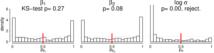
Figure 1: VSBC diagnostics for $\beta_{1},\beta_{2}$ and $\log\sigma$ in the Bayesian linear regression example. The VI estimation overestimates $\sigma$ as $p_{\sigma}$ is right-skewed, while $\beta_{1}$ and $\beta_{2}$ is unbiased as the two-sided KS-test is not rejected.

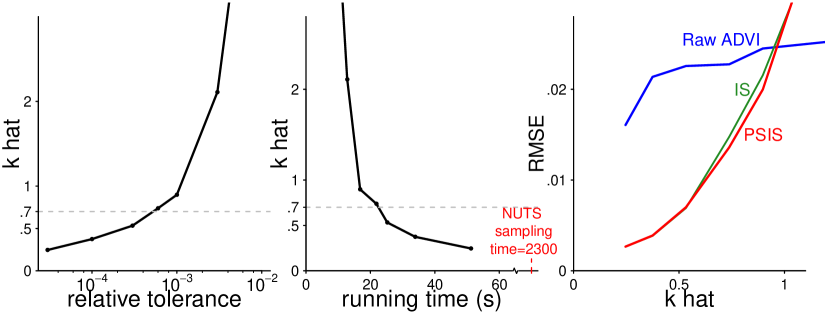
Figure 2: ADVI is sensitive to the stopping time in the linear regression example. The default 0.01 threshold lead to a fake convergence, which can be diagnosed by monitoring PSIS $\hat{k}$. PSIS adjustment always shrinks the estimation errors.

4.2 Logistic Regression

Next we run ADVI to a logistic regression $Y\sim\mathrm{Bernoulli}\left(\mathrm{logit}^{-1}(\beta X)\right)$ with a flat prior on $\beta$. We generate $X=(x_{1},\dots,x_{n})$ from $\hbox{N}(0,(1-\rho)I_{K\times K}+\rho 1_{K\times K})$ such that the correlation in design matrix is $\rho$, and $\rho$ is changed from 0 to 0.99. The first panel in Figure 3 shows PSIS $\hat{k}$ increases as the design matrix correlation increases. It is not monotonic because $\beta$ is initially negatively correlated when $X$ is independent. A large $\rho$ transforms into a large correlation for posterior distributions in $\beta$, making it harder to be approximated by a mean-field family, as can be diagnosed by $\hat{k}$. In panel 2 we calculate mean log predictive density (lpd) of VI approximation and true posterior using 200 independent test sets. Larger $\rho$ leads to worse mean-field approximation, while prediction becomes easier. Consequently, monitoring lpd does not diagnose the VI behavior; it increases (misleadingly suggesting better fit) as $\rho$ increases. In this special case, VI has larger lpd than the true posterior, due to the VI under-dispersion and the model misspecification. Indeed, if viewing lpd as a function $h(\beta)$, it is the discrepancy between VI lpd and true lpd that reveals the VI performance, which can also be diagnosed by $\hat{k}$. Panel 3 shows a sharp increase of lpd discrepancy around $\hat{k}=0.7$, consistent with the empirical threshold we suggest.

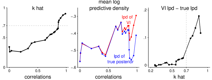
Figure 3: In the logistic regression example, as the correlation in design matrix increase, the correlation in parameter space also increases, leading to larger $\hat{k}$. Such flaw is hard to tell from the VI log predictive density (lpd), as a larger correlation makes the prediction easier. $\hat{k}$ diagnose the discrepancy of VI lpd and true posterior lpd, with a sharp jump at $0.7$.

Figure 4 compares the first and second moment root mean square errors (RMSE) $||E_{p}\beta-E_{q^{*}}\beta||_{2}$ and $||E_{p}\beta^{2}-E_{q^{*}}\beta^{2}||_{2}$ in the previous example using three estimates: (a) VI without post-adjustment, (b) VI adjusted by vanilla importance sampling, and (c) VI adjusted by PSIS.

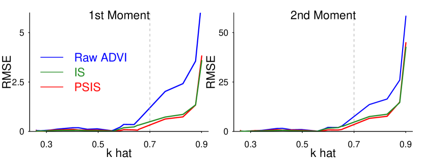
Figure 4: In the logistic regression with varying correlations, the $\hat{k}$ diagnoses the root mean square of first and second moment errors. No estimation is reliable when $\hat{k}>0.7$. Meanwhile, PSIS adjustment always shrinks the VI estimation errors.

PSIS diagnostic accomplishes two tasks here: (1) A small $\hat{k}$ indicates that VI approximation is reliable. When $\hat{k}>0.7$, all estimations are no longer reasonable so the user should be alerted. (2) It further improves the approximation using PSIS adjustment, leading to a quicker convergence rate and smaller mean square errors for both first and second moment estimation. Plain importance sampling has larger RMSE for it suffers from a larger variance.

4.3 Re-parametrization in a Hierarchical Model

The Eight-School Model (Gelman et al., 2013, Section 5.5) is the simplest Bayesian hierarchical normal model. Each school reported the treatment effect mean $y_{i}$ and standard deviation $\sigma_{i}$ separately. There was no prior reason to believe that any of the treatments were more effective than any other, so we model them as independent experiments:

$$y_{j}|\theta_{j} \sim\mbox{N}(\theta_{j},\sigma_{j}^{2}),\quad\theta_{j}|\mu,\tau\sim\mbox{N}(\mu,\tau^{2}),\quad 1\leq j\leq 8,$$

$$\mu \sim\operatorname{\mbox{N}}(0,5),\quad\quad\tau\sim\mathrm{half\!\!-\!\!Cauchy}(0,5).$$

where $\theta_{j}$ represents the treatment effect in school $j$, and $\mu$ and $\tau$ are the hyper-parameters shared across all schools.

In this hierarchical model, the conditional variance of $\theta$ is strongly dependent on the standard deviation $\tau$, as shown by the joint sample of $\mu$ and $\log\tau$ in the bottom-left corner in Figure 5. The Gaussian assumption in ADVI cannot capture such structure. More interestingly, ADVI over-estimates the posterior variance for all parameters $\theta_{1}$ through $\theta_{8}$, as shown by positive biases of their posterior standard deviation in the last panel. In fact, the posterior mode is at $\tau=0$, while the entropy penalization keeps VI estimation away from it, leading to an overestimation due to the funnel-shape. Since the conditional expectation $\operatorname{\mathrm{E}}[\theta_{i}|\tau,y,\sigma]=\left({\sigma_{j}^{-2}}+{\tau^{-2}}\right)^{-1}$ is an increasing function on $\tau$, a positive bias of $\tau$ produces over-dispersion of $\theta$.

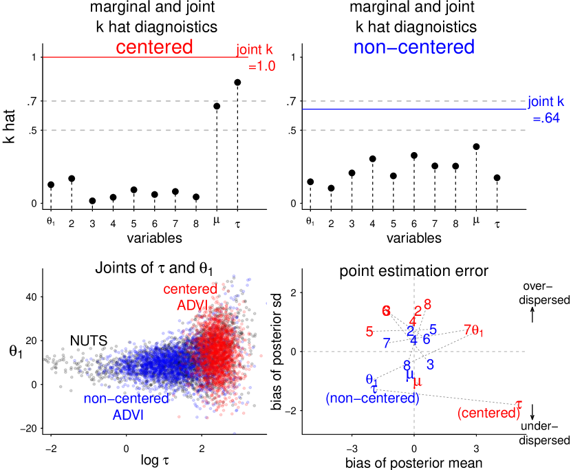
Figure 5: The upper two panels shows the joint and marginal PSIS diagnostics of the eight-school example. The centered parameterization has $\hat{k}>0.7$, for it cannot capture the funnel-shaped dependency between $\tau$ and $\theta$. The bottom-right panel shows the bias of posterior mean and standard errors of marginal distributions. Positive bias of $\tau$ leads to over-dispersion of $\theta$.

The top left panel shows the marginal and joint PSIS diagnostics. The joint $\hat{k}$ is 1.00, much beyond the threshold, while the marginal $\hat{k}$ calculated through the true marginal distribution for all $\theta$ are misleadingly small due to the over-dispersion.

Alerted by such large $\hat{k}$, researchers should seek some improvements, such as re-parametrization. The non-centered parametrization extracts the dependency between $\theta$ and $\tau$ through a transformation $\theta^{*}=(\theta-\mu)/\tau$:

$$y_{j}|\theta_{j}\sim\mbox{N}(\mu+\tau\theta^{*}_{j},\sigma_{j}^{2}),\quad\theta^{*}_{j}\sim\mbox{N}(0,1).$$

There is no general rule to determine whether non-centered parametrization is better than the centered one and there are many other parametrization forms. Finding the optimal parametrization can be as hard as finding the true posterior, but $\hat{k}$ diagnostics always guide the choice of parametrization. As shown by the top right panel in Figure 5, the joint $\hat{k}$ for the non-centered ADVI decreases to $0.64$ which indicated the approximation is not perfect but reasonable and usable. The bottom-right panel demonstrates that the re-parametrized ADVI posterior is much closer to the truth, and has smaller biases for both first and second moment estimations.

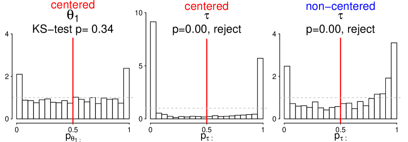
Figure 6: In the eight-school example, the VSBC diagnostic verifies VI estimation of $\theta_{1}$ is unbiased as the distribution of $p_{\theta_{1:}}$ is symmetric. $\tau$ is overestimated in the centered parametrization and underestimated in the non-centered one, as told by the right/ left skewness of $p_{\tau:}$.

We can assess the marginal estimation using VSBC diagnostic, as summarized in Figure 6. In the centered parametrization, the point estimation for $\theta_{1}$ is in average unbiased, as the two-sided KS-test is not rejected. The histogram for $\tau$ is right-skewed, for we can reject one-sided KS-test with the alternative to be $p_{\tau:}$ being stochastically smaller than $p_{\tau:}$. Hence we conclude $\tau$ is over-estimated in the centered parameterization. On the contrast, the non-centered $\tau$ is negatively biased, as diagnosed by the left-skewness of $p_{\tau:}$. Such conclusion is consistent with the bottom-right panel in Figure 5.

To sum up, this example illustrates how the Gaussian family assumption can be unrealistic even for a simple hierarchical model. It also clarifies VI posteriors can be both over-dispersed and under-dispersed, depending crucially on the true parameter dependencies. Nevertheless, the recommended PSIS and VSBC diagnostics provide a practical summary of the computation result.

4.4 Cancer Classification Using Horseshoe Priors

We illustrate how the proposed diagnostic methods work in the Leukemia microarray cancer dataset that contains $D=7129$ features and $n=72$ observations. Denote $y_{1:n}$ as binary outcome and $X_{n\times D}$ as the predictor, the logistic regression with a regularized horseshoe prior (Piironen & Vehtari, 2017) is given by

$$y|\beta\sim\mathrm{Bernoulli}\left(\mathrm{logit}^{-1}\left(X\beta\right)\right),\quad\beta_{j}|\tau,\lambda,c\sim\operatorname{\mbox{N}}(0,\tau^{2}\tilde{\lambda}_{j}^{2}),$$

$$\lambda_{j}\sim\mathrm{C}^{+}(0,1),\quad\tau\sim\mathrm{C}^{+}(0,\tau_{0}),\quad c^{2}\sim\mathrm{Inv\!\!-\!\!Gamma}(2,8).$$

where $\tau>0$ and $\lambda>0$ are global and local shrinkage parameters, and $\tilde{\lambda}_{j}^{2}=c^{2}\lambda_{j}^{2}/\left(c^{2}+\tau^{2}\lambda_{j}^{2}\right)$. The regularized horseshoe prior adapts to the sparsity and allows us to specify a minimum level of regularization to the largest values.

ADVI is computationally appealing for it only takes a few minutes while MCMC sampling takes hours on this dataset. However, PSIS diagnostic gives $\hat{k}=9.8$ for ADVI, suggesting the VI approximation is not even close to the true posterior. Figure 7 compares the ADVI and true posterior density of $\beta_{1834}$, $\log\lambda_{1834}$ and $\tau$. The Gaussian assumption makes it impossible to recover the bimodal distribution of some $\beta$.

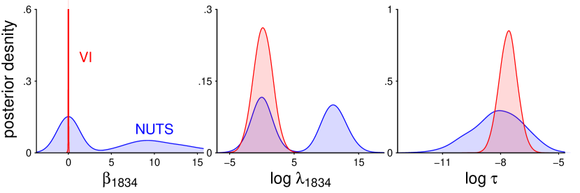
Figure 7: The comparison of ADVI and true posterior density of $\theta_{1834}$, $\log\lambda_{1834}$ and $\tau$ in the horseshoe logistic regression. ADVI misses the right mode of $\log\lambda$, making $\beta\propto\lambda$ become a spike.

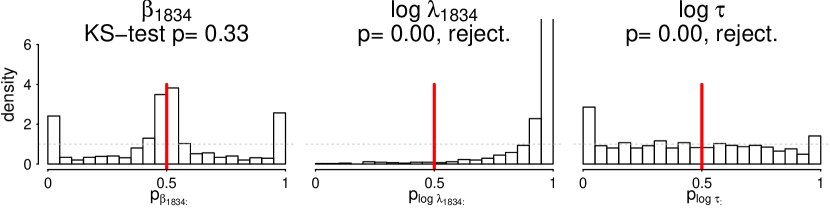
Figure 8: VSBC test in the horseshoe logistic regression. It tells the positive bias of $\tau$ and negative bias of $\lambda_{1834}$. $\beta_{1834}$ is in average unbiased for its symmetric prior.

The VSBC diagnostics as shown in Figure 8 tell the negative bias of local shrinkage $\lambda_{1834}$ from the left-skewness of $p_{\log\lambda_{1834}}$, which is the consequence of the right-missing mode. For compensation, the global shrinkage $\tau$ is over-estimated, which is in agreement with the right-skewness of $p_{\log\tau}$. $\beta_{1834}$ is in average unbiased, even though it is strongly underestimated from in Figure 7. This is because VI estimation is mostly a spike at 0 and its prior is symmetric. As we have explained, passing the VSBC test means the average unbiasedness, and does not ensure the unbiasedness for a specific parameter setting. This is the price that VSBC pays for averaging over all priors.

5 Discussion

5.1 The Proposed Diagnostics are Local

As no single diagnostic method can tell all problems, the proposed diagnostic methods have limitations. The PSIS diagnostic is limited when the posterior is multimodal as the samples drawn from $q(\theta)$ may not cover all the modes of the posterior and the estimation of $k$ will be indifferent to the unseen modes. In this sense, the PSIS diagnostic is a local diagnostic that will not detect unseen modes. For example, imagine the true posterior is $p=0.8\mbox{N}(0,0.2)+0.2\mbox{N}(3,0.2)$ with two isolated modes. Gaussian family VI will converge to one of the modes, with the importance ratio to be a constant number $0.8$ or $0.2$. Therefore ${k}$ is 0, failing to penalize the missing density. In fact, any divergence measure based on samples from the approximation such as $\operatorname{\mathrm{KL}}(q,p)$ is local.

The bi-modality can be detected by multiple over-dispersed initialization. It can also be diagnosed by other divergence measures such as $\operatorname{\mathrm{KL}}(p,q)=\operatorname{\mathrm{E}}_{p}\log(q/p)$, which is computable through PSIS by letting $h=\log(q/p)$.

In practice a marginal missing mode will typically lead to large joint discrepancy that is still detectable by $\hat{k}$, such as in Section 4.4.

The VSBC test, however, samples the true parameter from the prior distribution directly. Unless the prior is too restrictive, the VSBC $p$-value will diagnose the potential missing mode.

5.2 Tailoring Variational Inference for Importance Sampling

The PSIS diagnostic makes use of stabilized IS to diagnose VI. By contrast, can we modify VI to give a better IS proposal?

Geweke (1989) introduce an optimal proposal distribution based on split-normal and split-$t$, implicitly minimizing the $\chi^{2}$ divergence between $q$ and $p$. Following this idea, we could first find the usual VI solution, and then switch Gaussian to Student-$t$ with a scale chosen to minimize the $\chi^{2}$ divergence.

More recently, some progress is made to carry out variational inference based on Rényi divergence (Li & Turner, 2016; Dieng et al., 2017). But a big $\alpha$, say $\alpha=2$, is only meaningful when the proposal has a much heavier tail than the target. For example, a normal family does not contain any member having finite $\chi^{2}$ divergence to a Student-$t$ distribution, leaving the optimal objective function defined by Dieng et al. (2017) infinitely large.

There are several research directions. First, our proposed diagnostics are applicable to these modified approximation methods. Second, PSIS re-weighting will give a more reliable importance ratio estimation in the Rényi divergence variational inference. Third, a continuous $\hat{k}$ and the corresponding $\alpha$ are more desirable than only fixing $\alpha=2$, as the latter one does not necessarily have a finite result. Considering the role $\hat{k}$ plays in the importance sampling, we can optimize the discrepancy $D_{\alpha}(q||p)$ and $\alpha>0$ simultaneously. We leave this for future research.

Appendix A Sketch of Proofs

A.1 Proof to Proposition 1: Marginal $\hat{k}$ in PSIS diagnostic

Proposition 1.

For any two distributions $p$ and $q$ with support $\Theta$ and the margin index $i$, if there is a number $\alpha>1$ satisfying $E_{q}\left(p(\theta)/q(\theta)\right)^{\alpha}<\infty$, then $E_{q}\left(p(\theta_{i})/q(\theta_{i})\right)^{\alpha}<\infty$.

Proof.

Without loss of generality, we could assume $\Theta=\operatorname{\mathbb{R}}^{K}$, otherwise a smooth transformation is conducted.

For any $1\leq i\leq K$, $p(\theta_{-i}|\theta_{i})$ and $q(\theta_{-i}|\theta_{i})$ define the conditional distribution of $\left(\theta_{1},\dots,\theta_{i-1},\theta_{i+1},\dots,\theta_{K}\right)\in\operatorname{\mathbb{R}}^{K-1}$ given $\theta_{i}$ under the true posterior $p$ and the approximation $q$ separately.

For any given index $\alpha>1$, Jensen inequality yields

$$\int_{\operatorname{\mathbb{R}}^{K-1}}\left(\frac{p(\theta_{-i}|\theta_{i})}{q(\theta_{-i}|\theta_{i})}\right)^{\alpha}q(\theta_{-i}|\theta_{i})\geq\left(\int_{\operatorname{\mathbb{R}}^{K-1}}\frac{p(\theta_{-i}|\theta_{i})}{q(\theta_{-i}|\theta_{i})}q(\theta_{-i}|\theta_{i})\right)^{\alpha}=1$$

Hence

$$\int_{\operatorname{\mathbb{R}}^{K}}\left(\frac{p(\theta)}{q(\theta)}\right)^{\alpha}q(\theta)d\theta =\int_{\operatorname{\mathbb{R}}^{K-1}}\int_{\operatorname{\mathbb{R}}}\left(\frac{p(\theta_{i})p(\theta_{-i}|\theta_{i})}{q(\theta_{i})q(\theta_{-i}|\theta_{i})}\right)^{\alpha}q(\theta_{i})q(\theta_{-i}|\theta_{i})d\theta_{i}d\theta_{-i}$$

$$=\int_{\operatorname{\mathbb{R}}}\left(\int_{\operatorname{\mathbb{R}}^{K-1}}\left(\frac{p(\theta_{-i}|\theta_{i})}{q(\theta_{-i}|\theta_{i})}\right)^{\alpha}q(\theta_{-i}|\theta_{i})d\theta_{-i}\right)\left(\frac{p(\theta_{i})}{q(\theta_{i})}\right)^{\alpha}q(\theta_{i})d\theta_{i}$$

$$\geq\int_{\operatorname{\mathbb{R}}}\left(\frac{p(\theta_{i})}{q(\theta_{i})}\right)^{\alpha}q(\theta_{i})d\theta_{i}$$

∎

A.2 Proof to Proposition 2: Symmetry in VSBC-Test

Proposition 2.

For a one-dimensional parameter $\theta$ that is of interest, Suppose in addition we have:
(i) the VI approximation $q$ is symmetric;
(ii) the true posterior $p(\theta|y)$ is symmetric.
If the VI estimation $q$ is unbiased, i.e.,

$$\operatorname{\mathrm{E}}_{\theta\sim q(\theta|y)}\theta=\operatorname{\mathrm{E}}_{\theta\sim p(\theta|y)}\theta,\forall y$$

Then the distribution of VSBC $p$-value is symmetric.
If the VI estimation is positively/negatively biased, then the distribution of VSBC $p$-value is right/left skewed.

In the proposition we write $q(\theta|y)$ to emphasize that the VI approximation also depends on the observed data.

Proof.

First, as the same logic in (Cook et al., 2006), when $\theta^{(0)}$ is sampled from its prior $p(\theta)$ and simulated data $y$ sampled from likelihood $p(y|\theta^{(0)})$, $(y,\theta^{(0)})$ represents a sample from the joint distribution $p(y,\theta)$ and therefore $\theta^{(0)}$ can be viewed as a draw from $p(\theta|y)$, the true posterior distribution of $\theta$ with $y$ being observed.

We denote $q(\theta^{(0)})$ as the VSBC $p$-value of the sample $\theta^{(0)}$. Also denote $Q_{x}(f)$ as the $x-$quantile ($x\in[0,1]$) of any distribution $f$. To prove the result, we need to show

$$1-\Pr(q(\theta^{(0)})<x)=\Pr(q(\theta^{(0)})<1-x),\forall x\in[0,1],$$

$$\mathrm{LHS} =\Pr\left(q(\theta^{(0)})>x\right)$$

$$=\Pr\left(\theta^{(0)}>Q_{x}\left(q(\theta|y)\right)\right).$$

$$\mathrm{RHS}=\Pr\left(\theta^{(0)}<Q_{1-x}\left(q(\theta|y)\right)\right) =\Pr\left(\theta^{(0)}<2E_{q(\theta|y)}\theta-Q_{x}\left(q(\theta|y)\right)\right)$$

$$=\Pr\left(\theta^{(0)}<2E_{p(\theta|y)}\theta-Q_{x}\left(q(\theta|y)\right)\right)$$

$$=\Pr\left(\theta^{(0)}>Q_{x}\left(q(\theta|y)\right)\right)$$

$$=\mathrm{LHS}$$

The first equation above uses the symmetry of $q(\theta|y)$, the second equation comes from the the unbiasedness condition. The third is the result of the symmetry of $p(\theta|y)$.

If the VI estimation is positively biased, $\operatorname{\mathrm{E}}_{\theta\sim q(\theta|y)}\theta>\operatorname{\mathrm{E}}_{\theta\sim p(\theta|y)}\theta,\forall y,$ then we change the second equality sign into a less-than sign. ∎

Appendix B Details of Simulation Examples

In this section, we give more detailed description of the simulation examples in the manuscript. We use Stan (Stan Development Team, 2017) to implement both automatic differentiation variational inference (ADVI) and Markov chain Monte Carlo (MCMC) sampling. We implement Pareto smoothing through R package “loo” (Vehtari et al., 2018). We also provide all the source code in https://github.com/yao-yl/Evaluating-Variational-Inference.

B.1 Linear and Logistic Regressions

In Section 4.1, We start with a Bayesian linear regression $y\sim\operatorname{\mbox{N}}(X\beta,\sigma^{2})$ without intercept. The prior is set as $\{\beta_{i}\}_{i=1}^{d}\sim\operatorname{\mbox{N}}(0,1),\sigma\sim\mathrm{gamma}(0.5,0.5)$. We fix sample size $n=10000$ and number of regressors $d=100$. Figure IX displays the Stan code.

⬇

,

1 data {

2 int <lower=0> n; //number of observations, we fix n=10000 in the simulation;

3 int <lower=0> d; //number of predictor variables, fix d=100;

4 matrix [n,d] x ; // predictors;

5 vector [n] y; // outcome;

6 }

7 parameters {

8 vector [d] b; // linear regression coefficient;

9 real <lower=0> sigma; //linear regression std;

10 }

11 model {

12 y $\sim$ normal(x * b, sigma);

13 b $\sim$ normal(0,1); // prior for regression coefficient;

14 sigma $\sim$ gamma(0.5,0.5); // prior for regression std.

15 }

Figure IX: Stan code for linear regressions

We find ADVI can be sensitive to the stopping time. Part of the reason is the objective function itself is evaluated through Monte Carlo samples, producing large uncertainty. In the current version of Stan, ADVI computes the running average and running median of the relative ELBO norm changes. Should either number fall below a threshold tol_rel_obj, with the default value to be 0.01, the algorithm is considered converged.

In Figure 1 of the main paper, we run VSBC test on ADVI approximation. ADVI is deliberately tuned in a conservative way. The convergence tolerance is set as tol_rel_obj=$10^{-4}$ and the learning rate is $\eta=0.05$. The predictor $X_{10^{5}\times 10^{2}}$ is fixed in all replications and is generated independently from $\operatorname{\mbox{N}}(0,1)$. To avoid multiple-comparison problem, we pre-register the first and second coefficients $\beta_{1}$ $\beta_{2}$ and $\log\sigma$ before the test. The VSBC diagnostic is based on $M=1000$ replications.

In Figure 2 we independently generate each coordinate of $\beta$ from $\operatorname{\mbox{N}}(0,1)$ and set a relatively large variance $\sigma=2$. The predictor $X$ is generated independently from $\operatorname{\mbox{N}}(0,1)$ and $y$ is sampled from the normal likelihood. We vary the threshold tol_rel_obj from $0.01$ to $10^{-5}$ and show the trajectory of $\hat{k}$ diagnostics. The $\hat{k}$ estimation, IS and PSIS adjustment are all calculated from $S=5\times 10^{4}$ posterior samples. We ignore the ADVI posterior sampling time. The actual running time is based on a laptop experiment result (2.5 GHz processor, 8 cores).The exact sampling time is based on the No-U-Turn Sampler (NUTS, Hoffman & Gelman 2014) in Stan with 4 chains and 3000 iterations in each chain. We also calculate the root mean square errors (RMSE) of all parameters $||E_{p}[(\beta,\sigma)]-E_{q}[(\beta,\sigma)]||_{L^{2}}$, where $(\beta,\sigma)$ represents the combined vector of all $\beta$ and $\sigma$. To account for the uncertainty, $\hat{k}$, running time, and RMSE takes the average of 50 repeated simulations.

⬇

,

1 data {

2 int <lower=0> n; //number of observations;

3 int <lower=0> d; //number of predictor variables;

4 matrix [n,d] x ; // predictors; we vary its correlation during simulations.

5 int<lower=0,upper=1> y[n]; // binary outcome;

6 }

7 parameters {

8 vector[d] beta;

9 }

10 model {

11 y $\sim$ bernoulli_logit(x*beta);

12 }

Figure X: Stan code for logistic regressions

Figure 3 and 4 in the main paper is a simulation result of a logistic regression

$$Y\sim\mathrm{Bernoulli}\left(\mathrm{logit}^{-1}(\beta X)\right)$$

with a flat prior on $\beta$. We vary the correlation in design matrix by generating $X$ from $\hbox{N}(0,(1-\rho)I_{d\times d}+\rho 1_{d\times d})$, where $1_{d\times d}$ represents the $d$ by $d$ matrix with all elements to be $1$. In this experiment we fix a small number $n=100$ and $d=2$ since the main focus is parameter correlations. We compare $\hat{k}$ with the log predictive density, which is calculated from 100 independent test data. The true posterior is from NUTS in Stan with 4 chains and 3000 iterations each chain. The $\hat{k}$ estimation, IS and PSIS adjustment are calculated from $10^{5}$ posterior samples. To account for the uncertainty, $\hat{k}$, log predictive density, and RMSE are the average of 50 repeated experiments.

B.2 Eight-School Model

The eight-school model is named after Gelman et al. (2013, section 5.5). The study was performed for the Educational Testing Service to analyze the effects of a special coaching program on students’ SAT-V (Scholastic Aptitude Test Verbal) scores in each of eight high schools. The outcome variable in each study was the score of a standardized multiple choice test. Each school $i$ separately analyzed the treatment effect and reported the mean $y_{i}$ and standard deviation of the treatment effect estimation $\sigma_{i}$, as summarized in Table 1.

School Index $j$	Estimated Treatment Effect $y_{i}$	Standard Deviation of Effect Estimate $\sigma_{j}$
1	28	15
2	8	10
3	-3	16
4	7	11
5	-1	9
6	1	11
7	8	10
8	12	18

Table 1: School-level observed effects of special preparation on SAT-V scores in eight randomized experiments. Estimates are based on separate analyses for the eight experiments.

There was no prior reason to believe that any of the eight programs was more effective than any other or that some were more similar in effect to each other than to any other. Hence, we view them as independent experiments and apply a Bayesian hierarchical normal model:

$$y_{j}|\theta_{j} \sim\mbox{N}(\theta_{j},\sigma_{j}),\quad\theta_{j}\sim\mbox{N}(\mu,\tau),\quad 1\leq j\leq 8,$$

$$\mu \sim\operatorname{\mbox{N}}(0,5),\quad\quad\tau\sim\mathrm{half\!\!-\!\!Cauchy}(0,5).$$

where $\theta_{j}$ represents the underlying treatment effect in school $j$, while $\mu$ and $\tau$ are the hyper-parameters that are shared across all schools.

⬇

,

1 data {

2 int<lower=0> J; // number of schools

3 real y[J]; // estimated treatment

4 real<lower=0> sigma[J]; // std of estimated effect

5 }

6

7 parameters {

8 real theta[J]; // treatment effect in school j

9 real mu; // hyper-parameter of mean

10 real<lower=0> tau; // hyper-parameter of sdv

11 }

12 model {

13 theta $\sim$ normal(mu, tau);

14 y $\sim$ normal(theta, sigma);

15 mu $\sim$ normal(0, 5); // a non-informative prior

16 tau $\sim$ cauchy(0, 5);

17 }

Figure XI: Stan code for centered parametrization in the eight-school model. It leads to strong dependency between $tau$ and $theta$.

⬇

,

1 data {

2 int<lower=0> J; // number of schools

3 real y[J]; // estimated treatment

4 real<lower=0> sigma[J]; // std of estimated effect

5 }

6 parameters {

7 vector[J] theta_trans; // transformation of theta

8 real mu; // hyper-parameter of mean

9 real<lower=0> tau; // hyper-parameter of sd

10 }

11 transformed parameters{

12 vector[J] theta; // original theta

13 theta=theta_trans*tau+mu;

14 }

15 model {

16 theta_trans $\sim$normal (0,1);

17 y $\sim$ normal(theta, sigma);

18 mu $\sim$ normal(0, 5); // a non-informative prior

19 tau $\sim$ cauchy(0, 5);

20 }

Figure XII: Stan code for non-centered parametrization in the eight-school model. It extracts the dependency between $tau$ and $theta$.

There are two parametrization forms being discussed: centered parameterization and non-centered parameterization. Listing XI and XII give two Stan codes separately. The true posterior is from NUTS in Stan with 4 chains and 3000 iterations each chain. The $\hat{k}$ estimation and PSIS adjustment are calculated from $S=10^{5}$ posterior samples. The marginal $\hat{k}$ is calculated by using the NUTS density, which is typically unavailable for more complicated problems in practice.

The VSBC test in Figure 6 is based on $M=1000$ replications and we pre-register the first treatment effect $\theta_{1}$ and group-level standard error $\log\tau$ before the test.

As discussed in Section 3.2, VSBC assesses the average calibration of the point estimation. Hence the result depends on the choice of prior. For example, if we instead set the prior to be

$$\mu\sim\operatorname{\mbox{N}}(0,50),\quad\quad\tau\sim\mathrm{N}^{+}(0,25),$$

which is essentially flat in the region of interesting part of the likelihood and more in agreement with the prior knowledge, then the result of VSBC test change to Figure XIII. Again, the skewness of $p$-values verifies VI estimation of $\theta_{1}$ is in average unbiased while $\tau$ is biased in both centered and non-centered parametrization.

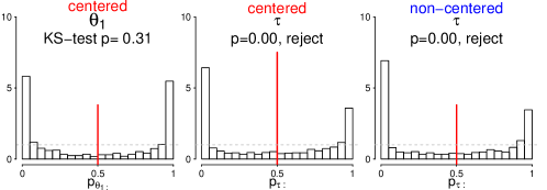
Figure XIII: The VSBC diagnostic of the eight-school example under a non-informative prior $\mu\sim\operatorname{\mbox{N}}(0,50),\,\tau\sim\mathrm{N}^{+}(0,25)$. The skewness of $p$-values verifies VI estimation of $\theta_{1}$ is in average unbiased while $\tau$ is biased in both centered and non-centered parametrization.

B.3 Cancer Classification Using Horseshoe Priors

In Section 4.3 of the main paper we replicate the cancer classification under regularized horseshoe prior as first introduced by Piironen & Vehtari (2017).

The Leukemia microarray cancer classification dataset . It contains $n=72$ observations and $d=7129$ features $X_{n\times d}$. $X$ is standardized before any further process. The outcome $y_{1:n}$ is binary, so we can fit a logistic regression

$$y_{i}|\beta\sim\mathrm{Bernoulli}\left(\mathrm{logit}^{-1}\left(\sum_{j=1}^{d}\beta_{j}x_{ij}+\beta_{0}\right)\right).$$

There are far more predictors than observations, so we expect only a few of predictors to be related and therefore have a regression coefficient distinguishable from zero. Further, many predictors are correlated, making it necessary to have a regularization.

To this end, we apply the regularized horseshoe prior, which is a generalization of horseshoe prior.

$$\beta_{j}|\tau,\lambda,c\sim\operatorname{\mbox{N}}(0,\tau^{2}\tilde{\lambda}_{j}^{2}),\quad\quad c^{2}\sim\mathrm{Inv\!\!-\!\!Gamma}(2,8),$$

$$\lambda_{j}\sim\mathrm{Half\!\!-\!\!Cauchy}(0,1),\quad\tau|\tau_{0}\sim\mathrm{Half\!\!-\!\!Cauchy}(0,\tau_{0}).$$

The scale of the global shrinkage is set according to the recommendation $\tau_{0}=2\left(n^{1/2}(d-1)\right)^{-1}$ There is no reason to shrink intercept so we put $\beta_{0}\sim\operatorname{\mbox{N}}(0,10)$. The Stan code is summarized in Figure LABEL:ls_HS.

We first run NUTS in Stan with 4 chains and 3000 iterations each chain. We manually pick $\beta_{1834}$, the coefficient that has the largest posterior mean. The posterior distribution of it is bi-modal with one spike at 0.

ADVI is implemented using the same parametrization and we decrease the learning rate $\eta$ to 0.1 and the threshold tol_rel_obj to $0.001$

The $\hat{k}$ estimation is based on $S=10^{4}$ posterior samples. Since $\hat{k}$ is extremely large, indicating VI is far away from the true posterior and no adjustment will work, we do not further conduct PSIS.

⬇

,

1 data {

2 int<lower=0> n; // number of observations

3 int<lower=0> d; // number of predictors

4 int<lower=0,upper=1> y[n]; // outputs

5 matrix[n,d] x; // inputs

6 real<lower=0> scale_icept; // prior std for the intercept

7 real<lower=0> scale_global; // scale for the half-t prior for tau

8 real<lower=0> slab_scale;

9 real<lower=0> slab_df;

10 }

11 parameters {

12 real beta0; // intercept

13 vector[d] z; // auxiliary parameter

14 real<lower=0> tau; // global shrinkage parameter

15 vector<lower=0>[d] lambda; // local shrinkage parameter

16 real<lower=0> caux; // auxiliary

17 }

18 transformed parameters {

19 real<lower=0> c;

20 vector[d] beta; // regression coefficients

21 vector[n] f; // latent values

22 vector<lower=0>[d] lambda_tilde;

23 c = slab_scale * sqrt(caux);

24 lambda_tilde = sqrt( c^2 * square(lambda) ./ (c^2 + tau^2* square(lambda)) );

25 beta = z .* lambda_tilde*tau;

26 f = beta0 + x*beta;

27 }

28 model {

29 z $\sim$ normal(0,1);

30 lambda $\sim$ cauchy(0,1);

31 tau $\sim$ cauchy(0, scale_global);

32 caux $\sim$ inv_gamma(0.5*slab_df, 0.5*slab_df);

33 beta0 $\sim$ normal(0,scale_icept);

34 y $\sim$ bernoulli_logit(f);

35 } \end{lstlisting}\caption{\em Stan code for regularized horseshoe logistic regression.}\label{ls_HS}

36\end{figure}

37

38

39In the VSBC test, we pre-register that pre-chosen coefficient $\beta_{1834}$, $\log \lambda_{1834}$ and global shrinkage $\log \tau$ before the test. The VSBC diagnostic is based on M=1000 replications.

References

- Anderson (1996) Anderson, J. L. A method for producing and evaluating probabilistic forecasts from ensemble model integrations. Journal of Climate, 9(7):1518–1530, 1996.
- Blei et al. (2017) Blei, D. M., Kucukelbir, A., and McAuliffe, J. D. Variational inference: A review for statisticians. Journal of the American Statistical Association, 112(518):859–877, 2017.
- Chee & Toulis (2017) Chee, J. and Toulis, P. Convergence diagnostics for stochastic gradient descent with constant step size. arXiv preprint arXiv:1710.06382, 2017.
- Chen et al. (2004) Chen, L. H., Shao, Q.-M., et al. Normal approximation under local dependence. The Annals of Probability, 32(3):1985–2028, 2004.
- Cook et al. (2006) Cook, S. R., Gelman, A., and Rubin, D. B. Validation of software for Bayesian models using posterior quantiles. Journal of Computational and Graphical Statistics, 15(3):675–692, 2006.
- Cortes et al. (2010) Cortes, C., Mansour, Y., and Mohri, M. Learning bounds for importance weighting. In Advances in neural information processing systems, pp. 442–450, 2010.
- Cortes et al. (2013) Cortes, C., Greenberg, S., and Mohri, M. Relative deviation learning bounds and generalization with unbounded loss functions. arXiv preprint arXiv:1310.5796, 2013.
- Dieng et al. (2017) Dieng, A. B., Tran, D., Ranganath, R., Paisley, J., and Blei, D. Variational inference via upper bound minimization. In Advances in Neural Information Processing Systems, pp. 2729–2738, 2017.
- Epifani et al. (2008) Epifani, I., MacEachern, S. N., Peruggia, M., et al. Case-deletion importance sampling estimators: Central limit theorems and related results. Electronic Journal of Statistics, 2:774–806, 2008.
- Gelman et al. (2013) Gelman, A., Carlin, J. B., Stern, H. S., Dunson, D. B., Vehtari, A., and Rubin, D. B. Bayesian data analysis. CRC press, 2013.
- Geweke (1989) Geweke, J. Bayesian inference in econometric models using Monte Carlo integration. Econometrica, 57(6):1317–1339, 1989.
- Giordano et al. (2017) Giordano, R., Broderick, T., and Jordan, M. I. Covariances, robustness, and variational Bayes. arXiv preprint arXiv:1709.02536, 2017.
- Hoffman & Gelman (2014) Hoffman, M. D. and Gelman, A. The No-U-Turn sampler: adaptively setting path lengths in Hamiltonian Monte Carlo. Journal of Machine Learning Research, 15(1):1593–1623, 2014.
- Hoffman et al. (2013) Hoffman, M. D., Blei, D. M., Wang, C., and Paisley, J. Stochastic variational inference. The Journal of Machine Learning Research, 14(1):1303–1347, 2013.
- Ionides (2008) Ionides, E. L. Truncated importance sampling. Journal of Computational and Graphical Statistics, 17(2):295–311, 2008.
- Koopman et al. (2009) Koopman, S. J., Shephard, N., and Creal, D. Testing the assumptions behind importance sampling. Journal of Econometrics, 149(1):2–11, 2009.
- Kucukelbir et al. (2017) Kucukelbir, A., Tran, D., Ranganath, R., Gelman, A., and Blei, D. M. Automatic differentiation variational inference. Journal of Machine Learning Research, 18(14):1–45, 2017.
- Li & Turner (2016) Li, Y. and Turner, R. E. Rényi divergence variational inference. In Advances in Neural Information Processing Systems, pp. 1073–1081, 2016.
- Pflug (1990) Pflug, G. C. Non-asymptotic confidence bounds for stochastic approximation algorithms with constant step size. Monatshefte für Mathematik, 110(3):297–314, 1990.
- Piironen & Vehtari (2017) Piironen, J. and Vehtari, A. Sparsity information and regularization in the horseshoe and other shrinkage priors. Electronic Journal of Statistics, 11(2):5018–5051, 2017.
- Ranganath et al. (2014) Ranganath, R., Gerrish, S., and Blei, D. Black box variational inference. In Artificial Intelligence and Statistics, pp. 814–822, 2014.
- Rényi et al. (1961) Rényi, A. et al. On measures of entropy and information. In Proceedings of the Fourth Berkeley Symposium on Mathematical Statistics and Probability, Volume 1: Contributions to the Theory of Statistics. The Regents of the University of California, 1961.
- Rezende et al. (2014) Rezende, D. J., Mohamed, S., and Wierstra, D. Stochastic backpropagation and approximate inference in deep generative models. In Proceedings of the 31st International Conference on Machine Learning (ICML-14), pp. 1278–1286, 2014.
- Sielken (1973) Sielken, R. L. Stopping times for stochastic approximation procedures. Probability Theory and Related Fields, 26(1):67–75, 1973.
- Stan Development Team (2017) Stan Development Team. Stan modeling language users guide and reference manual. http://mc-stan.org, 2017. Version 2.17.
- Stroup & Braun (1982) Stroup, D. F. and Braun, H. I. On a new stopping rule for stochastic approximation. Probability Theory and Related Fields, 60(4):535–554, 1982.
- Vehtari et al. (2017) Vehtari, A., Gelman, A., and Gabry, J. Pareto smoothed importance sampling. arXiv preprint arXiv:1507.02646, 2017.
- Vehtari et al. (2018) Vehtari, A., Gabry, J., Yao, Y., and Gelman, A. loo: Efficient leave-one-out cross-validation and waic for bayesian models, 2018. URL https://CRAN.R-project.org/package=loo. R package version 2.0.0.
- Wada & Fujisaki (2015) Wada, T. and Fujisaki, Y. A stopping rule for stochastic approximation. Automatica, 60:1–6, 2015. ISSN 0005-1098.