Directly and Efficiently Optimizing Prediction Error
and AUC of Linear Classifiers

Abstract

The predictive quality of machine learning models is typically measured in terms of their (approximate) expected prediction error or the so-called Area Under the Curve (AUC) for a particular data distribution. However, when the models are constructed by the means of empirical risk minimization, surrogate functions such as the logistic loss are optimized instead. This is done because the empirical approximations of the expected error and AUC functions are nonconvex and nonsmooth, and more importantly have zero derivative almost everywhere. In this work, we show that in the case of linear predictors, and under the assumption that the data has normal distribution, the expected error and the expected AUC are not only smooth, but have closed form expressions, which depend on the first and second moments of the normal distribution. Hence, we derive derivatives of these two functions and use these derivatives in an optimization algorithm to directly optimize the expected error and the AUC. In the case of real data sets, the derivatives can be approximated using empirical moments. We show that even when data is not normally distributed, computed derivatives are sufficiently useful to render an efficient optimization method and high quality solutions. Thus, we propose a gradient-based optimization method for direct optimization of the prediction error and AUC. Moreover, the per-iteration complexity of the proposed algorithm has no dependence on the size of the data set, unlike those for optimizing logistic regression and all other well known empirical risk minimization problems.

1 Introduction

In this paper, we consider classical binary linear classification problems in supervised Machine Learning (ML). In other words, given a finite set labeled data (labeled to form a positive and a negative class), the aim is to obtain a linear classifier that predicts the positive/negative labels of unseen data points as accurately as possible. To measure the accuracy of a classifier, the expected prediction error, which measures the percentage of mislabeled data points, also known as the $0-1$ loss function, is often used. However, since the empirical approximation of the prediction error is a nonsmooth nonconvex function, whose gradient is either zero or not defined. Hence, other surrogate loss functions are typically used to determine the linear classifier. For example, standard ML tools, such as support vector machines (Cortes & Vapnik, 1995; Osuna et al., 1997; Scholkopf et al., 1998) and logistic regression (Hosmer & Lemeshow, 2000), aim to optimize empirical prediction error, while using hinge loss and logistic loss, respectively, as surrogate functions of the $0-1$ loss function.

Many real world ML problems are dealing with imbalanced data sets, which contain rare positive data points, as the minority class, but numerous negative ones, as the majority class. When these two data classes are highly imbalanced, the prediction error function is not a useful prediction measure. For example, if the data set contains only $0.01\%$ of the positive examples, then a predictor that simply classifies every data point as negative has $99.99\%$ accuracy, while obviously failing to achieve any meaningful prediction. The prediction measure is often modified to incorporate class importance weights, in which case it can be used for imbalanced data sets. All results of this paper easily extend to such modification. However, a more established and robust measure of prediction accuracy which is used in practice is Area Under Receiver Operating Characteristic (ROC) Curve (AUC) (Hanley & McNeil, 1982). AUC is a reciprocal of the ranking loss, which is similar to the $0-1$ loss, in the sense that it measures the percentage of pairs of data samples, one from the negative class and one from the positive class, such that the classifier assigns a larger label to the negative sample than to the positive one. In other words, $1-$AUC counts the percentage of incorrectly “ranked” pairs (Mann & R.Whitney, 1947). The empirical approximation of AUC, just as that of $0-1$ loss, is a discontinuous, nonsmooth function, whose gradient is either zero or undefined. This difficulty motivates various techniques for optimizing continuous approximations of AUC. For example, the ranking loss can be replaced by convex loss functions such as pairwise logistic loss or hinge loss (Joachims, 2006; Steck, 2007; Rudin & Schapire, 2009; Zhao et al., 2011), which results in continuous convex optimization problem. A drawback of such approach, aside from the fact that a different objective is optimized, is that such loss has to be computed for each pair of data points, which significantly increases the complexity of the underlying optimization algorithm.

In this paper, we propose a novel method of directly optimizing the expected prediction error and the expected AUC value of a linear classifier in the case of binary classification problems. First, we use the probabilistic interpretation of the expected prediction error and we show that if the distribution of the positive and negative classes obey normal distributions, then the expected prediction error of a linear classifier is a smooth function with a closed-form expression. Thus, its gradient can be computed and a gradient-based optimization algorithm can be used. The closed form of the function depends on the first and second moments of the related normal distributions, hence these moments are needed to compute the function value as well as the gradient.

Similarly, under the assumption that the class of the positive and negative data sets jointly obey a normal distribution, we show that the corresponding expected AUC value of a linear classifier is a smooth function with closed form expression, which depends on the first and second moments of the distribution. Similarly to optimizing the prediction error, this novel result allows any gradient-based optimization algorithm to be applied to optimize the AUC value of a linear classifier.

Through empirical experiments we show that even when the data sets do not obey normal distribution, optimizing the derived functional forms of prediction error and AUC, using empirical approximate moments, often produces better predictors than those obtained by optimizing surrogate approximations, such as logistic and hinge losses. This behavior is in contrast with, for example, Linear Discriminant Analysis (LDA) (Izenman, 2013), which is the method to compute linear classifiers under the Gaussian assumption.

Another key advantage of the proposed method over the classical empirical risk minimization is that the training data is only used once at the beginning of the algorithm to compute the approximate moments. After that each iteration of an optimization algorithm only depends on the dimension of the classifier, while optimizing logistic loss or pairwise hinge loss using gradient-based method depends on the data size at each iteration.

The paper is organized as follows. In the next section we state preliminaries and the problem description. In Section 3 we show that the prediction error and AUC are smooth functions if the data obey normal distribution. We present computational results in Section 4, and finally, we state our conclusions in Section 5.

2 Preliminaries and Problem Description

We consider the classical setting of supervised machine learning, where we are given a finite training set $\mathcal{S}$ of $n$ pairs,

$$\mathcal{S}:=\{(x_{i},y_{i})~{}:~{}i=1,\cdots,n\},$$

where $x_{i}\in\mathbb{R}^{d}$ are the input vectors of features and $y_{i}\in\{+1,-1\}$ are the binary output labels. It is assumed that each pair $(x_{i},y_{i})$ is an i.i.d. sample of the random variable $(X,Y)$ with some unknown joint probability distribution $P_{X,Y}(x,y)$ over the input space $\mathcal{X}$ and output space $\mathcal{Y}$. The set $\mathcal{S}$ is known as a training set. The goal is to compute a linear classifier function $f:\mathcal{X}\to\mathcal{Y}$, so that given a random input variable $X$, $f$ can accurately predict the corresponding label $Y$.

As discussed in §1, there are two different performance measures to evaluate the quality of $f$: the prediction error, which approximates the expected risk, and the AUC. Expected risk of a linear classifier $f(x;w)=w^{T}x$ for 0-1 loss function is defined as

$$F_{error}\left(w\right) =\mathbb{E}_{\mathcal{X},\mathcal{Y}}\left[\ell_{01}\left(f(X;w),Y\right)\right]$$ (1)

$$=\int_{\mathcal{X}}\int_{\mathcal{Y}}P_{X,Y}(x,y)\ell_{01}\left(f(x;w),y\right)dydx,$$

where

$$\ell_{01}\left(f(x;w),y\right)=\begin{cases}+1&\text{if}~{}~{}y\cdot f(x;w)<0,\\ 0&\text{if}~{}~{}y\cdot f(x;w)\geq 0.\end{cases}$$

A finite sample approximation of (1), given a training set $\mathcal{S}$, is the following empirical risk

$$\hat{F}_{error}\left(w;\mathcal{S}\right)=\frac{1}{n}\sum_{i=1}^{n}\ell_{01}\left(f(x_{i};w),y_{i}\right).$$ (2)

The difficulty of optimizing (2), even approximately, arises from the fact that its gradient is either not defined or is equal to zero. Thus, gradient-based optimization methods cannot be applied. The most common alternative is to utilize the logistic regression loss function, as an approximation of the prediction error and solve the following unconstrained convex optimization problem

$$\min_{w\in\mathbb{R}^{d}}\hat{F}_{log}(w)= \frac{1}{n}\sum_{i=1}^{n}\log\left(1+\exp(-y_{i}\cdot f(x_{i};w))\right)$$ (3)

$$+\lambda r(w),$$

where $\lambda r(w)$ is the regularization term, with $r(\cdot)=\|\cdot\|_{1}$ or $r(\cdot)=\|\cdot\|_{2}$ as possible examples.

We now discuss the AUC function as the quality measure of a classifier, which is often the industry standard. For that let us define

$$\mathcal{S}^{+} :=\{x:(x,y)\in\mathcal{S},~{}y=+1\}$$

$$:=\{x_{i}^{+}~{}:~{}i=1,\cdots,n^{+}\},~{}~{}\text{where}~{}~{}x^{+}_{i}\in\mathbb{R}^{d}~{}~{}\text{and}$$

$$\mathcal{S}^{-} :=\{x:(x,y)\in\mathcal{S},~{}y=-1\}$$

$$:=\{x_{j}^{-}~{}:~{}j=1,\cdots,n^{-}\},~{}~{}\text{where}~{}~{}x^{-}_{j}\in\mathbb{R}^{d}.$$

Hence $\mathcal{S}^{+}$ and $\mathcal{S}^{-}$ are the sets of all positive and negative samples in $\mathcal{S}$, respectively, and they contain only inputs $x$, instead of pairs $(x,y)$. Let $|\mathcal{S}^{+}|=n^{+}$ and $|\mathcal{S}^{-}|=n^{-}$. The AUC value of a classifier $f(x;w)$, given the positive set $\mathcal{S}^{+}$ and the negative set $\mathcal{S}^{-}$ can be obtained via Wilcoxon-Mann-Whitney (WMW) statistic result (Mann & R.Whitney, 1947), e.g.,

$$\hat{F}_{AUC}\left(w;\mathcal{S}^{+},\mathcal{S}^{-}\right)$$ (4)

$$=\frac{\sum_{i=1}^{n^{+}}\sum_{j=1}^{n^{-}}\mathbbm{1}\left[f(x^{+}_{i};w)>f(x^{-}_{j};w)\right]}{n^{+}\cdot n^{-}},$$

where

$$\mathbbm{1}\left[f(x_{i}^{+};w)>f(x_{j}^{-};w)\right]$$

$$=\begin{cases}+1&\text{if}~{}~{}f(x_{i}^{+};w)>f(x_{j}^{-};w),\\ 0&\text{otherwise.}\end{cases}$$

Now, let $\mathcal{X}^{+}$ and $\mathcal{X}^{-}$ denote the space of the positive and negative input vectors, respectively, so that $x_{i}^{+}$ is an i.i.d. observation of the random variable $X^{+}$ from $\mathcal{X}^{+}$ and $x_{j}^{-}$ is an i.i.d. observation of the random variable $X^{-}$ from $\mathcal{X}^{-}$. Then, given the joint probability distribution $P_{X^{+},X^{-}}\left(x^{+},x^{-}\right)$, the expected AUC function of a classifier $f(x;w)$ is defined as

$$F_{AUC}(w)={} \mathbb{E}_{\mathcal{X}^{+},\mathcal{X}^{-}}\left[\mathbbm{1}\left[f\left(X^{+};w\right)>f\left(X^{-};w\right)\right]\right]$$ (5)

$$={} \int_{\mathcal{X}^{+}}\int_{\mathcal{X}^{-}}P_{X^{+},X^{-}}\left(x^{+},x^{-}\right)$$

$$\cdot\mathbbm{1}\left[f\left(x^{+};w\right)>f\left(x^{-};w\right)\right]dx^{-}dx^{+}.$$

The $\hat{F}_{AUC}\left(w;\mathcal{S}^{+},\mathcal{S}^{-}\right)$ computed by (4) is an unbiased estimator of $F_{AUC}(w)$. Similarly to the empirical risk minimization, the problem of optimizing AUC value of a predictor is not straightforward since the gradient of this function is either zero or not defined. Thus, gradient-based optimization methods cannot be applied.

As in the case of prediction error, various techniques have been proposed to approximate the AUC with a surrogate function. In (Yan et al., 2003), the indicator function $\mathbbm{1}[\cdot]$ in (4) is substituted with a sigmoid surrogate function, e.g., $1/\left({1+e^{-\beta\left(f(x^{+};w)-f(x^{-};w)\right)}}\right)$ and a gradient descent algorithm is applied to this smooth approximation. The choice of the parameter $\beta$ in the sigmoid function definition significantly affects the output of this approach; although a large value of $\beta$ renders a closer approximation of the step function, it also results in large oscillations of the gradients, which in turn can cause numerical issues in the gradient descent algorithm. Similarly, as is discussed in (Rudin & Schapire, 2009), pairwise exponential loss and pairwise logistic loss can be utilized as convex smooth surrogate functions of the indicator function $\mathbbm{1}[\cdot]$. In these settings, any gradient-based optimization method can be used to optimize the resulting approximate AUC value. However, due to the required pairwise comparison of the value of $f(\cdot;w)$, for each positive and negative pair, the complexity of computing function value as well as the gradient will be of order of $\mathcal{O}\left(n^{+}n^{-}\right)$, which can be very expensive. In (Steck, 2007), pairwise hinge loss has been used as a surrogate function, resulting the following approximate AUC value

$${F}_{hinge}\left(w\right)$$ (6)

$$=\frac{\sum_{i=1}^{n^{+}}\sum_{j=1}^{n^{-}}\max\left\{0,1-\left(f(x^{-}_{j};w)-f(x^{+}_{i};w)\right)\right\}}{n^{+}\cdot n^{-}}.$$

The advantage of pairwise hinge loss over other alternative approximations lies in the fact that the function values as well as the gradients of pairwise hinge loss can be computed in roughly $\mathcal{O}\left(n\log(n)\right)$ time, where $n=n^{+}+n^{-}$, by first sorting all values $f(x^{-}_{j};w)$ and $f(x^{+}_{i};w)$. One can utilize numerous stochastic gradient schemes to reduce the per-iteration complexity of optimizing surrogate AUC objectives, however, the approach we propose here achieves the same or better result with a simpler method.

In this paper, we propose to optimize alternative smooth approximations of expected risk and expected AUC, which display good accuracy and also have low computational cost. Towards that end, in the next section, we show that, if the data distribution is normal, then the expected risk and expected AUC of a linear classifier are both smooth functions with closed form expressions.

3 Prediction Error and AUC as Smooth Functions

Consider the probabilistic interpretation of the expected error, e.g.,

$$F_{error}(w) =\mathbb{E}_{\mathcal{X},\mathcal{Y}}\left[\ell_{01}\left(f(X;w),Y\right)\right]$$ (7)

$$=P({Y}\cdot w^{T}X<0).$$

We have the following simple lemma.

Lemma 1

Given the prior probabilities $P(Y=+1)$ and $P(Y=-1)$ we can write

$$F_{error}(w)={} P({Y}\cdot w^{T}{X}<0)$$

$$={} P\left(w^{T}{X}^{+}\leq 0\right)P\left({Y}=+1\right)$$

$$+\left(1-P\left(w^{T}{X}^{-}\leq 0\right)\right)P\left({Y}=-1\right),$$

where $X^{+}$ and $X^{-}$ are random variables from positive and negative classes, respectively.

Based on the result of Lemma 1, $F_{error}(w)$ is a continuous and smooth function if the Cumulative Distribution Function (CDF) of the random variable $w^{T}{X}$ is a continuous smooth function. In general, it is possible to derive smoothness of the CDF of $w^{T}{X}$ for a variety of distributions, which will imply that in principal, continuous optimization techniques can be applied to optimize $F_{error}(w)$. However, to use gradient-based methods it is necessary to obtain an estimate of the gradient of $F_{error}(w)$. Here, we show that under the Gaussian assumption, gradients of $F_{error}(w)$ have a closed form expression.

We now state Theorem 3.3.3 from (Tong, 1990), which shows that the family of multivariate Gaussian distributions is closed under linear transformations.

Theorem 1

If $X\sim\mathcal{N}\left(\mu,\Sigma\right)$ and $X$ is in $\mathbb{R}^{d}$ and $Z=CX+b$, for any $C\in\mathbb{R}^{m\times d}$ and $b\in\mathbb{R}^{m}$, then $Z\sim\mathcal{N}\left(C\mu+b,C\Sigma C^{T}\right)$.

In the following theorem we derive the closed form expression for the expected risk under the Gaussian assumption.

Theorem 2

Suppose that both the positive and the negative class each obeys a normal distribution, i.e.,

$${X}^{+}\sim\mathcal{N}\left(\mu^{+},\Sigma^{+}\right)~{}~{}~{}\text{and}~{}~{}~{}{X}^{-}\sim\mathcal{N}\left(\mu^{-},\Sigma^{-}\right).$$ (8)

Then,

$$F_{error}(w)={} P({Y}=+1)\left(1-\phi\left(\mu_{Z^{+}}/\sigma_{Z^{+}}\right)\right)$$ (9)

$$+P({Y}=-1)\phi\left(\mu_{Z^{-}}/\sigma_{Z^{-}}\right),$$

where $\mu_{Z^{+}}=w^{T}\mu^{+}$, $\sigma_{Z^{+}}=\sqrt{w^{T}\Sigma^{+}w}$, $\mu_{Z^{-}}=w^{T}\mu^{-}$, and $\sigma_{Z^{-}}=\sqrt{w^{T}\Sigma^{-}w}$, and $\phi$ is the CDF of the standard normal distribution, so that $\phi(x)=\int_{-\infty}^{x}\frac{1}{\sqrt{2\pi}}\exp({-\frac{1}{2}t^{2}})dt$, for $\forall x\in\mathbb{R}$.

In Theorem 3 we show that the explicit derivative of $F_{error}(w)$ over $w$ can be obtained. To this end, first we need to state the first derivative of the cumulative function $\phi\left(f(w)\right)$, where $f(w)={w^{T}\hat{\mu}}/{\sqrt{w^{T}\hat{\Sigma}w}}$, as is summarized in Lemma 2.

Lemma 2

The first derivative of the cumulative function

$$\phi\left(g(w)\right)=\int_{-\infty}^{g(w)}\frac{1}{\sqrt{2\pi}}\exp\left({-\frac{1}{2}t^{2}}\right)dt,$$

with  $g(w)=\frac{w^{T}\hat{\mu}}{\sqrt{w^{T}\hat{\Sigma}w}}$ is

$$\frac{d}{dw}\phi(g(w)) =\frac{1}{\sqrt{2\pi}}\exp\left({-\frac{1}{2}\left({\frac{w^{T}\hat{\mu}}{\sqrt{w^{T}\hat{\Sigma}w}}}\right)^{2}}\right)$$

$$\left(\frac{\sqrt{w^{T}\hat{\Sigma}w}\cdot\hat{\mu}-{\frac{w^{T}\hat{\mu}}{\sqrt{w^{T}\hat{\Sigma}w}}}\cdot\hat{\Sigma}w}{w^{T}\hat{\Sigma}w}\right).$$

Theorem 3

The derivative of the smooth function $F_{error}(w)$ is defined as

$$\nabla_{w}F_{error}(w)$$

$$={} P\left(Y=-1\right)\frac{1}{\sqrt{2\pi}}\exp\left(-\frac{1}{2}\left(\frac{\mu_{Z^{-}}}{\sigma_{Z^{-}}}\right)^{2}\right)$$

$$\cdot\left(\frac{\sigma_{Z^{-}}{\mu}^{-}-\frac{\mu_{Z^{-}}}{\sigma_{Z^{-}}}\cdot\Sigma^{-}w}{\sigma_{Z^{-}}^{2}}\right)$$

$$-P\left(Y=+1\right)\frac{1}{\sqrt{2\pi}}\exp\left(-\frac{1}{2}\left(\frac{\mu_{Z^{+}}}{\sigma_{Z^{+}}}\right)^{2}\right)$$

$$\cdot\left(\frac{\sigma_{Z^{+}}{\mu}^{+}-\frac{\mu_{Z^{+}}}{\sigma_{Z^{+}}}\cdot\Sigma^{+}w}{\sigma_{Z^{+}}^{2}}\right),$$

where $\mu_{Z^{-}}$, $\sigma_{Z^{-}}$, $\mu_{Z^{+}}$, and $\sigma_{Z^{+}}$ are defined in Theorem 2.

For the rest of this section, we show that $F_{AUC}(w)$ is a smooth function and derive its closed form expression under the Gaussian assumption. First, let us restate (5) using probabilistic interpretation, e.g.,

$$F_{AUC}(w) =1-AUC(f)$$ (10)

$$=1-\mathbb{E}_{\mathcal{X}^{+},\mathcal{X}^{-}}\left[\mathbbm{1}\left[f\left(X^{+};w\right)>f\left(X^{-};w\right)\right]\right]$$

$$=1-P\left(w^{T}{X}^{+}>w^{T}{X}^{-}\right)$$

$$=1-P\left(w^{T}\left(X^{-}-X^{+}\right)<0\right).$$

As in the case of $F_{error}(w)$, the smoothness of $F_{AUC}(w)$ follows from the smoothness of the CDF of $w^{T}\left(X^{-}-X^{+}\right)$. We will also use Corollary 3.3.1 from (Tong, 1990), stated as what follows.

Theorem 4

If two $d-$dimensional random vectors ${X}^{+}$ and ${X}^{-}$ have a joint multivariate Gaussian distribution, such that

$$\begin{pmatrix}{X}^{+}\\ {X}^{-}\end{pmatrix}\sim\mathcal{N}\left(\mu,\Sigma\right),$$ (11)

$$\text{where}~{}~{}\mu=\begin{pmatrix}\mu^{+}\\ \mu^{-}\end{pmatrix}~{}~{}\text{and}~{}~{}~{}\Sigma=\begin{pmatrix}\Sigma^{++}&\Sigma^{+-}\\ \Sigma^{-+}&\Sigma^{--}\end{pmatrix}.$$

Then, the marginal distributions of ${X}^{+}$ and ${X}^{-}$ are normal distributions with the following properties

$${X}^{+}\sim\mathcal{N}\left(\mu^{+},\Sigma^{++}\right)~{}~{}~{}\text{and}~{}~{}~{}{X}^{-}\sim\mathcal{N}\left(\mu^{-},\Sigma^{--}\right).$$

Further, we need to use Corollary 3.3.3 in (Tong, 1990).

Theorem 5

Consider two random vectors ${X}^{+}$ and ${X}^{-}$, as defined in (11), then for any vector $w\in\mathbb{R}^{d}$, we have

$$Z=w^{T}\left({X}^{-}-{X}^{+}\right)\sim\mathcal{N}\left(\mu_{Z},\sigma_{Z}\right),~{}~{}~{}\text{where}$$ (12)

$$\mu_{Z} =w^{T}\left(\mu^{-}-\mu^{+}\right)~{}~{}\text{and}~{}~{}$$ (13)

$$\sigma_{Z} =\sqrt{w^{T}\left(\Sigma^{--}+\Sigma^{++}-\Sigma^{-+}-\Sigma^{+-}\right)w}.$$

Now, in what follows, we derive the formula for $F_{AUC}(w)$ under the Gaussian assumption.

Theorem 6

If two random vectors ${X}^{+}$ and ${X}^{-}$ have a joint normal distribution as is defined in Theorem 4, then we have

$$F_{AUC}(w)=1-\phi\left(\frac{\mu_{Z}}{\sigma_{Z}}\right),$$ (14)

where $\phi$ is the CDF of the standard normal distribution, so that $\phi(x)=\int_{-\infty}^{x}\frac{1}{\sqrt{2\pi}}\exp({-\frac{1}{2}t^{2}})dt$, for $\forall x\in\mathbb{R}$ and $\mu_{Z}$ and $\sigma_{Z}$ are defined in (13).

In Theorem 6, since the CDF of the standard normal distribution $\phi(\cdot)$ is a smooth function, we can conclude that for linear classifiers, the corresponding $F_{AUC}(w)$ is a smooth function of $w$. Moreover, it is possible to compute the derivative of this function, if the first and second moments of the normal distribution are known, as is stated in the following theorem.

Theorem 7

The derivative of the smooth function $F_{AUC}(w)$ is defined as

$$\nabla_{w}F_{AUC}(w)$$

$$={} -\frac{1}{\sqrt{2\pi}}\exp\left(-\frac{1}{2}\left(\frac{\mu_{Z}}{\sigma_{Z}}\right)^{2}\right)\left(\frac{\sigma_{Z}\cdot\hat{\mu}-{\frac{\mu_{Z}}{\sigma_{Z}}}\cdot{\hat{\Sigma}}w}{\sigma_{Z}^{2}}\right).$$

where $\hat{\mu}=\mu^{-}-\mu^{+}$ and $\hat{\Sigma}=\Sigma^{--}+\Sigma^{++}-\Sigma^{-+}-\Sigma^{+-}$, and $\mu_{Z}$ and $\sigma_{Z}$ are defined in (13).

In the next section, we will apply the classical gradient descent with backtracking line search to optimize the expected risk and the expected AUC directly and compare the results of this optimization to optimizing $F_{log}(w)$ and $F_{hinge}(w)$, respectively. We apply our method to standard data sets for which Gaussian assumption may not hold. It is important to note that our proposed method relies on the assumption that $w^{T}X$ and $w^{T}\left(X^{-}-X^{+}\right)$ are Gaussian random variables with moments that are derived from the moments of the original distribution of $X$. In (Fisher & Sen, 1994), it is shown that the distribution of the sums of partially dependent random variables approach normal distribution under some conditions of the dependency. Based on these results we believe that while the data itself may not be Gaussian, the random variables $w^{T}X$ and $w^{T}\left(X^{-}-X^{+}\right)$ may have a nearly normal distribution whose CDF is well approximated by the CDF in Theorems 2 and 5, respectively. To support our observation further, we compared the linear classifiers obtained by our proposed methods to those obtained by LDA which is a well-known method to produce linear classifiers under the Gaussian assumption. We observed that the accuracy obtained by the LDA classifiers is significantly worse than that of obtained by either our approach or by optimizing surrogate loss function. Hence, we conclude that the behavior of our proposed approach is not strongly dependent on the original Gaussian assumption. Theoretical justification of this claim is a subject for the future research.

4 Numerical Analysis

First we compare the performance of the linear classifiers obtained by directly optimizing the expected risk versus those obtained by regularized logistic regression. We use gradient descent as is stated in Algorithm 1.

Algorithm 1  Gradient Descent with Backtracking Line Search

  1: Initialize $w_{0}\in\mathbb{R}^{d}$, and choose $c\in(0,1)$, and $\beta\in(0,1)$.

  2: for $i=1,2,\cdots$ do

  3:    Choose $\alpha_{k}^{0}$ and define $\alpha_{k}:=\alpha_{k}^{0}$.

  4:    Compute the trial point

$$w_{k}^{trial}\leftarrow w_{k-1}-\alpha_{k}\nabla_{w}F(w_{k}).$$

  5:     while $F(w_{k}^{trial})>F(w_{k})+c\alpha_{k}\|\nabla_{w}F(w_{k})\|^{2}$ do

  6:         Set $\alpha_{k}\leftarrow\beta\alpha_{k}$.

  7:         Compute $w_{k}^{trial}\leftarrow w_{k-1}-\alpha_{k}\nabla_{w}F(w_{k})$.

  8:     end while.

  8: end for.

We perform Algorithm 1 to $F(w)=F_{error}(w)$ defined in (9), and to $F(w)=F_{log}(w)$ defined in (3).

$F_{error}(w)$ is a nonconvex function, thus in an attempt to avoid bad local minima we generate a starting point as follows

$$w_{0}=\frac{\bar{w}_{0}}{\|\bar{w}_{0}\|},\quad\text{where}\quad\bar{w}_{0}=\mu^{+}-\frac{{\mu^{-}}^{T}\mu^{+}}{\|\mu^{-}\|^{2}}\mu^{-}.$$

We set the parameters of Algorithm 1 as $c=10^{-4}$, $\beta=0.5$, and $\sigma_{k}^{0}=1$ and terminate the algorithm when $\|\nabla_{w}F(w_{k})\|<10^{-7}\|\nabla_{w}F(w_{0})\|$ or when the maximum number of iterations 250 is reached. For the logistic regression, the regularization parameter in (3) is set as $\lambda=1/n$, and the initial point $w_{0}$ is selected randomly, since the optimization problem is convex.

All experiments, implemented in Python 2.7.11, were performed on a computational cluster consisting of 16-cores AMD Operation, 2.0 GHz nodes with 32 Gb of memory.

We considered artificial data sets generated from normal distribution and real data sets. We have generated 9 different artificial Gaussian data sets of various dimensions using random first and second moments, summarized in Table 1. Moreover, we generated data sets with some percentage of outliers by swapping a specified percentage of positive and negative examples.

Table 1: Artificial data sets statistics. $d:$ number of features, $n:$ number of data points, $P^{+},P^{-}:$ prior probabilities,
$out:$ percentage of outlier data points.

Name	$d$	${n}$	$P^{+}$	$P^{-}$	$out\%$
$data_{1}$	500	5000	0.05	0.95	0
$data_{2}$	500	5000	0.35	0.65	5
$data_{3}$	500	5000	0.5	0.5	10
$data_{4}$	1000	5000	0.15	0.85	0
$data_{5}$	1000	5000	0.4	0.6	5
$data_{6}$	1000	5000	0.5	0.5	10
$data_{7}$	2500	5000	0.1	0.9	0
$data_{8}$	2500	5000	0.35	0.65	5
$data_{9}$	2500	5000	0.5	0.5	10

The corresponding numerical results are summarized in Table 2, where we used 80 percent of the data points as the training data and the rest as the test data. The reported average accuracy is based on 20 runs for each data set. When minimizing $F_{error}(w)$, we used the exact moments from which the data set was generated, and also the approximate moments, empirically obtained through the sampled data points.

We see in Table 2 that, as expected, minimizing $F_{error}(w)$ using the exact moments produces linear classifiers with superior performance overall, while minimizing $F_{error}(w)$ using approximate moments outperforms minimizing $F_{log}(w)$. In Table 2, the bold numbers indicate the average testing accuracy attained by minimizing $F_{error}(w)$ using approximate moments, when this accuracy is significantly better than that obtained by minimizing $F_{log}(w)$. Note also that minimizing $F_{error}(w)$ requires less time than minimizing $F_{log}(w)$.

Table 2: $F_{error}(w)$ vs. $F_{log}(w)$ minimization via Algorithm 1 on artificial data sets.

Data	$\boldsymbol{F_{error}(w)}$ Min.		$\boldsymbol{F_{error}(w)}$ Min.		$\boldsymbol{F_{log}(w)}$ Min.
	Exact		Approximate
	moments		moments
	Accuracy	Time(s)	Accuracy	Time(s)	Accuracy	Time(s)
$data_{1}$	0.9965	0.25	0.9907	1.04	0.9897	3.86
$data_{2}$	0.9905	0.26	0.9806	0.86	0.9557	13.72
$data_{3}$	0.9884	0.03	0.9745	1.28	0.9537	15.79
$data_{4}$	0.9935	0.63	0.9791	5.51	0.9782	10.03
$data_{5}$	0.9899	5.68	0.9716	10.86	0.9424	28.29
$data_{6}$	0.9904	0.83	0.9670	5.18	0.9291	25.47
$data_{7}$	0.9945	4.79	0.9786	32.75	0.9697	43.20
$data_{8}$	0.9901	9.96	0.9290	119.64	0.9263	104.94
$data_{9}$	0.9899	1.02	0.9249	68.91	0.9264	123.85

Further, we used 19 real data sets downloaded from LIBSVM website and UCI machine learning repository, summarized in Table 3. We have normalized the data sets so that each dimension has mean 0 and variance 1. The data sets from UCI machine learning repository with categorical features are transformed into grouped binary features.

Table 3: Real data sets statistics. $d:$ number of features, $n:$ number of data points, $P^{+},P^{-}:$ prior probabilities,
$AC:$ attribute characteristics.

Name	AC	$d$	${n}$	$P^{+}$	$P^{-}$
fourclass	real	2	862	0.35	0.65
svmguide1	real	4	3089	0.35	0.65
diabetes	real	8	768	0.35	0.65
shuttle	real	9	43500	0.22	0.78
vowel	int	10	528	0.09	0.91
magic04	real	10	19020	0.35	0.65
poker	int	11	25010	0.02	0.98
letter	int	16	20000	0.04	0.96
segment	real	19	210	0.14	0.86
svmguide3	real	22	1243	0.23	0.77
ijcnn1	real	22	35000	0.1	0.9
german	real	24	1000	0.3	0.7
landsat satellite	int	36	4435	0.09	0.91
sonar	real	60	208	0.5	0.5
a9a	binary	123	32561	0.24	0.76
w8a	binary	300	49749	0.02	0.98
mnist	real	782	100000	0.1	0.9
colon-cancer	real	2000	62	0.35	0.65
gisette	real	5000	6000	0.49	0.51

Table 4 summarizes the performance comparison between the linear classifiers obtained by minimizing $F_{error}(w)$ versus $F_{log}(w)$. We used five-fold cross-validation and repeated each experiment four times, and the average test accuracy over the 20 runs are reported for each problem.

Table 4: $F_{error}(w)$ vs. $F_{log}(w)$ minimization via Algorithm 1 on real data sets.

Data	$\boldsymbol{F_{error}(w)}$		$\boldsymbol{F_{log}(w)}$
	Accuracy	Time (s)	Accuracy	Time (s)
fourclass	0.8782	0.02	0.8800	0.12
svmguide1	0.9735	0.42	0.9506	0.28
diabetes	0.8832	1.04	0.8839	0.13
shuttle	0.8920	0.01	0.9301	4.05
vowel	0.9809	0.91	0.9826	0.11
magic04	0.8867	0.66	0.8925	1.75
poker	0.9897	0.17	0.9897	10.96
letter	0.9816	0.01	0.9894	4.51
segment	0.9316	0.17	0.9915	0.36
svmguide3	0.9118	0.39	0.8951	0.17
ijcnn1	0.9512	0.01	0.9518	4.90
german	0.8780	1.09	0.8826	0.62
landsat satellite	0.9532	0.01	0.9501	3.30
sonar	0.8926	0.49	0.8774	0.92
a9a	0.9193	0.98	0.9233	11.45
w8a	0.9851	0.36	0.9876	24.16
mnist	0.9909	3.79	0.9938	136.83
colon cancer	0.9364	15.92	0.8646	1.20
gisette	0.9782	310.72	0.9706	136.71

As we can see in Table 4, the linear classifier obtained by minimizing $F_{error}(w)$ has comparable test accuracy to the one obtained from minimizing $F_{log}(w)$ in 13 cases out of 19. In 4 cases minimizing $F_{error}(w)$ surpasses minimizing $F_{log}(w)$ in terms of the average test accuracy, while performs worse in the case of the 2 remaining data sets. Finally, we note that the solution time of optimizing $F_{error}(w)$ is significantly less than that of optimizing $F_{log}(w)$ when $d$ is smaller than $n$.

Figure 1 illustrates the progress of the linear classifiers obtained through these two different approaches in terms of the average test accuracy over iterations. In Figure 1 we selected the data sets in which minimizing $F_{error}(w)$ has a better performance in terms of the final test accuracy compared to minimizing $F_{log}(w)$ or vice versa. We note that in two cases where optimizing $F_{error}(w)$ performs worse than minimizing $F_{log}(w)$, the algorithm achieved its best $F_{error}(w)$ value during the first few iterations and then stalled. This may be due to the inaccurate gradient or simply a local minimum. Improving our method for such cases is subject of future work.

The comparison with LDA can be found in the Appendix.

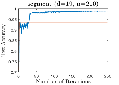
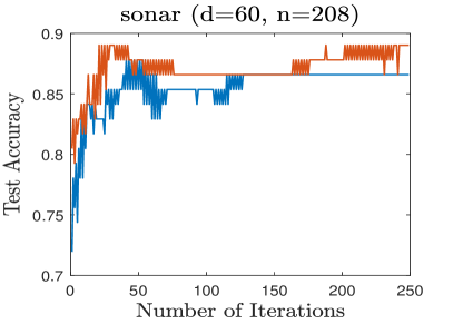
Figure 1: Performance of minimizing $F_{error}(w)$ vs. $F_{log}(w)$ via Algorithm 1.

We now turn to comparing the performance of linear classifiers obtained by optimizing the AUC function, e.g., $F(w)=F_{AUC}(w)$ defined in (14) and its approximation via pairwise hinge loss, e.g., $F(w)=F_{hinge}(w)$ as is defined in (6). The setting of the parameters and the type of the artificial and real data sets are the same as in Tables 1 and 3.

The results for artificial data sets are summarized in Table 5 as the same manner of Table 2, except that we report the AUC value as the performance measure of the resulting classifiers. As we can see in Table 5, in the process of minimizing $F_{AUC}(w)$, the only advantage of using the exact moments rather than the approximate moments is in terms of the solution time, since both approaches result in comparable average AUC values. On the other hand, the performance of the linear classifier obtained through minimizing $F_{AUC}(w)$ using approximate moments surpasses that of the classifier obtained via minimizing $F_{hinge}(w)$, both in terms of the average AUC value as well as the required solution time.

Table 5: $F_{AUC}(w)$ vs. $F_{hinge}(w)$ minimization via Algorithm 1 on artificial data sets.

Data	$\boldsymbol{F_{AUC}(w)}$ Min.		$\boldsymbol{F_{AUC}(w)}$ Min.		$\boldsymbol{F_{hinge}(w)}$ Min.
	Exact		Approximate
	moments		moments
	AUC	Time(s)	AUC	Time(s)	AUC	Time(s)
$data_{1}$	0.9972	0.01	0.9941	0.23	0.9790	5.39
$data_{2}$	0.9963	0.01	0.9956	0.22	0.9634	159.23
$data_{3}$	0.9965	0.01	0.9959	0.24	0.9766	317.44
$data_{4}$	0.9957	0.02	0.9933	0.83	0.9782	23.36
$data_{5}$	0.9962	0.02	0.9951	0.80	0.9589	110.26
$data_{6}$	0.9962	0.02	0.9949	0.82	0.9470	275.06
$data_{7}$	0.9965	0.08	0.9874	4.61	0.9587	28.31
$data_{8}$	0.9966	0.07	0.9929	4.54	0.9514	104.16
$data_{9}$	0.9962	0.08	0.9932	4.54	0.9463	157.62

Table 6 summarizes the results on real data sets, in a manner similar to Table 4, while, again using AUC of the resulting classifier as the performance measure. As we can see in Table 6, the average AUC values of the linear classifiers obtained through minimizing $F_{AUC}(w)$ and $F_{hinge}(w)$ are comparable in 14 cases out of 19, in 4 cases minimizing $F_{AUC}(w)$ performs better than minimizing $F_{hinge}(w)$ in terms of the average test AUC, while their performance is worse in the remaining 2 cases, where the algorithm stalled after a few iterations of optimizing $F_{AUC}(w)$ as is shown in Figure 2. In terms of solution time, minimizing $F_{AUC}(w)$ significantly outperforms minimizing $F_{hinge}(w)$, due to the high per-iteration complexity dependence on $n$ of $F_{hinge}(w)$ minimization.

Table 6: $F_{AUC}(w)$ vs. $F_{hinge}(w)$ minimization via Algorithm 1 on real data sets.

Data	$\boldsymbol{F_{AUC}(w)}$ Min.		$\boldsymbol{F_{hinge}(w)}$ Min.
	AUC	Time(s)	AUC	Time(s)
fourclass	0.8362	0.01	0.8362	6.81
svmguide1	0.9717	0.06	0.9863	35.09
diabetes	0.8311	0.03	0.8308	12.48
shuttle	0.9872	0.11	0.9861	2907.84
vowel	0.9585	0.12	0.9765	2.64
magic04	0.8382	0.11	0.8419	1391.29
poker	0.5054	0.11	0.5069	1104.56
letter	0.9830	0.12	0.9883	121.49
segment	0.9948	0.21	0.9992	4.23
svmguide3	0.8013	0.34	0.7877	23.89
ijcnn1	0.9269	0.08	0.9287	2675.67
german	0.7938	0.14	0.7919	32.63
landsat satellite	0.7587	0.43	0.7458	193.46
sonar	0.8214	0.88	0.8456	2.15
a9a	0.9004	0.92	0.9027	15667.87
w8a	0.9636	0.54	0.9643	5353.23
mnist	0.9943	0.64	0.9933	28410.2393
colon cancer	0.8942	2.50	0.8796	0.05
gisette	0.9957	31.32	0.9858	3280.38

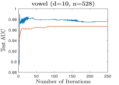
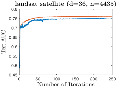
Figure 2: Performance of minimizing $F_{AUC}(w)$ vs. $F_{hinge}(w)$ via Algorithm 1.

More comprehensive numerical results are provided in the appendix, including the standard deviation of the test accuracy and test AUC.

5 Conclusion

In this work, we showed that under the Gaussian assumption, the expected prediction error and AUC of linear predictors in binary classification are smooth functions whose derivatives can be computed using the first and second moments of the related normal distribution. We then show that empirical moments of real data sets (not necessarily Gaussian) can be utilized to obtain approximate derivatives. This implies that gradient-based optimization approach can be used to optimize the prediction error and AUC function. In this work, for simplicity, we used gradient descent with backtracking line search and we demonstrated the efficiency of directly optimizing prediction error and AUC function compared to their approximations–logistic regression and pairwise hinge loss, respectively. The main advantage of these approaches is that the proposed objective functions and their derivatives are independent of the size of the data sets. Clearly more efficient second-order methods can also be utilized for optimizing these functions, which is a subject for the future research.

Appendix A Proofs of results in Section

Proof 1

(Lemma 1 proof) Note that we can split the whole set $\left\{(X,Y)~{}:~{}Y\cdot w^{T}X<0\right\}\subset\mathcal{X}\times\mathcal{Y}$ into two disjoint sets as the following:

$$\left\{(X,Y)~{}:~{}Y\cdot w^{T}X<0\right\}=\left\{(X^{+},+1)~{}:~{}w^{T}X^{+}<0\right\}\cup\left\{(X^{-},-1)~{}:~{}w^{T}X^{-}\geq 0\right\}.$$

Now, by using (7) we will have:

$$F_{error}(w)={} P\left({Y}\cdot w^{T}{X}<0\right)$$

$$={} P\left({Y}\cdot w^{T}{X}<0\cap{Y}=+1\right)+P\left({Y}\cdot w^{T}{X}<0\cap{Y}=-1\right)$$

$$={} P\left({Y}\cdot w^{T}{X}<0\mid{Y}=+1\right)P\left({Y}=+1\right)+P\left({Y}\cdot w^{T}{X}<0\mid{Y}=-1\right)P\left({Y}=-1\right)$$

$$={} P\left(w^{T}{X}^{+}<0\right)P\left({Y}=+1\right)+P\left(w^{T}{X}^{-}>0\right)P\left({Y}=-1\right)$$

$$={} P\left(w^{T}{X}^{+}\leq 0\right)P\left({Y}=+1\right)+\left(1-P\left(w^{T}{X}^{-}\leq 0\right)\right)P\left({Y}=-1\right).$$

Proof 2

(Theorem 2 proof) Let us define random variables $Z^{+}$ and $Z^{-}$ as the follows

$$Z^{+}=w^{T}{X}^{+},~{}~{}\text{and}~{}~{}Z^{-}=w^{T}{X}^{-}.$$

From (8) and using Theorem 1 we have

$${Z}^{+}\sim\mathcal{N}\left(w^{T}\mu^{+},w^{T}\Sigma^{+}w\right)~{}~{}\text{and}~{}~{}{Z}^{-}\sim\mathcal{N}\left(w^{T}\mu^{-},w^{T}\Sigma^{-}w\right).$$

Then, by using Lemma 1 we conclude the following

$$F_{error}(w) =P\left({Y}\cdot w^{T}{X}<0\right)$$

$$=\left(1-\phi\left({\mu_{Z^{+}}}/{\sigma_{Z^{+}}}\right)\right)P\left({Y}=+1\right)+\phi\left({\mu_{Z^{-}}}/{\sigma_{Z^{-}}}\right)P\left({Y}=-1\right).$$

where $\mu_{Z^{+}}=w^{T}\mu^{+}$, $\sigma_{Z^{+}}=\sqrt{w^{T}\Sigma^{+}w}$, $\mu_{Z^{-}}=w^{T}\mu^{-}$, and $\sigma_{Z^{-}}=\sqrt{w^{T}\Sigma^{-}w}$.

Proof 3

Note that based on the chain rule we have

$$\frac{d}{dw}\phi\left(f(w)\right)=\phi^{\prime}(g(w))g^{\prime}(w).$$ (15)

By substituting

$$\phi^{\prime}(x)=\frac{d}{dx}\int_{-\infty}^{x}\frac{1}{\sqrt{2\pi}}\exp\left({-\frac{1}{2}t^{2}}\right)dt=\frac{1}{\sqrt{2\pi}}\exp\left({-\frac{1}{2}x^{2}}\right)~{}~{}~{}\text{and }$$

$$g^{\prime}(w)=\frac{\sqrt{w^{T}\hat{\Sigma}w}\cdot\hat{\mu}-{\frac{w^{T}\hat{\mu}}{\sqrt{w^{T}\hat{\Sigma}w}}}\cdot\hat{\Sigma}w}{w^{T}\hat{\Sigma}w},$$

in (15) we conclude the result.

Proof 4

(Theorem 3 proof) Theorem 3 is an immediate corollary of the result of Lemma 2.

Proof 5

(Theorem 6 proof) From (10) and Theorem 5 we have

$$F_{AUC}(w) =1-P(w^{T}\left(X^{-}-X^{+})<0\right)=1-P\left(Z\leq 0\right)$$

$$=1-P\left(\frac{Z-\mu_{Z}}{\sigma_{Z}}\leq\frac{-\mu_{Z}}{\sigma_{Z}}\right)=1-\phi\left(\frac{\mu_{Z}}{\sigma_{Z}}\right),$$

where the random variable $Z$ is defined in (12), with the stated mean and standard deviation in (13).

Proof 6

(Theorem 7 proof) Theorem 7 is an immediate corollary of the result of Lemma 2, and the symmetric property of $\phi(\cdot)$.

Appendix B Numerical Analysis

The following tables summarize more comprehensive numerical comparison between minimizing $F_{error}(w)$ versus $F_{log}(w)$ and also between minimizing $F_{AUC}(w)$ versus minimizing $F_{hinge}(w)$.

Table 7: $F_{error}(w)$ vs. $F_{log}(w)$ minimization via Algorithm 1 on artificial data sets.

Data	$\boldsymbol{F_{error}(w)}$ Minimization		$\boldsymbol{F_{error}(w)}$ Minimization		$\boldsymbol{F_{log}(w)}$ Minimization
	Exact moments		Approximate moments
	Accuracy$\pm$ std	Time (s)	Accuracy $\pm$ std	Time (s)	Accuracy $\pm$ std	Time (s)
$data_{1}$	0.9965$\pm$0.0008	0.25	0.9907$\pm$0.0014	1.04	0.9897$\pm$0.0018	3.86
$data_{2}$	0.9905$\pm$0.0023	0.26	0.9806$\pm$0.0032	0.86	0.9557$\pm$0.0049	13.72
$data_{3}$	0.9884$\pm$0.0030	0.03	0.9745$\pm$0.0037	1.28	0.9537$\pm$0.0048	15.79
$data_{4}$	0.9935$\pm$0.0017	0.63	0.9791$\pm$0.0034	5.51	0.9782$\pm$0.0031	10.03
$data_{5}$	0.9899$\pm$0.0026	5.68	0.9716$\pm$0.0048	10.86	0.9424$\pm$0.0055	28.29
$data_{6}$	0.9904$\pm$0.0017	0.83	0.9670$\pm$0.0058	5.18	0.9291$\pm$0.0076	25.47
$data_{7}$	0.9945$\pm$0.0019	4.79	0.9786$\pm$0.0028	32.75	0.9697$\pm$0.0031	43.20
$data_{8}$	0.9901$\pm$0.0013	9.96	0.9290$\pm$0.0045	119.64	0.9263$\pm$0.0069	104.94
$data_{9}$	0.9899$\pm$0.0028	1.02	0.9249$\pm$0.0096	68.91	0.9264$\pm$0.0067	123.85

Table 8: $F_{error}(w)$ vs. $F_{log}(w)$ minimization via Algorithm 1 on real data sets.

Data	$\boldsymbol{F_{error}(w)}$ Minimization		$\boldsymbol{F_{log}(w)}$ Minimization
	Accuracy$\pm$ std	Time (s)	Accuracy $\pm$ std	Time (s)
fourclass	0.8782$\pm$0.0162	0.02	0.8800$\pm$0.0147	0.12
svmguide1	0.9735$\pm$0.0047	0.42	0.9506$\pm$0.0070	0.28
diabetes	0.8832$\pm$0.0186	1.04	0.8839$\pm$0.0193	0.13
shuttle	0.8920$\pm$0.0015	0.01	0.9301$\pm$0.0019	4.05
vowel	0.9809$\pm$0.0112	0.91	0.9826$\pm$0.0088	0.11
magic04	0.8867$\pm$0.0044	0.66	0.8925$\pm$0.0041	1.75
poker	0.9897$\pm$0.0008	0.17	0.9897$\pm$0.0008	10.96
letter	0.9816$\pm$0.0015	0.01	0.9894$\pm$0.0009	4.51
segment	0.9316$\pm$0.0212	0.17	0.9915$\pm$0.0101	0.36
svmguide3	0.9118$\pm$0.0136	0.39	0.8951$\pm$0.0102	0.17
ijcnn1	0.9512$\pm$0.0011	0.01	0.9518$\pm$0.0011	4.90
german	0.8780$\pm$0.0125	1.09	0.8826$\pm$0.0159	0.62
landsat satellite	0.9532$\pm$0.0032	0.01	0.9501$\pm$0.0049	3.30
sonar	0.8926$\pm$0.0292	0.49	0.8774$\pm$0.0380	0.92
a9a	0.9193$\pm$0.0021	0.98	0.9233$\pm$0.0020	11.45
w8a	0.9851$\pm$0.0005	0.36	0.9876$\pm$0.004	24.16
mnist	0.9909$\pm$0.0004	3.79	0.9938$\pm$0.0004	136.83
colon cancer	0.9364$\pm$0.0394	15.92	0.8646$\pm$0.0555	1.20
gisette	0.9782$\pm$0.0025	310.72	0.9706$\pm$0.0036	136.71

Table 9: $F_{AUC}(w)$ vs. $F_{hinge}(w)$ minimization via Algorithm 1 on artificial data sets.

Data	$\boldsymbol{F_{AUC}(w)}$ Minimization		$\boldsymbol{F_{AUC}(w)}$ Minimization		$\boldsymbol{F_{hinge}(w)}$ Minimization
	Exact moments		Approximate moments
	AUC$\pm$ std	Time (s)	AUC $\pm$ std	Time (s)	AUC $\pm$ std	Time (s)
$data_{1}$	0.9972$\pm$0.0014	0.01	0.9941$\pm$0.0027	0.23	0.9790$\pm$0.0089	5.39
$data_{2}$	0.9963$\pm$0.0016	0.01	0.9956$\pm$0.0018	0.22	0.9634$\pm$0.0056	159.23
$data_{3}$	0.9965$\pm$0.0015	0.01	0.9959$\pm$0.0018	0.24	0.9766$\pm$0.0041	317.44
$data_{4}$	0.9957$\pm$0.0018	0.02	0.9933$\pm$0.0022	0.83	0.9782$\pm$0.0054	23.36
$data_{5}$	0.9962$\pm$0.0011	0.02	0.9951$\pm$0.0013	0.80	$0.9589\pm$0.0068	110.26
$data_{6}$	0.9962$\pm$0.0013	0.02	0.9949$\pm$0.0015	0.82	0.9470$\pm$0.0086	275.06
$data_{7}$	0.9965$\pm$0.0021	0.08	0.9874$\pm$0.0034	4.61	0.9587$\pm$0.0092	28.31
$data_{8}$	0.9966$\pm$0.0008	0.07	0.9929$\pm$0.0017	4.54	0.9514$\pm$0.0051	104.16
$data_{9}$	0.9962$\pm$0.0014	0.08	0.9932$\pm$0.0020	4.54	0.9463$\pm$0.0085	157.62

Table 10: $F_{AUC}(w)$ vs. $F_{hinge}(w)$ minimization via Algorithm 1 on real data sets.

Data	$\boldsymbol{F_{AUC}(w)}$ Minimization		$\boldsymbol{F_{hinge}(w)}$ Minimization
	AUC$\pm$ std	Time (s)	AUC $\pm$ std	Time (s)
fourclass	0.8362$\pm$0.0312	0.01	0.8362$\pm$0.0311	6.81
svmguide1	0.9717$\pm$0.0065	0.06	0.9863$\pm$0.0037	35.09
diabetes	0.8311$\pm$0.0311	0.03	0.8308$\pm$0.0327	12.48
shuttle	0.9872$\pm$0.0013	0.11	0.9861$\pm$0.0017	2907.84
vowel	0.9585$\pm$0.0333	0.12	0.9765$\pm$0.0208	2.64
magic04	0.8382$\pm$0.0071	0.11	0.8419$\pm$0.0071	1391.29
poker	0.5054$\pm$0.0224	0.11	0.5069$\pm$0.0223	1104.56
letter	0.9830$\pm$0.0029	0.12	0.9883$\pm$0.0023	121.49
segment	0.9948$\pm$0.0035	0.21	0.9992$\pm$0.0012	4.23
svmguide3	0.8013$\pm$0.0420	0.34	0.7877$\pm$0.0432	23.89
ijcnn1	0.9269$\pm$0.0036	0.08	0.9287$\pm$0.0037	2675.67
german	0.7938$\pm$0.0292	0.14	0.7919$\pm$0.0294	32.63
landsat satellite	0.7587$\pm$0.0160	0.43	0.7458$\pm$0.0159	193.46
sonar	0.8214$\pm$0.0729	0.88	0.8456$\pm$0.0567	2.15
a9a	0.9004$\pm$0.0039	0.92	0.9027$\pm$0.0037	15667.87
w8a	0.9636$\pm$0.0055	0.54	0.9643$\pm$0.0057	5353.23
mnist	0.9943$\pm$0.0009	0.64	0.9933$\pm$0.0009	28410.2393
colon cancer	0.8942$\pm$0.1242	2.50	0.8796$\pm$0.1055	0.05
gisette	0.9957$\pm$0.0015	31.32	0.9858$\pm$0.0029	3280.38

Appendix C Numerical Comparison vs. LDA

In the following we provide the numerical results comparing minimizing $F_{error}(w)$ and $F_{log}(w)$ versus LDA, while using the artificial data sets as well as real data sets.

Table 11: $F_{error}(w)$ and $F_{log}(w)$ minimization via Algorithm 1 vs. LDA on artificial data sets.

Data	$\boldsymbol{F_{error}(w)}$ Minimization	$\boldsymbol{F_{error}(w)}$ Minimization	$\boldsymbol{F_{log}(w)}$ Minimization	LDA
	Exact moments	Approximate moments
	Accuracy$\pm$ std	Accuracy $\pm$ std	Accuracy $\pm$ std	Accuracy $\pm$ std
$data_{1}$	0.9965$\pm$0.0008	0.9907$\pm$0.0014	0.9897$\pm$0.0018	0.9851$\pm$0.0035
$data_{2}$	0.9905$\pm$0.0023	0.9806$\pm$0.0032	0.9557$\pm$0.0049	0.9670$\pm$0.0057
$data_{3}$	0.9884$\pm$0.0030	0.9745$\pm$0.0037	0.9537$\pm$0.0048	0.9630$\pm$0.0081
$data_{4}$	0.9935$\pm$0.0017	0.9791$\pm$0.0034	0.9782$\pm$0.0031	0.9672$\pm$0.0049
$data_{5}$	0.9899$\pm$0.0026	0.9716$\pm$0.0048	0.9424$\pm$0.0055	0.9455$\pm$0.0074
$data_{6}$	0.9904$\pm$0.0017	0.9670$\pm$0.0058	0.9291$\pm$0.0076	0.9417$\pm$0.0085
$data_{7}$	0.9945$\pm$0.0019	0.9786$\pm$0.0028	0.9697$\pm$0.0031	0.9086$\pm$0.0137
$data_{8}$	0.9901$\pm$0.0013	0.9290$\pm$0.0045	0.9263$\pm$0.0069	0.8526$\pm$0.0182
$data_{9}$	0.9899$\pm$0.0028	0.9249$\pm$0.0096	0.9264$\pm$0.0067	0.8371$\pm$0.0149

Table 12: $F_{error}(w)$ and $F_{log}(w)$ minimization via Algorithm 1 vs. LDA on real data sets.

Data	$\boldsymbol{F_{error}(w)}$ Minimization	$\boldsymbol{F_{log}(w)}$ Minimization	LDA
	Accuracy$\pm$ std	Accuracy $\pm$ std	Accuracy $\pm$ std
fourclass	0.8782$\pm$0.0162	0.8800$\pm$0.0147	0.7572$\pm$0.0314
svmguide1	0.9735$\pm$0.0047	0.9506$\pm$0.0070	0.8972$\pm$0.0159
diabetes	0.8832$\pm$0.0186	0.8839$\pm$0.0193	0.7703$\pm$0.0366
shuttle	0.8920$\pm$0.0015	0.9301$\pm$0.0019	0.9109$\pm$0.0027
vowel	0.9809$\pm$0.0112	0.9826$\pm$0.0088	0.9600$\pm$0.0224
magic04	0.8867$\pm$0.0044	0.8925$\pm$0.0041	0.7841$\pm$0.0093
poker	0.9897$\pm$0.0008	0.9897$\pm$0.0008	0.9795$\pm$0.0017
letter	0.9816$\pm$0.0015	0.9894$\pm$0.0009	0.9711$\pm$0.0029
segment	0.9316$\pm$0.0212	0.9915$\pm$0.0101	0.9617$\pm$0.0331
svmguide3	0.9118$\pm$0.0136	0.8951$\pm$0.0102	0.8238$\pm$0.0259
ijcnn1	0.9512$\pm$0.0011	0.9518$\pm$0.0011	0.9081$\pm$0.0029
german	0.8780$\pm$0.0125	0.8826$\pm$0.0159	0.7675$\pm$0.0275
landsat satellite	0.9532$\pm$0.0032	0.9501$\pm$0.0049	0.9061$\pm$0.0065
sonar	0.8926$\pm$0.0292	0.8774$\pm$0.0380	0.7622$\pm$0.0499
a9a	0.9193$\pm$0.0021	0.9233$\pm$0.0020	0.8452$\pm$0.0038
w8a	0.9851$\pm$0.0005	0.9876$\pm$0.004	0.9839$\pm$0.0012
mnist	0.9909$\pm$0.0004	0.9938$\pm$0.0004	0.9778$\pm$0.0013
colon cancer	0.9364$\pm$0.0394	0.8646$\pm$0.0555	0.8875$\pm$0.0985
gisette	0.9782$\pm$0.0025	0.9706$\pm$0.0036	0.5875$\pm$0.0207

References

- Cortes & Vapnik (1995) Cortes, C. and Vapnik, V. Support vector networks. Machine Learning, 20:273–297, 1995.
- Fisher & Sen (1994) Fisher, N. I. and Sen, P. K. The central limit theorem for dependent random variables. in The Collected Works of Wassily Hoeffding, New York:Springer-Verlag, pp. 205–213, 1994.
- Hanley & McNeil (1982) Hanley, J. A. and McNeil, B. J. The meaning and use of the area under a receiver operating characteristic (ROC) curve. Radiology, 1982.
- Hosmer & Lemeshow (2000) Hosmer, D. W. and Lemeshow, S. Applied logistic regression, second edition. 2000.
- Izenman (2013) Izenman, A. J. Modern Multivariate Statistical Techniques. Springer Texts in Statistics, 2013.
- Joachims (2006) Joachims, T. Training linear SVMs in linear time. In ACM SIGKDD, pp. 217–226, 2006.
- Mann & R.Whitney (1947) Mann, H. B. and R.Whitney, D. On a test whether one of two random variables is stochastically larger than the other. Ann. Math. Statist, 18:50–60, 1947.
- Osuna et al. (1997) Osuna, E., Freund, R., and Girosi, F. Training support vector machines: an application to face detection. In IEEE Conference on Computer Vision and Pattern Recognition, pp. 130–136, 1997.
- Rudin & Schapire (2009) Rudin, C. and Schapire, R. E. Margin-based ranking and an equivalence between adaboost and rankboost. Journal of Machine Learning Research, 10:2193–2232, 2009.
- Scholkopf et al. (1998) Scholkopf, B., Smola, A., Muller, K. R., Burges, C. J. C., and Vapnik, V. Support vector methods in learning and feature extraction. In Ninth Australian Congress on Neural Networks, 1998.
- Steck (2007) Steck, H. Hinge rank loss and the area under the ROC curve. In ECML, Lecture Notes in Computer Science, pp. 347–358, 2007.
- Tong (1990) Tong, Y.L. The multivariate normal distribution. Springer Series in Statistics, 1990.
- Yan et al. (2003) Yan, L., Dodier, R., Mozer, M.C., and Wolniewicz, R. Optimizing classifier performance via approximation to the wilcoxon-mann-witney statistic. Proceedings of the Twentieth Intl. Conf. on Machine Learning, AAAI Press, Menlo Park, CA, pp. 848–855, 2003.
- Zhao et al. (2011) Zhao, P., Hoi, S. C. H., Jin, R., and Yang, T. Online AUC maximization. In Proceedings of the 28th ICML, Bellevue, WA, USA, 2011.