Abstract

We identify the $T$-odd structure functions that appear in the description of polarized top quark decays in the sequential decay $t(\uparrow)\to X_{b}+W^{+}(\to\ell^{+}+\nu_{\ell})$ (two structure functions) and the quasi-three-body decay $t(\uparrow)\to X_{b}+\ell^{+}+\nu_{\ell}$ (one structure function). A convenient measure of the magnitude of the $T$-odd structure functions is the contribution of the imaginary part $\mathop{\rm Im}\nolimits g_{R}$ of the right-chiral tensor coupling $g_{R}$ to the $T$-odd structure functions which we work out. Contrary to the case of QCD the NLO electroweak corrections to polarized top quark decays admit of absorptive one-loop vertex contributions. We analytically calculate the imaginary parts of the relevant four electroweak one-loop triangle vertex diagrams and determine their contributions to the $T$-odd helicity structure functions that appear in the description of polarized top quark decays.

1 Introduction

Large numbers of single top quarks have been and are being currently produced at the LHC [1, 2, 3, 4]. The present situation concerning both ATLAS and CMS results on single top production is nicely summarized in a review article by N. Faltermann [5]. The dominant production mechanism is the so-called $t$-channel production process. The production proceeds via parity-violating weak interactions – a necessary condition for the top quark to be polarized. In fact, theoretical calculations predict an average polarization close to $90\%$ [6, 7] where the polarization is primarily along the direction of the spectator quark. The polarization of singly produced top quarks has been measured by the CMS Collaboration [8] ($P_{t}=0.58\pm 0.22$), by the ATLAS Collaboration [9] ($P_{t}=0.97\pm 0.12$) and, most recently, again by the ATLAS collaboration who quote a polarization value of $|\vec{P}|>0.72$ at a confidence level of $95\%$ [10].

There are two ways in which polarized top quark decays can be analyzed. In the first approach one first considers the quasi-two-body decay $t(\uparrow)\to X_{b}+W^{+}$ which is analyzed in the top quark rest frame. The subsequent decay $W^{+}\to\ell^{+}+\nu_{\ell}$ is analyzed in the $W^{+}$ rest frame. One first calculates the spin density matrix elements of the produced gauge boson $W^{+}$ in the production process $t\to X_{b}+W^{+}$ and then analyzes the spin density matrix with the help of the decay $W^{+}\to\ell^{+}+\nu_{\ell}$. The structure of the $(tbW)$ vertex has been probed in this way in a number of experimental investigations [9, 11, 12, 13]. It is clear that, in a perturbative next-to-leading order (NLO) calculation, one has to complement the (Born $\otimes$ one-loop) contributions to the spin density matrix by the integrated (tree $\otimes$ tree) contributions. In the second approach one considers the quasi-three-body decay $t(\uparrow)\to X_{b}+\ell^{+}+\nu_{\ell}$ which is analyzed entirely in the top quark rest frame.

The general matrix element for the decay $t\to b+W^{+}$ including the leading-order (LO) standard model (SM) contribution is written as [14, 15, 16, 17]

$$M_{\mu}(tbW^{+})=-\frac{g_{W}}{\sqrt{2}}\bar{u}_{b}\Big{[}\gamma_{\mu}((V_{tb}^{\ast}+f_{L})P_{L}+f_{R}P_{R})+\frac{i\sigma_{\mu\nu}\,q^{\nu}}{m_{W}}\,\Big{(}g_{L}P_{L}+g_{R}P_{R}\Big{)}\Big{]}u_{t}$$ (1)

where $P_{L,R}=(1\mp\gamma_{5})/2$. The LO SM structure of the $(tbW)$ vertex is obtained by dropping all terms except for the contribution proportional to $V^{\ast}_{tb}\sim 1$. The form factors are in general complex-valued functions where SM imaginary parts can be generated by $CP$-conserving final state interactions or can be introduced by hand as non-SM $CP$-violating imaginary contributions.

The set of observables in polarized top quark decays divide into two classes – the $T$-even and $T$-odd observables. The $T$-even observables, including their NLO QCD corrections have been discussed before in Refs. [18, 19] (sequential decays) and in Refs. [20, 21, 22, 23] (quasi-three-body decays). This paper is devoted to a detailed analysis of the $T$-odd observables contributing to polarized top quark decays. These are either fed by $CP$-conserving SM final state interactions or by $CP$-violating non-SM interactions.

The matrix element (1) is folded with the Born term contribution to obtain the relevant $T$-odd contributions. In the case $m_{b}=0$ (which we use throughout the paper) it turns out that only the coefficient $\mathop{\rm Im}\nolimits g_{R}$ generates $T$-odd correlations. $T$-odd correlations can be studied in both the sequential decay $t(\uparrow)\to X_{b}+W^{+}(\to\ell^{+}+\nu_{\ell})$ and the quasi-three-body decay $t(\uparrow)\to X_{b}+\ell^{+}+\nu_{\ell}$. In either case we count the number of $T$-odd observables, determine the angular factors that multiply them in the relevant angular decay distributions and quantify them in terms of the contribution of the imaginary part of the right-chiral tensor coupling $g_{R}$.

We discuss the two approaches in turn in Secs. 2 and 3 where we concentrate on the $T$-odd contributions to these decays. We comment on the relations between the two approaches at the end of Sec. 3. In Sec. 4 we discuss positivity constraints on the various coupling factors in Eq. (1) resulting from the requirement that the differential angular decay rate has to remain positive definite over the full angular phase space.

In Sec. 5 we discuss the electroweak contributions to $\mathop{\rm Im}\nolimits g_{R}$. Contrary to the case of QCD the NLO electroweak corrections admit absorptive one-loop vertex contributions, or, put in a different language, of final state interactions/rescattering corrections. The absorptive parts of the NLO electroweak one-loop vertex contributions treated in this paper in the case $m_{b}=0$ provide imaginary contributions to the coupling terms $f_{L}$ and $g_{R}$ where $\mathop{\rm Im}\nolimits f_{L}$ does not contribute to the $T$-odd correlations. The reason is that $f_{L}$ multiplies the same coupling structure as the Born term. The results on $\mathop{\rm Im}\nolimits g_{R}$ are presented in analytical form. The absorptive contributions to $g_{R}$ have been calculated before analytically (for photon exchange) and numerically (for $Z$ exchange) in Refs. [17] and [24]. We agree with the results of Ref. [24] up to small numerical differences but disagree with the result of Ref. [17] for the $Z$ exchange contribution. Finally, in Sec. 6 we provide a summary of our results and present our conclusions.

2 Quasi-two-body decay $t(\uparrow)\to X_{b}+W^{+}$ followed
by the decay $W^{+}\to\ell^{+}+\nu_{\ell}$ (sequential decay)

Let us begin by counting the number of independent structure functions that appear in the description of the sequential decay $t(\uparrow)\to X_{b}+W^{+}(\to\ell^{+}+\nu_{\ell})$. This is best done by considering the independent spin density matrix elements $H_{\lambda_{W}\,\lambda^{\prime}_{W}}^{\,\lambda^{\phantom{x}}_{t}\,\lambda^{\prime}_{t}}$ of the $W^{+}$ (also called helicity structure functions or, for short, structure functions) which form a hermitian $(3\times 3)$ matrix

$$\bigg{(}H_{\lambda_{W}\,\lambda^{\prime}_{W}}^{\,\lambda^{\phantom{x}}_{t}\,\lambda^{\prime}_{t}}\bigg{)}^{\dagger}=\bigg{(}H_{\lambda^{\prime}_{W}\,\lambda_{W}}^{\,\lambda^{\prime}_{t}\,\lambda_{t}}\bigg{)}$$ (2)

Since the spin of the $X_{b}$ state remains unobserved, one has the angular momentum constraint $\lambda_{t}+\lambda_{W}=\lambda^{\prime}_{t}+\lambda^{\prime}_{W}$ implying $|\lambda_{W}-\lambda^{\prime}_{W}|\leq 1$. With the above constraints one counts ten independent double spin density matrix elements:

$$H_{++}^{++},\,H_{++}^{--},\,H_{--}^{++},\,H_{--}^{--},\,H_{00}^{++},\,H_{00}^{--},\,\mathop{\rm Re}\nolimits H_{+0}^{+-},\,\mathop{\rm Im}\nolimits H_{+0}^{+-},\,\mathop{\rm Re}\nolimits H_{-0}^{-+},\,\mathop{\rm Im}\nolimits H_{-0}^{-+}.$$ (3)

The two structure functions $\mathop{\rm Im}\nolimits H_{+0}^{+-}$ and $\mathop{\rm Im}\nolimits H_{-0}^{+-}$ are so-called $T$-odd structure functions, the terminology of which will be explained later on.

In the narrow width approximation the decay $t(\uparrow)\to X_{b}+\ell^{+}+\nu_{\ell}$ can be described by a sequential two-step decay process given by the decays $t(\uparrow)\to X_{b}+W^{+}$ and $W^{+}\to\ell^{+}+\nu_{\ell}$. Accordingly one defines two coordinate systems – the top quark rest frame and the $W^{+}$ rest frame – where the repective angles in the two systems are defined in Fig. 1.

Figure 1: Definition of the polar angles $\theta$ and $\theta_{P}$ and the azimuthal angle $\phi$ in the sequential decay $t(\uparrow)\to X_{b}+W^{+}(\to\ell^{+}+\nu_{\ell})$

The $W^{+}$ produced in the decay $t(\uparrow)\to X_{b}+W^{+}$ is highly polarized. The polarization of the $W^{+}$ can be analyzed in the angular decay distribution of the decay $W^{+}\to\ell^{+}+\nu_{\ell}$. The full three-fold angular decay distribution is obtained from the trace of the product of the spin-1 density matrix of the $W^{+}$ in the production process $t\to b+W^{+}$ and the transpose of the spin-1 density matrix describing the decay process $W^{+}\to\ell^{+}+\nu_{\ell}$.

The production spin density matrix ${\cal H}_{\lambda_{W}\lambda^{\prime}_{W}}(\theta_{P})$ reads

$${\cal H}_{\lambda_{W}\lambda^{\prime}_{W}}(\theta_{P})=\left(\begin{array}[]{ccc}H_{++}+H_{++}^{P}P\cos\theta_{P}&H_{+0}^{P}\,P\sin\theta_{P}&0\\ H_{0+}^{P}P\sin\theta_{P}&H_{00}+H_{00}^{P}P\cos\theta_{P}&H_{0-}^{P}\,P\sin\theta_{P}\\ 0&H_{-0}^{P}\,P\sin\theta_{P}&H_{--}+H_{--}^{P}P\cos\theta_{P}\end{array}\right)$$ (4)

In practice one works with a normalized spin density matrix $\widehat{\cal H}_{\lambda_{W}\lambda^{\prime}_{W}}={\cal H}_{\lambda_{W}\lambda^{\prime}_{W}}/{\cal H}_{\rm tot}$ where ${\cal H}_{\rm tot}=H_{++}+H_{00}+H_{--}$. In addition, it is also useful to extract the unit matrix $1\kern-2.5pt\hbox{\rm l}$ from the normalized spin density matrix (see e.g. Ref. [25]).

The polarization of the top quark in the top quark rest frame is given by (see Fig. 1)

$$\vec{P}_{t}=P\,(\sin\theta_{P},0,\cos\theta_{P})$$ (5)

where $P$ is the magnitude of the polarization of the top quark. The relevant helicity structure functions can be projected with the help of the spin-1 polarization four-vectors of the $W^{+}$ which, in the top quark rest frame, is given by

$$\varepsilon(0)^{\mu}=\frac{1}{\sqrt{q^{2}}}(|\vec{q}|;\,0,\,0,\,q_{0})\qquad\varepsilon(\pm)^{\mu}=\frac{1}{\sqrt{2}}(0;\,\mp 1,\,-i,\,0)$$ (6)

The longitudinal and transverse polarization components of the top quark are given by $s_{t}^{\ell\,\mu}=(0;0,0,1)$ and $s_{t}^{tr\,\mu}=(0;1,0,0)$, again in the top quark rest frame. The diagonal elements ($\lambda_{W}=\lambda^{\prime}_{W}$) of ${\cal H}_{\lambda_{W}\lambda^{\prime}_{W}}$ are defined by

$${\rm diagonal\,\,unpolarized}\qquad{\cal H}_{\lambda_{W}\lambda_{W}} = {\cal H}_{\mu\,\nu}\varepsilon^{\ast\,\mu}(\lambda_{W})\varepsilon^{\nu}(\lambda_{W})$$

$${\rm diagonal\,\,polarized}\qquad{\cal H}^{P}_{\lambda_{W}\lambda_{W}} = {\cal H}_{\mu\,\nu}(s_{t}^{\ell})\varepsilon^{\ast\,\mu}(\lambda_{W})\varepsilon^{\nu}(\lambda_{W})$$ (7)

while the off-diagonal polarized elements ($\lambda_{W}\neq\lambda^{\prime}_{W}$) are determined by

$${\cal H}^{P}_{\lambda_{W}\lambda^{\prime}_{W}}={\cal H}_{\mu\,\nu}(s_{t}^{tr})\varepsilon^{\ast\,\mu}(\lambda_{W})\varepsilon^{\nu}(\lambda^{\prime}_{W})$$ (8)

Again, from angular momentum conservation one has $\lambda_{W}-\lambda^{\prime}_{W}=\pm 1=\lambda^{\prime}_{t}-\lambda_{t}$. The two configurations $(\lambda_{t}\,,\lambda^{\prime}_{t})=(1/2,-1/2),\,(-1/2,1/2)$ are associated with the transverse polarization of the top quark (for details see Ref. [19]).

The leptonic spin density matrix ${\cal L}_{\lambda_{W}\lambda^{\prime}_{W}}$ can be projected in a similar way. One obtains (see e.g. Ref. [26])

$$\!\!\!{\cal L}_{\lambda_{W}\lambda^{\prime}_{W}}(\theta,\phi)=\frac{q^{2}}{2}\times$$

$$\left(\begin{array}[]{ccc}(1+\cos\theta)^{2}&\frac{2}{\sqrt{2}}(1+\cos\theta)\sin\theta\,e^{i\phi}&\sin^{2}\theta\,e^{2i\phi}\\ \frac{2}{\sqrt{2}}(1+\cos\theta)\sin\theta\,e^{-i\phi}&2\sin^{2}\theta&\frac{2}{\sqrt{2}}(1-\cos\theta)\sin\theta\,e^{i\phi}\\ \sin^{2}\theta e^{-2i\phi}&\frac{2}{\sqrt{2}}(1-\cos\theta)\sin\theta\,e^{-i\phi}&(1-\cos\theta)^{2}\end{array}\right)$$ (12)

where the angles $\theta$ and $\phi$ are defined in Fig. 1. We have set $m_{\ell}=0$ in Eq. (2). The angular decay distribution is then obtained from [19, 25, 27, 28, 29, 30]

$$W(\theta,\theta_{P},\phi)=\sum_{\lambda_{W}\lambda^{\prime}_{W}}{\cal H}_{\lambda_{W}\lambda^{\prime}_{W}}(\theta_{P}){\cal L}_{\lambda_{W}\lambda^{\prime}_{W}}(\theta,\phi)=\mathop{\rm Tr}\nolimits\left({\cal H}(\theta_{P})\cdot{\cal L}^{T}(\theta,\phi)\right)$$ (13)

Here we concentrate on the $T$-odd correlations in the angular decay distribution (13). The $T$-odd pieces are given by the terms in Eq. (13) proportional to $\sin\phi$. One has

$$W^{T{\rm-odd}}(\theta,\theta_{P},\phi) = q^{2}\Big{(}-\sqrt{2}H_{{\cal I}I}^{P}\sin\theta_{P}\,\sin 2\theta\,\sin\phi$$ (14)

$$+2\sqrt{2}H_{{\cal I}A}^{P}\sin\theta_{P}\,\sin\theta\,\sin\phi\Big{)}$$

where we define two $T$-odd helicity structure functions by [31, 32]

$$H_{{\cal I}I}^{P} = \frac{-i}{4}\Big{(}H^{P}_{+0}-H^{P}_{0+}+H^{P}_{-0}-H^{P}_{0-}\Big{)}$$

$$H_{{\cal I}A}^{P} = \frac{-i}{4}\Big{(}H^{P}_{+0}-H^{P}_{0+}-H^{P}_{-0}+H^{P}_{0-}\Big{)}$$ (15)

Compared to Refs. [31, 32] we have changed the notation for the $T$-odd structure functions such that $(H_{5},\,H_{9})\,\to\,(H_{{\cal I}I},\,H_{{\cal I}A}$).

That the two angular factors in Eq. (14) correspond to $T$-odd correlations can be seen by representing the angular factors in Eq. (14) in terms of triple-products. To demonstrate this we collect the relevant normalized three-vectors as defined in Fig. 1. They read

$$\hat{p}_{\ell}=(\sin\theta\,\cos\phi,\sin\theta\,\sin\phi,\cos\theta)\qquad\hat{q}=(0,0,1)\qquad\hat{P}_{t}=(\sin\theta_{P},0,\cos\theta_{P})$$ (16)

One then finds

$$\sin\theta_{P}\,\sin\theta\,\sin\phi = \hat{q}\cdot(\hat{P}_{t}\times\hat{p}_{\ell})$$

$$\sin\theta_{P}\,\sin 2\theta\,\sin\phi = 2\,(\hat{p}_{\ell}\cdot\,\hat{q})\,\,\hat{q}\cdot(\hat{P}_{t}\times\hat{p}_{\ell})$$ (17)

The nomenclature $T$-odd interaction derives from the fact that a product consisting of an odd number of momenta or polarization vectors as in Eq. (17) changes sign under the time-reversal operation $t\to-t$ since the three-momentum $\vec{p}$ and the polarization vector $\vec{P}_{t}$ transform as $(\vec{p},\vec{P}_{t})\to(-\vec{p},-\vec{P}_{t})$ under $t\to-t$.

After having set up the general formalism, we are now ready to discuss the contribution of $\mathop{\rm Im}\nolimits g_{R}$ to the $T$-odd structure functions. We shall work at the leading level, i.e. we take the final state to be made up of a single bottom quark and a $W^{+}$. That is, we now deal with $t\to b+W^{+}$ instead of $t\to X_{b}+W^{+}$. We also treat the contributions of $f_{L}$, $f_{R}$, $g_{L}$ and $g_{R}$ as small perturbations. We thus keep only terms linear in $f_{L}$, $f_{R}$, $g_{L}$ and $g_{R}$ when we fold these with the SM Born term.

We further assume $m_{b}=0$. In the case $m_{b}=0$, there are a number of simplifications. For once, in the linear approximation there are no interference terms between the left-chiral Born term and the right-chiral coupling terms $f_{R}$ and $g_{L}$. This implies that the massless bottom quark contributes effectively only with its negative helicity state, i.e. $\lambda_{b}=-1/2$. This implies that $\lambda_{W}\neq 1$ due to the angular momentum constraint $\lambda_{t}=\lambda_{W}-\lambda_{b}$. It follows that the four density matrix elements $H^{P}_{+0}$, $H^{P}_{0+}$, $H_{++}$ and $H^{P}_{++}$ vanish, i.e. the hadronic double spin density matrix ${\cal H}_{\lambda_{W}\lambda^{\prime}_{W}}(\theta_{P})$ reduces to a $2\times 2$ matrix. In particular, this means that the two independent $T$-odd observables in the sequential decay $t(\uparrow)\to X_{b}+W^{+}(\to\ell^{+}+\nu_{\ell})$ coalesce to a single observable.

For $m_{b}=0$ one is effectively dealing only with two complex-valued invariant form factors in the decomposition of Eq. (1). These are the form factors $f_{L}$ and $g_{R}$. The number of independent invariant amplitudes agrees with the number of independent helicity amplitudes to which they are linearly related. The two independent helicity amplitudes are $H_{\lambda_{b}\,\lambda_{W}}=H_{-1/2\,0}\,,\,H_{-1/2\,-1}$.

Next we calculate the contribution of $\mathop{\rm Im}\nolimits g_{R}$ to the structure functions $H^{P}_{{\cal I}I}=-H^{P}_{{\cal I}A}$. The calculation can be streamlined by making use of an interesting insight provided some time ago by Kuruma [33]. For $m_{b}=0$ the longitudinal and transverse projections of the matrix element (1) are proportional to the corresponding projections of the Born term matrix elements [33]. In fact, using the covariant representation of the longitudinal polarization four-vector

$$\varepsilon^{\mu}(0)=-\,\frac{q^{2}p_{t}^{\mu}-p_{t}q\,q^{\mu}}{\sqrt{q^{2}}\sqrt{(p_{t}q)^{2}-q^{2}m_{t}^{2}}}$$ (18)

it is not difficult to see that ($x=m_{W}/m_{t}$)

$$\varepsilon^{\ast\,\mu}(0)M_{\mu}=\Big{(}1+f_{L}-x\,g_{R}\Big{)}\,\,\varepsilon^{\ast\,\mu}(0)M_{\mu}({\it Born})$$ (19)

For the transverse projection one similarly finds

$$\varepsilon^{\ast\,\mu}(-)M_{\mu}=\Big{(}1+f_{L}-\frac{1}{x}\,\,g_{R}\Big{)}\,\,\varepsilon^{\ast\,\mu}(-)M_{\mu}({\it Born})$$ (20)

where the derivation of the factorization property is facilitated by making use of the Gordon-type identity

$$\bar{u}_{b}\frac{i\sigma_{\mu\nu}q^{\nu}}{m_{W}}P_{R}u_{t}=\bar{u}_{b}\left(-\frac{1}{x}\gamma_{\mu}P_{L}+\frac{1}{x}\,\frac{(2p_{t\,\mu}-q_{\mu})}{m_{t}}P_{R}\right)u_{t}$$ (21)

To proceed we calculate the Born term spin density matrix elements of the $W^{+}$ needed when using Eqs. (19) and (20). The corresponding Born term decay tensor $B^{\mu\,\nu}$ reads

$$B^{\mu\,\nu}=\sum_{\rm spins}M^{\mu}({\it Born})M^{\dagger\,\nu}({\it Born}) = \mathop{\rm tr}\nolimits\Big{\{}p\kern-5.0pt/_{b}\gamma^{\mu}{\textstyle\frac{1}{2}}(1-\gamma_{5})(p\kern-5.0pt/_{t}+m_{t})(1+\gamma_{5}s\kern-5.5pt/_{t})\gamma^{\nu}{\textstyle\frac{1}{2}}(1-\gamma_{5})\Big{\}}$$ (22)

$$= 2\left(\bar{p}_{t}^{\mu}p_{b}^{\nu}+\bar{p}_{t}^{\nu}p_{b}^{\mu}-\bar{p}_{t}\cdot p_{b}g^{\mu\nu}-i\epsilon^{\mu\nu\alpha\beta}\bar{p}_{t\,\alpha}p_{b\,\beta}\right)$$

where $\bar{p}_{t}=p_{t}-m_{t}s_{t}$. The Born term spin density elements $B_{i}$ and $B_{i}^{P}$ have been listed in Ref. [19]. For the nondiagonal structure functions discussed here one has to specify $s_{t}^{\mu}=s_{t}^{tr\mu}=(0;1,0,0)$ (see Fig. 1). One has

$$B^{P}_{I}=-B^{P}_{A}=-\frac{1}{4}(B_{-0}+B_{0-})=-\frac{1}{2}\sqrt{2}m_{t}^{2}\frac{1-x^{2}}{x}$$ (23)

As discussed before we keep only terms linear in $f_{L}$ and $g_{R}$ when calculating the structure functions $H^{P}_{-0}$ and $H^{P}_{0-}$ assuming that the form factors are small. One has

$$H^{P}_{-0} = \Big{(}1+2\mathop{\rm Re}\nolimits f_{L}-\frac{1+x^{2}}{x}\mathop{\rm Re}\nolimits g_{R}-i\frac{1-x^{2}}{x}\mathop{\rm Im}\nolimits g_{R}\Big{)}B^{P}_{-0}$$

$$H^{P}_{0-} = \Big{(}1+2\mathop{\rm Re}\nolimits f_{L}-\frac{1+x^{2}}{x}\mathop{\rm Re}\nolimits g_{R}+i\frac{1-x^{2}}{x}\mathop{\rm Im}\nolimits g_{R}\Big{)}B^{P}_{0-}$$ (24)

The NLO imaginary contribution $\mathop{\rm Im}\nolimits f_{L}$ does not contribute to the nondiagonal matrix elements $H^{P}_{-0}=H^{P\ast}_{0-}$ because the matrix element $f_{L}$ multiplies the same covariant $\gamma_{\mu}P_{L}$ as the Born term; i.e., it is self-interfering.

For the $T$-odd structure functions one finally obtains

$${\cal H}^{P}_{{\cal I}I}=-{\cal H}^{P}_{{\cal I}A} = -\frac{i}{4}\left(H^{P}_{-0}-H^{P}_{0-}\right)\ =\ \frac{1-x^{2}}{x}\,\mathop{\rm Im}\nolimits g_{R}\,B^{P}_{I}$$ (25)

$$= -\frac{m_{t}^{2}}{\sqrt{2}}\left(\frac{1-x^{2}}{x}\right)^{2}\mathop{\rm Im}\nolimits g_{R}$$

The $m_{b}=0$ $T$-odd angular decay distribution reads

$$W^{T{\rm-odd}}(\theta,\theta_{P},\phi) = 2\sqrt{2}\,{\cal H}^{P}_{{\cal I}I}\,P_{t}\sin\theta_{P}\,\sin\theta\,(1-\cos\theta)\,\sin\phi$$ (26)

$$= -2m_{t}^{4}(1-x^{2})^{2}\mathop{\rm Im}\nolimits g_{R}P_{t}\sin\theta_{P}\,\sin\theta\,(1-\cos\theta)\,\sin\phi$$

with an overall factor $(1-\cos\theta)$ as expected from angular momentum conservation.

In order to get a feeling for the size of the $T$-odd contribution relative to the unpolarized rate we integrate the full angular decay distribution over $\cos\theta$ where we keep only the Born term contributions in the $T$-even terms. One has

$$W(\theta_{P},\phi) = \int_{-1}^{1}d\cos\theta\,\,W(\theta,\theta_{P},\phi)$$ (27)

$$= \frac{4}{3}m_{t}^{4}(1-x^{2})(1+2x^{2})\Bigg{(}1+\frac{(1-2x^{2})}{(1+2x^{2})}\cos\theta_{P}$$

$$+\frac{3}{4}\pi\frac{x}{(1+2x^{2})}\sin\theta_{P}\cos\phi-\frac{3}{4}\pi\frac{(1-x^{2})}{(1+2x^{2})}\mathop{\rm Im}\nolimits g_{R}P_{t}\sin\theta_{P}\,\sin\phi\Bigg{)}$$

The factor $3\pi(1-x^{2})/(4(1+2x^{2}))=1.29$ multiplying $\mathop{\rm Im}\nolimits g_{R}$ is sufficiently large to make an angular analysis such as Eq. (27) promising.

3 Quasi-three-body decays $t(\uparrow)\to X_{b}+\ell^{+}+\nu_{\ell}$

In this variant of possible angular decay distributions the decay $t(\uparrow)\to X_{b}+\ell^{+}+\nu_{\ell}$ is analyzed entirely in the top quark rest frame. Let us begin again by enumerating the number of structure functions that appear in the quasi-three-body decay $t(\uparrow)\to X_{b}+\ell^{+}+\nu_{\ell}$. These are the two complex matrix elements $M_{\lambda_{t}=1/2}$ and $M_{\lambda_{t}=-1/2}$ that describe the transition $t(\uparrow)\to X_{b}+\ell^{+}+\nu_{\ell}$. One thus has altogether the four structure functions $|M_{1/2}|^{2}$, $|M_{-1/2}|^{2}$, $\mathop{\rm Re}\nolimits M_{1/2}M^{*}_{-1/2}$ and $\mathop{\rm Im}\nolimits M_{1/2}M^{*}_{-1/2}$ needed to represent the decay process.

The angular decay distribution of the decay is obtained by folding the decay matrix $M_{\lambda_{t}}M^{*}_{\lambda^{\prime}_{t}}$ with the spin density matrix of the top quark, i.e. by calculating the trace $\mathop{\rm Tr}\nolimits(\rho_{\lambda_{t}\,\lambda^{\prime}_{t}}\,M_{\lambda_{t}}M^{*}_{\lambda^{\prime}_{t}})$ where the spin density matrix of the top quark is given by

$$\rho_{\lambda_{t}\,\lambda^{\prime}_{t}}=\hbox{$1\kern-2.5pt\hbox{\rm l}$}+P_{t\,z}\,\,\hbox{$\kern 2.5pt\vrule height=4.0pt\kern-2.5pt\sigma$}_{z}+P_{t\,x}\,\,\hbox{$\kern 2.5pt\vrule height=4.0pt\kern-2.5pt\sigma$}_{x}+P_{t\,y}\,\,\hbox{$\kern 2.5pt\vrule height=4.0pt\kern-2.5pt\sigma$}_{y}$$ (28)

($\hbox{$\kern 2.5pt\vrule height=4.0pt\kern-2.5pt\sigma$}_{i}$, $i=x,y,z$ are the Pauli matrices). The components of the polarization vector $\vec{P}_{t}=(P_{t\,i})$ depend on the coordinate system in which the decay is analyzed. There is a multitude of possible choices for the decay coordinate system. Two different classes of coordinate systems have been in use in the literature – the helicity system and the transversity system. In the helicity system the three final state momenta in the top quark rest frame span the $(x,z)$ plane while, in the transversity system, they span the $(x,y)$ plane. The two classes of systems are displayed in Fig. 2 together with the definition of the respective polar and azimuthal angles describing the orientation of the polarization vector of the top quark. Depending on the choice of coordinate system the polarized structure functions get toggled around among the various angular factors that multiply them. We shall discuss these two possible choices in turn. Which of the systems are being used in the experimental analysis has to be decided on the experimental expediency.

(a)(b)

Figure 2: Definition of the helicity system (left panel (a)) and the transversity system (right panel (b)) in the quasi-three-body decay $t(\uparrow)\to X_{b}+\ell^{+}+\nu_{\ell}$. The polar angles $\theta_{P}$ and $\vartheta_{P}$ and the azimuthal angles $\phi$ and $\varphi$ describe the orientation of the polarization vector $\vec{P}$ of the top quark in the two systems.

3.1 The helicity system

In the following, we limit our attention to three helicity systems where the decay plane is in the $(x,z)$ plane and the $z$-axis points into the $\ell^{+}$ direction, the $X_{b}$ direction or the $\nu_{\ell}$ direction. One further has to specify the orientation of the $x$ axis relative to the event. We thus define six coordinate systems according to

$${\rm system\,I}\, : \vec{p}_{\ell}\parallel z\,;\qquad a\,:\,p_{\nu\,x}\geq 0\qquad b\,:\,p_{X_{b}\,x}\geq 0$$

$${\rm system\,II}\, : \vec{p}_{X_{b}}\parallel z\,;\qquad a\,:\,p_{\ell\,x}\geq 0\qquad b\,:\,p_{\nu\,x}\geq 0$$

$${\rm system\,III}\, : \vec{p}_{\nu}\parallel z\,;\qquad a\,:\,p_{X_{b}\,x}\geq 0\qquad b\,:\,p_{\ell\,x}\geq 0$$ (29)

When labelling the three systems we follow the conventions of Ref. [34]. For instance, in system Ib the momenta and polarization vector read [23] (see Fig. 3)

$$p_{t} = m_{t}(1;0,0,0)$$

$$p_{\ell} = \frac{m_{t}}{2}x_{\ell}\,(1;0,0,1)$$

$$p_{\nu} = \frac{m_{t}}{2}(1-x_{\ell}+x^{2})(1;-\sin\theta_{\nu},0,\cos\theta_{\nu})$$

$$p_{b} = \frac{m_{t}}{2}(1-x^{2})(1;\sin\theta_{b},0,\cos\theta_{b})$$

$$s_{t} = (0,\sin\theta_{P}\cos\phi,\sin\theta_{P}\sin\phi,\cos\theta_{P})$$ (30)

where $x_{\ell}=2E_{\ell}/m_{t}$ is the scaled lepton energy and

$$\cos\theta_{\nu} = \frac{x_{\ell}(1-x_{\ell}+x^{2})-2x^{2}}{x_{\ell}(1-x_{\ell}+x^{2})}\qquad\sin\theta_{\nu}\ =\ \frac{2x\sqrt{(1-x_{\ell})(x_{\ell}-x^{2})}}{x_{\ell}(1-x_{\ell}+x^{2})}$$

$$\cos\theta_{b} = \frac{2x^{2}-x_{\ell}(1+x^{2})}{x_{\ell}(1-x^{2})}\qquad\sin\theta_{b}=\frac{2x}{x_{\ell}(1-x^{2})}\sqrt{(1-x_{\ell})(x_{\ell}-x^{2})}$$ (31)

For the spin density matrix of the top quark one has

$$\rho_{\lambda_{t}\,\lambda^{\prime}_{t}}=\hbox{$1\kern-2.5pt\hbox{\rm l}$}+P_{t}\cos\theta_{P}\,\hbox{$\kern 2.5pt\vrule height=4.0pt\kern-2.5pt\sigma$}_{z}+P_{t}\sin\theta_{P}\cos\phi\,\hbox{$\kern 2.5pt\vrule height=4.0pt\kern-2.5pt\sigma$}_{x}+P_{t}\sin\theta_{P}\sin\phi\,\hbox{$\kern 2.5pt\vrule height=4.0pt\kern-2.5pt\sigma$}_{y}$$ (32)

where $\theta_{P}$ and $\phi$ describe the orientation of the polarization vector of the top quark as can be read off from Fig. 2(a). We expand the $(2\times 2)$ decay matrix $M_{\lambda_{t}}M^{*}_{\lambda^{\prime}_{t}}$ along the unit matrix $1\kern-2.5pt\hbox{\rm l}$ and the three $\hbox{$\kern 2.5pt\vrule height=4.0pt\kern-2.5pt\sigma$}_{i}$ matrices. One has

$$M_{\lambda_{t}}M^{*}_{\lambda^{\prime}_{t}}={\textstyle\frac{1}{2}}\left(A\,\hbox{$1\kern-2.5pt\hbox{\rm l}$}+B\,\hbox{$\kern 2.5pt\vrule height=4.0pt\kern-2.5pt\sigma$}_{z}+C\,\hbox{$\kern 2.5pt\vrule height=4.0pt\kern-2.5pt\sigma$}_{x}+D\,\hbox{$\kern 2.5pt\vrule height=4.0pt\kern-2.5pt\sigma$}_{y}\right)$$ (33)

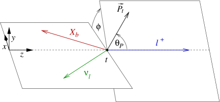
Figure 3: Definition of the polar angles $\theta_{P}$ and the azimuthal angle $\phi$ in the helicity system Ib for the quasi-three-body decay $t(\uparrow)\to X_{b}+\ell^{+}+\nu_{\ell}$

The angular decay distribution of the decay is obtained by folding the decay matrix $M_{\lambda_{t}}M^{*}_{\lambda^{\prime}_{t}}$ with the spin density matrix of the top quark, i.e. by calculating the trace $\mathop{\rm Tr}\nolimits(\rho_{\lambda_{t}\,\lambda^{\prime}_{t}}\,M_{\lambda_{t}}M^{*}_{\lambda^{\prime}_{t}})$. One obtains

$$W(\theta_{P},\phi) = \mathop{\rm Tr}\nolimits\Big{\{}\rho_{\lambda_{t}\,\lambda^{\prime}_{t}}M_{\lambda_{t}}M^{*}_{\lambda_{t}^{\prime}}\Big{\}}$$ (34)

$$= A+B\ P_{t}\cos\theta_{P}+C\ P_{t}\sin\theta_{P}\cos\phi+D\ P_{t}\sin\theta_{P}\sin\phi$$

The term proportional to the structure function $D$ represents the $T$-odd contribution as can be seen by the representation

$$\sin\theta_{P}\sin\phi=\frac{1}{\sin\theta_{\nu}}\,\hat{p}_{\nu}\cdot(\hat{p}_{\ell}\times\hat{s}_{t})$$ (35)

The structure functions $A(x_{\ell})$, $B(x_{\ell})$, $C(x_{\ell})$ and $D(x_{\ell})$ can be calculated from the contraction of the hadron and lepton tensors given by ${\cal H}^{\mu\nu}{\cal L}_{\mu\nu}$. Including the LO contribution proportional to $V_{tb}^{\ast}\sim 1$ one obtains for the six different systems

$$({\cal H}^{\mu\nu}{\cal L}_{\mu\nu})_{\rm I\,a/b}\ =\ 4m_{t}^{4}(1-x_{\ell})\Big{[}\left(x_{\ell}(1+2\mathop{\rm Re}\nolimits f_{L})-2x\mathop{\rm Re}\nolimits g_{R}\right)(1+P_{t}\cos\theta_{P})$$

$$\qquad\pm 2\sqrt{(1-x_{\ell})(x_{\ell}-x^{2})}\mathop{\rm Re}\nolimits g_{R}P_{t}\sin\theta_{P}\cos\phi$$

$$\qquad\mp 2\sqrt{(1-x_{\ell})(x_{\ell}-x^{2})}\mathop{\rm Im}\nolimits g_{R}P_{t}\sin\theta_{P}\sin\phi\Big{]}$$

$$({\cal H}^{\mu\nu}{\cal L}_{\mu\nu})_{\rm II\,a/b}\ =\ \frac{4m_{t}^{4}(1-x_{\ell})}{1-x^{2}}\Big{[}(1-x^{2})(x_{\ell}(1+2\mathop{\rm Re}\nolimits f_{L})-2x\mathop{\rm Re}\nolimits g_{R})$$

$$\qquad-\left(((1+x^{2})x_{\ell}-2x^{2})(1+2\mathop{\rm Re}\nolimits f_{L})+2x(1+x^{2}-2x_{\ell})\mathop{\rm Re}\nolimits g_{R}\right)P_{t}\cos\theta_{P}$$

$$\qquad\pm\sqrt{(1-x_{\ell})(x_{\ell}-x^{2})}\left(2x(1+2\mathop{\rm Re}\nolimits f_{L})-2(1+x^{2})\mathop{\rm Re}\nolimits g_{R}\right)P_{t}\sin\theta_{P}\cos\phi$$

$$\qquad\mp 2(1-x^{2})\sqrt{(1-x_{\ell})(x_{\ell}-x^{2})}\mathop{\rm Im}\nolimits g_{R}P_{t}\sin\theta_{P}\sin\phi\Big{]}$$

$$({\cal H}^{\mu\nu}{\cal L}_{\mu\nu})_{\rm III\,a/b}\ =\ \frac{4m_{t}^{4}(1-x_{\ell})}{1-x_{\ell}+x^{2}}\Big{[}(1-x_{\ell}+x^{2})\left(x_{\ell}(1+2\mathop{\rm Re}\nolimits f_{L})-2x\mathop{\rm Re}\nolimits g_{R}\right)$$ (36)

$$\qquad+\left(\left((1-x_{\ell}+x^{2})x_{\ell}-2x^{2}\right)(1+2\mathop{\rm Re}\nolimits f_{L})+2x(1-x_{\ell}+x^{2})\mathop{\rm Re}\nolimits g_{R}\right)P_{t}\cos\theta_{P}$$

$$\qquad\mp\sqrt{(1-x_{\ell})(x_{\ell}-x^{2})}\left(2x(1+2\mathop{\rm Re}\nolimits f_{L})-2(1-x_{\ell}+x^{2})\mathop{\rm Re}\nolimits g_{R}\right)P_{t}\sin\theta_{P}\cos\phi$$

$$\qquad\mp 2(1-x_{\ell}+x^{2})\sqrt{(1-x_{\ell})(x_{\ell}-x^{2})}\mathop{\rm Im}\nolimits g_{R}P_{t}\sin\theta_{P}\sin\phi\Big{]}.$$

After integration over $x_{\ell}$ in the limits $x^{2}\leq x_{\ell}\leq 1$ one obtains

$$\int dx_{\ell}\,\,\hbox to0.0pt{$\displaystyle({\cal H}^{\mu\nu}{\cal L}_{\mu\nu})_{\rm I\,a/b}\ =\ \frac{(1-x^{2})^{2}m_{t}^{4}}{6}\Big{[}4\left((1+2x^{2})(1+2\mathop{\rm Re}\nolimits f_{L})-6x\mathop{\rm Re}\nolimits g_{R}\right)(1+P_{t}\cos\theta_{P})$\hss}$$

$$\pm 3\pi(1-x^{2})\mathop{\rm Re}\nolimits g_{R}P_{t}\sin\theta_{P}\cos\phi\mp 3\pi(1-x^{2})\mathop{\rm Im}\nolimits g_{R}P_{t}\sin\theta_{P}\sin\phi\Big{]}$$

$$\int dx_{\ell}\,\,\hbox to0.0pt{$\displaystyle({\cal H}^{\mu\nu}{\cal L}_{\mu\nu})_{\rm II\,a/b}\ =\ \frac{(1-x^{2})^{2}m_{t}^{4}}{6}\Big{[}4\left((1+2x^{2})(1+2\mathop{\rm Re}\nolimits f_{L})-6x\mathop{\rm Re}\nolimits g_{R}\right)$\hss}$$

$$\qquad-4\left((1-2x^{2})(1+2\mathop{\rm Re}\nolimits f_{L})+2x\mathop{\rm Re}\nolimits g_{R}\right)P_{t}\cos\theta_{P}$$

$$\pm 3\pi\left(x(1+2\mathop{\rm Re}\nolimits f_{L})-(1+x^{2})\mathop{\rm Re}\nolimits g_{R}\right)P_{t}\sin\theta_{P}\cos\phi$$

$$\mp 3\pi(1-x^{2})\mathop{\rm Im}\nolimits g_{R}P_{t}\sin\theta_{P}\sin\phi\Big{]}$$

$$\int dx_{\ell}\,\,\hbox to0.0pt{$\displaystyle({\cal H}^{\mu\nu}{\cal L}_{\mu\nu})_{\rm III\,a/b}\ =\ \frac{m_{t}^{4}}{6}\Big{[}4(1-x^{2})^{2}\left((1+2x^{2})(1+2\mathop{\rm Re}\nolimits f_{L})-6x\mathop{\rm Re}\nolimits g_{R}\right)$\hss}$$ (37)

$$+4\Big{(}\left((1-x^{2})(1-11x^{2}-2x^{4})-24x^{4}\ln x\right)(1+2\mathop{\rm Re}\nolimits f_{L})$$

$$\qquad+6x(1-x^{2})^{2}\mathop{\rm Re}\nolimits g_{R}\Big{)}P_{t}\cos\theta_{P}$$

$$\mp 3\pi(1-x)^{3}\left(2x(1+3x)(1+2\mathop{\rm Re}\nolimits f_{L})-(1+x)^{3}\mathop{\rm Re}\nolimits g_{R}\right)P_{t}\sin\theta_{P}\cos\phi$$

$$\mp 3\pi(1-x^{2})^{3}\mathop{\rm Im}\nolimits g_{R}P_{t}\sin\theta_{P}\sin\phi\Big{]}$$

A few comments on the structure of the various contributions are in order.

• After azimuthal averaging and dropping the non-SM contributions $\mathop{\rm Re}\nolimits f_{L}$ and $\mathop{\rm Re}\nolimits g_{R}$ one obtains from Eq. (3.1) the well-known polar distributions

  $$W(\theta)=1+\kappa_{i}P_{t}\cos\theta\qquad{\rm with}\qquad\left\{\begin{array}[]{l}\kappa_{\rm I}=1\\ \kappa_{\rm II}=(1-2x^{2})/(1+2x^{2})=0.398\\ \kappa_{\rm III}=f(x)=-0.261\end{array}\right\}$$ (38)

  where

  $$f(x)=\frac{(1-x^{2})(1-11x^{2}-2x^{4})-24x^{4}\ln x}{(1-x^{2})^{2}(1+2x^{2})}$$ (39)

• The results of systems II and III can be obtained from the results of system I through a rotation around the $y$ axis. The relevant rotations read

  $$\left(\begin{array}[]{c}B_{\rm II}\\ C_{\rm II}\end{array}\right)=\left(\begin{array}[]{cc}\cos\theta_{b}&-\sin\theta_{b}\\ \sin\theta_{b}&\cos\theta_{b}\end{array}\right)\left(\begin{array}[]{c}B_{\rm I}\\ C_{\rm I}\end{array}\right)$$ (40)

  $$\left(\begin{array}[]{c}B_{\rm III}\\ C_{\rm III}\end{array}\right)=\left(\begin{array}[]{cc}\cos\theta_{\nu}&\sin\theta_{\nu}\\ -\sin\theta_{\nu}&\cos\theta_{\nu}\end{array}\right)\left(\begin{array}[]{c}B_{\rm I}\\ C_{\rm I}\end{array}\right)$$ (41)

  Since the unpolarized rate function $A$ and the $T$-odd $y$ component $D$ are not affected by this rotation the structure functions $A$ and $D$ are the same in all three systems such that e.g. $D_{\rm I}=D_{\rm II}=D_{\rm III}$.

• The decay distribution in system IIa is closely related to the decay distribution of sequential top quark decay discussed in Sec. 2. In fact, take Eq. (13) and substitute the relation between the cosine of the angle $\theta$ and the scaled lepton energy $x_{\ell}$ for $m_{b}=0$ (see e.g. Ref. [35])

  $$\cos\theta=\frac{(x_{\ell}-x^{2})-(1-x_{\ell})}{(1-x^{2})}\qquad\sin\theta=\frac{2}{1-x^{2}}\sqrt{(x_{\ell}-x^{2})(1-x_{\ell})}$$ (42)

  into Eq. (13). One then recovers the unintegrated distribution $({\cal H}^{\mu\nu}{\cal L}_{\mu\nu})_{\rm II\,a}$ after the replacement $\theta_{P}\to\pi-\theta_{P}$. The structure functions describing the quasi-three-body decays can be seen to be weighted sums of the unpolarized and polarized helicity structure functions in the sequential decays with weight functions $w(x_{\ell})$ that are not simple. It is only the $T$-odd structure functions that have a simple one-to-one relation. The relation between the $T$-odd structure functions ${\cal H}_{{\cal I}A}^{P}$ and $D_{\rm Ia}=D_{\rm IIa}=D_{\rm IIIa}=D_{\rm a}$ can be worked out to be

  $$D_{\rm a}=m_{t}^{2}8\sqrt{2}(1-x_{\ell})\sqrt{(1-x_{\ell})(x_{\ell}-x^{2})}\frac{x^{2}}{(1-x^{2})}\,{\cal H}_{{\cal I}A}^{P}$$ (43)

  When comparing the corresponding expressions integrated over $\cos\theta$ and $x_{\ell}$ one has to take into account the change in integration measure $d\cos\theta/dx_{\ell}=2/(1-x^{2})$.

3.2 The transversity system

The event plane is now in the $(x,y)$ plane and the $z$ axis is defined by the normal to the event plane as shown in Fig. 2(b). The angles in the helicity system and the transversity system are related by

$$\cos\vartheta_{P} = \sin\theta_{P}\sin\phi$$

$$\sin\vartheta_{P}\sin\varphi = \sin\theta_{P}\cos\phi$$

$$\sin\vartheta_{P}\cos\varphi = \cos\theta_{P}$$ (44)

These relations can be obtained by geometric reasoning or, more directly, by evaluating the scalar products $(p_{\ell}\cdot s_{t})$, $(p_{b}\cdot s_{t})$ and $\varepsilon(p_{t},p_{\ell},p_{b},s_{t})$ in the two systems using the momentum representation in helicity system Ib listed in Eq. (3.1) and the corresponding representation in the transversity system

$$p_{t} = m_{t}(1;0,0,0)$$

$$p_{\ell} = \frac{m_{t}}{2}x_{\ell}\,(1;1,0,0)$$

$$p_{\nu} = \frac{m_{t}}{2}(1-x_{\ell}+x^{2})(1;\cos\theta_{\nu},-\sin\theta_{\nu},0)$$

$$p_{b} = \frac{m_{t}}{2}(1-x^{2})(1;\cos\theta_{b},\sin\theta_{b},0)$$

$$s_{t} = (0,\sin\vartheta_{P}\cos\varphi,\sin\vartheta_{P}\sin\varphi,\cos\vartheta_{P})$$ (45)

The angular decay distribution in the transversity system can be obtained by substituting the angle relations (3.2) into the decay distribution (34). One obtains

$$W(\vartheta_{P},\varphi)=A+B\ P_{t}\sin\vartheta_{P}\cos\varphi+C\ P_{t}\sin\vartheta_{P}\sin\varphi+D\ P_{t}\cos\vartheta_{P}$$ (46)

We conclude this section by taking a closer look at the two polar correlations in helicity system I (34) and the transversity system (46) where we include also the NLO QCD corrections as listed e.g. in Ref. [36]. In helicity system I, one has

$$W(\theta_{P})\sim 1+(1-O(\Delta))\,P_{t}\cos\theta_{P}$$ (47)

where $\Delta=(\delta^{(A)}-\delta^{(B)})/(\delta^{(A)}+\delta^{(B)})=0.00178$ quantifies the NLO corrections to the LO result $\Delta=0$. The values for $\delta^{(A)}=A^{(1)}/A^{(0)}=-0.0846955$ and $\delta^{(B)}=B^{(1)}/A^{(0)}=-0.0863048$ have been taken from Ref. [36]. The NLO corrections to the LO distribution $W(\theta_{P})\sim 1+\,P_{t}\cos\theta_{P}$ in Eq. (47) can be seen to be very small even if one includes the non-SM couplings $\mathop{\rm Re}\nolimits f_{L}$ and $\mathop{\rm Re}\nolimits g_{R}$.

In the transversity system one has the polar distribution

$$W(\vartheta_{P})=1+\frac{1}{F^{(1)}(\mathop{\rm Re}\nolimits f_{L},\mathop{\rm Re}\nolimits g_{R})}\,\frac{3\pi(1-x^{2})}{4(1+2x^{2})}\,P_{t}\mathop{\rm Im}\nolimits g_{R}\cos\vartheta_{P}$$ (48)

where

$$F^{(1)}(\mathop{\rm Re}\nolimits f_{L},\mathop{\rm Re}\nolimits g_{R}) = 1+\delta^{(A)}+2\mathop{\rm Re}\nolimits f_{L}-\frac{6x}{1+2x^{2}}\mathop{\rm Re}\nolimits g_{R}$$ (49)

$$\approx (1+\delta^{(A)})\left(1+2\mathop{\rm Re}\nolimits f_{L}-\frac{6x}{1+2x^{2}}\mathop{\rm Re}\nolimits g_{R}\right)$$

$$= (1+\delta^{(A)})F^{(0)}(\mathop{\rm Re}\nolimits f_{L},\mathop{\rm Re}\nolimits g_{R})$$

The usefulness of the transversity frame polar distribution is hampered by the appearance of the unknown quantities $\mathop{\rm Re}\nolimits f_{L}$ and $\mathop{\rm Re}\nolimits g_{R}$ in the denominator of Eq. (48). As is frequently done when analyzing the impact of more than one non-SM parameters on a given decay distribution one adopts a strategy to allow one non-SM coupling at a time. For example, one can set $\mathop{\rm Re}\nolimits f_{L}=0$ and $\mathop{\rm Re}\nolimits g_{R}=0$ and keep only the non-SM coupling $\mathop{\rm Im}\nolimits g_{R}$. In this case, $F^{(1)}(\mathop{\rm Re}\nolimits f_{L},\mathop{\rm Re}\nolimits g_{R})=1+\delta^{(A)}$. One finds that the analyzing power of the distribution (48) is quite large in that $3\pi(1-x^{2})(1+\delta^{(A)})/4(1+2x^{2})=1.41$. Since the analyzing powers of both the helicity and transversity polar distributions are quite large, this two-fold set of measurements must be judged to be a very promising tool to simultaneously determine $P_{t}$ and $\mathop{\rm Im}\nolimits g_{R}$.

4 Positivity bounds in the helicity system

First observe that the structure of the differential angular decay distribution in helicity system I leaves little room for the contributions of the structure functions $C$ and $D$ if the differential rate is to remain positive definite. The LO differential decay distribution is given by

$$\frac{1}{\Gamma}\frac{d\Gamma}{d\cos\theta d\phi}=\frac{1}{4\pi}\bigg{(}A^{(0)}+B^{(0)}P_{t}\cos\theta_{P}+C^{(0)}P_{t}\sin\theta_{p}\cos\phi+D^{(0)}P_{t}\sin\theta_{p}\sin\phi\bigg{)}$$ (50)

where $A^{(0)}=B^{(0)}$ in helicity system I. The LO polar analyzing structure in helicity system I is maximal with $W(\theta_{P})\sim 1+P_{t}\cos\theta_{p}$. It is heuristically clear that for $P_{t}=1$ one can immediately conclude that the structure functions $C$ and $D$ must vanish as, in fact, is the case for the LO values of $C^{(0)}$ and $D^{(0)}$. At NLO QCD the equality of $A$ and $B$ is slightly off-set where one now has $W(\theta_{P})\sim 1+0.9982\cos\theta_{p}$ (setting again $P_{t}=1$) allowing for small contributions of $C$ and $D$.

Technically this is done by expanding $\cos\theta_{P}$ and $\sin\theta_{P}$ around $\theta_{P}=\pi$ up to second order in $\delta=\pi\pm\theta_{P}$. The vanishing of the discriminant of the corresponding quadratic equation defines the boundary of the allowed values of the coefficients of the quadratic equation.

In Ref. [36], this technique was applied to the distribution (50) to derive a positivity bound on the $T$-odd coupling factor $\mathop{\rm Im}\nolimits g_{R}$. Including contributions from $\mathop{\rm Re}\nolimits f_{L}$ and $\mathop{\rm Re}\nolimits g_{R}$, one has

$$|\mathop{\rm Im}\nolimits g_{R}|\leq\frac{4(1+2x^{2}}{3\pi(1-x^{2})}(1+\delta^{(A)})\sqrt{2\Delta(1-\Delta)}\sqrt{F^{(0)}(\mathop{\rm Re}\nolimits f_{L},\mathop{\rm Re}\nolimits g_{R})}$$ (51)

where we have used

$$1+\delta^{(B)}+2\mathop{\rm Re}\nolimits f_{L}-\frac{6x}{1+2x^{2}}\mathop{\rm Re}\nolimits g_{R}\approx(1+\delta^{(B)})\left(1+2\mathop{\rm Re}\nolimits f_{L}-\frac{6x}{1+2x^{2}}\mathop{\rm Re}\nolimits g_{R}\right)$$ (52)

For $\mathop{\rm Re}\nolimits f_{L}=\mathop{\rm Re}\nolimits g_{R}=0$ one has $F^{(0)}(\mathop{\rm Re}\nolimits f_{L},\mathop{\rm Re}\nolimits g_{R})=1$ and one recovers the bound given in Ref. [36]. As noted above, at LO one has $\Delta=0$ such that $\mathop{\rm Im}\nolimits g_{R}=0$ at LO regardless of what values $\mathop{\rm Re}\nolimits f_{L}$ and $\mathop{\rm Re}\nolimits g_{R}$ take.

Setting $\sin\phi=0$ in Eq. (50) one can derive a similar bound on the $T$-even structure function $C$. One has

$$\Big{|}\Big{(}\frac{3\pi(1-x^{2})}{4(1+2x^{2}}\mathop{\rm Re}\nolimits g_{R}-\delta^{(C)}\Big{)}\Big{|}\leq(1+\delta^{(A)})\sqrt{2\Delta(1-\Delta)}\sqrt{F^{(0)}(\mathop{\rm Re}\nolimits f_{L},\mathop{\rm Re}\nolimits g_{R})}$$ (53)

The NLO contribution $\delta^{(C)}$ to the T-even structure function $C$ appearing in Eq. (53) was calculated before in Ref. [23]. One has

$$\delta^{(C)}=\frac{C^{(1)}}{A^{(0)}} = -C_{F}\frac{\alpha_{s}}{4\pi}\frac{3}{4}\pi\frac{1}{(1-x^{2})^{2}(1+2x^{2})}\Big{\{}4x(4+3x^{2}-3x^{4})({\rm Li}_{2}(-x)-{\rm Li}_{2}(-1))$$ (54)

$$-2(1-x^{2})(8-7x+8x^{2}-5x^{3})\ln(1+x)-\frac{(1-x^{2})^{3}}{x}\ln(1-x^{2})$$

$$+2x(1-x)^{2}(1-x-2x^{2})\Big{)}\Big{\}}\ =\ -0.0024$$

As already demonstrated in Ref. [23], the NLO SM value for $\delta^{(C)}=-0.0024$ easily satisfies the SM positivity bound given by

$$|\delta^{(C)}|\leq\Big{(}1+\delta^{(A)}\Big{)}\sqrt{2\Delta(1-\Delta)}=0.0542$$ (55)

More straightforward bounds can be obtained from the various polar distributions

$$W(\theta_{P})=(1+\kappa_{i}P_{t}\cos\theta_{P})$$ (56)

in form of the constraint $|\kappa_{i}|\leq 1$ valid for $P_{t}=1$. For example, for helicity system I one finds

$$\kappa_{\rm I}=\Delta\frac{1}{F^{(1)}(\mathop{\rm Re}\nolimits f_{L},\mathop{\rm Re}\nolimits g_{R})}$$ (57)

The corresponding bound is much weaker than the bound in Eq. (51). For helicity system II one obtains ($\delta_{\rm II}^{(B)}=B_{\rm II}^{(1)}/B_{\rm II}^{(0)}$)

$$\kappa_{\rm II}=\frac{(1-2x^{2})}{(1+2x^{2})F^{(1)}(\mathop{\rm Re}\nolimits f_{L},\mathop{\rm Re}\nolimits g_{R})}\left(1+\delta_{\rm II}^{(B)}+2\mathop{\rm Re}\nolimits f_{L}+\frac{2x}{1-2x^{2}}\mathop{\rm Re}\nolimits g_{R}\right)$$ (58)

where, in system II, $\delta_{\rm II}^{(B)}=-0.12$ [18, 19]. We do not explicitely list the asymmetry parameter for helicity system III since the corresponding bound is not very illuminating. Finally, the asymmetry parameter in the transversity system reads

$$\kappa_{T}=\frac{3\pi(1-x^{2})}{4(1+2x^{2})F^{(1)}(\mathop{\rm Re}\nolimits f_{L},\mathop{\rm Re}\nolimits g_{R})}$$ (59)

Again, the bound resulting from $|\kappa_{T}|\leq 1$ is much weaker than the bound in Eq. (51).

Common to all the bounds discussed in this section is the necessity to prevent the denominator factor $F^{(1)}(\mathop{\rm Re}\nolimits f_{L},\mathop{\rm Re}\nolimits g_{R})$ from vanishing. This gives a nontrivial restriction on the parameter space $(\mathop{\rm Re}\nolimits f_{L},\mathop{\rm Re}\nolimits g_{R})$ which would, for example, further restrict the bounds on $\mathop{\rm Re}\nolimits f_{L}$ and $\mathop{\rm Re}\nolimits g_{R}$ derived from the weak radiative $B$ decays which read $-0.13<\mathop{\rm Re}\nolimits f_{L}<0.03$ and $-0.15<\mathop{\rm Re}\nolimits g_{R}<0.57$ [37].

5 Calculation of the imaginary contribution
$\mathop{\rm Im}\nolimits g_{R}$ from electroweak corrections

There are altogether 18 Feynman vertex diagrams that contribute to the decay $t\to b+W^{+}$ at NLO of the electroweak interactions. Of these 18 diagrams, seven diagrams admit absorptive parts. Three of these seven absorptive diagrams give vanishing contributions for $m_{b}=0$. One finally remains with four absorptive contributions which are depicted in Fig. 4. In the terminology of Ref. [17] the four diagrams are labeled by $(A,B,C)=(b,W,\gamma(Z))$ and $(b,\chi,\gamma(Z))$. Note that the contribution of the right diagram in Fig. 4 involving the Goldstone boson $\chi$ is needed to render the on-shell gauge boson $W^{+}$ in the left diagram to be four-transverse.

Figure 4: Absorptive parts of the four Feynman diagrams that contribute to $T$-odd correlations in polarized top quark decays

We have done a careful analysis of the absorptive parts of the diagrams in Fig. 4 and their contributions to the two invariant amplitudes $f_{L}$ and $g_{R}$. Note that there are no contributions to $f_{R}$ and $g_{L}$ in the limit $m_{b}=0$. We have found $\mathop{\rm Im}\nolimits f_{L}$ to be IR-divergent which is of no concern since $\mathop{\rm Im}\nolimits f_{L}$ does not contribute to physical observables at NLO. The reason is that $\mathop{\rm Im}\nolimits f_{L}$ multiplies the same covariance structure as the Born term. In the following we concentrate on the evaluation of $\mathop{\rm Im}\nolimits g_{R}$. The imaginary part can be extracted from the logarithms appearing in the loop calculation. As to be expected, $\mathop{\rm Im}\nolimits g_{R}$ is infrared and ultraviolet finite. The result is given by

$$\mathop{\rm Im}\nolimits g_{R}(\gamma+Z) = \frac{\alpha}{4\pi}\,\,\bigg{[}Q_{b}\,\,x(2-x^{2})-\frac{(1+2Q_{b}\sin^{2}\theta_{W})}{\sin^{2}\theta_{W}}\,\frac{1}{2x(1-x^{2})^{4}}\Big{\{}$$ (60)

$$(1-x^{2})^{2}\Big{(}x^{2}(1-x^{2})^{2}(2-x^{2})-2(1-3x^{2}-x^{4})x_{Z}^{2}\Big{)}$$

$$+\Big{(}(1-x^{2})^{2}(1-5x^{2})x_{Z}^{2}+2(1-3x^{2}-x^{4})x^{4}_{Z}\Big{)}\,\ell_{Z}\Big{\}}\bigg{]}\,\pi$$

where the numerically dominant logarithmic factor reads

$$\ell_{Z} = \ln\left(\frac{(x_{Z}^{2}+(1-x^{2})^{2})^{2}}{(x_{Z}^{2}-x^{2}(1-x^{2}))(x_{Z}^{2}+(1-x^{2})(1-2x^{2}))}\right)$$ (61)

The scaled masses of the $Z$ and $W$ boson are denoted by $x_{Z}=m_{Z}/m_{t}$ and $x=m_{W}/m_{t}$, as before. The first term in Eq. (60) proportional to $Q_{b}=-1/3$ is due to $\gamma$ exchange while the remaining contribution is due to $Z$ exchange. The analytical form of the $\gamma$-exchange contribution agrees with the corresponding result in Ref. [17] whereas the closed-form expression for the $Z$-exchange contribution in Eq. (60) is new.

Numerically one finds ($\alpha=1/128$, $\sin\theta_{W}=0.23126$, $m_{t}=173.21{\rm\,GeV}$, $m_{Z}=91.1876$, $m_{W}=80.385$ [38])

$${\rm this\,\,calculation:}\qquad\mathop{\rm Im}\nolimits g_{R}(\gamma) = -0.539\times 10^{-3}\qquad\mathop{\rm Im}\nolimits g_{R}(Z)=-1.636\times 10^{-3}$$

$$\cite[cite]{[\@@bibref{}{GonzalezSprinberg:2011kx}{}{}]}:\qquad\qquad\mathop{\rm Im}\nolimits g_{R}(\gamma) = -0.509\times 10^{-3}\qquad\mathop{\rm Im}\nolimits g_{R}(Z)=-0.726\times 10^{-3}$$

$$\cite[cite]{[\@@bibref{}{Arhrib:2016vts}{}{}]}:\qquad\qquad\mathop{\rm Im}\nolimits g_{R}(\gamma) = -0.503\times 10^{-3}\qquad\mathop{\rm Im}\nolimits g_{R}(Z)=-1.601\times 10^{-3}$$

Up to small numerical differences we agree with Refs. [17, 24] on the $\gamma$-exchange contribution and with Ref. [24] on the $Z$-exchange contribution after taking into account that we are using a running $\alpha(m_{Z}^{2})=1/128$. The present calculation on the $Z$-exchange contribution settles the factor 2 discrepancy between the results of Ref. [17] and Ref. [24] in favor of the result of Ref. [24]. The remaining small numerical differences are very likely to result from inaccurate numerical integrations in Refs. [17, 24]. Our combined result, finally, is

$$\mathop{\rm Im}\nolimits\,g_{R}(\gamma+Z)=-2.175\times 10^{-3}$$ (63)

The result on $\mathop{\rm Im}\nolimits\,g_{R}(\gamma+Z)$ is quite small. The result easily fits into the experimental bound by ATLAS [9]

$$\mathop{\rm Im}\nolimits\,g_{R}\in[-0.18,\,0.06\,]$$ (64)

and the theoretical positivity bound

$$\mathop{\rm Im}\nolimits\,g_{R}\in[-0.0420,\,0.0420\,]$$ (65)

derived in Ref. [36].

6 Summary and conclusion

We have identified the $T$-odd structure functions that appear in the description of polarized top quark decays and have written down the angular factors that multiply them in the angular decay distribution. There are two variants of angular decay distributions that have been used in the literature to describe polarized top quark decays. These are the sequential decay $t(\uparrow)\to X_{b}+W^{+}(\to\ell^{+}+\nu_{\ell})$ and the quasi-three-body decay $t(\uparrow)\to X_{b}+\ell^{+}+\nu_{\ell}$. The number of structure functions needed to describe the quasi-three-body decay is smaller than the number needed to describe the sequential decay. In this sense, the analysis of the quasi-three-body decay $t(\uparrow)\to X_{b}+\ell^{+}+\nu_{\ell}$ constitutes a more inclusive measurement than the analysis of the sequential decay $t(\uparrow)\to X_{b}+W^{+}(\to\ell^{+}+\nu_{\ell})$.

A convenient measure of the size of the $T$-odd contributions can be written down in terms of the contribution of the imaginary part of the right-chiral coupling $g_{R}$ appearing in the expansion of the general matrix element $\langle b|J_{\rm eff}|t\rangle$. Contributions to $\mathop{\rm Im}\nolimits g_{R}$ can either arise from $CP$-violating interactions for which there is no SM source or from $CP$-conserving final state interactions. In fact, within the SM there exist four NLO electroweak one-loop contributions which admit absorptive cuts. We have provided analytical and numerical results for these absorptive cuts which we present in terms of their contributions to $\mathop{\rm Im}\nolimits g_{R}$. The size of these absorptive contributions are rather small and easily fit into the existing experimental [9, 10] and theoretical [36] bounds on $\mathop{\rm Im}\nolimits g_{R}$.

We have elaborated on a possible simultaneous measurement of the polarization of the top quark and $\mathop{\rm Im}\nolimits g_{R}$ using a set of two independent polar decay distributions involving the helicity and transversity systems in the quasi-three-body decay. We have also commented on the bounds on the non-SM coupling factors that result from the positivity of the differential angular rate. To our knowledge these bounds have not been considered so far in global analysis’ of the allowed values of the non-SM coupling parameters ($\mathop{\rm Re}\nolimits f_{L}$, $\mathop{\rm Re}\nolimits g_{R}$, $\mathop{\rm Im}\nolimits g_{R}$). In our analysis we have used the $x_{\ell}$-integrated forms of the structure functions. It would be worthwhile to similarly analyze the decay distributions and bounds using the unintegrated forms of the structure functions.

We mention that when going from top quark decays to antitop quark decays one can distinguish the two sources of $CP$-violating phases. One has a phase change $e^{i\chi}\to e^{-i\chi}$ for $CP$-violating phases and no phase change $e^{i\chi}\to e^{i\chi}$ for $CP$-conserving final state interactions where we assume that the final state interactions are $CP$-conserving (see e.g. Refs. [14, 15]).

Acknowledgments

We would like to thank W. Bernreuther, R. Martinez, J. Mueller and J. Vidal for e-mail exchanges on the subject of this paper. This work was supported by the Estonian Science Foundation under Grant No. IUT2-27. S.G. acknowledges the hospitality of the theory group THEP at the Institute of Physics at the University of Mainz and the support of the Cluster of Excellence PRISMA at the University of Mainz.

References

- [1] M. Aaboud et al. [ATLAS Collaboration], JHEP 1704 (2017) 086
- [2] M. Aaboud et al. [ATLAS Collaboration], Eur. Phys. J. C77 (2017) 531
- [3] A.M. Sirunyan et al. [CMS Collaboration], Phys. Lett. B772 (2017) 752
- [4] CMS Collaboration [CMS Collaboration], “Measurement of the differential cross section for -channel single-top-quark production at ,” Report No. CMS-PAS-TOP-16-004
- [5] N. Faltermann, “Single top -channel in ATLAS and CMS,” arXiv:1709.00841 [hep-ex]
- [6] G. Mahlon and S.J. Parke, Phys. Lett. B476 (2000) 323
- [7] R. Schwienhorst, C.P. Yuan, C. Mueller and Q.H. Cao, Phys. Rev. D83 (2011) 034019
- [8] V. Khachatryan et al. [CMS Collaboration], JHEP 1604 (2016) 073
- [9] M. Aaboud et al. [ATLAS Collaboration], JHEP 1704 (2017) 124
- [10] M. Aaboud et al. [ATLAS Collaboration], JHEP 1712 (2017) 017
- [11] V. Khachatryan et al. [CMS Collaboration], JHEP 1501 (2015) 053
- [12] G. Aad et al. [ATLAS Collaboration], JHEP 1604 (2016) 023
- [13] V. Khachatryan et al. [CMS Collaboration], JHEP 1702 (2017) 028
-
[14]
W. Bernreuther, O. Nachtmann, P. Overmann and T. Schröder,
Nucl. Phys. B 388 (1992) 53; Erratum: [Nucl. Phys. B 406 (1993) 516]. - [15] W. Bernreuther, P. Gonzalez and M. Wiebusch, Eur. Phys. J. C60 (2009) 197
-
[16]
J.A. Aguilar-Saavedra, J. Carvalho, N. F. Castro, F. Veloso and A. Onofre,
Eur. Phys. J. C50 (2007) 519 -
[17]
G.A. Gonzalez-Sprinberg, R. Martinez and J. Vidal,
JHEP 1107 (2011) 094; Erratum: [JHEP 1305 (2013) 117] -
[18]
M. Fischer, S. Groote, J.G. Körner, M.C. Mauser and B. Lampe,
Phys. Lett. B451 (1999) 406 - [19] M. Fischer, S. Groote, J.G. Körner and M.C. Mauser, Phys. Rev. D65 (2002) 054036
- [20] A. Czarnecki, M. Jeżabek and J.H. Kühn, Nucl. Phys. B351 (1991) 70
-
[21]
A. Czarnecki, M. Jeżabek, J.G. Körner and J.H. Kühn,
Phys. Rev. Lett. 73 (1994) 384 - [22] A. Czarnecki and M. Jeżabek, Nucl. Phys. B427 (1994) 3
- [23] S. Groote, W.S. Huo, A. Kadeer and J.G. Körner, Phys. Rev. D76 (2007) 014012
- [24] A. Arhrib and A. Jueid, JHEP 1608 (2016) 082
- [25] J.A. Aguilar-Saavedra and J. Bernabeu, Phys. Rev. D93 (2016) 011301
- [26] T. Gutsche, M.A. Ivanov, J. G. Körner, V. E. Lyubovitskij, P. Santorelli and N. Habyl, Phys. Rev. D91 (2015) 074001; Erratum: [Phys. Rev. D91 (2015) 119907(E)]
- [27] P. Bialas, J.G. Körner, M. Krämer and K. Zalewski, Z. Phys. C57 (1993) 115
-
[28]
J.A. Aguilar-Saavedra, J. Boudreau, C. Escobar and J. Mueller,
Eur. Phys. J. C77 (2017) 200 - [29] J. Boudreau, C. Escobar, J. Mueller, K. Sapp and J. Su, “Single top quark differential decay rate formulae including detector effects,” arXiv:1304.5639 [hep-ex]
- [30] J. Boudreau, C. Escobar, J. Mueller and J. Su, J. Phys. Conf. Ser. 762 (2016) 012041
-
[31]
S. Groote and J.G. Körner,
Z. Phys. C72 (1996) 255; Erratum: [Eur. Phys. J. C70 (2010) 531] - [32] S. Groote, J.G. Körner and M.M. Tung, Z. Phys. C74 (1997) 615
- [33] T. Kuruma, Z. Phys. C57 (1993) 551
- [34] J.G. Körner and D. Pirjol, Phys. Rev. D60 (1999) 014021
- [35] A. Kadeer, J.G. Körner and U. Moosbrugger, Eur. Phys. J. C59 (2009) 27
- [36] S. Groote and J.G. Körner, Phys. Rev. D96 (2017) 111301
-
[37]
B. Grzadkowski and M. Misiak,
Phys. Rev. D78 (2008) 077501; Erratum: [Phys. Rev. D84 (2011) 059903(E)] - [38] C. Patrignani et al. [Particle Data Group], Chin. Phys. C40 (2016) 100001