Mixtures of Factor Analyzers with Fundamental Skew Symmetric Distributions

Abstract

Mixtures of factor analyzers (MFA) provide a powerful tool for modelling high-dimensional datasets. In recent years, several generalizations of MFA have been developed where the normality assumption of the factors and/or of the errors was relaxed to allow for skewness in the data. However, due to the form of the adopted component densities, the distribution of the factors/errors in most of these models is typically limited to modelling skewness concentrated in a single direction. Here, we introduce a more flexible finite mixture of factor analyzers based on the class of scale mixtures of canonical fundamental skew normal (SMCFUSN) distributions. This very general class of skew distributions can capture various types of skewness and asymmetry in the data. In particular, the proposed mixture model of SMCFUSN factor analyzers (SMCFUSNFA) can simultaneously accommodate multiple directions of skewness. As such, it encapsulates many commonly used models as special and/or limiting cases, such as models of some versions of skew normal and skew $t$-factor analyzers, and skew hyperbolic factor analyzers. For illustration, we focus on the $t$-distribution member of the class of SMCFUSN distributions, leading to mixtures of canonical fundamental skew $t$-factor analyzers (CFUSTFA). Parameter estimation can be carried out by maximum likelihood via an EM-type algorithm. The usefulness and potential of the proposed model are demonstrated using two real datasets.

1 Introduction

The factor analysis (FA) model and mixtures of factor analyzers (MFA) play a valuable role in statistical data analysis, in particular, in cluster analysis, dimension reduction, and density estimation. Their usefulness was demonstrated in a wide range of applications in different fields such as bioinformatics (McLachlan et al., 2003), informatics (Zhoe and Mobasher, 2006), pattern recognition (Yamamoto et al., 2005), social and psychological sciences (Wall et al., 2012), and environmental sciences (Maruotti et al., 2017). The traditional formulation of the MFA model assumes that the latent component factors and errors jointly follow a multivariate normal distribution. However, in applied problems, the data will not always follow the normal distribution. To allow for clusters with heavy tails, McLachlan et al. (2007) proposed the mixture of $t$-factor analyzers as a robust alternative to the MFA model, replacing the normality assumption of the factors and errors with a joint multivariate $t$-distribution.

In recent times, a number of proposals have been developed to further generalize the MFA model to incorporate other non-normal distributions for the factors and/or errors. In particular, the past decade has seen mixtures models with skew component densities gaining increasing attention, being exploited as powerful tools for handling asymmetric distributional features in heterogeneous data. To name a few, there are mixtures of skew normal distributions (Lin, 2009, Pyne et al., 2009, Kim, 2016), mixtures of skew $t$-distributions (Pyne et al., 2009, Lin, 2010, Lee and McLachlan, 2014, 2016), mixtures of the generalized hyperbolic family of distributions (Karlis and Santourian, 2009, Browne and McNicholas, 2015), and mixtures of other members of the skew elliptical class of distributions (Cabral et al., 2012). In almost all of these models, the skew component densities have the same or similar form as the skew normal distribution proposed by Azzalini and Dalla Valle (1996). Their skewness is regulated by a vector of skewness parameters multiplied by a common skewing variable in its convolution-type characterization. An implication of this type of formulation is that skewness is assumed to be concentrated along a single direction in the feature space (McLachlan and Lee, 2016) and hence referred to as a restricted skew distribution by Lee and McLachlan (2013). Another formulation of skew distributions is developed by Sahu et al. (2003), and referred to as the unrestricted skew distribution by Lee and McLachlan (2013), since it does not rely on a common skewing variable. It thus allows for skewness to be in more than one direction, although each direction is parallel to the axes of the features space. Note that the restricted model is not nested within the unrestricted model. They are, however, identical in the univariate case. The unrestricted skew normal and skew $t$-distributions were adopted for the mixture models considered by Lin (2009, 2010) and Lee and McLachlan (2014). More recently, Lee and McLachlan (2016) considered the so-called canonical fundamental skew $t$ (CFUST) distribution as components in their mixture models, a more general skew distribution that encompasses both the restricted and unrestricted formulations of skew distributions. The CFUST distribution is a member of the class of canonical fundamental skew symmetric (CFUSS) distributions proposed by Arellano-Valle and Genton (2005). As the CFUSS distribution has a matrix of skewness parameters, it can flexibly handle multiple arbitrary directions of skewness. Another member of the class of CFUSS distributions is the canonical fundamental skew hyperbolic (CFUSH) distribution, which was studied recently by Murray et al. (2017a) and Maleki et al. (2018) using different names for this distribution. A detailed treatment of skew distributions can be found in Genton (2004), Arellano-Valle and Azzalini (2006), Lee and McLachlan (2013), and Azzalini and Capitanio (2014).

A factor-analytic analogue of some of the above mentioned skew mixture models has been considered in other works, including a skew normal factor analysis model by Montanari and Viroli (2010), a mixture of skew normal factor analyzers (MSNFA) by Lin et al. (2016), a skew $t$-factor analysis by Lin et al. (2015), its mixture model version (MSTFA) by Lin et al. (2018), a mixture of (generalized hyperbolic) skew $t$-factor analyzers (MGHSTFA) by Murray et al. (2014a), and a mixture of generalized hyperbolic factor analzyers (MGHFA) by Tortora et al. (2016). There are distinct differences between these models, not only in the choice of component densities, but also on where the assumption of skewness is placed in the model (that is, whether it is assumed for the factors and/or for the errors). These will be discussed later in this paper. However, a point of interest is that the vast majority of these models adopt the restricted form of skew distributions and hence share the same limitation that the component densities are designed for modelling skewness concentrated in a single direction. Murray et al. (2017b) have recently considered a MFA model with the component errors following the unrestricted skew $t$-distribution. Such a model is suitable for the case where skewness is exhibited along the directions of the feature axes. More recently, an MFA model based on the CFUSH distribution has been considered by Murray et al. (2017c). Such a model embeds the so-called canonical fundamental skew normal (CFUSN) distribution and the unrestricted and restricted skew normal distributions as limiting cases.

In this paper, we propose a mixture of skew factor analyzers, adopting a CFUSS distribution as the joint distribution for the component factors and errors. For simplicity, we focus on the scale mixture of CFUSN (SMCFUSN) distribution. This new generalization of the MFA model can capture multiple directions of skewness simultaneously while performing implicit dimension reduction. The proposed mixture of CFUSS factor analzyers (CFUSSFA) and the mixture of SMCFUSN factor analzyers (SMCFUSNFA) also formally encompass the mixtures of skew normal, skew $t$, and the mixture of CFUSSH factor analyzers by Lin et al. (2016), Lin et al. (2018), and Murray et al. (2017b, c), respectively. For illustration, we shall focus on the $t$-distribution member of the CFUSS and SMCFUSN families of distributions, namely the canonical fundamental skew $t$ (CFUST) distribution, as it is one of the more commonly used distributions. However, it should be noted the same methodology can be applied to other members of the class of CFUSS distributions. For parameter estimation, an expectation–maximization (EM) algorithm (Dempster et al., 1977) is implemented to compute the maximum likelihood (ML) estimates of the parameters in the model. Factor scores can be obtained as part of the EM algorithm.

The rest of this paper is organised as follows. Section 2 provides a brief outline of the MFA model and the CFUSS distribution. We then examine and discuss the relationships between various existing skew factor models. In Section 3, we introduce the CFUSSFA model and present some of its nested cases. We then focus on the CFUSTFA model and implement an EM-type algorithm for parameter estimation in Section 4. Implementation details are described in Section 5. To demonstrate the usefulness of the proposed methodology, the CFUSTFA model is applied to two real datasets in Section 6. Finally, concluding remarks are given in Section 7.

2 Background and related work

2.1 Notation

We begin by establishing some notation to be used throughout this paper. Let $Y$ denote a $p$-dimensional random vector. We also let $\mbox{\boldmath$1$}_{p}$ be a $p\times 1$ vector of ones, $\mbox{\boldmath$I$}_{p}$ be the $p$-dimensional identity matrix, $\mbox{\boldmath$J$}_{p}$ be the $p\times p$ matrix of ones, and $\mathrm{𝟎}$ be a vector/matrix of appropriate size. The operator $\mbox{diag}(\cdot)$, depending on the context, produces either a diagonal matrix with the specified elements or a vector containing the diagonal elements of a diagonal matrix. The notation $|\mbox{\boldmath$y$}|$ implies taking the absolute value of each element of $y$.

The probability density function (pdf) and cumulative distribution function (cdf) of the $p$-dimensional normal distribution with mean $\mu$ and covariance $\Sigma$ are denoted by $\phi_{p}(\cdot;\mbox{\boldmath$\mu$},\mbox{\boldmath$\Sigma$})$ and $\Phi_{p}(\cdot;\mbox{\boldmath$\mu$},\mbox{\boldmath$\Sigma$})$, respectively, and the distribution itself is denoted by $N_{p}(\mbox{\boldmath$\mu$},\mbox{\boldmath$\Sigma$})$. Analogously, the pdf and cdf of a $p$-dimensional $t$-distribution with $\nu$ degrees of freedom are denoted by $t_{p}(\cdot;\mbox{\boldmath$\mu$},\mbox{\boldmath$\Sigma$},\nu)$ and $T_{p}(\cdot;\mbox{\boldmath$\mu$},\mbox{\boldmath$\Sigma$},\nu)$, respectively. When $p=1$, the subscript $p$ will be dropped for convenience of notation. The notation $TN_{p}(\cdot;\mathbb{R}^{+})$ and $Tt_{p}(\cdot;\mathbb{R}^{+})$ denote the truncated normal and $t$-distributions, respectively, that are confined to the positive hyperplane.

2.2 The class of CFUSS distributions

In many applications, the data or the clusters within the data are not symmetrically distributed. In this paper, we consider a flexible generalization of the MFA and M$t$FA models by adopting the CFUSS distribution (Arellano-Valle and Genton, 2005) for the joint distribution of the factors and errors. We begin by examining the fundamental skew distribution, one of the more general formulations of skew distributions. Its density can be expressed as the product of a symmetric density and a skewing function. Formally, the density of $Y$, a $p$-dimensional random vector following a CFUSS distribution, is given by

$$f(\mbox{\boldmath$y$};\mbox{\boldmath$\theta$}) = 2^{r}f_{p}(\mbox{\boldmath$y$};\mbox{\boldmath$\theta$})\,Q_{r}(\mbox{\boldmath$y$};\mbox{\boldmath$\theta$}),$$ (1)

where $f_{p}(\mbox{\boldmath$y$};\mbox{\boldmath$\theta$})$ is a symmetric density on $\mathbb{R}^{p}$, $Q_{r}(\mbox{\boldmath$y$};\mbox{\boldmath$\theta$})$ is a skewing function that maps $y$ into the unit interval, and $\theta$ is the vector containing the parameters of $Y$. Let $U$ be a $r\times 1$ random vector, where $Y$ and $U$ follow a joint distribution such that $Y$ has marginal density $f_{p}(\mbox{\boldmath$y$};\mbox{\boldmath$\theta$})$ and $Q_{r}(\mbox{\boldmath$y$};\mbox{\boldmath$\theta$})=P(\mbox{\boldmath$U$}>\mbox{\boldmath$0$}\mid\mbox{\boldmath$Y$}=\mbox{\boldmath$y$})$. If the latent random vector $U$ has its canonical distribution (that is, with mean $\mathrm{𝟎}$ and scale matrix $\mbox{\boldmath$I$}_{r}$), we obtain the canonical form of (1), namely the CFUSS distribution. The class of CFUSS distributions encapsulates many existing distributions, including most of those mentioned earlier in this paper. We shall consider some particular cases of the class of CFUSS distributions here.

2.2.1 The CFUSN distribution

The skew normal member of the class of CFUSS distributions is the canonical fundamental skew normal (CFUSN) distribution. This can be obtained by taking $f_{p}$ to be a normal density, leading to $Q_{r}$ being a normal cdf. It follows that the density of the CFUSN distribution is given by

$$f_{\mbox{\tiny{CFUSN}}}(\mbox{\boldmath$y$};\mbox{\boldmath$\mu$},\mbox{\boldmath$\Sigma$},\mbox{\boldmath$\Delta$}) = 2^{r}\phi_{q}(\mbox{\boldmath$y$};\mbox{\boldmath$\mu$},\mbox{\boldmath$\Omega$})\;\Phi_{r}\left(\mbox{\boldmath$\Delta$}^{T}\mbox{\boldmath$\Omega$}^{-1}(\mbox{\boldmath$y$}-\mbox{\boldmath$\mu$});\mbox{\boldmath$0$},\mbox{\boldmath$\Lambda$}\right),$$ (2)

where $\mbox{\boldmath$\Omega$}=\mbox{\boldmath$\Sigma$}+\mbox{\boldmath$\Delta$}\mbox{\boldmath$\Delta$}^{T}$ and $\mbox{\boldmath$\Lambda$}=\mbox{\boldmath$I$}_{r}-\mbox{\boldmath$\Delta$}^{T}\mbox{\boldmath$\Omega$}^{-1}\mbox{\boldmath$\Delta$}$. In the above, $\mu$ is a $p\times 1$ vector of location parameters, $\Sigma$ is a $p\times p$ positive definite scale matrix, and $\Delta$ is a $p\times r$ matrix of skewness parameters. We shall adopt the notation $\mbox{\boldmath$Y$}\sim\mbox{CFUSN}_{p,r}(\mbox{\boldmath$\mu$},\mbox{\boldmath$\Sigma$},\mbox{\boldmath$\Delta$})$ if $Y$ has the density given by (2). Note that when $\mbox{\boldmath$\Delta$}=\mbox{\boldmath$0$}$, we obtain the (multivariate) normal distribution. In addition, a number of skew normal distributions are nested within the CFUSN distribution, including the version proposed by Azzalini and Dalla Valle (1996) and the version proposed by Sahu et al. (2003). We shall follow the terminology of Lee and McLachlan (2013) and refer to them as the restricted and unrestricted skew normal distribution, respectively.

It is of interest to note that $Y$ admits a convolution-type stochastic representation that facilitates the derivation of properties and parameter estimation via the EM algorithm. This is given by

$$Y = \mbox{\boldmath$\mu$}+\mbox{\boldmath$\Delta$}|\mbox{\boldmath$U$}|+\mbox{\boldmath$e$},$$ (3)

where $U$ follows a standard $r$-dimensional normal distribution, independently of $\mbox{\boldmath$e$}\sim N_{p}(\mbox{\boldmath$0$},\mbox{\boldmath$\Sigma$})$. Hence, $|\mbox{\boldmath$U$}|$ has a standard half-normal distribution.

2.2.2 Scale mixture of CFUSN distributions

In the next two subsections, we shall consider two skew distributions that were recently employed by Lee and McLachlan (2016) and Murray et al. (2017a) for their mixture models, namely the CFUST and HTH distributions, respectively. They are special cases of the class of the CFUSS distributions that can be obtained as a scale mixture of the CFUSN (SMCFUSN) distribution. By a normal scale mixture, we mean a distribution that can be defined by the stochastic representation

$$Y = \mbox{\boldmath$\mu$}+W^{\frac{1}{2}}\mbox{\boldmath$Y$}_{0},$$ (4)

where $\mbox{\boldmath$Y$}_{0}$ follows a central CFUSN distribution and $W$ is a positive (univariate) random variable independent of $\mbox{\boldmath$Y$}_{0}$. Thus, conditional on $W=w$, the density of $Y$ is a CFUSN distribution with scale matrix ${w}\mbox{\boldmath$\Sigma$}$. It follows that the marginal density of $Y$ is given by

$$f_{\mbox{\tiny{SMCFUSN}}}(\mbox{\boldmath$y$};\mbox{\boldmath$\mu$},\mbox{\boldmath$\Sigma$},\mbox{\boldmath$\Delta$};F_{\mbox{\boldmath$\zeta$}}) = 2^{r}\int_{0}^{\infty}\phi_{p}\left(\mbox{\boldmath$y$};\mbox{\boldmath$\mu$},{w}\mbox{\boldmath$\Omega$}\right)\,\Phi_{r}\left(\frac{1}{\sqrt{w}}\mbox{\boldmath$\Delta$}^{T}\mbox{\boldmath$\Omega$}^{-1}(\mbox{\boldmath$y$}-\mbox{\boldmath$\mu$});\mbox{\boldmath$0$},\mbox{\boldmath$\Lambda$}\right)dF_{\mbox{\boldmath$\zeta$}}(w),$$

where $F_{\mbox{\boldmath$\zeta$}}$ denotes the distribution function of $W$ indexed by the parameter $\zeta$. We shall use the notation $\mbox{\boldmath$Y$}\sim SMCFUSN_{p,r}(\mbox{\boldmath$\mu$},\mbox{\boldmath$\Sigma$},\mbox{\boldmath$\Delta$};F_{\mbox{\boldmath$\zeta$}})$ if the density of $Y$ can be expressed in the form of (LABEL:SMSN). The class of SMCFUSN distributions is a generalization of the scale mixture of skew normal (SMSS) distributions considered by Cabral et al. (2012). The latter adopts a restricted skew normal distribution in place of the CFUSN distribution here. This class can be obtained from the SMCFUSN distribution by taking $r=1$ (after reparameterization). Some special cases of the SMCFUSN distribution are listed in Table 1.

Model	Notation	Scaling density	Symmetric density	Skewing function
skew hyperbolic∗	CFUSH∗	$GIG(\psi,\chi,\lambda)$	symmetric GH	symmetric GH
skew $t$	CFUST	$\mbox{invGamma}(\frac{\nu}{2},\frac{\nu}{2})$	$t$	$t$
skew normal	CFUSN	1	normal	normal
$t$	$t$	$\mbox{invGamma}(\frac{\nu}{2},\frac{\nu}{2})$	$t$	1
normal	N	1	normal	1

Table 1: Some special cases of the scale mixture of CFUSN distributions. We let CFUS denote the canonical fundamental skew distribution, SH the specialized hyperbolic distribution, and invGamma the inverse Gamma distribution. ^∗The CFUSH distribution is not identifiable and hence Murray et al. (2017a) and Maleki et al. (2018) imposed different constraints on the parameters to achieve identifiability.

2.2.3 The CFUSH distribution

If the latent variable $W$ in (4) follows a generalized inverse Gaussian (GIG) distribution (Seshadri, 1997), we obtain the canonical fundamental skew hyperbolic (CFUSH) distribution. In this case, the symmetric density $f_{p}$ in (1) is a symmetric GH distribution $h_{p}(\cdot)$ and the skewing function becomes the cdf of a symmetric GH distribution $H_{r}(\cdot)$. The GIG density can be expressed as

$$f_{\mbox{\tiny{GIG}}}(w;\psi,\chi,\lambda) = \frac{\left(\frac{\psi}{\chi}\right)^{\frac{\lambda}{2}}w^{\lambda-1}}{2K_{\lambda}(\sqrt{\chi\psi})}e^{-\frac{\psi w+\frac{\chi}{w}}{2}},$$ (6)

where $W>0$, the parameters $\psi$ and $\chi$ are positive, and $\lambda$ is a real parameter. In the above, $K_{\lambda}(\cdot)$ denotes the modified Bessel function of the third kind of order $\lambda$. The density of a $p$-dimensional symmetric generalized hyperbolic distribution is given by

$$h_{p}(\mbox{\boldmath$y$};\mbox{\boldmath$\mu$},\mbox{\boldmath$\Sigma$},\mbox{\boldmath$\psi$},\chi,\lambda) = \left(\frac{\chi+\eta}{\psi}\right)^{\frac{\lambda}{2}-\frac{p}{4}}\frac{\left(\frac{\psi}{\chi}\right)^{\frac{\lambda}{2}}K_{\lambda-\frac{p}{2}}(\sqrt{(\chi+\eta)\psi})}{(2\pi)^{\frac{p}{2}}|\mbox{\boldmath$\Sigma$}|^{\frac{1}{2}}K_{\lambda}(\sqrt{\chi\psi})}.$$ (7)

It is well known that the GH distribution has an identifiability issue in that the parameter vectors $\mbox{\boldmath$\theta$}=(\mbox{\boldmath$\mu$},c\mbox{\boldmath$\Sigma$},c\psi,\chi/c,\lambda)$ and $\mbox{\boldmath$\theta$}^{*}=(\mbox{\boldmath$\mu$},\mbox{\boldmath$\Sigma$},\psi,\chi,\lambda)$ both yield the same symmetric GH distribution (7) for any $c>0$. It is therefore not surprising that the CFUSH distribution also suffers from such an issue. To handle this, restrictions are imposed on some of the parameters of the CFUSH distribution. An example is the HTH distribution considered by Murray et al. (2017a), where the constraint $\psi=\chi=\omega$ is used, leading to the density

$$f_{\mbox{\tiny{CFUSSH}}}(\mbox{\boldmath$y$};\mbox{\boldmath$\mu$},\mbox{\boldmath$\Sigma$},\mbox{\boldmath$\Delta$},\omega,\lambda)$$

$$=2^{r}h_{p}\left(\mbox{\boldmath$y$};\mbox{\boldmath$\mu$},\mbox{\boldmath$\Omega$},\omega,\omega,\lambda\right)H_{r}\left(\mbox{\boldmath$\Delta$}^{T}\mbox{\boldmath$\Omega$}^{-1}(\mbox{\boldmath$y$}-\mbox{\boldmath$\mu$})\left(\frac{\omega}{\omega+\eta}\right)^{\frac{1}{4}};\mbox{\boldmath$0$},\mbox{\boldmath$\Lambda$},\lambda-\textstyle\frac{p}{2},\gamma,\gamma\right),$$

(8)

where $\gamma=\sqrt{\psi(\omega+\eta)}$. This particular parameterization is refer to as the canonical fundamental skew specialized hyperbolic (CFUSSH) distribution. Note that in their terminology, they are using ‘hidden truncation’ to describe the latent skewing variable that follows a truncated distribution in the convolution-type characterization of the CFUSH distribution. Another alternative is to restrict the parameters of $W$ so that, for example, $E(W)=1$. A commonly used constraint on the GH distribution is to set $|\mbox{\boldmath$\Sigma$}|=1$. This can be applied to the CFUSH distribution to achieve identifiability; see also the unrestricted skew normal generalized hyperbolic (SUNGH) distribution considered by Maleki et al. (2018).

2.2.4 The CFUST distribution

The CFUST distribution is the skew $t$-distribution member of the class of CFUSS distributions, where the symmetric distribution is taken to be a (multivariate) $t$-distribution. This can be obtained by letting $\frac{1}{W}$ be a random variable that has a $\mbox{gamma}(\frac{\nu}{2},\frac{\nu}{2})$ distribution. Thus, its density is given by

$$f_{\mbox{\tiny{CFUST}}}(\mbox{\boldmath$y$};\mbox{\boldmath$\mu$},\mbox{\boldmath$\Sigma$},\mbox{\boldmath$\Delta$},\nu)$$

$$= 2^{r}t_{p}(\mbox{\boldmath$y$};\mbox{\boldmath$\mu$},\mbox{\boldmath$\Omega$},\nu)T_{r}\left(\mbox{\boldmath$\Delta$}^{T}\mbox{\boldmath$\Omega$}^{-1}(\mbox{\boldmath$y$}-\mbox{\boldmath$\mu$});\mbox{\boldmath$0$},\left(\frac{\nu+\eta}{\nu+p}\right)\mbox{\boldmath$\Lambda$},\nu+p\right).$$

We shall adopt the notation $\mbox{\boldmath$Y$}\sim\mbox{CFUST}_{p,r}(\mbox{\boldmath$\mu$},\mbox{\boldmath$\Sigma$},\mbox{\boldmath$\Delta$},\nu)$ if $Y$ has the density given by (LABEL:CFUST).

The CFUST distribution can be represented by a number of stochastic representations, including the convolution of a half $t$-random vector $|\mbox{\boldmath$U$}|$ and a $t$-random vector $e$, given by

$$Y = \mbox{\boldmath$\mu$}+\mbox{\boldmath$\Delta$}|\mbox{\boldmath$U$}|+\mbox{\boldmath$e$},$$ (10)

where $U$ and $e$ have a joint $t$-distribution given by

$$\left[\begin{array}[]{c}\mbox{\boldmath$U$}\\ \mbox{\boldmath$e$}\end{array}\right] \sim t_{r+p}\left(\left[\begin{array}[]{c}\mbox{\boldmath$0$}\\ \mbox{\boldmath$0$}\end{array}\right],\left[\begin{array}[]{cc}\mbox{\boldmath$I$}_{r}&\mbox{\boldmath$0$}\\ \mbox{\boldmath$0$}&\mbox{\boldmath$\Sigma$}\end{array}\right],\nu\right).$$ (17)

From (10), we can obtain the mean and covariance matrix $X$, which are given by

$$E(\mbox{\boldmath$Y$}) = \mbox{\boldmath$\mu$}+a(\nu)\mbox{\boldmath$\Delta$}\mbox{\boldmath$1$}_{r}$$

and

$$\mbox{cov}(\mbox{\boldmath$Y$}) = (\frac{\nu}{\nu-2})\left[\mbox{\boldmath$\Sigma$}+\left(1-\frac{2}{\pi}\right)\mbox{\boldmath$\Delta$}\mbox{\boldmath$\Delta$}^{T}\right]+\left[\frac{2\nu}{\pi(\nu-2)}+a(\nu)^{2}\right]\mbox{\boldmath$\Delta$}\mbox{\boldmath$J$}_{r}\mbox{\boldmath$\Delta$}^{T},$$

where $a(\nu)=\sqrt{\frac{\nu}{2}}\Gamma(\frac{\nu-1}{2})\left[\Gamma(\frac{\nu}{2})\right]^{-1}$.

In addition to the CFUSN distribution (and its nested special/limiting cases), the CFUST distribution embeds a number of commonly used distributions as special or limiting cases. This includes the unrestricted $t$-distribution by Sahu et al. (2003) (obtained by taking $\Delta$ to be a diagonal $p\times p$ matrix, and letting $\nu\rightarrow\infty$ for the skew normal case), the restricted skew $t$-distributions (obtained by setting $r=1$), and the $t$-distribution (obtained by setting $\mbox{\boldmath$\Delta$}=0$). Concerning the identifiability of the CFUST model, it can be observed from (10) that it bears a resemblance to the FA model (18). Indeed, it can be viewed as a FA model with latent factors following a half $t$-distribution and the skewness matrix acting as the factor loading matrix. However, unlike the FA model, the term $\mbox{\boldmath$\Delta$}|\mbox{\boldmath$U$}|$ in the CFUST distribution is not rotational invariant. However, it is invariant to permutations of the columns of $\Delta$, but this does not affect the number of free parameters in the CFUST model.

2.3 Factor analysis (FA) and mixture of factor analyzers (MFA)

The factor analysis (FA) model postulates that the correlations between the variables in $Y$ can be explained by the linear dependence of $Y$ on a lower-dimensional latent factor $X$, as given by

$$\mbox{\boldmath$Y$}=\mbox{\boldmath$\mu$}+\mbox{\boldmath$B$}\mbox{\boldmath$X$}+\mbox{\boldmath$\epsilon$},$$ (18)

where $B$ is a $p\times q$ matrix of factor loadings, $X$ is a $q$-dimensional latent factor ($q\leq p$), and $\epsilon$ is a $p\times 1$ vector of error variables. In the traditional case of a normal MFA model, it is assumed that $\mbox{\boldmath$X$}\sim N_{q}(\mbox{\boldmath$0$},\mbox{\boldmath$I$}_{q})$ and $\mbox{\boldmath$\epsilon$}\sim N_{p}(\mbox{\boldmath$0$},\mbox{\boldmath$D$})$, and that they are independently distributed of each other. Also, $D$ is taken to be a diagonal matrix with diagonal elements given by $d$; that is, $\mbox{\boldmath$D$}=\mbox{diag(\mbox{\boldmath$d$})}$. This follows from the assumption that the variables in $Y$ are distributed independently after allowing for the factors. From (18), the marginal density of $Y$ is given by $N_{p}(\mbox{\boldmath$\mu$},\mbox{\boldmath$B$}\mbox{\boldmath$B$}^{T}+\mbox{\boldmath$D$})$. In the case of multivariate latent factors (that is, $q>1$), the FA model suffers from an identifiability issue due to the rotational invariance of $B$$U$. To ensure the FA model can be uniquely defined, $q(q-1)/2$ constraints can be imposed on the factor loadings $B$ to reduce the number of free parameters for the covariance matrix from $\frac{1}{2}p(p+1)$ to $p+pq-\frac{1}{2}q(q-1)$.

The mixture of factor analzyers (MFA) model (Ghahramani and Hinton, 1997, McLachlan and Peel, 2000) is a mixture version of the FA model wherein, given that $Y$ belongs to the $i$th component of the mixture model, it can be the expressed in the form of (18). The density of MFA is given by

$$f(\mbox{\boldmath$y$};\mbox{\boldmath$\Psi$})=\sum_{i=1}^{g}\pi_{i}f_{i}(\mbox{\boldmath$y$};\mbox{\boldmath$\theta$}_{i}),$$ (19)

where the $\pi_{i}$ $(i=1,\ldots,g)$ denote the mixing proportions, which are non-negative and sum to one. The generic function $f_{i}(\cdot)$ denotes the density of the $i$th component of the mixture model with parameters $\mbox{\boldmath$\theta$}_{i}$. In the case of the classical (normal) MFA model, this comprises the mean vectors $\mbox{\boldmath$\mu$}_{i}$, the loading matrices $\mbox{\boldmath$B$}_{i}$, and the scale matrices $\mbox{\boldmath$D$}_{i}$.

McLachlan et al. (2007) proposed the mixture of $t$-factor analysers (M$t$FA) as a more robust version of the MFA model. It is defined in a similar way to (18), but assuming that the factors and the errors jointly follow a multivariate $t$-distribution. More formally, we have

$$\mbox{\boldmath$Y$}_{j}=\mbox{\boldmath$\mu$}_{i}+\mbox{\boldmath$B$}_{i}\mbox{\boldmath$X$}_{ij}+\mbox{\boldmath$\epsilon$}_{ij},\hskip 28.45274pt\mbox{with probability }\pi_{i},$$ (20)

where

$$\left[\begin{array}[]{c}\mbox{\boldmath$X$}_{ij}\\ \mbox{\boldmath$\epsilon$}_{ij}\end{array}\right] \sim t_{q+p}\left(\left[\begin{array}[]{c}\mbox{\boldmath$0$}\\ \mbox{\boldmath$0$}\end{array}\right],\left[\begin{array}[]{cc}\mbox{\boldmath$I$}_{q}&\mbox{\boldmath$0$}\\ \mbox{\boldmath$0$}&\mbox{\boldmath$D$}_{i}\end{array}\right],\nu_{i}\right).$$ (27)

In this case, the marginal density of $\mbox{\boldmath$Y$}_{j}$ is $\sum_{i=1}^{g}\pi_{i}\,t_{p}(\mbox{\boldmath$\mu$}_{i},\mbox{\boldmath$B$}_{i}\mbox{\boldmath$B$}_{i}^{T}+\mbox{\boldmath$D$}_{i},\nu_{i})$. The M$t$FA model has the same identifiability problem as the MFA model and thus the same constraints on the factor loadings can be imposed.

2.4 Related models

As discussed in the aforementioned sections, there are a number of existing proposals for skew factor analysis models or mixtures of skew factor analyzers. They differ in (i) how the adopted skew distribution is characterized and (ii) whether it is the factors or the errors (or both) that are assumed to follow the chosen skew distribution. In this discussion, we shall focus on the more relevant models that are mentioned in Section LABEL:intro.

Concerning (ii), for the case of a single factor analysis model, Montanari and Viroli (2010) considered the restricted skew normal distribution for its factors. Kim et al. (2016) proposed the so-called generalised skew normal factor model which is equivalent to a FA model with the errors following a CFUSN distribution. In the case of mixtures of skew factor analyzers, we note that for the MSNFA and MSTFA models (Lin et al., 2016, 2018) the factors follow a (restricted) skew normal and skew $t$-distribution, respectively. In contrast, for the MGHSTFA and MGHFA models (Murray et al., 2014a, Tortora et al., 2016), the errors are assumed to follow a GHST distribution and a (special case) of the generalized hyperbolic (GH) distribution, respectively. Similarly, the model by Murray et al. (2017b) assumes that the errors follow the skew $t$-distribution by Sahu et al. (2003), which we shall refer to as the unrestricted skew $t$-factor analyzers (MuSTFA) model (following the terminology of Lee and McLachlan (2013)) to distinguish it from the other skew $t$-factor analyzers models considered in this paper. The more recent HTHFA model proposed by Murray et al. (2017c) assumes that the factors follow a CFUSSH distribution and the errors marginally follow a hyperbolic distribution. As discussed previously, we shall henceforth refer to it as the CFUSSHFA model.

Concerning (i), it should be noted that although also called the skew $t$-distribution by Murray et al. (2014a), the GHST distribution is different from the restricted skew $t$-distribution. The former arises as a special case of the GH distribution and so exhibits different tail behaviour to the restricted skew $t$-distribution. Moreover, it does not incorporate a skew normal distribution as it becomes the (symmetric) normal distribution as the degrees of freedom approach infinity. The GH distribution adopted by the GHFA model has restrictions placed on some of its parameters (similar to that for the CFUSSH distribution) due to an identifiability issue. For ease of reference, a summary of the above mentioned MFA models is listed in Table 2. Note that for brevity this list is not exhaustive and only the most relevant models are included.

A detailed study of the analytical differences between these distributions is beyond the scope of this paper. However, it is of interest here to recognize that although formulated differently, the skewness in these approaches (with the exception of uMSTFA and CFUSSHFA) is regulated by a single latent skewing variable and thus, in effect, is somewhat similar to the special case of $r=1$ of the proposed CFUSSFA and CFUSTFA models. This implies realizations of the skewing variable are confined to lie about a line in the feature space and therefore are limited to modelling skewness concentrated along a single direction (McLachlan and Lee, 2016). In the case of the uMSTFA model, there are $q$ skewing variables that are uncorrelated and taken to be feature-specific. On the other hand, the CFUSS distribution allows for $r$ latent skewness variables which enables it to represent skewness along multiple arbitrary directions.

The practical implications of this issue can be illustrated on the Wisconsin Diagnostic Breast Cancer (WDBC) dataset (Lichman, 2013). Consider the subset consisting of two variables, namely, the mean number of concave points and the standard error of the number of concave points. A scatterplot of the observations from benign patients is shown in Figure 1(a). The distribution of observations is apparently highly asymmetric and seems to exhibit skewness in two distinct directions. Upon fitting a restricted SN distribution to the data, we observed from Figure 1(c) that it successfully captures one of the skewness directions but is having difficulty with the other (see the lower left corner of the Figure). The GH distribution also finds this situation challenging to model (Figure 1(d)). The CFUSN distribution (Figure 1(b)) provides a much closer fit to the data and is capable of modelling both directions of skewness (Figure 1(a)).

Skew MFA Model	Notation	Factors	Errors	References
Restricted skew normal	MSNFA	rMSN	normal	Lin et al. (2016)
Restricted skew $t$	MSTFA	rMST	$t$	Lin et al. (2018)
Unrestricted skew $t$	uMSTFA	$t$	uMST	Murray et al. (2017b)
Generalized hyperbolic*	MGHFA	SGH	GH	Tortora et al. (2016)
GH skew $t$	MGHSTFA	$t$	GHST	Murray et al. (2014a)
Common GH skew $t$	MCGHSTFA	GHST	$t$	Murray et al. (2014b)
CFUS hyperbolic*	CFUSHFA	CFUSH	SH	Murray et al. (2017c)
				Maleki et al. (2018)
CFUS symmetric	CFUSSFA	CFUSS	symmetric	this paper
SMCFUSN	SMCFUSNFA	SMCFUSN	SMN	this paper
CFUS normal	CFUSNFA	CFUSN	normal	this paper
CFUS hyperbolic	CFUSHFA	CFUSH	hyperbolic	this paper
CFUS $t$	CFUSTFA	CFUST	$t$	this paper

Table 2: Summary of different skew generalizations of the mixtures of factor analyzers (MFA) models. Here, we use the notation rMSN, rMST, uMST, SGH, GHST, SH, CFUSS, CFUSN, SMCFUSN, SMN, CFUSH, and CFUST to refer to the (restricted) skew normal, (restricted) skew $t$, unrestricted skew $t$, symmetric generalized hyperbolic, generalized hyperbolic skew $t$, specialized hyperbolic, canonical fundamental skew symmetric, canonical fundamental skew normal, scale mixture of CFUSN, scale mixture of normal, canonical fundamental skew hyperbolic, and canonical fundamental skew $t$-distribution, respectively. For brevity, we include only the most relevant models in this table. *This distribution suffers from an identifiability issue and hence constraints were imposed on the parameters; see the cited references for examples of these constraints.

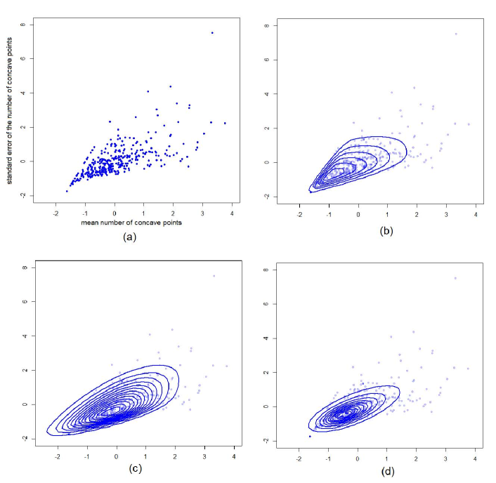
Figure 1: Modelling the WDBC data with three skew distributions. (a) A scatterplot of benign observations on the two variables: mean and standard error of the number of concave points. (b) The contours of the density of the fitted CFUSN distribution. (c) The contours of the density of the fitted restricted SN distribution. (d) The contours of the density of the fitted generalized hyperbolic distribution.

3 Mixture of CFUSS factor analyzers (CFUSSFA) model

Here, we propose to generalize the M$t$FA (20) model to the case where the factors and errors are jointly distributed as a CFUSS distribution. We replace the $t$-distribution in (27) with a CFUSS distribution. For simplicity, we focus on the class of SMCFUSN distributions. Let $\mbox{\boldmath$Y$}_{1},\ldots,\mbox{\boldmath$Y$}_{n}$ be a random sample of $n$ observations of $Y$. Accordingly, the mixture of SMCFUSN factor analzyers (SMCFUSNFA) can be formulated as

$$\mbox{\boldmath$Y$}_{j} = \mbox{\boldmath$\mu$}_{i}+\mbox{\boldmath$B$}_{i}\mbox{\boldmath$X$}_{ij}+\mbox{\boldmath$\epsilon$}_{ij},$$ (28)

with probability $\pi_{i}\;(i=1,\ldots,g)$, where

$$\left[\begin{array}[]{c}\mbox{\boldmath$X$}_{ij}\\ \mbox{\boldmath$\epsilon$}_{ij}\end{array}\right] \sim \mbox{{SMCFUSN}}_{q+p}\left(\left[\begin{array}[]{c}\mbox{\boldmath$0$}\\ \mbox{\boldmath$0$}\end{array}\right],\left[\begin{array}[]{cc}\mbox{\boldmath$I$}_{q}&\mbox{\boldmath$0$}\\ \mbox{\boldmath$0$}&\mbox{\boldmath$D$}_{i}\end{array}\right],\left[\begin{array}[]{c}\mbox{\boldmath$\Delta$}_{i}\\ \mbox{\boldmath$0$}\end{array}\right];F_{\mbox{\boldmath$\zeta$}_{i}}\right).$$ (37)

Some special cases of SMCFUSNFA shall be considered next.

3.1 The CFUSN factor analysis (CFUSNFA) model

The mixture of CFUSN factor analzyers (CFUSNFA) is a degenerate case of CFUSSFA. It can be formulated as

$$\mbox{\boldmath$Y$}_{j} = \mbox{\boldmath$\mu$}_{i}+\mbox{\boldmath$B$}_{i}\mbox{\boldmath$X$}_{ij}+\mbox{\boldmath$\epsilon$}_{ij},$$ (39)

with probability $\pi_{i}\;(i=1,\ldots,g)$, where

$$\left[\begin{array}[]{c}\mbox{\boldmath$X$}_{ij}\\ \mbox{\boldmath$\epsilon$}_{ij}\end{array}\right] \sim CFUSN_{q+p}\left(\left[\begin{array}[]{c}\mbox{\boldmath$0$}\\ \mbox{\boldmath$0$}\end{array}\right],\left[\begin{array}[]{cc}\mbox{\boldmath$I$}_{q}&\mbox{\boldmath$0$}\\ \mbox{\boldmath$0$}&\mbox{\boldmath$D$}_{i}\end{array}\right],\left[\begin{array}[]{c}\mbox{\boldmath$\Delta$}_{i}\\ \mbox{\boldmath$0$}\end{array}\right]\right).$$ (48)

Thus, marginally, the factors $\mbox{\boldmath$X$}_{ij}$ $(j=1,\ldots,n)$ follow a standard $q$-dimensional CFUSN distribution, whereas the errors $\mbox{\boldmath$\epsilon$}_{ij}$ follow a $p$-dimensional normal distribution. When $\mbox{\boldmath$\Delta$}=\mbox{\boldmath$0$}$, we retrieve the MFA model. When $r=1$, we retrieve a skew normal MFA model equivalent to the MSNFA model proposed by Lin et al. (2016). Note that in the formulation of the MSNFA model, the authors adopt a slightly different parametrization so that the factors have expected value being $\mathrm{𝟎}$ and the covariance matrix is equal to the identity matrix.

3.2 The CFUSH factor analysis (CFUSHFA) model

To obtain the mixture of CFUSH factor analzyers (CFUSHFA), let $F_{\mbox{\boldmath$\zeta$}_{i}}$ for the $i$th component denote the GIG distribution function with density defined in (6). Then $\mbox{\boldmath$\zeta$}_{i}$ contains the parameters $\psi_{i}$, $\chi_{i}$, and $\lambda_{i}$ for $i=1,\ldots,g$. The resulting model is a CFUSHFA model which is given by

$$\mbox{\boldmath$Y$}_{j} = \mbox{\boldmath$\mu$}_{i}+\mbox{\boldmath$B$}_{i}\mbox{\boldmath$X$}_{ij}+\mbox{\boldmath$\epsilon$}_{ij},$$ (49)

with probability $\pi_{i}\;(i=1,\ldots,g)$, where

$$\left[\begin{array}[]{c}\mbox{\boldmath$X$}_{ij}\\ \mbox{\boldmath$\epsilon$}_{ij}\end{array}\right] \sim \mbox{{CFUSH}}_{q+p}\left(\left[\begin{array}[]{c}\mbox{\boldmath$0$}\\ \mbox{\boldmath$0$}\end{array}\right],\left[\begin{array}[]{cc}\mbox{\boldmath$I$}_{q}&\mbox{\boldmath$0$}\\ \mbox{\boldmath$0$}&\mbox{\boldmath$D$}_{i}\end{array}\right],\left[\begin{array}[]{c}\mbox{\boldmath$\Delta$}_{i}\\ \mbox{\boldmath$0$}\end{array}\right],\psi_{i},\chi_{i},\lambda_{i}\right).$$ (58)

In this case, the marginal distribution of the factors $\mbox{\boldmath$X$}_{ij}$ is a standard $q$-dimensional CFUSH distribution, whereas the errors $\mbox{\boldmath$\epsilon$}_{ij}$ follow a $p$-dimensional hyperbolic distribution.

3.3 The CFUST factor analysis (CFUSTFA) model

Consider now adopting the CFUST distribution for the joint distribution of the factors and errors in (LABEL:SMCFUSNFA2). This corresponds to the special case of the SMCFUSNFA model with $F_{\mbox{\boldmath$\zeta$}_{i}}$ being the inverse gamma distribution function with parameter $\mbox{\boldmath$\zeta$}_{i}=\nu_{i}$. Henceforth, we shall refer to this model as the CFUST factor analysis (CFUSTFA) model. This model can be formulated as

$$\mbox{\boldmath$Y$}_{j} = \mbox{\boldmath$\mu$}_{i}+\mbox{\boldmath$B$}_{i}\mbox{\boldmath$X$}_{ij}+\mbox{\boldmath$\epsilon$}_{ij},$$ (60)

with probability $\pi_{i}\;(i=1,\ldots,g)$, where

$$\left[\begin{array}[]{c}\mbox{\boldmath$X$}_{ij}\\ \mbox{\boldmath$\epsilon$}_{ij}\end{array}\right] \sim CFUST_{q+p}\left(\left[\begin{array}[]{c}\mbox{\boldmath$0$}\\ \mbox{\boldmath$0$}\end{array}\right],\left[\begin{array}[]{cc}\mbox{\boldmath$I$}_{q}&\mbox{\boldmath$0$}\\ \mbox{\boldmath$0$}&\mbox{\boldmath$D$}_{i}\end{array}\right],\left[\begin{array}[]{c}\mbox{\boldmath$\Delta$}_{i}\\ \mbox{\boldmath$0$}\end{array}\right],\nu_{i}\right).$$ (69)

It is clear that, marginally, the factors $\mbox{\boldmath$X$}_{ij}$ $(j=1,\ldots,n)$ follow a standard $q$-dimensional CFUST distribution, whereas the errors $\mbox{\boldmath$\epsilon$}_{ij}$ follow a $p$-dimensional $t$-distribution. More specifically, $\mbox{\boldmath$X$}_{ij}\sim CFUST_{q}(\mbox{\boldmath$0$},\mbox{\boldmath$I$}_{q},\mbox{\boldmath$\Delta$}_{i},\nu_{i})$ and $\mbox{\boldmath$\epsilon$}_{ij}\sim t_{p}(\mbox{\boldmath$0$},\mbox{\boldmath$D$}_{i},\nu_{i})$. Note that similar to the $t$FA model, the $\mbox{\boldmath$X$}_{ij}$ and $\mbox{\boldmath$\epsilon$}_{ij}$ here are not independent but are uncorrelated. It follows from (60) that the mean and covariance matrix of the factors are given by

$$E\left(\mbox{\boldmath$X$}_{ij}\right)=a(\nu_{i})\mbox{\boldmath$\Delta$}_{i}\mbox{\boldmath$1$}_{r}$$

and

$$\mbox{cov}\left(\mbox{\boldmath$X$}_{ij}\right) = \left(\frac{\nu_{i}}{\nu_{i}-2}\right)\left[\mbox{\boldmath$I$}_{q}+\left(1-\frac{2}{\pi}\right)\mbox{\boldmath$\Delta$}_{i}\mbox{\boldmath$\Delta$}_{i}^{T}\right]+\left[\frac{2}{\pi}\left(\frac{2}{\nu_{i}-2}\right)-a(\nu_{i})^{2}\right]\mbox{\boldmath$\Delta$}_{i}\mbox{\boldmath$J$}_{r}\mbox{\boldmath$\Delta$}_{i}^{T},$$

respectively.

It follows from (60) that the marginal density of $\mbox{\boldmath$Y$}_{j}$ is a CFUST distribution; that is, given that $\mbox{\boldmath$Y$}_{j}$ belongs to the $i$th component of the mixture model, it is distributed as

$$\mbox{\boldmath$Y$}_{j} \sim \mbox{CFUST}_{p,r}(\mbox{\boldmath$\mu$}_{i},\mbox{\boldmath$B$}_{i}\mbox{\boldmath$B$}_{i}^{T}+\mbox{\boldmath$D$}_{i},\mbox{\boldmath$B$}_{i}\mbox{\boldmath$\Delta$}_{i},\nu_{i}).$$ (70)

Hence, the mean and covariance matrix of $\mbox{\boldmath$Y$}_{j}$ are given by

$$E(\mbox{\boldmath$Y$}_{j}) = \mbox{\boldmath$\mu$}+a(\nu_{i})\mbox{\boldmath$B$}_{i}\mbox{\boldmath$\Delta$}_{i}\mbox{\boldmath$1$}_{r},$$

and

$$\mbox{cov}(\mbox{\boldmath$Y$}_{j}) = \left(\frac{\nu_{i}}{\nu_{i}-2}\right)\left[\mbox{\boldmath$B$}_{i}\mbox{\boldmath$B$}_{i}^{T}+\mbox{\boldmath$D$}_{i}+\left(1-\frac{2}{\pi}\right)\mbox{\boldmath$B$}_{i}\mbox{\boldmath$\Delta$}_{i}\mbox{\boldmath$\Delta$}_{i}^{T}\mbox{\boldmath$B$}_{i}^{T}\right]$$ (71)

$$+\left[\frac{2}{\pi}\left(\frac{2}{\nu_{i}-2}\right)-a(\nu_{i})^{2}\right]\mbox{\boldmath$B$}_{i}\mbox{\boldmath$\Delta$}_{i}\mbox{\boldmath$J$}_{r}\mbox{\boldmath$\Delta$}_{i}^{T}\mbox{\boldmath$B$}_{i},$$

respectively.

Accordingly, the density of $\mbox{\boldmath$Y$}_{j}$ is a $g$-component CFUST mixture density, given by

$$f(\mbox{\boldmath$y$}_{j};\mbox{\boldmath$\Psi$}) = \sum_{i=1}^{g}\pi_{i}\,f_{\mbox{\tiny{CFUST}}}\left(\mbox{\boldmath$y$}_{j};\mbox{\boldmath$\mu$}_{i},\mbox{\boldmath$\Sigma$}_{i}^{*},\mbox{\boldmath$\Delta$}_{i}^{*},\nu_{i}\right),$$ (72)

where the vector $\mbox{\boldmath$\Psi$}=\left\{\pi_{1},\ldots,\pi_{g-1},\mbox{\boldmath$\theta$}_{1}^{T},\ldots,\mbox{\boldmath$\theta$}_{g}^{T}\right\}^{T}$ contains all the unknown parameters of the mixture model and $\mbox{\boldmath$\theta$}_{i}$ is the vector of unknown parameters of the $i$th component of the mixture model, comprising the elements of $\mbox{\boldmath$\mu$}_{i}$, $\mbox{\boldmath$\Delta$}_{i}$, $\mbox{\boldmath$B$}_{i}$, $\mbox{\boldmath$D$}_{i}$, and $\nu_{i}$. In the above, we let $\mbox{\boldmath$\Sigma$}^{*}=\mbox{\boldmath$B$}_{i}\mbox{\boldmath$B$}_{i}^{T}+\mbox{\boldmath$D$}$ and $\mbox{\boldmath$\Delta$}^{*}=\mbox{\boldmath$B$}_{i}\mbox{\boldmath$\Delta$}$ for notational convenience. It should be noted that $r$ need not be smaller than $q$. However, for simplicity, we will focus our attention on the cases where $r\leq q$ in the applications in Section 6. In addition, note that the CFUSTFA model reduces to the $t$FA model when $\mbox{\boldmath$\Delta$}_{i}=\mbox{\boldmath$0$}$, and reduces to the FA model when $\mbox{\boldmath$\Delta$}_{i}=\mbox{\boldmath$0$}$ and $\nu_{i}\rightarrow\infty$. Concerning identifiability, note that in the case of a CFUSTFA model $\mbox{\boldmath$X$}_{ij}$ is no longer rotational invariant due to its following a non-symmetrical distribution. Hence, the CFUSTFA model does not inherit the aforementioned issue concerning the $\mbox{\boldmath$B$}_{i}$ in the FA and $t$FA models.

4 Parameter estimation for the SMCFUSNFA model

Parameter estimation can be carried out using the maximum likelihood (ML) approach via the EM algorithm. For the CFUSSFA model, we exploit a variant of the EM algorithm that is useful when the M-step is relativity difficult to compute. The expectation–conditional maximization (ECM) algorithm (Meng and Rubin, 1993) replaces the M-step with a sequence of computationally simpler conditional–maximization (CM) steps by conditioning on the preceding parameters being estimated.

From (28) and (LABEL:SMCFUSNFA2) and using (3), the SMCFUSNFA model admits a five-level hierarchical representation. By expressing $\mbox{\boldmath$X$}_{ij}$ in terms of the latent variables $\mbox{\boldmath$U$}_{ij}$ and $W_{ij}$, it follows that

$$\mbox{\boldmath$Y$}_{j}\mid\mbox{\boldmath$x$}_{ij},w_{ij},Z_{ij}=1 \sim N_{p}\left(\mbox{\boldmath$B$}_{i}\mbox{\boldmath$x$}_{ij}+\mbox{\boldmath$\mu$}_{i},{w_{ij}}\mbox{\boldmath$D$}_{i}\right),$$

$$\mbox{\boldmath$X$}_{ij}\mid\mbox{\boldmath$u$}_{ij},w_{ij},Z_{ij}=1 \sim N_{q}\left(\mbox{\boldmath$\Delta$}_{i}|\mbox{\boldmath$u$}_{ij}|,{w_{ij}}\mbox{\boldmath$I$}_{q}\right),$$

$$|\mbox{\boldmath$U$}_{ij}|\mid w_{ij},Z_{ij}=1 \sim TN_{r}\left(\mbox{\boldmath$0$},{w_{ij}}\mbox{\boldmath$I$}_{r};\mathbb{R}^{+}\right),$$

$$W_{ij}\mid Z_{ij}=1 \sim F_{\mbox{\boldmath$\zeta$}_{i}},$$

$$\mbox{\boldmath$Z$}_{j} \sim \mbox{Multi}_{g}(1;\mbox{\boldmath$\pi$}),$$ (73)

where $\mbox{Multi}_{g}(1;\mbox{\boldmath$\pi$})$ denotes the multinomial distribution having $g$ categories with associated probabilities $\mbox{\boldmath$\pi$}=(\pi_{1},\ldots,\pi_{g})^{T}$. In the above, we let $\mbox{\boldmath$Z$}_{j}=(Z_{1j},\,\ldots,\,Z_{gj})^{T}$ $(j=1,\ldots,n)$ be the vector of latent indicator variables, where $Z_{ij}=1$ if $\mbox{\boldmath$y$}_{j}$ belongs to the $i$th component of the mixture model and $Z_{ij}=0$ otherwise. One may observe from (73) that the last four levels are identical to that for a finite mixture of SMCFUSN distributions.

Under the EM framework, the indicator labels $Z_{ij}$ and the latent variables $W_{ij}$, $\mbox{\boldmath$U$}_{ij}$, and $\mbox{\boldmath$X$}_{ij}$ are treated as missing data. Thus, the complete-data vector is given by $(\mbox{\boldmath$y$}^{T},\mbox{\boldmath$x$}^{T},\mbox{\boldmath$u$}^{T},\mbox{\boldmath$w$}^{T},\mbox{\boldmath$z$}^{T})^{T}$, where $\mbox{\boldmath$y$}=(\mbox{\boldmath$y$}_{1}^{T},\ldots,\mbox{\boldmath$y$}_{n}^{T})^{T}$, $\mbox{\boldmath$x$}=(\mbox{\boldmath$x$}_{11}^{T},\ldots,\mbox{\boldmath$x$}_{gn}^{T})^{T}$, $\mbox{\boldmath$u$}=(\mbox{\boldmath$u$}_{11}^{T},\ldots,\mbox{\boldmath$y$}_{gn}^{T})^{T}$, $\mbox{\boldmath$w$}=(w_{11}^{T},\ldots,w_{gn}^{T})^{T}$, and $\mbox{\boldmath$z$}=(\mbox{\boldmath$Z$}_{1}^{T},\ldots,\mbox{\boldmath$Z$}_{n}^{T})^{T}$. The log likelihood function and the $Q$-function can be derived using (73). Accordingly, the complete-data log likelihood function is given by

$$\log L_{c}(\mbox{\boldmath$\Psi$}) = \sum_{i=1}^{g}\sum_{j=1}^{n}Z_{ij}\left[\log\pi_{ij}-\frac{1}{2w_{ij}}\left(\mbox{\boldmath$x$}_{ij}-\mbox{\boldmath$\Delta$}_{i}|\mbox{\boldmath$u$}_{ij}|\right)^{T}\left(\mbox{\boldmath$x$}_{ij}-\mbox{\boldmath$\Delta$}_{i}|\mbox{\boldmath$u$}_{ij}|\right)+\log f_{\mbox{\boldmath$\zeta$}_{i}}(w_{ij})\right.$$ (74)

$$-\frac{1}{2w_{ij}}\left(\mbox{\boldmath$y$}_{j}-\mbox{\boldmath$\mu$}_{i}-\mbox{\boldmath$B$}_{i}\mbox{\boldmath$x$}_{ij}\right)^{T}\mbox{\boldmath$D$}_{i}^{-1}\left(\mbox{\boldmath$y$}_{j}-\mbox{\boldmath$\mu$}_{i}-\mbox{\boldmath$B$}_{i}\mbox{\boldmath$x$}_{ij}\right)-\frac{1}{2}\log|\mbox{\boldmath$D$}_{i}|\Big{]}$$

where additive constants and terms that do not involve any parameters of the model are omitted.

4.1 E-step

On the E-step, we compute the so-called $Q$-function, which is the conditional expectation of the complete-data log likelihood function given the observed data using the current estimates of the model parameters. Let the superscript $(k)$ on the parameters denote the updated estimates after the $k$th iteration of the EM algorithm. To compute the $Q$-function, we need to evaluate the following conditional expectations:

$$z_{ij}^{(k)} = E_{\Psi^{(k)}}\left[Z_{ij}=1\mid\mbox{\boldmath$y$}_{j}\right],$$ (75)

$$w_{ij}^{(k)} = E_{\Psi^{(k)}}\left[\frac{1}{W_{ij}}\mid\mbox{\boldmath$y$}_{j},Z_{ij}=1\right],$$ (76)

$$\mbox{\boldmath$e$}_{1ij}^{(k)} = E_{\Psi^{(k)}}\left[\frac{1}{W_{ij}}|\mbox{\boldmath$U$}_{ij}|\mid\mbox{\boldmath$y$}_{j},Z_{ij}=1\right],$$ (77)

$$\mbox{\boldmath$e$}_{2ij}^{(k)} = E_{\Psi^{(k)}}\left[\frac{1}{W_{ij}}|\mbox{\boldmath$U$}_{ij}||\mbox{\boldmath$U$}_{ij}|^{T}\mid\mbox{\boldmath$y$}_{j},Z_{ij}=1\right],$$ (78)

$$\mbox{\boldmath$e$}_{3ij}^{(k)} = E_{\Psi^{(k)}}\left[\frac{1}{W_{ij}}\mbox{\boldmath$X$}_{ij}\mid\mbox{\boldmath$y$}_{j},Z_{ij}=1\right],$$ (79)

$$\mbox{\boldmath$e$}_{4ij}^{{(k)}} = E_{\Psi^{(k)}}\left[\frac{1}{W_{ij}}\mbox{\boldmath$X$}_{ij}\mbox{\boldmath$X$}_{ij}^{T}\mid\mbox{\boldmath$y$}_{j},Z_{ij}=1\right],$$ (80)

$$\mbox{\boldmath$e$}_{5ij}^{(k)} = E_{\Psi^{(k)}}\left[\frac{1}{W_{ij}}\mbox{\boldmath$X$}_{ij}|\mbox{\boldmath$U$}_{ij}|^{T}\mid\mbox{\boldmath$y$}_{j},Z_{ij}=1\right].$$ (81)

The exact expressions for these conditional expectations will depend on the form of $F_{\mbox{\boldmath$\zeta$}}$. In addition, it should be noted that extra conditional expectations may be needed for the CM-steps related to the parameters in $\mbox{\boldmath$\zeta$}_{i}$. It is convenient to note that (75) to (78) are analogous to that for the corresponding SMCFUSN mixture model, except that the scale and skewness matrices are now given by $\mbox{\boldmath$\Sigma$}_{i}^{*}=\mbox{\boldmath$B$}_{i}\mbox{\boldmath$B$}_{i}^{T}+\mbox{\boldmath$D$}_{i}$ and $\mbox{\boldmath$\Delta$}_{i}^{*}=\mbox{\boldmath$B$}_{i}\mbox{\boldmath$\Delta$}_{i}$, respectively. In the case of a CFUSTFA model, for example, these are analogous to that for the FM-CFUST model which can be found in Lee and McLachlan (2016) and are also given in Appendix A for completeness.

The remaining conditional expectations can be derived by noting that the conditional distribution of $\mbox{\boldmath$X$}_{ij}$ given $\mbox{\boldmath$Y$}_{j}$, $\mbox{\boldmath$U$}_{ij}$, $w_{ij}$, and $Z_{ij}$ is a normal distribution. It can be shown that

$$\mbox{\boldmath$e$}_{3ij}^{(k)} = w_{ij}^{(k)}\mbox{\boldmath$C$}_{i}^{(k)}\mbox{\boldmath$B$}_{i}^{(k)^{T}}\mbox{\boldmath$D$}_{i}^{(k)^{-1}}\left(\mbox{\boldmath$y$}_{j}-\mbox{\boldmath$\mu$}_{i}^{(k)}\right)+\mbox{\boldmath$C$}_{i}^{(k)}\mbox{\boldmath$\Delta$}_{i}^{(k)}\mbox{\boldmath$e$}_{1ij}^{(k)},$$ (82)

$$\mbox{\boldmath$e$}_{5ij}^{(k)} = \mbox{\boldmath$C$}_{i}^{(k)}\mbox{\boldmath$B$}_{i}^{(k)^{T}}\mbox{\boldmath$D$}_{i}^{(k)^{-1}}\left(\mbox{\boldmath$y$}_{j}-\mbox{\boldmath$\mu$}_{i}^{(k)}\right)\mbox{\boldmath$e$}_{1ij}^{(k)^{T}}+\mbox{\boldmath$C$}_{i}^{(k)}\mbox{\boldmath$\Delta$}_{i}^{(k)}\mbox{\boldmath$e$}_{2ij}^{(k)},$$ (83)

$$\mbox{\boldmath$e$}_{4ij}^{{(k)}} = \mbox{\boldmath$e$}_{3ij}^{(k)}\left(\mbox{\boldmath$y$}_{j}-\mbox{\boldmath$\mu$}_{i}^{(k)}\right)^{T}\mbox{\boldmath$D$}_{i}^{(k)^{-1}}\mbox{\boldmath$B$}_{i}^{(k)}\mbox{\boldmath$C$}_{i}^{(k)^{T}}+\mbox{\boldmath$e$}_{5ij}^{(k)}\mbox{\boldmath$\Delta$}_{i}^{(k)^{T}}\mbox{\boldmath$C$}_{i}^{(k)^{T}}+\mbox{\boldmath$C$}_{i}^{(k)},$$ (84)

where $\mbox{\boldmath$C$}_{i}^{(k)^{-1}}=\mbox{\boldmath$B$}_{i}^{(k)^{T}}\mbox{\boldmath$D$}_{i}^{(k)^{-1}}\mbox{\boldmath$B$}_{i}^{(k)}+\mbox{\boldmath$I$}_{q}$.

4.2 CM-step

The CM-steps are implemented by calculating the updated estimates of the parameters in $\Psi$ by maximizing the $Q$-function obtained on the E-step. We proceed by updating the parameters in the order of $\pi_{i}$, $\mbox{\boldmath$\Delta$}_{i}$, $\mbox{\boldmath$B$}_{i}$, $\mbox{\boldmath$\mu$}_{i}$, and $\mbox{\boldmath$D$}_{i}$. More specifically, on the $(k+1)$th iteration of the ECM algorithm, the CM-steps are implemented as follows.

CM-step 1: Compute the updated estimate of $\pi_{i}$ using

$$\pi_{i}^{(k+1)} = \frac{1}{n}\sum_{j=1}^{n}z_{ij}^{(k)}.$$

CM-step 2: Compute the updated estimate of $\mbox{\boldmath$\Delta$}_{i}$ by maximising the $Q$-function over $\mbox{\boldmath$\Delta$}_{i}$, leading to

$$\mbox{\boldmath$\Delta$}_{i}^{(k+1)} = \left[\sum_{j=1}^{n}z_{ij}^{(k)}\mbox{\boldmath$e$}_{5ij}^{(k)}\right]\left[\sum_{j=1}^{n}z_{ij}^{(k)}\mbox{\boldmath$e$}_{2ij}^{(k)}\right]^{-1}.$$

CM-step 3: Fix $\mbox{\boldmath$\Delta$}_{i}=\mbox{\boldmath$\Delta$}_{i}^{(k)}$, then update $\mbox{\boldmath$B$}_{i}$ using

$$\mbox{\boldmath$B$}_{i}^{(k+1)} = \left[\sum_{j=1}^{n}z_{ij}^{(k)}\left(\mbox{\boldmath$y$}_{j}-\mbox{\boldmath$\mu$}_{i}^{(k+1)}\right)\mbox{\boldmath$e$}_{3ij}^{(k)^{T}}\right]\left[\sum_{j=1}^{n}z_{ij}^{(k)}\mbox{\boldmath$e$}_{4ij}^{(k)}\right]^{-1}.$$

CM-step 4: Fix $\mbox{\boldmath$\Delta$}_{i}=\mbox{\boldmath$\Delta$}_{i}^{(k)}$ and $\mbox{\boldmath$B$}_{i}=\mbox{\boldmath$B$}_{i}^{(k+1)}$. The location vector $\mbox{\boldmath$\mu$}_{i}$ can be updated by

$$\mbox{\boldmath$\mu$}_{i}^{(k+1)} = \frac{\sum_{j=1}^{n}z_{ij}^{(k)}w_{ij}^{(k)}\mbox{\boldmath$y$}_{j}-\mbox{\boldmath$B$}_{i}^{(k)}\mbox{\boldmath$\Delta$}_{i}^{(k)}\sum_{j=1}^{n}z_{ij}^{(k)}\mbox{\boldmath$e$}_{3ij}^{(k)}}{\sum_{j=1}^{n}z_{ij}^{(k)}w_{ij}^{(k)}}.$$

CM-step 5: Fix $\mbox{\boldmath$\Delta$}_{i}=\mbox{\boldmath$\Delta$}_{i}^{(k)}$ and $\mbox{\boldmath$\mu$}_{i}=\mbox{\boldmath$\mu$}_{i}^{(k+1)}$. The updated estimate of $\mbox{\boldmath$D$}_{i}$ can be obtained by maximizing the $Q$-function over $\mbox{\boldmath$d$}_{i}$, the vector containing the diagonal elements of $\mbox{\boldmath$D$}_{i}$. This leads to

$$\mbox{\boldmath$D$}_{i}^{(k+1)} = \mbox{diag}\left(\mbox{\boldmath$d$}_{i}^{(k+1)}\right),$$

where

$$\mbox{\boldmath$d$}_{i}^{(k+1)} = \mbox{diag}\left\{\sum_{j=1}^{n}z_{ij}^{(k)}\left[\mbox{\boldmath$B$}_{i}^{(k+1)}\mbox{\boldmath$e$}_{4ij}^{(k)}\mbox{\boldmath$B$}_{i}^{(k+1)^{T}}+w_{ij}^{(k)}\left(\mbox{\boldmath$y$}_{j}-\mbox{\boldmath$\mu$}_{i}^{(k+1)}\right)\left(\mbox{\boldmath$y$}_{j}-\mbox{\boldmath$\mu$}_{i}^{(k+1)}\right)^{T}\right.\right.$$

$$\left.\left.-\mbox{\boldmath$B$}_{i}^{(k+1)}\mbox{\boldmath$e$}_{3ij}^{(k)}\left(\mbox{\boldmath$y$}_{j}-\mbox{\boldmath$\mu$}_{i}^{(k+1)}\right)^{T}-\left(\mbox{\boldmath$y$}_{j}-\mbox{\boldmath$\mu$}_{i}^{(k+1)}\right)\mbox{\boldmath$e$}_{3ij}^{(k)^{T}}\mbox{\boldmath$B$}_{i}^{(k+1)^{T}}\right]\Bigg{\}}\right.\left[\sum_{j=1}^{n}z_{ij}^{(k)}\right]^{-1}.$$

CM-step 6: In the final CM-step, we compute the updated estimate of the parameters in $\mbox{\boldmath$\zeta$}_{i}$. Their expressions can be derived by maximizing the $Q$-function with respect to $\mbox{\boldmath$\zeta$}_{i}$. In the case of the CFUSTFA model, for example, $\mbox{\boldmath$\zeta$}_{i}$ contains only $\nu_{i}$. An updated estimate of $\nu_{i}$ is obtained by solving for $\nu_{i}$ the following equation,

$$0 = \left(\sum_{i=1}^{n}z_{ij}^{(k)}\right)\left[\log\left(\frac{\nu_{i}}{2}\right)-\psi\left(\frac{\nu_{i}}{2}\right)+1\right]$$

$$+\sum_{j=1}^{n}z_{ij}^{(k)}\left[\psi\left(\frac{\nu_{i}^{(k)}+p}{2}\right)-\log\left(\frac{\nu_{i}^{(k)}+\eta_{ij}^{(k+1)}}{2}\right)-\left(\frac{\nu_{i}^{(k)}+p}{\nu_{i}^{(k)}+\eta_{ij}^{(k+1)}}\right)\right],$$

where

$$\eta_{ij}^{(k+1)} = \left(\mbox{\boldmath$y$}_{j}-\mbox{\boldmath$\mu$}_{i}^{(k+1)}\right)^{T}\left(\mbox{\boldmath$B$}_{i}^{(k+1)}\mbox{\boldmath$\Omega$}_{i}^{(k+1)}\mbox{\boldmath$B$}_{i}^{(k+1)^{T}}+\mbox{\boldmath$D$}_{i}^{(k+1)}\right)^{-1}\left(\mbox{\boldmath$y$}_{j}-\mbox{\boldmath$\mu$}_{i}^{(k+1)}\right),$$

$$\mbox{\boldmath$\Omega$}_{i}^{(k+1)} = \mbox{\boldmath$I$}_{q}+\mbox{\boldmath$\Delta$}_{i}^{(k+1)}\mbox{\boldmath$\Delta$}_{i}^{(k+1)^{T}},$$

and where $\psi(\cdot)$ is the digamma function.

Given an initial value for the parameters in $\Psi$, the ECM algorithm alternates between the E and CM-steps until a specified convergence criterion is met. These will be detailed in the next section. Upon convergence, the predicted component memberships can be obtained by applying the maximum a posteriori (MAP) rule on the basis of the $z_{ij}^{(k)}$ (McLachlan and Peel, 2000); that is, $\mbox{\boldmath$y$}_{j}$ is assigned to the component to which it has the highest posterior probability of belonging. In addition, factor scores can be useful for subsequent analysis, for example, to visualise the data in a lower-dimensional latent subspace. For the SMCFUSNFA model, the estimated factor scores can be easily obtained using (79), and are given by

$$\hat{\mbox{\boldmath$u$}}_{j} = \sum_{i=1}^{g}z_{ij}^{(k)}\mbox{\boldmath$e$}_{3ij}^{(k)}.$$ (85)

5 Implementation

5.1 Starting Values

As the log likelihood function typically exhibits multiple local maxima, it is useful to try a variety of initial values using different starting strategies. An intuitive way to start the EM algorithm for the SMCFUSNFA model is to initialize the parameters according to the results of its nested model, for example, the corresponding restricted model with $r=1$, the symmetric version with $\mbox{\boldmath$\Delta$}=\mbox{\boldmath$0$}$, or the MFA model. In the latter case, as the MFA model does not account for skewness in the data, one may proceed by fitting a SMCFUSN distribution for the factor scores of each component of the MFA model and use the fitted parameters as the initial values.

Alternatively, a convenient way to generate valid initial values for the SMCFUSNFA model is to start from an initial clustering of the data given by, for example, $k$-means, random partitions, or other clustering methods. We then proceed to fit a FA model to each cluster to obtain an initial estimate of $\mbox{\boldmath$B$}_{i}$ and of $\mbox{\boldmath$D$}_{i}$. Then, for the skewness matrix, its initial values can be obtained by fitting a SMCFUSN distribution (or any of its nested skew distributions) to the factor scores of the FA model.

5.2 Convergence

We monitor the convergence of the ECM algorithm using Aitken’s acceleration criterion; see McLachlan and Krishnan (2008, p. 137). More specifically, the algorithm is stopped when the absolute difference between the log likelihood value and the asymptotic log likelihood is less than $\epsilon=10^{-6}$, that is, when

$$\log L_{\infty}-\log L^{(k)}<\epsilon,$$ (86)

where $L^{(k)}$ denotes the likelihood value after the $k$th iteration of the EM algorithm and $L_{\infty}$ denotes the asymptotic estimate of the log likelihood.

5.3 Model selection

In the ECM algorithm described above, the number of components $g$, the dimension of the latent factor subspace $q$, and the number of skewing variables $r$ are specified beforehand. In practice, these are typically unknown and need to be inferred from the data during model fitting. Usually, one proceeds by fitting the model for a range of values of $g$, $q$, and $r$ and to select an appropriate model from these candidates using some information criterion. The Bayesian information criterion (BIC) (Schwarz, 1978) is one of the more commonly used criteria, and is defined as

$$BIC = m\log(n)-2\log L(\hat{\mbox{\boldmath$\mbox{\boldmath$\Psi$}$}}),$$ (87)

where $m$ is the number of free parameters, $n$ is the number of observations, and $L(\hat{\mbox{\boldmath$\Psi$}})$ is the maximised likelihood value. In addition, we consider also the integrated completed likelihood (ICL) criterion (Biernacki et al., 2000) to assist in choosing a suitable model. By construction, the ICL aims at finding the number of clusters in the data whereas the BIC is aimed at determining the optimal number of components. The former is more conservative and carries a heavier penalty for more complex models. The ICL is defined as

$$ICL = BIC+2ENT,$$ (88)

where $ENT=-\sum_{i=1}^{g}\sum_{j=1}^{n}\hat{z}_{ij}\log(\hat{z}_{ij})$ is the estimated partition mean entropy. Thus ICL can be considered as a entropy-penalized version of BIC that penalizes the overlap between mixture components. For both BIC and ICL, a smaller value of the criterion is preferred.

6 Applications to real data

In this section, we illustrate the application of the SMCFUSNFA model in the particular case of the adoption of the CFUSTFA distribution. All analyses were performed in R (R Core Team, 2016). For comparison, we consider also the GHSTFA, CGHSTFA, and GHFA models, and the nested models of CFUSTFA, namely, MSNFA and MFA. The GHFA model is implemented in the R package MixGHD (Tortora et al., 2015). The GHSTFA, CGHSTFA, and MSNFA models are implemented as in Murray et al. (2014a), Murray et al. (2014b), and Lin et al. (2016), respectively. Initialization of model parameters and stopping rule are also implemented accordingly. Note that for the illustrations in this section, the number of components $g$ is assumed to be known for comparison purposes.

For the datasets considered in this section, the true group labels are available and hence we can assess the clustering performance of these models. Here we consider the correct classification rate (CCR), the Adjusted Rand Index (ARI), and the Adjusted Mutual Information (AMI). The CCR ranges from 0 to 1. It is calculated for all permutations of the cluster labels and the maximum CCR value across all permutations is reported. The ARI (Hubert and Arabie, 1985) is a variant of the Rand index (Rand, 1971) that corrects for chance so that it has a constant baseline equal to zero when the two clusterings are random and independent. An ARI of 1 indicating a perfect match to the ‘true’ labels. The Adjusted Mutual Information (AMI) (Vinh et al., 2010) is another popular measure used in the machine learning community. It is based on Shannon information theory whereas the ARI is based on pair-counting. Similar to ARI, the AMI is an adjusted version of the normalized mutual information that adjusts for chance. It has an expected value of zero for independent clusterings and takes the maximum value of one when the two clusterings are in perfect agreement.

6.1 The Hawks data

Our first illustration concerns a small dataset collected by researchers at the Cornell College in Iowa. The data consist of 19 variables taken from hawks at Lake MacBride. We consider here all the relevant continuous variables that have no missing observations. These are the length (mm) of primary wing feather, the weight (g) of the bird, the culmen length (mm), the hallux length (mm), and the tail length (mm). There are three species of hawks (Red-tailed, Sharp-shinned, and Copper’s) in the data and a total of 891 samples. A summary of the data (Table 3) indicates that hallux length exhibit strong asymmetry and kurtosis, although it may not be clear from Figure 2. Mild skewness and kurtosis were also observed for the other variables. From Figure 2, there seems to be only mild overlap between the three clusters and hence we can expect the models to perform reasonably well in this dataset. A closer inspection of the dataset suggests that skewness appears to be concentrated in a single direction (or very close to it) and hence the skew factor models that are formulated using skew distributions with a single skewing variable should not be disadvantaged.

Variable	minimum	sample mean	maximum	sample sd	sample skewness	sample kurtosis
Wing Length	37.2	315.9	480.0	95.3	-0.58	1.63
Weight	56.0	771.6	2030.0	462.9	-0.35	1.61
Culmen Length	8.6	21.8	39.2	7.3	-0.58	1.71
Hallux Length	9.5	26.4	341.4	17.8	11.36	184.52
Tail Length	119.0	198.9	288.0	36.8	-0.70	2.16

Table 3: An overview of the Hawks data.

Figure 2: Bivariate scatterplot of the Hawks dataset. Cooper’s hawks are represented by red dots, whereas red-tailed and sharp-shinned hawks are represented by blue and green dots, respectively.

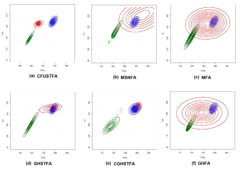
Figure 3: Contours of skew factor analyzers models fitted to the Hawks data. Results are shown on the variables Tail and Wing.

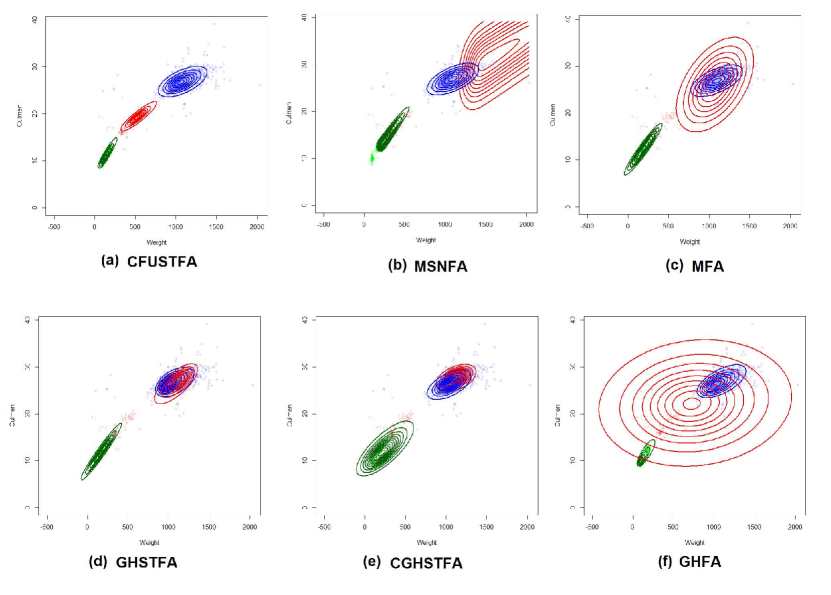
Figure 4: Contours of skew factor analyzers models fitted to the Hawks data. Results are shown on the variables Culmen and Weight.

Model	q	BIC	ICL	CCR	ARI	AMI
CFUSTFA	2	32832	32872	0.9237	0.8783	0.7506
MSNFA	1	33439	33469	0.88446	0.8045	0.6810
MFA	1	33846	33878	0.8867	0.8069	0.7063
GHSTFA	2	33457	33523	0.8945	0.8366	0.7189
CGHSTFA	3	34630	34774	0.9136	0.8416	0.6826
GHFA	2	33513	33486	0.8911	0.8267	0.7280

Table 4: Performance of skew factor models on the Hawks data.

We fitted the CFUSTFA model with a range of values of $q$ and $r$ such that its number of free parameters is less than that of a finite mixture of CFUST distribution with the corresponding value of $r$. We also fitted the GHSTFA, the CGHSTFA, and the GHFA models and also the nested models MSNFA and MFA with an appropriate range of values of $q$. Note that the range is dependent on the model. A summary of the preferred models by BIC is given in Table 4. However, it is noted that better clustering results can be achieved for the models with slightly higher values of BIC than that reported in Table 4.

In this example for the Hawks data, the CFUSTFA model preferred by BIC had $r=1$ and thus corresponds to a MSTFA model. It can be seen from Table 4 that the CFUSTFA obtained the highest CCR, ARI, and AMI. It is also preferred over the other models according to BIC and ICL. The MSNFA model is ranked second by BIC and ICL. The next two preferred models according to BIC and ICL are the GHSTFA and GHFA models, where the former is preferred over the latter by BIC and the opposite is preferred by ICL. According to Table 4, the GHSTFA model obtained slightly better clustering performance than the GHFA model according to CCR and ARI, although the AMI ranked the clustering results obtained by the GHFA model slightly more preferable than that of the GHSTFA model. We can also observe from Table 4 that the GHSTFA and CGHSTFA models have very similar performance. The CGHSTFA model gave slightly better clustering results in terms of the CCR and ARI than the GHSTFA model, but the latter model is not preferred to the CGHSTFA model in terms of BIC and ICL. This can be partly observed from Figures 3(d) and 3(e), where the CGHSTFA model appears to provide a closer fit to the data than the GHSTFA model. In particular, the location and shape of the component shown in red in Figures 3 and 4 are quite different.

On comparing the contours of the models in Figures 3 and 4, it can be observed that all of the considered models except the CFUSTFA model seem to have difficulty separating the two upper clusters (shown in red and blue). Overall, the visual impression from Figures 3 and 4 supports the preference by BIC and ICL which suggests that the CFUSTFA model provides a better fit relative to the other models considered in this dataset.

6.2 The melanoma data

We consider an application of mixtures of factor analyzers to the discrimination between benign and malignant melanoma from clinical and dermoscopic skin images. Images can be obtained from public databases such as ISIC (Codella et al., 2017); some examples are shown in Figure 5. Commonly used features for medical image processing were extracted from these images. These include some of those suggested by Ferris et al. (2015), such as eccentricity, equivalent diameter, perimeter, and solidity. For this illustration, 149 cases of benign lesions and 149 cases of malignant lesions were included – a total 298 images to be analyzed. We considered the fitting of the CFUSTFA, MSNFA, MFA, GHSTFA, CGHSTFA, and GHFA models to the data with $g=2$. The models were applied with $q$ varying from $1$ and $10$ (the maximum value of $q$ is dependent on the model). The best performing results are reported in Table 5. As can be observed from these results, this is a difficult dataset for clustering. The best clustering results are obtained by the CFUSTFA model which has an ARI of 0.57 and a CCR of 0.88. The next best performing model according to CCR and ARI is the GHFA model. However, its CCR is considerably lower (approximately 20% less) than that for the CFUSTFA model and its ARI is very low (ARI=0.11). The remaining models have similar performance to the GHSTFA model, which is the next best performing model according to CCR and ARI, as can be observed the results in Table 5. A cross-tabulation of the clustering results of the best performing models is given in Table 6. With the CFUSTFA model, there are 36 misclassified observations, whereas with the GHFA and GHSTFA models, there are 94 and 108 misclassified observations, respectively. In addition, it is of interest to note that the CFUSTFA model has only $q=3$ factors, whereas the other five models require more factors for this dataset (ranging from 7 to 10).

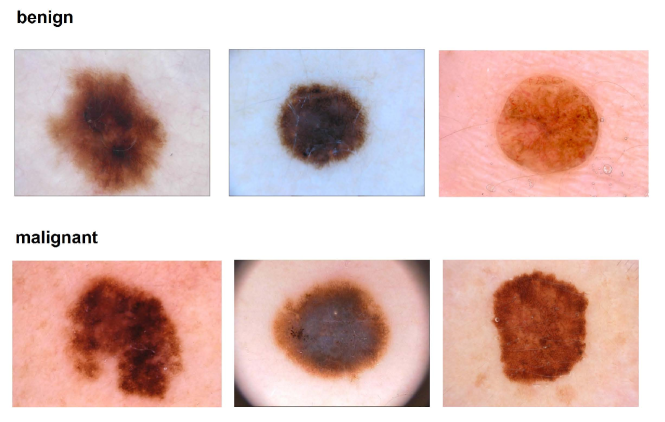
Figure 5: Example of benign and malignant images from the ISIC Archive.

Model	q	BIC	ICL	CCR	ARI	AMI
CFUSTFA	3	24193	24201	0.8792	0.5738	0.5007
MSNFA	10	22115	22125	0.6208	0.0560	0.0571
MFA	10	22253	22271	0.6376	0.0733	0.0718
GHSTFA	10	22092	22104	0.6376	0.0736	0.0827
CGHSTFA	8	25282	25331	0.6309	0.0670	0.1172
GHFA	7	28486	28465	0.6846	0.1336	0.1118

Table 5: Performance of skew factor models for the melanoma data.

	CFUSTFA		GHSTFA		GHFA
benign	144	5	137	12	126	23
malignant	31	118	96	53	71	78

Table 6: Cross-tabulation of clustering results of the CFUSTFA, GHSTFA, and GHFA models against the true group labels of the melanoma data.

7 Conclusions

This paper presents a novel generalization of the mixture of factor analyzers model based on a general skew distributional form that defines the class of SMCFUSN distributions. The proposed model provides a powerful tool for the flexible modelling of data exhibiting non-normal features including multimodality, skewness, and heavy-tailedness. For illustration, the focus has been on its special case, namely, the CFUST distribution. An ECM algorithm is derived for the mixture of SMCFUSN factor analzyers. Implementation issues such as strategies for generating starting values, the choice of convergence assessment, and model selection tools are also discussed. This class of mixture of skew factor analyzers formally embeds most of the existing skew factor analyzers, including the MSNFA, MSTFA, and CFUSSHFA models by Lin et al. (2016), Lin et al. (2018), and Murray et al. (2017c), respectively. An investigation of various existing mixtures of skew factor analyzers is presented, outlining the links and differences between them. Unlike existing models that are based on restricted skew distributions, the proposed SMCFUSNFA model has the capability of modelling multiple arbitrary directions of skewness at the same time. The usefulness of the SMCFUSNFA model is illustrated using the CFUSTFA model on some real datasets and its effectiveness over competing models is demonstrated in terms of various performance assessment measures.

Appendix A Expressions for the E-step of the ECM algorithm for the CFUSTFA model

For the CFUSTFA model, the E-step of the ECM algorithms involves four conditional expressions that are analogous to the case of mixtures of CFUST distributions. Technical details can be found in Lee and McLachlan (2016). The expressions for (75) to (78) are similar to that for (12), (13), (15), and (16), respectively, in Lee and McLachlan (2016). However, the scale matrices and skewness matrices in our case are given by $\mbox{\boldmath$\Sigma$}_{i}^{*^{(k)}}=\mbox{\boldmath$B$}_{i}^{(k)}\mbox{\boldmath$B$}_{i}^{(k)}+\mbox{\boldmath$D$}_{i}^{(k)}$ and $\mbox{\boldmath$\Delta$}_{i}^{*^{(k)}}=\mbox{\boldmath$B$}_{i}^{(k)}\mbox{\boldmath$\Delta$}_{i}^{(k)}$ $(i=1,\ldots,g)$, respectively. Thus, the expressions for the conditional expectations (75) to (78) are given by

$$z_{ij}^{(k)} = \frac{\pi_{i}^{(k)}f_{\mbox{\tiny{CFUST}}_{p,r}}(\mbox{\boldmath$y$}_{j};\mbox{\boldmath$\mu$}_{i}^{(k)},\mbox{\boldmath$\Sigma$}_{i}^{*^{(k)}},\mbox{\boldmath$\Delta$}_{i}^{*^{(k)}},\nu_{i}^{(k)})}{\sum_{i=1}^{g}\pi_{i}^{(k)}f_{\mbox{\tiny{CFUST}}_{p,r}}(\mbox{\boldmath$y$}_{j};\mbox{\boldmath$\mu$}_{i}^{(k)},\mbox{\boldmath$\Sigma$}_{i}^{*^{(k)}},\mbox{\boldmath$\Delta$}_{i}^{*^{(k)}},\nu_{i}^{(k)})},$$ (89)

$$w_{ij}^{(k)} = \left(\frac{\nu_{i}^{(k)}+p}{\nu_{i}^{(k)}+d_{ij}^{(k)}}\right)\frac{T_{r}\left(\mbox{\boldmath$c$}_{ij}^{(k)}\sqrt{\frac{\nu_{i}^{(k)}+p+2}{\nu_{i}+d_{ij}^{(k)}}};\mbox{\boldmath$0$},\mbox{\boldmath$\Lambda$}_{i}^{(k)},\nu_{i}^{(k)}+p+2\right)}{T_{r}\left(\mbox{\boldmath$c$}_{ij}^{(k)}\sqrt{\frac{\nu_{i}^{(k)}+p}{\nu_{i}+d_{ij}^{(k)}}};\mbox{\boldmath$0$},\mbox{\boldmath$\Lambda$}_{i}^{(k)},\nu_{i}^{(k)}+p\right)},$$ (90)

$$\mbox{\boldmath$e$}_{1ij}^{(k)} = w_{ij}^{(k)}E\left[\mbox{\boldmath$a$}_{ij}^{(k)}\right],$$ (91)

$$\mbox{\boldmath$e$}_{2ij}^{{(k)}} = w_{ij}^{(k)}E\left[\mbox{\boldmath$a$}_{ij}^{(k)}\mbox{\boldmath$a$}_{ij}^{(k)^{T}}\right],$$ (92)

where

$$d_{ij}^{(k)} = (\mbox{\boldmath$y$}_{j}-\mbox{\boldmath$\mu$}_{i}^{(k)})^{T}\mbox{\boldmath$\Omega$}_{i}^{(k)^{-1}}(\mbox{\boldmath$y$}_{i}-\mbox{\boldmath$\mu$}_{i}^{(k)}),$$

$$\mbox{\boldmath$c$}_{ij}^{(k)} = \mbox{\boldmath$\Delta$}_{i}^{*^{(k)^{T}}}\mbox{\boldmath$\Omega$}_{i}^{(k)^{-1}}(\mbox{\boldmath$y$}_{j}-\mbox{\boldmath$\mu$}_{i}^{(k)}),$$

$$\mbox{\boldmath$\Lambda$}_{i}^{(k)} = \mbox{\boldmath$I$}_{r}-\mbox{\boldmath$\Delta$}_{i}^{*^{(k)^{T}}}\mbox{\boldmath$\Omega$}_{i}^{(k)^{-1}}\mbox{\boldmath$\Delta$}_{i}^{(k)},$$

$$\mbox{\boldmath$\Omega$}_{i}^{(k)} = \mbox{\boldmath$\Sigma$}_{i}^{*^{(k)}}+\mbox{\boldmath$\Delta$}_{i}^{*^{(k)}}\mbox{\boldmath$\Delta$}_{i}^{*^{(k)^{T}}},$$

and where $\mbox{\boldmath$a$}_{ij}^{(k)}$ is a $r$-variate truncated $t$-random variable given by

$$\mbox{\boldmath$a$}_{ij}^{(k)} \sim Tt_{r}\left(\mbox{\boldmath$c$}_{ij}^{(k)},\left(\frac{\nu_{i}^{(k)}+d_{ij}^{(k)}}{\nu_{i}^{(k)}+p+2}\right)\mbox{\boldmath$\Lambda$}_{i}^{(k)},\nu_{i}^{(k)}+p+2;\mathbb{R}^{+}\right).$$

The last term in expressions (91) and (92) correspond to the first and second moment of $\mbox{\boldmath$a$}_{ij}^{(k)}$ and can be evaluated using formulae described in, for example, O’Hagan (1976), Ho et al. (2012), and in the appendix of Lee and McLachlan (2014).

References

- Arellano-Valle and Azzalini (2006) Arellano-Valle, R.B. and Azzalini, A. (2006). On the unification of families of skew-normal distributions. Scandinavian Journal of Statistics 33, 561–574.
- Arellano-Valle and Genton (2005) Arellano-Valle, R.B. and Genton, M.G. (2005). On fundamental skew distributions. Journal of Multivariate Analysis 96, 93–116.
- Azzalini and Capitanio (2014) Azzalini, A. and Capitanio, A. (2014). The Skew-Normal and Related Families. Cambridge: Cambridge University Press.
- Azzalini and Dalla Valle (1996) Azzalini, A. and Dalla Valle, A. (1996). The multivariate skew-normal distribution. Biometrika 83, 715–726.
- Biernacki et al. (2000) Biernacki, C., Celeux, G., and Govaert, G. (2000). Assessing a mixture model for clustering with the integrated completed likelihood. IEEE Transactions on Pattern Analysis and Machine Intelligence 22, 719–725.
- Browne and McNicholas (2015) Browne, R.P. and McNicholas, P.D. (2015). A mixture of generalized hyperbolic distributions. The Canadian Journal of Statistics 43, 176–198.
- Cabral et al. (2012) Cabral, C.R.B., Lachos, V.H., and Prates, M.O. (2012). Multivariate mixture modeling using skew-normal independent distributions. Computational Statistics and Data Analysis 56, 126–142.
- Codella et al. (2017) Codella, N., Gutman, D., Celebi, M.E., Helba, B., Marchetti, M.A., Dusza, S., Kalloo, A., Liopyris, K., Mishra, N., Kittler, H., and Halpern, A. (2017). Skin lesion analysis toward melanoma detection: A challenge at the 2017 International Symposium on Biomedical Imaging (ISBI), hosted by the International Skin Imaging Collaboration (ISIC). arXiv:1710.05006 .
- Dempster et al. (1977) Dempster, A.P., Laird, N.M., and Rubin, D.B. (1977). Maximum likelihood from incomplete data via the EM algorithm. Journal of Royal Statistical Society B 39, 1–38.
- Ferris et al. (2015) Ferris, L.K., Harkes, J.A., Gilbert, B., Winger, D.G., Golubets, K., Akilov, O., and Satyanarayanan, M. (2015). Computer-aided classification of melanocytic lesions using dermoscopic images. Journal of the American Academy of Dermatology 73, 769–776.
- Genton (2004) Genton, M.G. (Ed.). (2004). Skew-Elliptical Distributions and Their Applications: A Journey Beyond Normality. Boca Raton, Florida: Chapman & Hall, CRC.
- Ghahramani and Hinton (1997) Ghahramani, Z. and Hinton, G. (1997). The EM algorithm for factor analyzers. Technical Report No. CRG-TR-96-1 The University of Toronto: Toronto.
- Ho et al. (2012) Ho, H.J., Lin, T.I., Chen, H.Y., and Wang, W.L. (2012). Some results on the truncated multivariate distribution. Journal of Statistical Planning and Inference 142, 25–40.
- Hubert and Arabie (1985) Hubert, L. and Arabie, P. (1985). Comparing partitions. Journal of Classification 2, 193–218.
- Karlis and Santourian (2009) Karlis, D. and Santourian, A. (2009). Model-based clustering with non-elliptically contoured distributions. Statistics and Computing 19, 73–83.
- Kim et al. (2016) Kim, H.M., Maadooliat, M., Arellano-Valle, R.B., and Genton, M.G. (2016). Skewed factor models using selection mechanisms. Journal of Multivariate Analysis 145, 162–177.
- Kim (2016) Kim, S.G. (2016). An approximate fitting for mixture of multivariate skew normal distribution via EM algorithm. Korean Journal of Applied Statistics 29, 513–523.
- Lee and McLachlan (2014) Lee, S. and McLachlan, G.J. (2014). Finite mixtures of multivariate skew -distributions: Some recent and new results. Statistics and Computing 24, 181–202.
- Lee and McLachlan (2013) Lee, S.X. and McLachlan, G.J. (2013). On mixtures of skew-normal and skew -distributions. Advances in Data Analysis and Classification 7, 241–266.
- Lee and McLachlan (2016) Lee, S.X. and McLachlan, G.J. (2016). Finite mixtures of canonical fundamental skew -distributions: The unification of the restricted and unrestricted skew -mixture models. Statistics and Computing 26, 573–589.
- Lichman (2013) Lichman, M. (2013). UCI machine learning repository. URL http://archive.ics.uci.edu/ml.
- Lin (2009) Lin, T.I. (2009). Maximum likelihood estimation for multivariate skew normal mixture models. Journal of Multivariate Analysis 100, 257–265.
- Lin (2010) Lin, T.I. (2010). Robust mixture modeling using multivariate skew- distribution. Statistics and Computing 20, 343–356.
- Lin et al. (2016) Lin, T.I., McLachlan, G.J., and Lee, S.X. (2016). Extending mixtures of factor models using the restricted multivariate skew-normal distribution. Journal of Multivariate Analysis 143, 398–413.
- Lin et al. (2018) Lin, T.I., Wang, W.L., McLachlan, G.J., and Lee, S.X. (2018). Robust mixtures of factor analysis models using the restricted multivariate skew- distribution. Statistical Modelling 18, 50–72.
- Lin et al. (2015) Lin, T.I., Wu, P.H., McLachlan, G.J., and Lee, S.X. (2015). A robust factor analysis model using the restricted skew -distribution. TEST 24, 510–531.
- Maleki et al. (2018) Maleki, M., Wraith, D., and Arellano-Valle, R.B. (2018). Robust finite mixture modeling of multivariate unrestricted skew-normal generalized hyperbolic distributions. Statistics and Computing .
- Maruotti et al. (2017) Maruotti, A., Bulla, J., Lagona, F., Picone, M., and Martella, F. (2017). Dynamic mixtures of factor analyzers to characterize multivariate air pollutant exposures. Annals of Applied Statistics 3, 1617–1648.
- McLachlan et al. (2007) McLachlan, G.J., Bean, R.W., and Jones, B.T. (2007). Extension of the mixture of factor analyzers model to incorporate the multivariate -distribution. Computational Statistics and Data Analysis 51, 5327––5338.
- McLachlan and Krishnan (2008) McLachlan, G.J. and Krishnan, T. (2008). (Second Edition). The EM Algorithm and Extensions. Hoboken, New Jersey: Wiley.
- McLachlan and Lee (2016) McLachlan, G.J. and Lee, S.X. (2016). Comment on “On nomenclature for, and the relative merits of, two formulations of skew distributions” by A. Azzalini, R. Browne, M. Genton, and P. McNicholas. Statistics and Probability Letters 116, 1–5.
- McLachlan and Peel (2000) McLachlan, G.J. and Peel, D. (2000). Finite Mixture Models. New York: Wiley.
- McLachlan et al. (2003) McLachlan, G.J., Peel, D., and Bean, R.W. (2003). Modelling high-dimensional data by mixtures of factor analyzers. Computational Statistics and Data Analysis 41, 379–388.
- Meng and Rubin (1993) Meng, X. and Rubin, D. (1993). Maximum likelihood estimation via the ECM algorithm: a general framework. Biometrika 80, 267–278.
- Montanari and Viroli (2010) Montanari, A. and Viroli, C. (2010). A skew-normal factor model for the analysis of student satisfaction towards university courses. Journal of Applied Statistics 37, 463–487.
- Murray et al. (2014a) Murray, P., Browne, R., and McNicholas, P. (2014a). Mixtures of skew- factor analyzers. Computational Statistics and Data Analysis 77, 326–335.
- Murray et al. (2014b) Murray, P., McNicholas, P., and Browne, R. (2014b). Mixtures of common skew- factor analyzers. Stat 3, 68–82.
- Murray et al. (2017a) Murray, P.M., Browne, R.P., and McNicholas, P.D. (2017a). Hidden truncation hyperbolic distributions, finite mixtures thereof, and their application for clustering. Journal of Multivariate Analysis 161, 141–156.
- Murray et al. (2017b) Murray, P.M., Browne, R.P., and McNicholas, P.D. (2017b). A mixture of SDB skew- factor analyzers. Econometrics and Statistics 3, 160–168.
- Murray et al. (2017c) Murray, P.M., Browne, R.P., and McNicholas, P.D. (2017c). Mixtures of hidden truncation hyperbolic factor analyzers. arXiv:1711.01504 .
- O’Hagan (1976) O’Hagan, A. (1976). Moments of the truncated multivariate- distribution. http://www.tonyohagan.co.uk/academic/pdf/trunc\_multi\_t.PDF.
- Pyne et al. (2009) Pyne, S., Hu, X., Wang, K., Rossin, E., Lin, T.I., Maier, L.M., Baecher-Allan, C., McLachlan, G.J., Tamayo, P., Hafler, D.A., De Jager, P.L., and Mesirow, J.P. (2009). Automated high-dimensional flow cytometric data analysis. Proceedings of the National Academy of Sciences USA 106, 8519–8524.
- R Core Team (2016) R Core Team (2016). R: A Language and Environment for Statistical Computing. URL http://www.R-project.org/. R Foundation for Statistical Computing, Vienna, Austria. ISBN 3-900051-07-0.
- Rand (1971) Rand, W.M. (1971). Objective criteria for the evaluation of clustering methods. Journal of the American Statistical Association 66, 846–850.
- Sahu et al. (2003) Sahu, S.K., Dey, D.K., and Branco, M.D. (2003). A new class of multivariate skew distributions with applications to Bayesian regression models. The Canadian Journal of Statistics 31, 129–150.
- Schwarz (1978) Schwarz, G. (1978). Estimating the dimension of a model. Annals of Statistics 6, 461–464.
- Seshadri (1997) Seshadri, V. (1997). Halphen’s laws. In Encyclopedia of Statistical Sciences, S. Kotz, C. B. Read, and D. L. Banks (Eds.). New York: Wiley, pp. 302–306.
- Tortora et al. (2015) Tortora, C., Browne, R.P., Franczak, B.C., and McNicholas, P.D. (2015). MixGHD: Model Based Clustering, Classification and Discriminant Analysis Using the Mixture of Generalized Hyperbolic Distributions. URL http://cran.r-project.org/web/packages/MixGHD. R package version 1.7.
- Tortora et al. (2016) Tortora, C., McNicholas, P., and Browne, R. (2016). A mixture of generalized hyperbolic factor analyzers. Advances in Data Analysis and Classification 10, 423–440.
- Vinh et al. (2010) Vinh, N.X., Epps, J., and Bailey, J. (2010). Information theoretic measures for clusterings comparison: Variants, properties, normalization and correction for chance. Journal of Machine Learning Research 11, 2227–2240.
- Wall et al. (2012) Wall, M.M., Guo, J., and Amemiya, Y. (2012). Mixture factor analysis for approximating a non-normally distributed continuous latent factor with continuous and dichotomous observed variables. Multivariate Behavioral Research 47, 276–313.
- Yamamoto et al. (2005) Yamamoto, H., Nankaku, Y., Miyajima, C., Tokuda, K., and Kitamura, T. (2005). Parameter sharing in mixture of factor analyzers for speaker identification. IEICE Transactions on Information and Systems 88, 418–424.
- Zhoe and Mobasher (2006) Zhoe, Y.K. and Mobasher, B. (2006). Web user segmentation based on a mixture of factor analyzers. Lecture Notes in Computer Science 4082, 11–20.