Explaining a changeover from normal to super diffusion in time-dependent billiards

Abstract

The changeover from normal to super diffusion in time dependent billiards is explained analytically. The unlimited energy growth for an ensemble of bouncing particles in time dependent billiards is obtained by means of a two dimensional mapping of the first and second moments of the velocity distribution function. We prove that for low initial velocities the mean velocity of the ensemble grows with exponent $\sim 1/2$ of the number of collisions with the border, therefore exhibiting normal diffusion. Eventually, this regime changes to a faster growth characterized by an exponent $\sim 1$ corresponding to super diffusion. For larger initial velocities, the temporary symmetry in the diffusion of velocities explains an initial plateau of the average velocity.

As coined by Enrico Fermi Ref1 Fermi acceleration (FA) is a phenomenon where an ensemble of classical and non interacting particles acquires energy from repeated elastic collisions with a rigid and time varying boundary. It is typically observed in billiards Ref2 ; Ref3 ; Ref4 whose boundaries are moving in time Ref5 ; Ref6 ; Ref7 ; Ref7b ; Ref7c . If the motion of the boundary is random and the initial velocity is small enough Ref8 , the growth of the average velocity is proportional to $n^{1/2},$ with $n$ denoting the number of collisions. If the initial velocity is larger, a plateau of constant velocity is observed in a plot ${\overline{V}}~{}vs.~{}n$ which is explained from the symmetry of the velocity diffusion Ref9 . The symmetry warrants that part of the ensemble grows and part of it decreases in such a way the growing parcel cancels the portion decreasing. As soon as such symmetry is broken the constant regime is changed to a regime of growth. For deterministic oscillations of the border, the scenario is different. Breathing oscillations preserve the shape but not the area of the billiard. It is known that the average velocity evolves in a sub-diffusive manner with a slope of the order of $1/6$ Ref10 ; Ref11 . For oscillations preserving the area but not the shape of the billiard there are two regimes of growth. For short time the diffusion of velocities is normal passing to super diffusion regime for large enough number of collisions Ref11b . This changeover is, so far, not yet explained and our contribution in this letter is to fill up this gap in the theory. This is achieved by studying the momenta of the velocity distribution function, noticing that the dynamical angular/time variables have an inhomogeneous distribution in phase space.

The results presented in this letter are illustrated by a time-dependent oval-billiard Ref12 whose phase space is mixed when the boundary is static. The boundary of the billiard is written as $R_{b}(\theta,t)=1+\epsilon\left[1+a\cos(t)\right]\cos(p\theta)$ where $R_{b}$ is the radius of the boundary in polar coordinates, $\theta$ is the polar angle, $\epsilon$ controls the circle deformation, $p>0$ is an integer number Ref13 given the shape of the boundary, $t$ is the time and $a$ is the amplitude of oscillation of the boundary. Figure 1 shows a typical scenario of the boundary and three collisions illustrating the dynamics.

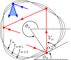
Figure 1: (Color online) Three consecutive collisions of a particle in a deterministic time time dependent billiard (red trajectory). Illustration of the reflection angle range for a billiard with random motion in the boundary (blue). The relevant angles and velocity are shown for the $n$th collision.

Figure 2: (Color online) Plot of $\overline{V}~{}vs.~{}n$ for different initial velocities, as labeled in the figure. Three different regimes are clear in the figure. For large initial velocities, a constant plateau dominates the dynamics for short $n$. After a first crossover, the average velocity starts to grow as a power law diffusing the velocity as a normal diffusion with slope of $0.481(9)$. Soon after, there is a second crossover where the normal diffusion is replaced by a super diffusion with slope $0.962(6)$. The right panels show portions of a single realization in the $(V,t)$-space where $A$ identifies normal diffusion and $B$ super diffusion. The parameters used are $\epsilon=0.08$, $a=0.5$ and $p=3$.

The dynamics of the particle is given in terms of a discrete, nonlinear and four dimensional mapping of the type $A:R^{4}\rightarrow R^{4}$ that transforms the dynamical variables at collision $n$ to their new values at collision $n+1$, $(\theta_{n+1},\alpha_{n+1},V_{n+1},t_{n+1})=A(\theta_{n},\alpha_{n},V_{n},t_{n})$ where $V_{n}=|\vec{V}_{n}|$ denotes the magnitude of the velocity particle after collision $n$, and $\alpha_{n}$ corresponds the angle between the particle trajectory and the tangent line at the $n^{th}$ collision with the boundary at the polar angle $\theta_{n}$ and collision time $t_{n}$ (see fig. 1). Given that each particle moves along a straight line between collisions and with constant speed, the radial position of the particle is given by $R_{p}(t)=\sqrt{X^{2}(t)+Y^{2}(t)}$, where $X(t)$ and $Y(t)$ are the rectangular coordinates of the particle at the time $t$. The angular position $\theta_{n+1}$ is obtained by the numerical solution of $R_{p}(\theta_{n+1},t_{n+1})=R_{b}(\theta_{n+1},t_{n+1})$. The time at collision $n+1$ is given by $t_{n+1}=t_{n}+{{\sqrt{\Delta X^{2}+\Delta Y^{2}}}\over|\vec{V_{n}}|}$, where $\Delta X=X_{p}(\theta_{n+1},t_{n+1})-X(\theta_{n},t_{n})$ and $\Delta Y=Y_{p}(\theta_{n+1},t_{n+1})-Y(\theta_{n},t_{n})$. Because the referential frame of the boundary is non inertial, a change of referential must be made before the application of the momentum conservation law. The reflection laws at the instant of collision are $\vec{V^{\prime}}_{n+1}\cdot\vec{T}_{n+1}=\xi\vec{V^{\prime}}_{n}\cdot\vec{T}_{n+1},$ and $\vec{V^{\prime}}_{n+1}\cdot\vec{N}_{n+1}=-\kappa\vec{V^{\prime}}_{n}\cdot\vec{N}_{n+1}$, where the unit tangent and normal vectors are $\vec{T}_{n+1}=\cos(\phi_{n+1})\hat{i}+\sin(\phi_{n+1})\hat{j}$, $\vec{N}_{n+1}=-\sin(\phi_{n+1})\hat{i}+\cos(\phi_{n+1})\hat{j}$ and $\xi,\kappa\in[0,1]$ are the restitution coefficients for the tangent and normal directions. The term $\vec{V^{\prime}}$ corresponds the velocity of the particle measured in the non-inertial reference frame. The tangential and normal components of the velocity after collision $n+1$ are

$$\vec{V}_{n+1}\cdot\vec{T}_{n+1} = \xi\vec{V}_{n}\cdot\vec{T}_{n+1}+(1-\xi)\vec{V}_{b}\cdot\vec{T}_{n+1},$$ (1)

$$\vec{V}_{n+1}\cdot\vec{N}_{n+1} = -\kappa\vec{V}_{n}\cdot\vec{N}_{n+1}+(1+\kappa)\vec{V}_{b}\cdot\vec{N}_{n+1},$$ (2)

where $\vec{V}_{b}(t_{n+1})={dR_{b}(t)\over{dt}}\Big{|}_{t_{n+1}}[\cos(\theta_{n+1})\widehat{i}+\sin(\theta_{n+1})\widehat{j}]$ is the velocity of the moving boundary at time $t_{n+1}$. The velocity of the particle after the collision $n+1$ is given by ${V}_{n+1}=\sqrt{(\vec{V}_{n+1}\cdot\vec{T}_{n+1})^{2}+(\vec{V}_{n+1}\cdot\vec{N}_{n+1})^{2}}$, while the angle $\alpha_{n+1}$ is written as $\alpha_{n+1}=\arctan\left[{\vec{V}_{n+1}\cdot\vec{N}_{n+1}\over\vec{V}_{n+1}\cdot\vec{T}_{n+1}}\right]$.

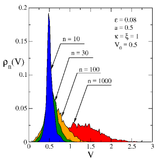
Figure 3: (Color online) Plot of the evolution of the velocity distribution function $\rho_{n}(V)$ for an ensemble of $5000$ particles after different number of collisions. The parameters used are $\epsilon=0.08$, $a=0.5$ and $p=3$.

Given an initial condition $(\theta_{n},\alpha_{n},V_{n},t_{n})$, the dynamical properties of the system can be obtained through application of the previous equations. We are interested in the behavior of the average velocity, obtained from two different kinds of average, namely $\overline{V}_{n}={1\over M}\sum_{i=1}^{M}{1\over{n+1}}\sum_{j=0}^{n}|\vec{V}|_{i,j},$ where the first summation is made over an ensemble of different initial conditions randomly distributed in $t\in[0,2\pi]$, $\alpha\in[0,\pi]$ and $\theta\in[0,2\pi]$ for a fixed initial velocity while the second summation corresponds to an average made over the orbit, hence in time. We considered $M=5000$ and $n=10^{7}$ collisions. Figure 2 shows the behavior of $\overline{V}~{}vs.~{}n$ for different initial velocities. Three different kinds of behavior can be seem from the figure. If the initial velocity is large, the curve of average velocity exhibits a constant plateau. The size of the plateau depends on the value of the initial velocity (see Ref. Ref9 for a discussion of such kind of behavior in a two dimensional mapping). A higher initial velocity, leads to a longer plateau. A first crossover is observed changing the behavior of the constant regime to the regime of growth with a slope of growth typical of normal diffusion. A numerical fitting gives a slope $0.481(9)$. The regime of normal diffusion then reaches a second crossover passing to a faster regime of growth named as super diffusion with slope $0.962(6)$. The panels on the right hand side of fig. 2, give the plot of a single realization in the $(V,t)$-space where $A$ corresponds to normal diffusion and $B$ to super diffusion. We emphasize when the perturbation on the boundary is random, the dynamics in the $(V,t)$-space is similar to what is observed in $A$ with a constant slope of growth about $1/2$ therefore characterized by normal diffusion. When the restitution coefficients $\xi,\kappa\neq 1$, inelastic collisions occur leading to a different scenario Ref14 , where the energy growth is interrupted by the violation of Liouville’s theorem and attractors emerge in the phase space.

The explanation of the initial plateau is related to the behavior of the velocity distribution function Ref14 . For an initial velocity larger than the maximum moving wall velocity, say $V_{max}=a\epsilon$, the following is observed: (1) Part of the ensemble of particles acquires energy leading to such portion of the ensemble to grow energy; (2) However, another part of the ensemble leads to decreasing of velocity. Each parcel cancels each other producing the constant plateau. The decrease however is limited to the lower bound of the velocity, in this case, null velocity. When the particles reach the velocity lower bound, the symmetry of the velocity diffusion is broken leading to a crossover between the constant regime and the growth regime. Figure 3 shows the evolution of the velocity distribution function $\rho_{n}(V)$, for an ensemble of particles as the number of collisions is increased.

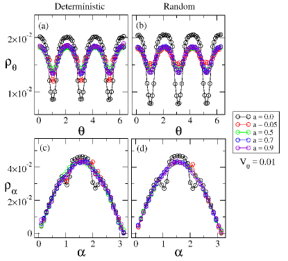
Figure 4: (Color online) Plot of the numerical distribution functions $\rho_{\theta}(\theta)=\int\tilde{F}(\theta,\alpha)d\alpha$ and $\rho_{\alpha}(\alpha)=\int\tilde{F}(\theta,\alpha)d\theta$ for deterministic and non-deterministic (random) billiards at various amplitude of oscillations. The parameters used are $\epsilon=0.08$, $a=0.5$ and $p=3$.

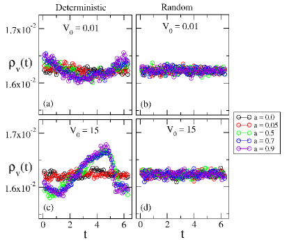
Figure 5: Plot of the numerical collision time distribution functions $\rho_{V}(t)$ for deterministic and non-deterministic (random) billiards at various amplitude of oscillations and two different initial velocities, as shown in the figure. The parameters used are $\epsilon=0.08$, $a=0.5$ and $p=3$.

The velocity of a particle after collision with the wall $\tilde{V}$, can be written in the form

$$\tilde{V}(\alpha,\theta,t,V)=V+\zeta(\alpha,\theta,t,V),$$ (3)

where $V$ is the velocity just before the collision. From this, the mean velocity of an ensemble of particles just after the $n^{th}$ collision takes the form

$$\overline{V}_{n+1}=\overline{V}_{n}+\delta\overline{V}_{n},$$ (4)

where

$$\overline{V}_{n} =\int_{0}^{\infty}\!\!\int_{0}^{2\pi}\!\!\int_{0}^{2\pi}\!\!\int_{0}^{\pi} V\mathcal{F}_{n}(\alpha,\theta,t,V)d\alpha d\theta dtdV,$$ (5)

$$\delta\overline{V}_{n} =\int_{0}^{\infty}\!\!\int_{0}^{2\pi}\!\!\int_{0}^{2\pi}\!\!\int_{0}^{\pi} \zeta(\alpha,\theta,t,V)\mathcal{F}_{n}(\alpha,\theta,t,V)\times$$ (6)

$$d\alpha d\theta dtdV,$$

and $\mathcal{F}_{n}(\alpha,\theta,t,V)$, is the phase space distribution function just before collision $n$. In the case of interest the distribution function can be factored in the form

$$\mathcal{F}_{n}(\alpha,\theta,t,V)=F(\theta,\alpha)\rho_{V}(t)\rho_{n}(V),$$ (7)

where $F(\alpha,\theta)$ is the $\alpha-\theta$ distribution, $\rho_{V}(t)$ is the collision time distribution and $\rho_{n}(V)$ is the velocity distribution function. The $F(\alpha,\theta)$ distribution is mainly determined by the billiard geometry and is only weakly modified by the wall oscillation, consequently it can be regarded as independent of the index $n$, the collision time distribution $\rho_{V}(t)$ depends on the velocity but not on the index $n$ and the velocity distribution function $\rho_{n}(V)$ depends on both the velocity and the index. To understand the evolution of the mean velocity of the ensemble we do not require to determine the evolution of the global distribution function. Inserting eq. (7) in eq. (5), and defining the partial mean

$$U(V) =\int_{0}^{2\pi}\!\!\int_{0}^{2\pi}\!\!\int_{0}^{\pi} \zeta(\alpha,\theta,t,V)F(\theta,\alpha)\rho_{V}(t)d\alpha d\theta dt,\quad$$ (8)

we obtain a compact expression for the change in the mean velocity

$$\delta\overline{V}_{n} =\int_{0}^{\infty} \rho_{n}(V)U(V)dV,$$ (9)

where the partial mean $U(V)$ can be expanded around the mean velocity $\overline{V}_{n}$

$$U(V)\approx U(\overline{V}_{n})+U^{\prime}(\overline{V}_{n})(V-\overline{V}_{n})+{1\over{2}}U^{\prime\prime}(\overline{V}_{n})(V-\overline{V}_{n})^{2}+...$$ (10)

This approximation becomes poor as we move far from the distribution mean. However, the velocity distribution $\rho_{n}(V)$ drops for large and small values of $V$, and the integrand in eq. (9) vanishes where the Taylor expansion is not accurate. Inserting eq. (10) in eq. (9) and replacing in eq. (4) we obtain a second order approximation of the $n+1$ mean velocity

$$\overline{V}_{n+1}=\overline{V}_{n}+U(\overline{V}_{n})+{1\over 2}U^{\prime\prime}(\overline{V}_{n})(\overline{V^{2}_{n}}-\overline{V_{n}}^{2}),$$ (11)

which depends on the quadratic mean of the velocity at collision $n$. An equation for the evolution of the quadratic mean is also needed. For the quadratic velocity after collision $\tilde{V}^{2}$, the collision rule can be also written in the form

$$\tilde{V}^{2}(\alpha,\theta,t,V)=V^{2}+\psi(\alpha,\theta,t,V),$$ (12)

where $V$ is again the velocity before collision. Reproducing the same arguments used for the mean velocity we obtain

$$\overline{V^{2}}_{n+1}=\overline{V^{2}}_{n}+W(\overline{V}_{n})+{1\over 2}W^{\prime\prime}(\overline{V}_{n})(\overline{V^{2}_{n}}-\overline{V_{n}}^{2}),$$ (13)

where

$$W(V)\!\! =\int_{0}^{2\pi}\!\!\int_{0}^{2\pi}\!\!\int_{0}^{\pi} \!\!\psi(\alpha,\theta,t,V)F(\theta,\alpha)\rho_{V}(t)d\alpha d\theta dt.\qquad$$ (14)

As will be shown later the inhomogeneous nature of $F(\theta,\alpha)$ is a fundamental aspect of super diffusion. It can be related to the presence of low period saddles in the static billiard Ref15 , where the collisions occur more often Ref16 , leading to an increase in the distribution value. Figure 4 we show line-integrated profiles of $F(\alpha,\theta)$ for both deterministic and random oscillations of the billiard boundary.

In the limit of high velocities or small amplitudes of the wall motion it can be shown that $\zeta(\alpha,\theta,t,V)\approx{\psi(\alpha,\theta,t,V)}/{2V},$ which leads to

$$U(V)\approx{W(V)}/{2V}.$$ (15)

This results in an approximated form for the two-dimensional mapping of the velocity mean and the quadratic velocity mean are

$$\overline{V}_{n+1} = \overline{V}_{n}+{1\over 2}{W_{n}}{\overline{V^{2}_{n}}}/{\overline{V_{n}}^{3}}+{1\over 2}\left({1\over 2}\overline{V_{n}}W^{\prime\prime}_{n}-W^{\prime}_{n}\right)$$

$$\times\left({\overline{V_{n}^{2}}}/{\overline{V_{n}}^{2}}-1\right),$$

$$\overline{V^{2}}_{n+1} = \overline{V^{2}}_{n}+W_{n}+{1\over 2}W^{\prime\prime}_{n}(\overline{V^{2}_{n}}-\overline{V_{n}}^{2}),$$ (16)

where $W_{n}=W(\overline{V_{n}}),W^{\prime}_{n}=W^{\prime}(\overline{V_{n}})$ and $W^{\prime\prime}_{n}=W^{\prime\prime}(\overline{V_{n}})$. This mapping is general and its its behavior depends on the particular form of the function $W(V)$ for the system under consideration. For instance, for the time-dependent oval billiard one can show

$$\psi(\alpha,\theta,t) = 4(a\epsilon)^{2}\cos^{2}(p\theta)\sin^{2}(t)+$$

$$-4a\epsilon V\cos(p\theta)\sin(\alpha)\sin(t),$$

and the collision time distribution can be approximated by (see fig. 5(a,c))

$$\rho_{V}(t)={1\over 2\pi}\left[1-a\epsilon\chi(V)\sin(t)\right],$$ (18)

where $\chi(V)$ is a slowly changing function of $V$ that vanishes for $V=0$ and saturates at $\chi^{*}$ for large $V$. This distribution develops due to the correlation between subsequent collisions for higher velocities for which the time between collisions is small compared to the wall oscillation period. Expectedly, the harmonic part is removed when the wall oscillations are random (see fig. 5(b,d)).

Inserting $\psi(\alpha,\theta,t)$ and $\rho_{V}(t)$ in eq. (14) and defining the following constants

$$\eta_{1} =(a\epsilon)^{2}\int_{0}^{\pi}\int_{0}^{2\pi} F(\alpha,\theta)\sin(\alpha)\cos(p\theta)d\theta d\alpha,$$ (19)

$$\eta_{2} =(a\epsilon)^{2}\int_{0}^{\pi}\int_{0}^{2\pi} F(\alpha,\theta)\cos^{2}(p\theta)d\theta d\alpha,$$ (20)

we obtain

$$W(V)=2\eta_{2}+2\eta_{1}\chi(V)V.$$ (21)

which inserted in the mappings for the mean velocity and the quadratic mean (eq. (16)), results in two coupled difference equations

$$\overline{V_{n+1}}-\overline{V_{n}} = \eta_{1}\chi_{n}+\eta_{2}{\overline{V_{n}^{2}}}/{\overline{V_{n}}^{3}},$$ (22)

$$\overline{V^{2}_{n+1}}-\overline{V^{2}_{n}} = 2\eta_{2}+2\eta_{1}\chi_{n}\overline{V_{n}},$$ (23)

where $\chi_{n}=\chi(\overline{V_{n}})$, and it was used that $\chi(V)$ changes slowly with the velocity. More specifically the system satisfies $\chi^{\prime}(\overline{V_{n}})\overline{V_{n}}<<\chi(\overline{V_{n}})$. These coupled difference equations can be solved asymptotically for small and large $n$ to give us a picture of the different diffusion regimes exhibited by the system during its evolution.

If the ensemble of particles begins with small velocities, i.e. on the order of $a\epsilon$, we can use $\chi_{n}\rightarrow 0$, and the system can be integrated by taking the continuous limit $\overline{f}_{n}-\overline{f}_{n-1}\approx df(n)/dn$, which results in

$$\overline{V^{2}_{s}}(n)=V_{0}^{2}+2\eta_{2}n,$$ (24)

where the sub-index $s$ indicates small $n$. This solution can be replaced in the mean velocity difference to obtain an approximated solution for the mean velocity valid for small velocities and few collisions

$$\overline{V_{s}}(n)=\left(V_{0}^{2}+2\eta_{2}n\right)^{1/2}.$$ (25)

Notice this solution emerged from assuming an homogeneous phase distribution, i.e. $\chi_{n}\rightarrow 0$, which is also appropriate when the collision phase with the wall is random. However, for the deterministic case, as the ensemble of velocities grows, the phase distribution becomes inhomogeneous and $\chi_{n}$ saturates to $\chi^{*}$. As this occurs the velocities disperse in the velocity space, and provided that $\overline{V_{n}^{2}}$ and $\overline{V_{n}}^{2}$ are of the same order we have that $\overline{V_{n}^{2}}/\overline{V_{n}}^{3}\rightarrow 0$. From this, the mean velocity satisfies approximately

$$\overline{V_{n+1}}-\overline{V_{n}}\approx\eta_{1}\chi^{*},$$ (26)

which can be integrated to obtain the evolution rule for the high-velocities regime

$$\overline{V_{l}}(n)=V_{0}+\eta_{1}\chi^{*}n.$$ (27)

Here, the sub-index $l$ indicates large $n$. For regular values of $\eta_{1},\eta_{2}$ and $\chi^{*}$, the difference $V_{l}(n)-V_{0}$ is small compared to $V_{s}(n)-V_{0}$ for small $n$, while the opposite happens for large $n$. Consequently, we can combine eq. (25) and eq. (27) to obtain a single approximate solution valid for all stages of the ensemble evolution

$$\overline{V}(n)=(V_{0}^{2}+2\eta_{2}n)^{1/2}+\eta_{1}\chi^{*}n.$$ (28)

An interesting feature of this solution is that $\eta_{1}$ vanishes if $F(\alpha,\theta)$ is homogeneous, so that, a deterministic billiard without low period saddles in phase space will only exhibit normal diffusion because of the uniform distribution of particles in the phase space. The combined solution eq. (28), corresponds to the continuous lines in fig. 2 in excellent agreement with the numerical simulations for all the ensembles considered.

As a short summary, in this letter we have shown that an inhomogeneous particle distribution function on the phase space of the static billiard leads to the development of anomalous diffusion regimes in time-dependent situations, and for the particular case of oval billiards, explains the transitions from normal to super diffusion. The presented treatment, however, is sufficiently general to study other anomalous diffusion regimes, diverse billiard shapes and more general mappings.

References

(1) E. Fermi, Phys. Rev. 75 (1949) 1169.
(2) N. Chernov, R. Markarian, Chaotic Billiards, American
Mathematical Society, (2006).
(3) M. V. Berry, Eur. J. Phys. 2 (1981) 91.
(4) Ya. G. Sinai, Russian Mathematical Surveys, 25 (1970) 137.
(5) F. Lenz, F. K. Diakonos and P. Schmelcher, Phys. Rev.
Lett. 100 (2008) 014103.
(6) E. D. Leonel and L. A. Bunimovich, Phys. Rev. Lett.
104 (2010) 224101.
(7) A. Loskutov, A. B. Ryabov and L. G. Akinshin, J. Phys.
A: Math. Gen. 33 (2000) 7973.
(8) V. Gelfreich and D. Turaev, J. Phys. A, 41 (2008) 212003.
(9) V. Gelfreich, V. Rom-Kedar and D. Turaev, Chaos, 22 (2012) 033116.
(10) As small we refer as to velocities from the order of
the maximum moving boundary velocity.
(11) D. F. M. Oliveira, M. R. Silva and E. D. Leonel, Physica
A 436 (2015) 909.
(12) E. D. Leonel, D. F. M. Oliveira and A. Loskutov, Chaos
19 (2009) 033142.
(13) B. Batistić and M. Robnik, J. Phys. A 44 (2011) 365101.
(14) B. Batistić, Phys. Rev. E. 90 (2014) 032909.
(15) M. V. Berry, Eur. J. Phys. 2 (1981) 91.
(16) Non integer numbers produce open billiard leading to
escape of particle through hole on the border.
(17) E. D. Leonel, M. V. C. Galia, L. A. Barreiro, D. F. M.
Oliveira, Phys. Rev. E 94 (2016) 062211.
(18) M. Hansen, R. E. de Carvalho and E. D. Leonel, Phys.
Lett. A 380 (2016) 3634.
(19) M. Hansen, D. R. da Costa, I. L. Caldas and E. D.
Leonel, Chaos, Solitons and Fractals 106 (2018) 355.