Real zeroes of random analytic functions associated with geometries of constant curvature

Abstract.

Let $\xi_{0},\xi_{1},\ldots$ be i.i.d. random variables with zero mean and unit variance. We study the following four families of random analytic functions:

$$P_{n}(z):=\begin{cases}\sum_{k=0}^{n}\sqrt{\binom{n}{k}}\xi_{k}z^{k}&\text{ (spherical polynomials)},\\ \sum_{k=0}^{\infty}\sqrt{\frac{n^{k}}{k!}}\xi_{k}z^{k}&\text{ (flat random analytic function)},\\ \sum_{k=0}^{\infty}\sqrt{\binom{n+k-1}{k}}\xi_{k}z^{k}&\text{ (hyperbolic random analytic functions)},\\ \sum_{k=0}^{n}\sqrt{\frac{n^{k}}{k!}}\xi_{k}z^{k}&\text{ (Weyl polynomials)}.\end{cases}$$

We compute explicitly the limiting mean density of real zeroes of these random functions. More precisely, we provide a formula for $\lim_{n\to\infty}n^{-1/2}\mathbb{E}N_{n}[a,b]$, where $N_{n}[a,b]$ is the number of zeroes of $P_{n}$ in the interval $[a,b]$.

1. Introduction and statement of results

1.1. Introduction

Let $\xi_{0},\xi_{1},\ldots$ be independent, identically distributed (i.i.d.) random variables with real values. Consider random polynomials of the form

$$Q_{n}(z)=\sum_{k=0}^{n}\xi_{k}z^{k},\quad z\in\mathbb{C}.$$

The study of real zeroes of random polynomials began with the works of Bloch and Pólya [5] and Littlewood and Offord [29, 30, 31]. Assuming that the $\xi_{k}$’s are standard normal, Kac [26] derived an explicit formula for the expected number of real zeroes of $Q_{n}$ and proved that this number is asymptotically equivalent to $\frac{2}{\pi}\log n$, as $n\to\infty$. Ibragimov and Maslova [22] proved that the same asymptotics continues to hold if the $\xi_{k}$’s have zero mean and finite second moment. Further results on the number of real zeroes, including an asymptotic formula for the variance and a central limit theorem, were obtained in the subsequent works by Ibragimov and Maslova [23, 35, 34]. For more recent results on the number of real roots, see [10, 36, 11].

The asymptotic distribution of complex zeroes of $Q_{n}$ is also well-understood. Roughly speaking, most complex zeroes cluster near the unit circle and their arguments have approximately uniform distribution, as $n\to\infty$. More precisely, if we assign to each complex zero of $Q_{n}$ the weight $1/n$, then by a result of Ibragimov and Zaporozhets [21], the probability that the resulting random probability measure converges weakly to the uniform distribution on the unit circle equals $1$ if and only if $\mathbb{E}\log(1+|\xi_{0}|)<\infty$.

1.2. Four families of random analytic functions

Along with polynomials whose coefficients are i.i.d. random variables as above, several other ensembles of random polynomials (or, more generally, random analytic functions) appeared in the literature. These random analytic functions have the form

(1) $$P_{n}(z):=\sum_{k=0}^{\infty}f_{n,k}\xi_{k}z^{k},$$

where $z\in\mathbb{C}$ is a complex variable, $(f_{n,k})_{n\in\mathbb{N},k\in\mathbb{N}_{0}}$ are real deterministic coefficients to be specified below, and $\xi_{0},\xi_{1},\ldots$ are i.i.d. real-valued random variables. The following special cases of (1) proved to be especially interesting:

(2) $$f_{n,k}=\begin{cases}\sqrt{\binom{n}{k}}\mathbbm{1}_{\{k\leqslant n\}},&\textrm{binomial, elliptic, or spherical polynomials ({SP}),}\\ \sqrt{\frac{n^{k}}{k!}},&\textrm{flat random analytic function ({FAF}),}\\ \sqrt{\binom{n+k-1}{k}},&\textrm{hyperbolic random analytic function ({HAF}),}\\ \sqrt{\frac{n^{k}}{k!}}\mathbbm{1}_{\{k\leqslant n\}},&\textrm{Weyl polynomials ({WP}).}\end{cases}$$

The first three ensembles appeared in the theoretical physics literature as quantum chaotic eigenstates [7, 6, 18, 19, 17, 4], in the computational complexity literature [41], see also [27, 20, 42, 39], and are referred to as the elliptic (or $SU(2)$), flat (or $ISO(2)$), and hyperbolic (or $SU(1,1)$) ensembles, respectively. If the coefficients $\xi_{k}$ have the complex Gaussian distribution, the zero sets of these ensembles are invariant with respect to the isometries of the elliptic (or spherical)/flat/hyperbolic two-dimensional geometry [42, 20].

Regarding the complex zeroes of these random analytic functions in the case of non-Gaussian coefficients, the following is known [25]. Let $\mathcal{M}(\mathbb{C})$ be the space of locally finite measures on $\mathbb{C}$ endowed with the vague topology. Let $\mu_{n}$ be the point process of complex zeroes of $P_{n}$, that is $\mu_{n}$ is a random element of $\mathcal{M}(\mathbb{C})$ given by

$$\mu_{n}:=\sum_{z\in\mathbb{C}\colon P_{n}(z)=0}\delta_{z},$$

where $\delta_{z}$ denotes the unit point mass at $z$. It was shown in [25] that under the moment assumption $\mathbb{E}\log(1+|\xi_{0}|)<\infty$, the sequence $\frac{1}{n}\mu_{n}$ converges weakly in probability on $\mathcal{M}(\mathbb{C})$ to the deterministic measure with Lebesgue density

$$\rho(z)=\begin{cases}\pi^{-1}(1+|z|^{2})^{-2}&\textrm{in the {SP}\ case, }\\ \pi^{-1}&\textrm{in the {FAF}\ case, }\\ \pi^{-1}(1-|z|^{2})^{-2}\mathbbm{1}_{\{|z|<1\}}&\textrm{in the {HAF}\ case, }\\ \pi^{-1}\mathbbm{1}_{\{|z|<1\}}&\textrm{in the {WP}\ case}.\end{cases}$$

The aim of the present work is to study the distribution of real zeroes of $P_{n}$ in the above four cases. Explicit formulae for the mean density of real zeroes seem to be available only in the case when the $\xi_{k}$’s have Gaussian distribution; see [12] for an elegant approach based on integral geometry. For example, in the Gaussian case, the mean density of real zeroes of the spherical polynomial $P_{n}$ at $t\in\mathbb{R}$ is exactly $\sqrt{n}\,(\pi(1+t^{2}))^{-1}$. In the non-Gaussian case, it is natural to ask about the asymptotic behavior as $n\to\infty$.

1.3. Assumption on the variance

Before stating the main result we need to introduce notation which allows to treat all four cases in a unified way. In the rest of the present paper, $\xi_{0},\xi_{1},\ldots$ are real-valued i.i.d. random variables satisfying

(3) $$\mathbb{E}\xi_{0}=0,\quad\mathbb{E}[\xi_{0}^{2}]=1.$$

In the SP and WP cases, $P_{n}(z)$ is a random polynomial defined for all $z\in\mathbb{C}$. To determine the radius of convergence in the remaining two cases, observe that for every $\varepsilon>0$, with probability $1$ we have $\xi_{n}=O(\mathrm{e}^{\varepsilon n})$ as $n\to\infty$ by the Borel–Cantelli lemma and Markov inequality. It follows that in the HAF case, $P_{n}(z)$ is a random analytic function defined on the open unit disk $\mathbb{D}=\{|z|<1\}$, while in the FAF case, $P_{n}(z)$ is a random analytic function defined on the entire complex plane, with probability $1$. In the following, we restrict $z$ to the respective domain on which $P_{n}$ is defined.

Consider the quantity

(4) $$v_{n}(z):=\mathbb{E}\left[P^{2}_{n}(z)\right]=\sum_{k=0}^{\infty}f_{n,k}^{2}z^{2k}.$$

If $z$ is real, this is the variance of $P_{n}(z)$. In the four cases listed above, $v_{n}$ is explicitly given by

(5) $$v_{n}(z)=\begin{cases}(1+z^{2})^{n}&\textrm{in the {SP}\ case, }z\in\mathbb{C},\\ \exp\left(nz^{2}\right)&\textrm{in the {FAF}\ case, }z\in\mathbb{C},\\ (1-z^{2})^{-n}&\textrm{in the {HAF}\ case, }|z|<1,\\ \sum_{k=0}^{n}\frac{(nz^{2})^{k}}{k!}=\frac{\mathrm{e}^{nz^{2}}\Gamma(n+1,nz^{2})}{\Gamma(n+1)}&\textrm{in the {WP}\ case, }z\in\mathbb{C},\end{cases}$$

where $\Gamma(s,x)=\int_{x}^{\infty}{\rm e}^{-t}t^{s-1}\ \mathrm{d}t$ is the incomplete Gamma function. All four families of random polynomials fulfill a condition that is sufficient for proving almost everything what follows. Namely, there exists an open, connected set $\mathcal{D}\subset\mathbb{C}$ and an analytic function $p:\mathcal{D}\to\mathbb{C}$ such that

(6) $$\lim_{n\to\infty}\frac{v_{n}(z)}{\mathrm{e}^{np(z)}}=1$$

uniformly on every compact subset of $\mathcal{D}$. The function $p$ turns out to determine the limiting mean density of real zeroes of $P_{n}$. We choose $\mathcal{D}$ and $p:\mathcal{D}\to\mathbb{C}$ as follows:

(7) $$p(z)=\begin{cases}\log(1+z^{2})&\textrm{on }\mathcal{D}=\mathbb{C}\backslash\{\mathrm{i}t:-1<t<1\}\textrm{ in the {SP}\ case,}\\ z^{2}&\textrm{on }\mathcal{D}=\mathbb{C}\textrm{ in the {FAF}\ case,}\\ -\log(1-z^{2})&\textrm{on }\mathcal{D}=\mathbb{D}\textrm{ in the {HAF}\ case,}\\ z^{2}&\textrm{on }\mathcal{D}=\mathbb{D}\cap\{z\in\mathbb{C}\colon|\mathrm{e}^{-z^{2}}z^{2}|<1/\mathrm{e}\}\textrm{ in the {WP}\ case.}\end{cases}$$

The fact that (6) holds with this choice of $p$ is trivial in the SP, FAF and HAF cases (where (6) becomes equality), whereas in the WP case it follows from Proposition 3.1 of [38]. Note that in the WP case, $\mathcal{D}$ contains the interval $(-1,1)$ in which the real zeroes will be studied.

1.4. Main result

The main result of the present paper identifies the limiting mean density function of real zeroes for the four families given in (2).

Theorem 1.1.

Let $\xi_{0},\xi_{1},\ldots$ be i.i.d. real-valued random variables satisfying (3). Let $P_{n}$ be one of the four random analytic functions defined in (1) and (2), and let the corresponding $p:\mathcal{D}\to\mathbb{C}$ be given by (7). If $N_{n}[a,b]$ denotes the number of real zeroes of $P_{n}$ in the interval $[a,b]\subset\mathcal{D}\cap(\mathbb{R}\backslash\{0\})$, then

$$\lim_{n\to\infty}\frac{\mathbb{E}N_{n}[a,b]}{\sqrt{n}}=\frac{1}{2\pi}\int\limits_{a}^{b}\sqrt{\frac{p^{\prime}(t)}{t}+p^{\prime\prime}(t)}\ \mathrm{d}t.$$

More specifically, using the explicit expression for $p$ given in (7), we obtain the following

Corollary 1.2.

For $[a,b]\subseteq\mathbb{R}\backslash\{0\}$ we have

$$\lim_{n\to\infty}\frac{\mathbb{E}N_{n}[a,b]}{\sqrt{n}}=\begin{cases}\frac{1}{\pi}\int\limits_{a}^{b}\frac{1}{1+t^{2}}\ \mathrm{d}t&\textrm{in the {SP}\ case,}\\ \frac{b-a}{\pi}&\textrm{in the {FAF}\ case.}\end{cases}$$

Furthermore, for $[a,b]\subset(-1,1)\backslash\{0\}$ we have

$$\lim_{n\to\infty}\frac{\mathbb{E}N_{n}[a,b]}{\sqrt{n}}=\begin{cases}\frac{1}{\pi}\int\limits_{a}^{b}\frac{1}{1-t^{2}}\ \mathrm{d}t&\textrm{in the {HAF}\ case,}\\ \frac{b-a}{\pi}&\textrm{in the {WP}\ case.}\end{cases}$$

1.5. Method of proof

In order to study the zeroes of $P_{n}$ in an interval $[a,b]$, we fix some $\delta\in(0,1/2)$ and divide the interval $[a,b]$ into pieces of length $\delta n^{-1/2}$. In Theorem 2.2 we shall prove that on each such piece $[t,t+\delta n^{-1/2}]$, the appropriately rescaled stochastic process $P_{n}$ converges to certain stationary Gaussian process denoted by $Z_{\gamma(t)}$; see Figure 1. From this we derive the distributional convergence of the number of zeroes of $P_{n}$ in an interval of length $\delta n^{-1/2}$ to the number of zeroes of the stationary Gaussian process in an interval of length $\delta$. The most technically challenging part of the proof is to turn the distributional convergence into convergence of the corresponding expectations. To this end, we show in Section 3 that the number of zeroes of $P_{n}$ in an interval of length $\delta n^{-1/2}$ is a uniformly integrable family of random variables.

1.6. Comments

Under the assumption of finite $(2+\delta)$-th moment, Theorem 1.1 was established by Tao and Vu [43] who used the replacement method coming from random matrix theory. Our method is completely different. Besides relaxing the moment assumption, our method may have some other advantages. For example, it can be applied in the setting when the $\xi_{k}$’s belong to the domain of attraction of a stable law, or to study real zeroes of other random analytic functions. Similar approach has already been applied to real zeroes of random trigonometric polynomials in one and many variables [15, 1], as well as to random Taylor series [16]. It should be possible to treat random linear combinations of orthogonal polynomials by similar methods, thus proving the universality of the limiting mean density function computed in [33, 32] in the case of Gaussian coefficients.

We believe that the second moment assumption on $\xi_{0}$ is nearly optimal. In fact, it could be replaced by the slightly more general assumption that $\xi_{0}$ belongs to the domain of attraction of the normal law. The proofs would remain almost the same except that a slowly varying factor would appear. To keep the notation simple, we decided to restrict ourselves to the case when $\mathbb{E}[\xi_{0}^{2}]<\infty$. On the other hand, we conjecture that coefficients from a stable domain of attraction should lead to a different limiting mean density function. Presumably, Theorem 1.1 holds even if the interval $[a,b]$ contains $0$, but our method does not allow to prove this because the proof of Lemma 4.1 breaks down at $t=0$.

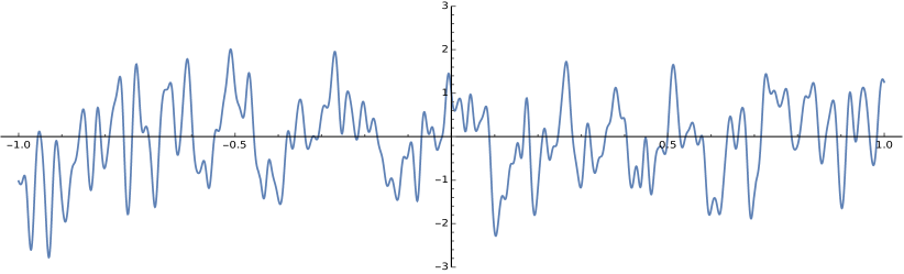
Figure 1. The normalized Weyl polynomial $P_{n}(z)/\sqrt{v_{n}(z)}$ for $z\in(-1,1)$. Here, the degree is $n=10^{4}$ and $\mathbb{P}\left[\xi_{0}=\pm 1\right]=1/2$. In Theorem 2.2, this process will be approximated (in windows of size $\text{const}\cdot n^{-1/2}$) by a stationary Gaussian process.

1.7. Notation

In the following, $C>0$ (respectively, $c>0$) denotes a sufficiently large (respectively, small) constant that does not depend on $n$ and may change from line to line. Usually, our statements hold for sufficiently large $n\geqslant n_{0}$ only, where the number $n_{0}$ also changes from line to line. The floor and the ceiling functions of $x$ are denoted by $\lfloor x\rfloor$ and $\lceil x\rceil$, respectively.

2. Weak convergence to a stationary Gaussian process in a small window

In this section we prove that in a suitable metric space, the appropriately rescaled sequence $(P_{n})_{n\in\mathbb{N}}$ converges weakly to a stationary Gaussian process.

2.1. Metric space of analytic functions

The open and the closed disks of radius $R>0$ will be denoted by

$$\mathbb{D}_{R}=\{z\in\mathbb{C}\colon|z|<R\}\quad\text{and}\quad\overline{\mathbb{D}}_{R}=\{z\in\mathbb{C}\colon|z|\leqslant R\},$$

respectively. Let $A(\mathbb{D}_{R})$ be the space of all functions $f:\overline{\mathbb{D}}_{R}\to\mathbb{C}$ that are continuous on $\overline{\mathbb{D}}_{R}$ and analytic on the open disk $\mathbb{D}_{R}$. Endowed with the uniform norm, $A(\mathbb{D}_{R})$ becomes a Banach space and even a Banach algebra (the disk algebra). Let $A_{\text{real}}(\mathbb{D}_{R})$ be the closed subset of $A(\mathbb{D}_{R})$ consisting of those functions which take real values on $\overline{\mathbb{D}}_{R}\cap\mathbb{R}$.

2.2. The limit process

For $\gamma>0$ let $(Z_{\gamma}(t))_{t\in\mathbb{R}}$ be a stationary, real-valued Gaussian process with zero mean and covariance function

(8) $$\operatorname{Cov}\left[{Z_{\gamma}(s),Z_{\gamma}(t)}\right]=\exp\left(-\frac{\gamma}{2}(t-s)^{2}\right),\quad t,s\in\mathbb{R}.$$

This process can be extended to a random analytic function on the entire complex plane. The probably simplest way to do this is to define

(9) $$Z_{\gamma}(u):={\rm e}^{-\gamma u^{2}/2}\sum_{k=0}^{\infty}\zeta_{k}\frac{\gamma^{k/2}u^{k}}{\sqrt{k!}},\quad u\in\mathbb{C},$$

where $\zeta_{1},\zeta_{2},\ldots$ are i.i.d. real standard Gaussian random variables. Using that $|\zeta_{k}|=O(\sqrt{\log k})$, $k\to\infty$, a.s., it is easy to check that the right-hand side of (9) converges uniformly on compact sets and hence defines an analytic function of $u$, with probability $1$. Then, one easily checks that (8) holds. Moreover, for all $t,s\in\mathbb{C}$ we have

(10) $$\mathbb{E}\left[{Z_{\gamma}(s)Z_{\gamma}(t)}\right]={\rm e}^{-\frac{\gamma}{2}(t-s)^{2}},\quad\mathbb{E}\left[{Z_{\gamma}(s)\overline{Z_{\gamma}(t)}}\right]={\rm e}^{-\frac{\gamma}{2}(\overline{t}-s)^{2}}.$$

The expected number of real zeroes of this stationary Gaussian process is recorded in the next lemma.

Lemma 2.1.

Let $N^{(\gamma)}_{\infty}[a,b]$ be the number of real zeroes of $Z_{\gamma}$ in the interval $[a,b]\subset\mathbb{R}$. Then,

$$\mathbb{E}N_{\infty}^{(\gamma)}[a,b]=\frac{(b-a)}{\pi}\sqrt{\gamma}.$$

Proof.

The covariance function of $Z_{\gamma}$ satisfies

$$\operatorname{Cov}\left[{Z_{\gamma}(0),Z_{\gamma}(t)}\right]={\rm e}^{-\frac{1}{2}\gamma t^{2}}=1-\frac{1}{2}\gamma t^{2}+o(t^{2})\quad\text{ as }t\to 0,$$

and the claim follows from the Rice formula; see for example [9, Chapter 10] or [2, Eq. (3.2) on p. 71]). ∎

2.3. Weak convergence of the random analytic function

Let $P_{n}$ be a random analytic function from one of the four ensembles introduced in Section 1.2. Fix $\delta>0$. We shall show that in a small window of size $\delta n^{-1/2}$ around some point $t\in\mathcal{D}\cap(\mathbb{R}\backslash\{0\})$ the process $P_{n}$ looks, upon a proper rescaling and as $n\to\infty$, like the stationary Gaussian process introduced in (9).

Take some $t\in\mathcal{D}\cap(\mathbb{R}\backslash\{0\})$ and consider the process $Q_{n,t}$ given by

(11) $$Q_{n,t}(z):=\left(v_{n}\left(t+\frac{z}{\sqrt{n}}\right)\right)^{-1/2}P_{n}\left(t+\frac{z}{\sqrt{n}}\right).$$

If we fix some radius $R>0$, then for all sufficiently large $n$, $Q_{n,t}(z)$ is a well-defined random analytic function on $\overline{\mathbb{D}}_{R}$ and we may consider it as a random element of $A_{\rm{real}}(\mathbb{D}_{R})$. Let us now state the functional limit theorem.

Theorem 2.2.

Fix some $t\in\mathcal{D}\cap(\mathbb{R}\backslash\{0\})$. Then, for all $R>0$,

$$Q_{n,t}\overset{\rm w}{\underset{n\to\infty}{\longrightarrow}}Z_{\gamma(t)}\quad\textrm{on }A_{\rm{real}}(\mathbb{D}_{R}),$$

where $\overset{\rm w}{\underset{}{\longrightarrow}}$ denotes weak convergence and $\gamma(t)>0$ is explicitly given by

(12) $$\gamma(t)=\frac{1}{4}\left(\frac{p^{\prime}(t)}{t}+p^{\prime\prime}(t)\right).$$

Remark 2.3.

The theorem breaks down if $t=0$. Indeed, we have $P_{n}(0)=f_{n,0}\xi_{0}$, so there can be no central limit theorem if $\xi_{0}$ is not Gaussian. For other random analytic functions, functional limit theorems of the above type appeared in [28, 3, 24, 16].

Proof of Theorem 2.2.

We can write $Q_{n,t}(z)=\sum_{k=0}^{\infty}a_{n,k}(z)\xi_{k}$, where $a_{n,0}(z),a_{n,1}(z),\ldots$ are analytic functions given by

(13) $$a_{n,k}(z):=\frac{f_{n,k}\left(t+\frac{z}{\sqrt{n}}\right)^{k}}{\sqrt{v_{n}(t+\frac{z}{\sqrt{n}})}},\quad|z|\leqslant R.$$

Convergence of the finite-dimensional distributions. We need to show that for every $d\in\mathbb{N}$ and every $z_{1},\ldots,z_{d}\in\overline{\mathbb{D}}_{R}$,

(14) $$\begin{pmatrix}\operatorname{Re}Q_{n,t}(z_{1})\\ \operatorname{Im}Q_{n,t}(z_{1})\\ \vdots\\ \operatorname{Re}Q_{n,t}(z_{d})\\ \operatorname{Im}Q_{n,t}(z_{d})\end{pmatrix}\overset{\rm d}{\underset{n\to\infty}{\longrightarrow}}\begin{pmatrix}\operatorname{Re}Z_{\gamma(t)}(z_{1})\\ \operatorname{Im}Z_{\gamma(t)}(z_{1})\\ \vdots\\ \operatorname{Re}Z_{\gamma(t)}(z_{d})\\ \operatorname{Im}Z_{\gamma(t)}(z_{d})\end{pmatrix}.$$

The left-hand side can be represented as $\sum_{k=0}^{\infty}V_{n,k}$, where $V_{n,k}$ is the $\mathbb{R}^{2d}$-valued random vector defined by

$$V_{n,k}:=\begin{pmatrix}V_{n,k}(1)\\ V_{n,k}(2)\\ \vdots\\ V_{n,k}(2d-1)\\ V_{n,k}(2d)\end{pmatrix}:=\begin{pmatrix}\operatorname{Re}a_{n,k}(z_{1})\\ \operatorname{Im}a_{n,k}(z_{1})\\ \vdots\\ \operatorname{Re}a_{n,k}(z_{d})\\ \operatorname{Im}a_{n,k}(z_{d})\end{pmatrix}\xi_{k}.$$

We apply the multivariate version of the Lindeberg CLT stated in Proposition 6.2 of [16] to a triangular array whose $n$-th row consists of $V_{n,0},V_{n,1},\ldots$. To prove the convergence of the covariances it suffices to show that for all $z_{i},z_{j}\in\overline{\mathbb{D}}_{R}$,

(15) $$\lim_{n\to\infty}\mathbb{E}\left[Q_{n,t}(z_{i})Q_{n,t}(z_{j})\right] =\mathbb{E}\left[Z_{\gamma(t)}(z_{i})Z_{\gamma(t)}(z_{j})\right],$$

(16) $$\lim_{n\to\infty}\mathbb{E}\left[Q_{n,t}(z_{i})\overline{Q_{n,t}(z_{j})}\right] =\mathbb{E}\left[Z_{\gamma(t)}(z_{i})\overline{Z_{\gamma(t)}(z_{j})}\right],$$

because the covariance matrix of $\sum_{k=0}^{\infty}V_{n,k}$ can be expressed linearly in terms of (15) and (16). For the first expectation we have

(17) $$\mathbb{E}\left[Q_{n,t}(z_{i})Q_{n,t}(z_{j})\right] =\frac{\sum_{k=0}^{\infty}f_{n,k}^{2}\left(t+\frac{z_{i}}{\sqrt{n}}\right)^{k}\left(t+\frac{z_{j}}{\sqrt{n}}\right)^{k}}{\sqrt{v_{n}\left(t+\frac{z_{i}}{\sqrt{n}}\right)v_{n}\left(t+\frac{z_{j}}{\sqrt{n}}\right)}}$$

$$=\frac{v_{n}\left(\sqrt{t^{2}+t\frac{z_{i}+z_{j}}{\sqrt{n}}+\frac{z_{i}z_{j}}{n}}\right)}{\sqrt{v_{n}\left(t+\frac{z_{i}}{\sqrt{n}}\right)v_{n}\left(t+\frac{z_{j}}{\sqrt{n}}\right)}}\sim\frac{\exp\left(np\left(\sqrt{t^{2}+t\frac{z_{i}+z_{j}}{\sqrt{n}}+\frac{z_{i}z_{j}}{n}}\right)\right)}{\exp\left(\frac{n}{2}\left(p\left(t+\frac{z_{i}}{\sqrt{n}}\right)+p\left(t+\frac{z_{j}}{\sqrt{n}}\right)\right)\right)}$$

as $n\to\infty$, where we utilized (6) in the last step. Furthermore, we have

$$\sqrt{t^{2}+t\frac{z_{i}+z_{j}}{\sqrt{n}}+\frac{z_{i}z_{j}}{n}}=t+\frac{z_{i}+z_{j}}{2\sqrt{n}}-\frac{(z_{i}-z_{j})^{2}}{8nt}+o\left(\frac{1}{n}\right),$$

as $n\to\infty$, and since $p$ is supposed to be analytic,

(18) $$p\left(\sqrt{t^{2}+t\frac{z_{i}+z_{j}}{\sqrt{n}}+\frac{z_{i}z_{j}}{n}}\right)=p(t)+p^{\prime}(t)\left(\frac{z_{i}+z_{j}}{2\sqrt{n}}-\frac{(z_{i}-z_{j})^{2}}{8nt}\right)\\ +\frac{p^{\prime\prime}(t)}{2}\frac{(z_{i}+z_{j})^{2}}{4n}+o\left(\frac{1}{n}\right).$$

In addition, we have for $l=i,j$,

(19) $$p\left(t+\frac{z_{l}}{\sqrt{n}}\right)=p(t)+p^{\prime}(t)\frac{z_{l}}{\sqrt{n}}+\frac{p^{\prime\prime}(t)}{2}\frac{z_{l}^{2}}{n}+o\left(\frac{1}{n}\right).$$

Taking (18) and (19) into account and using the identity $\overline{Q_{n,t}(z)}=Q_{n,t}(\overline{z})$, we arrive at

(20) $$\lim_{n\to\infty}\mathbb{E}\left[Q_{n,t}(z_{i})Q_{n,t}(z_{j})\right] =\exp\left(-\frac{1}{2}\gamma(t)(z_{i}-z_{j})^{2}\right),$$

(21) $$\lim_{n\to\infty}\mathbb{E}\left[Q_{n,t}(z_{i})\overline{Q_{n,t}(z_{j})}\right] =\exp\left(-\frac{1}{2}\gamma(t)(z_{i}-\overline{z}_{j})^{2}\right),$$

where

(22) $$\gamma(t):=\frac{1}{4}\left(\frac{p^{\prime}(t)}{t}+p^{\prime\prime}(t)\right).$$

This proves (15) and (16) in view of the formula for the covariance function of $Z_{\gamma}$ given in (10).

It remains to verify the Lindeberg condition, namely

(23) $$\lim_{n\to\infty}\sum_{k=0}^{\infty}\mathbb{E}\left[V_{n,k}^{2}(i)\mathbbm{1}_{\{|V_{n,k}(i)|>\varepsilon\}}\right]=0$$

for all $i=1,\ldots,2d$ and $\varepsilon>0$. Define

$$b_{n,k}:=\max_{i=1,\dots,d}|a_{n,k}(z_{i})|\quad\textrm{and}\quad\tilde{b}_{n}:=\max_{k=0,1,\ldots}b_{n,k}.$$

Then, $V_{n,k}^{2}(i)\leqslant b_{n,k}^{2}\xi_{k}^{2}$ for all $i=1,\ldots,2d$ and thus, for every $\varepsilon>0$,

$$\sum_{k=0}^{\infty}\mathbb{E}\left[V^{2}_{n,k}(i)\mathbbm{1}_{\{|V_{n,k}(i)|>\varepsilon\}}\right] \leqslant\sum_{k=0}^{\infty}b_{n,k}^{2}\mathbb{E}\left[\xi_{k}^{2}\mathbbm{1}_{\{|\xi_{k}|>\varepsilon/b_{n,k}\}}\right]$$

$$\leqslant\mathbb{E}\left[\xi_{1}^{2}\mathbbm{1}_{\{|\xi_{1}|>\varepsilon/\tilde{b}_{n}\}}\right]\sum_{k=0}^{\infty}b_{n,k}^{2}$$

$$\leqslant\mathbb{E}\left[\xi_{1}^{2}\mathbbm{1}_{\{|\xi_{1}|>\varepsilon/\tilde{b}_{n}\}}\right]\sum_{k=0}^{\infty}\sum_{j=1}^{d}|a_{n,k}(z_{j})|^{2}$$

$$\leqslant C\,\mathbb{E}\left[\xi_{1}^{2}\mathbbm{1}_{\{|\xi_{1}|>\varepsilon/\tilde{b}_{n}\}}\right].$$

In the last step we used that for all $j=1,\dots,d$,

$$\sum_{k=0}^{\infty}|a_{n,k}(z_{j})|^{2}=\mathbb{E}[Q_{n,t}(z_{j})\overline{Q_{n,t}(z_{j})}]\overset{}{\underset{n\to\infty}{\longrightarrow}}\exp\left(2\gamma(t)(\operatorname{Im}z_{j})^{2}\right),\quad\text{ as }n\to\infty,$$

by (21). Finally,

$$\lim_{n\to\infty}\mathbb{E}\left[\xi_{1}^{2}\mathbbm{1}_{\{|\xi_{1}|>\varepsilon/\tilde{b}_{n}\}}\right]=0$$

because $\mathbb{E}\left[\xi_{1}^{2}\right]=1<\infty$ and $\lim_{n\to\infty}\tilde{b}_{n}=0$ by Lemma 5.1 whose statement and proof are postponed to Section 5. This verifies the Lindeberg condition (23) and completes the proof of (14).

Tightness. To complete the proof of the theorem we need to show that the probability laws of $(Q_{n,t})_{n\in\mathbb{N}}$ form a tight sequence on $A_{\rm{real}}(\mathbb{D}_{R})$. For random analytic functions, there are especially simple criteria of tightness. Namely, by [40, Remark on p. 341], it suffices to show that $\mathbb{E}|Q_{n,t}(z)|^{2}\leqslant C$ for all $z\in\overline{\mathbb{D}}_{R}$ and all sufficiently large $n\in\mathbb{N}$. But (21) (which holds uniformly over $z_{i},z_{j}\in\overline{\mathbb{D}}_{R}$) yields

(24) $$\mathbb{E}\left|Q_{n,t}(z)\right|^{2}=\mathbb{E}\left[Q_{n,t}(z)\overline{Q_{n,t}(z)}\right]=\exp\left(2\gamma(t)(\operatorname{Im}z)^{2}+o(1)\right)<C,$$

thus completing the proof of Theorem 2.2. ∎

2.4. Distributional convergence of the number of zeroes

The next lemma transfers the weak convergence of the scaled random analytic functions $Q_{n,t}$ on $A_{\rm{real}}(\mathbb{D}_{R})$ to the convergence in distribution of the corresponding random number of zeroes in small windows of length $\delta/\sqrt{n}$.

Lemma 2.4.

Fix some $\delta>0$ and $t\in\mathcal{D}\cap(\mathbb{R}\backslash\{0\})$. Then, the sequence of random variables

(25) $$\left(N_{n}\left[t,t+\frac{\delta}{\sqrt{n}}\right]\right)_{n\in\mathbb{N}}$$

converges in distribution to the number of real zeroes of the Gaussian process $Z_{\gamma(t)}(\cdot)$ in the interval $[0,\delta]$.

Proof.

By (11), $N_{n}[t,t+\delta/\sqrt{n}]$ is the number of real zeroes of $Q_{n,t}(\cdot)$ in the interval $[0,\delta]$. By Theorem 2.2, the latter process converges weakly to $Z_{\gamma(t)}(\cdot)$ on the space $A_{\rm{real}}(\mathbb{D}_{R})$, as $n\to\infty$. We may take $R>\delta$, so that the interval $[0,\delta]$ is contained in the interior of the disk $\mathbb{D}_{R}$ of radius $R$. To pass to the distributional convergence of real zeroes, we employ the continuous mapping theorem in the same way as it was done in [24]. By Lemma 4.1 therein, the map which assigns to a function $f\in A_{\rm{real}}(\mathbb{D}_{R})\backslash\{0\}$ the number of zeroes of $f$ in the interval $[0,\delta]$ is locally constant (hence, continuous) on the set of all analytic functions which do not vanish at $0,\delta$ and have no multiple zeroes in the interval $[0,\delta]$. This set has full measure w.r.t. the law of $Z_{\gamma(t)}$ (the a.s. absence of multiple zeroes follows from the Bulinskaya lemma; see, e.g., [24, Lemma 4.3]). Hence, the continuous mapping theorem implies the distributional convergence of $N_{n}[t,t+\delta/\sqrt{n}]$ to the number of zeroes of $Z_{\gamma(t)}$ in $[0,\delta]$ as $n\to\infty$. ∎

2.5. Proof of Theorem 1.1 assuming uniform integrability

As we shall prove in Lemma 3.1, below, the sequence (25) is uniformly integrable for $0<\delta<1/2$. Assuming this, we can prove Theorem 1.1 as follows. Let $\varepsilon_{0}>0$ be so small that the interval $[a-2\varepsilon_{0},b+2\varepsilon_{0}]$ is contained in $\mathcal{D}\cap(\mathbb{R}\backslash\{0\})$. Define a function $g_{n}:[a-\varepsilon_{0},b+\varepsilon_{0}]\to[0,\infty)$ as follows:

$$g_{n}(t)=\mathbb{E}N_{n}\left[t,t+\frac{\delta}{\sqrt{n}}\right].$$

It follows from this definition that for sufficiently large $n$,

(26) $$\int_{a}^{b-(\delta/\sqrt{n})}g_{n}(t)\ \mathrm{d}t\leqslant\frac{\delta}{\sqrt{n}}\mathbb{E}N_{n}[a,b]\leqslant\int_{a-(\delta/\sqrt{n})}^{b}g_{n}(t)\ \mathrm{d}t.$$

The distributional convergence stated in Lemma 2.4 and the uniform integrability implied by Lemma 3.1 yield the convergence of the expectations:

(27) $$\lim_{n\to\infty}g_{n}(t)=\lim_{n\to\infty}\mathbb{E}N_{n}\left[t,t+\frac{\delta}{\sqrt{n}}\right]=\mathbb{E}N_{\infty}^{(\gamma(t))}[0,\delta]=\frac{\delta}{\pi}\sqrt{\gamma(t)}=\frac{\delta}{2\pi}\sqrt{\frac{p^{\prime}(t)}{t}+p^{\prime\prime}(t)}$$

for all $t\in[a-\varepsilon_{0},b+\varepsilon_{0}]$; see also Lemma 2.1 for the expected number of zeroes of the limit process. Also, it follows from Lemma 3.1 that $0\leqslant g_{n}(t)\leqslant C$ for some constant $C>0$ and all sufficiently large $n$. Utilizing the dominated convergence theorem, we arrive at

$$\lim_{n\to\infty}\int_{a}^{b-(\delta/\sqrt{n})}g_{n}(t)\ \mathrm{d}t=\lim_{n\to\infty}\int_{a-(\delta/\sqrt{n})}^{b}g_{n}(t)\ \mathrm{d}t=\frac{\delta}{2\pi}\int\limits_{a}^{b}\sqrt{\frac{p^{\prime}(t)}{t}+p^{\prime\prime}(t)}\ \mathrm{d}t.$$

The sandwich lemma, applied to (26), yields

$$\lim_{n\to\infty}\frac{\mathbb{E}N_{n}[a,b]}{\sqrt{n}}=\frac{1}{2\pi}\int\limits_{a}^{b}\sqrt{\frac{p^{\prime}(t)}{t}+p^{\prime\prime}(t)}\ \mathrm{d}t,$$

thus completing the proof of Theorem 1.1.

3. Uniform integrability of $N_{n}$ on intervals of length $\delta n^{-1/2}$

3.1. Statement of the main lemmas

We recall that $N_{n}[a,b]$ is the number of real zeroes of $P_{n}$ (defined by (1) and (2)) in the interval $[a,b]\subset\mathcal{D}\cap\mathbb{R}$. We aim to prove the following

Lemma 3.1.

Fix some $0<\delta<1/2$ and a compact set $K\subset\mathcal{D}\cap(\mathbb{R}\backslash\{0\})$. Let also $1<\kappa<2$. Then there exists a constant $C>0$ such that for all sufficiently large $n\in\mathbb{N}$ and all $t\in K$,

$$\mathbb{E}\left[N^{\kappa}_{n}\left[t,t+\frac{\delta}{\sqrt{n}}\right]\right]<C.$$

We shall deduce Lemma 3.1 from the following two statements whose proofs are postponed:

Lemma 3.2.

Fix $1<\kappa<2$, an interval $[a,b]\subset\mathcal{D}\cap\mathbb{R}$ and $\varepsilon>0$. Then,

$$\lim_{n\to\infty}\mathbb{E}\left[N^{\kappa}_{n}[a,b]\mathbbm{1}_{\{N_{n}[a,b]\geqslant\mathrm{e}^{n^{\varepsilon}}\}}\right]=0.$$

Lemma 3.3.

Fix some sufficiently small $0<\delta<1/2$ and a compact set $K\subset\mathcal{D}\cap(\mathbb{R}\backslash\{0\})$. Then there exist constants $C>0$ and $c>0$ such that

$$\mathbb{P}\left[N_{n}[t,t+\delta n^{-1/2}]\geqslant m\right]\leqslant C\left(\left(2\delta\right)^{(2/3)m}+\left(2\delta\right)^{-(1/3)m}\exp\left(-cn^{1/5}\right)\right)$$

for all $n\geqslant n_{0}$, $m\in\mathbb{N}$, and $t\in K$.

Proof of Lemma 3.1 given Lemmas 3.2 and 3.3.

For $t\in K$ we write

$$N_{n,t,\delta}:=N_{n}\left[t,t+\frac{\delta}{\sqrt{n}}\right].$$

We can find an interval $[a,b]\subset\mathcal{D}\cap\mathbb{R}$ such that $K\subset(a,b)$. Take some $\varepsilon>0$. Then, for sufficiently large $n$, we have $N_{n,t,\delta}\leqslant N_{n}[a,b]$ and hence

$$\mathbb{E}\left[N^{\kappa}_{n,t,\delta}\mathbbm{1}_{\{N_{n,t,\delta}\geqslant\mathrm{e}^{n^{\varepsilon}}\}}\right]\leqslant\mathbb{E}\left[N^{\kappa}_{n}[a,b]\mathbbm{1}_{\{N_{n}[a,b]\geqslant\mathrm{e}^{n^{\varepsilon}}\}}\right]<C$$

in view of Lemma 3.2. Thus, it suffices to show that $\mathbb{E}\left[N^{\kappa}_{n,t,\delta}\mathbbm{1}_{\{N_{n,t,\delta}\leqslant\mathrm{e}^{n^{\varepsilon}}\}}\right]<C$. Let $m_{0}=m_{0}(n,\delta)$ be chosen such that

(28) $$\exp\left(\frac{c}{4}n^{1/5}\right)\leqslant(2\delta)^{-m_{0}/3}\leqslant\exp\left(\frac{c}{2}n^{1/5}\right),$$

where $c>0$ is the small constant from Lemma 3.3. It follows from (28) that

(29) $$(2\delta)^{2m_{0}/3}\leqslant\exp\left(-\frac{c}{2}n^{1/5}\right).$$

Observe that $\{N_{n}[t,t+\delta n^{-1/2}]\geqslant 1\}\supseteq\{N_{n}[t,t+\delta n^{-1/2}]\geqslant 2\}\supseteq\ldots$ is a non-increasing sequence of events. Therefore,

$$\mathbb{E}\left[N^{\kappa}_{n,t,\delta}\mathbbm{1}_{\{N_{n,t,\delta}\leqslant\mathrm{e}^{n^{\varepsilon}}\}}\right]\leqslant\mathbb{E}\left[N^{2}_{n,t,\delta}\mathbbm{1}_{\{N_{n,t,\delta}\leqslant\mathrm{e}^{n^{\varepsilon}}\}}\right]\leqslant\sum_{m=1}^{\lfloor\mathrm{e}^{n^{\varepsilon}}\rfloor}(2m-1)\mathbb{P}\left[N_{n}[t,t+\delta n^{-1/2}]\geqslant m\right]\\ \leqslant\sum_{m=1}^{m_{0}}(2m-1)\mathbb{P}\left[N_{n}[t,t+\delta n^{-1/2}]\geqslant m\right]+\mathbb{P}\left[N_{n}[t,t+\delta n^{-1/2}]\geqslant m_{0}\right]\sum_{m=m_{0}+1}^{\lfloor\mathrm{e}^{n^{\varepsilon}}\rfloor}(2m-1),$$

where we observe that $m_{0}<{\rm e}^{n^{\varepsilon}}$ for sufficiently large $n$, as follows from (28). Applying Lemma 3.3 we obtain, for sufficiently small $\varepsilon>0$,

$$\mathbb{E}\left[N^{\kappa}_{n,t,\delta}\mathbbm{1}_{\{N_{n,t,\delta}\leqslant\mathrm{e}^{n^{\varepsilon}}\}}\right] \leqslant C\sum_{m=1}^{\infty}(2m-1)\left(2\delta\right)^{2m/3}+C\exp\left(-cn^{1/5}\right)\sum_{m=1}^{\lfloor\mathrm{e}^{n^{\varepsilon}}\rfloor}(2m-1)\left(2\delta\right)^{-1/3m}$$

$$\quad+C\mathrm{e}^{2n^{\varepsilon}}\left((2\delta)^{2m_{0}/3}+(2\delta)^{-m_{0}/3}\exp\left(-cn^{1/5}\right)\right)$$

$$\leqslant C+C\mathrm{e}^{2n^{\varepsilon}}\exp\left(-\frac{c}{2}n^{1/5}\right)<C,$$

where we used (28) and (29). ∎

3.2. Proof of Lemma 3.2

We fix $1<\kappa<2$, an interval $[a,b]\subset\mathcal{D}\cap\mathbb{R}$ and $\varepsilon>0$. Our aim is to prove that

(30) $$\lim_{n\to\infty}\mathbb{E}\left[N^{\kappa}_{n}[a,b]\mathbbm{1}_{\{N_{n}[a,b]\geqslant\mathrm{e}^{n^{\varepsilon}}\}}\right]=0.$$

Proof of (30).

First of all, the statement is trivial for spherical and Weyl polynomials because the number of real zeroes of a degree $n$ polynomial is bounded by $n$. In the following, we consider the FAF and the HAF cases only. In particular, the coefficients $f_{n,k}$ do not vanish. The first step of the proof uses an argument based on the Jensen theorem which follows an idea of [22] as developed in [16]. Since $\mathbb{P}\left[\xi_{0}=0\right]\neq 1$, we can choose a sufficiently small $0<\eta<1$ such that

$$q:=\mathbb{P}\left[|\xi_{0}|\leqslant\mathrm{e}\eta\right]<1.$$

For $k=0,1,\dots$ consider the events

$$B_{k}:=\left\{|\xi_{0}|\leqslant\mathrm{e}\eta,\dots,|\xi_{k-1}|\leqslant\mathrm{e}\eta,|\xi_{k}|>\mathrm{e}\eta\right\}.$$

Keep in mind that

$$\quad\mathbb{P}\left[B_{k}\right]=q^{k}(1-q)\quad\textrm{and}\quad\bigcup_{k=0}^{\infty}B_{k}=\Omega\mod\mathbb{P},$$

where $(\Omega,\mathcal{A},\mathbb{P})$ is the probability space we are working on. Let $P_{n}^{(k)}$ denote the $k$-th derivative of $P_{n}$. On the event $B_{k}$ we have

$$\left|P_{n}^{(k)}(0)\right|=k!f_{n,k}|\xi_{k}|\geqslant k!f_{n,k}\mathrm{e}\eta\geqslant k!f_{n,k}\eta.$$

We shall use the abbreviation $N_{n}=N_{n}[a,b]$. By the theorem of Rolle, $N_{n}$ can be upperbounded by the number of zeroes of $P_{n}^{(k)}$ in the interval $[a,b]$ plus $k$. Choosing $r:=\max\{|a|,|b|\}$, we can estimate $N_{n}$ by the number of zeroes of $P_{n}^{(k)}$ in the disk $\bar{\mathbb{D}}_{r}$ plus $k$. Jensen’s theorem (see, e.g. [8, pp. 280–281]) applied to $P_{n}^{(k)}$ yields that on the event $B_{k}$,

(31) $$N_{n}\leqslant k+\frac{1}{\log\left(R/r\right)}\log\left(\frac{\sup_{|z|=R}{|P_{n}^{(k)}(z)|}}{|P_{n}^{(k)}(0)|}\right)\\ \leqslant k+C\log\left(\frac{1}{\eta}\sum_{j=k}^{\infty}\binom{j}{k}\frac{f_{n,j}}{f_{n,k}}|\xi_{j}|R^{j-k}\right),$$

where we have chosen $R$ such that $r<R\in\mathcal{D}\cap\mathbb{R}$. Besides, on $B_{k}$ we have

(32) $$\frac{1}{\eta}\sum_{j=k}^{\infty}\binom{j}{k}\frac{f_{n,j}}{f_{n,k}}|\xi_{j}|R^{j-k}\geqslant\frac{|\xi_{k}|}{\eta}\geqslant\mathrm{e}.$$

On the other hand, we shall show in Lemma 5.2, below, that there is $C>0$ such that for all $n\in\mathbb{N}$, $k\in\mathbb{N}_{0}$,

(33) $$\sum_{j=k}^{\infty}\binom{j}{k}\frac{f_{n,j}}{f_{n,k}}R^{j-k}\leqslant\frac{C}{f_{n,k}}\left(\frac{2}{R\log(A/R)}\right)^{k}\exp\left(\frac{n}{2}p\left(\sqrt{AR}\right)\right),$$

where $R<A\in\mathcal{D}\cap\mathbb{R}$ is a constant independent of $n$ and $k$ and $p:\mathcal{D}\to\mathbb{C}$ is given by (7). Using the same idea as in the standard proof of the Markov inequality, we obtain the estimate

$$\mathbb{E}\left[N_{n}^{\kappa}\mathbbm{1}_{\left\{N_{n}\geqslant\mathrm{e}^{n^{\varepsilon}}\right\}\cap B_{k}}\right] =\mathbb{E}\left[\frac{N_{n}^{2}}{N_{n}^{2-\kappa}}\mathbbm{1}_{\left\{N_{n}\geqslant\mathrm{e}^{n^{\varepsilon}}\right\}\cap B_{k}}\right]\leqslant\mathbb{E}\left[\frac{N_{n}^{2}}{\mathrm{e}^{n^{\varepsilon}(2-\kappa)}}\mathbbm{1}_{\left\{N_{n}\geqslant\mathrm{e}^{n^{\varepsilon}}\right\}\cap B_{k}}\right]$$

$$\leqslant\mathrm{e}^{-n^{\varepsilon}(2-\kappa)}\mathbb{E}\left[N^{2}_{n}\mathbbm{1}_{B_{k}}\right]$$

which holds for all $k=0,1,\ldots$. The inequality $(a+b)^{2}\leqslant 2a^{2}+2b^{2}$, for all $a,b\in\mathbb{R}$, combined with (31) allows us to conclude that

(34) $$\mathbb{E}\left[N_{n}^{\kappa}\mathbbm{1}_{\left\{N_{n}\geqslant\mathrm{e}^{n^{\varepsilon}}\right\}\cap B_{k}}\right]\leqslant C\mathrm{e}^{-n^{\varepsilon}(2-\kappa)}\left(k^{2}\mathbb{P}\left[B_{k}\right]+\mathbb{E}\left[\log^{2}\left(\frac{1}{\eta}\sum_{j=k}^{\infty}\binom{j}{k}|\xi_{j}|\frac{f_{n,j}}{f_{n,k}}R^{j-k}\right)\mathbbm{1}_{B_{k}}\right]\right).$$

Since the function $x\mapsto\log^{2}(x)$ is concave for $x\geqslant\mathrm{e}$ and in view of (32), we may use the inequality of Jensen (on the event $B_{k}$) to obtain the estimate

$$\mathbb{E}\left[\log^{2}\left(\frac{1}{\eta}\sum_{j=k}^{\infty}\binom{j}{k}|\xi_{j}|\frac{f_{n,j}}{f_{n,k}}R^{j-k}\right)\mathbbm{1}_{B_{k}}\right]\leqslant\mathbb{P}\left[B_{k}\right]\log^{2}\left(\frac{1}{\mathbb{P}\left[B_{k}\right]}\mathbb{E}\left[\frac{1}{\eta}\sum_{j=k}^{\infty}\binom{j}{k}|\xi_{j}|\frac{f_{n,j}}{f_{n,k}}R^{j-k}\mathbbm{1}_{B_{k}}\right]\right).$$

Treating the term with $j=k$ separately, using the independence of $(\xi_{k})_{k\in\mathbb{N}_{0}}$, the observation $\mathbb{E}\left[|\xi_{j}|\mathbbm{1}_{B_{k}}\right]=\mathbb{P}\left[B_{k}\right]\mathbb{E}|\xi_{1}|\leqslant\mathbb{P}\left[B_{k}\right]$ for $j>k$, and (33), we obtain for sufficiently large $n$ the estimate

(35) $$\begin{split}&\mathbb{E}\left[\log^{2}\left(\frac{1}{\eta}\sum_{j=k}^{\infty}\binom{j}{k}|\xi_{j}|\frac{f_{n,j}}{f_{n,k}}R^{j-k}\right)\mathbbm{1}_{B_{k}}\right]\\ &\leqslant\mathbb{P}\left[B_{k}\right]\log^{2}\left(\frac{\mathbb{E}\left[|\xi_{k}|\mathbbm{1}_{B_{k}}\right]}{\eta\mathbb{P}\left[B_{k}\right]}+\frac{1}{\mathbb{P}\left[B_{k}\right]}\mathbb{E}\left[\frac{1}{\eta}\sum_{j=k+1}^{\infty}\binom{j}{k}|\xi_{j}|\frac{f_{n,j}}{f_{n,k}}R^{j-k}\mathbbm{1}_{B_{k}}\right]\right)\\ &\leqslant\mathbb{P}\left[B_{k}\right]\log^{2}\left(\frac{\mathbb{E}\left[|\xi_{k}|\mathbbm{1}_{\{|\xi_{k}|>\mathrm{e}\eta\}}\prod_{l=0}^{k-1}\mathbbm{1}_{\{|\xi_{l}|\leqslant\mathrm{e}\eta\}}\right]}{\eta q^{k}(1-q)}+\frac{1}{\eta}\sum_{j=k+1}^{\infty}\binom{j}{k}\frac{f_{n,j}}{f_{n,k}}R^{j-k}\right)\\ &\leqslant\mathbb{P}\left[B_{k}\right]\log^{2}\left(\frac{\mathbb{E}\left[|\xi_{k}|\mathbbm{1}_{\{|\xi_{k}|>\mathrm{e}\eta\}}\right]}{\eta(1-q)}+\frac{C}{\eta f_{n,k}}\left(\frac{2}{R\log(A/R)}\right)^{k}\mathrm{e}^{np(\sqrt{AR})/2}\right)\\ &\leqslant\mathbb{P}\left[B_{k}\right]\log^{2}\left(C+\frac{C}{\eta f_{n,k}}\left(\frac{2}{R\log(A/R)}\right)^{k}\mathrm{e}^{np(\sqrt{AR})/2}\right).\end{split}$$

We have to estimate the right-hand side. Recall that

$$f^{2}_{n,k}=\begin{cases}\frac{n^{k}}{k!}&\textrm{in the {FAF}\ case,}\\ \binom{n+k-1}{k}&\textrm{in the {HAF}\ case}.\end{cases}$$

In the FAF case, we can use the inequality $(a+b)^{2}\leqslant 2(a^{2}+b^{2})$ to obtain the estimate

(36) $$\log^{2}(f^{2}_{n,k})=\left(k\log n-\log(k!)\right)^{2}\leqslant 2k^{2}\log^{2}n+2\log^{2}(k!)\leqslant C(k^{4}+1)n^{2}.$$

In the HAF case, we have

(37) $$\log^{2}(f^{2}_{n,k})=\log^{2}\left(\binom{n+k-1}{k}\right)\leqslant\log^{2}\left((n+k)!\right)\leqslant C(n+k)^{4}\leqslant 8C(n^{4}+k^{4}).$$

Taking together the estimates (36) and (37) we obtain the following estimate which is valid both for HAF and FAF:

(38) $$\log^{2}(f^{2}_{n,k})\leqslant C(k^{4}+1)n^{4}\quad\textrm{for all }k\in\mathbb{N}_{0},n\in\mathbb{N}.$$

For a given $C>1$ there exists a constant $\tilde{C}>0$ such that $\log^{2}(C+x)\leqslant\log^{2}x+\tilde{C}$ for all $x>0$. Using this observation together with the estimate (38) and the inequality $(a+b+c+d)^{2}\leqslant 4(a^{2}+b^{2}+c^{2}+d^{2})$, we can estimate the right-hand side of (35) as follows:

$$\mathbb{P}\left[B_{k}\right]\log^{2}\left(C+\frac{C}{\eta f_{n,k}}\left(\frac{2}{R\log(A/R)}\right)^{k}\mathrm{e}^{np(\sqrt{AR})/2}\right)$$

$$\leqslant\tilde{C}\mathbb{P}\left[B_{k}\right]+\mathbb{P}\left[B_{k}\right]\log^{2}\left(\frac{C}{\eta f_{n,k}}\left(\frac{2}{R\log(A/R)}\right)^{k}\mathrm{e}^{np(\sqrt{AR})/2}\right)$$

$$=\tilde{C}\mathbb{P}\left[B_{k}\right]+\mathbb{P}\left[B_{k}\right]\left(\log\frac{C}{\eta}-\frac{1}{2}\log\left(f_{n,k}^{2}\right)+k\log\left(\frac{2}{R\log(A/R)}\right)+\frac{n}{2}p\left(\sqrt{AR}\right)\right)^{2}$$

$$\leqslant\tilde{C}\mathbb{P}\left[B_{k}\right]+4\mathbb{P}\left[B_{k}\right]\left(\log^{2}\frac{C}{\eta}+\frac{1}{4}\log^{2}\left(f_{n,k}^{2}\right)+k^{2}\log^{2}\left(\frac{2}{R\log(A/R)}\right)+\frac{n^{2}}{4}p^{2}\left(\sqrt{AR}\right)\right)$$

$$\leqslant C\mathbb{P}\left[B_{k}\right](k^{4}+1)n^{4},$$

where in the last step we estimated terms of the form $1,k^{2},n^{2}$ by $n^{4},k^{4}n^{4},n^{4}$, respectively. Combining this with the above estimates (34) and (35) yields

$$\mathbb{E}\left[N_{n}^{\kappa}\mathbbm{1}_{\left\{N_{n}\geqslant\mathrm{e}^{n^{\varepsilon}}\right\}}\mathbbm{1}_{B_{k}}\right]\leqslant C\mathrm{e}^{-n^{\varepsilon}(2-\kappa)}\mathbb{P}\left[B_{k}\right](k^{4}+1)n^{4}=C\mathrm{e}^{-n^{\varepsilon}(2-\kappa)}n^{4}(k^{4}+1)q^{k}(1-q).$$

Therefore, taking the sum over $k=0,1,\ldots$, we arrive at

$$\mathbb{E}\left[N_{n}^{\kappa}\mathbbm{1}_{\left\{N_{n}\geqslant\mathrm{e}^{n^{\varepsilon}}\right\}}\right]=\sum_{k=0}^{\infty}\mathbb{E}\left[N_{n}^{\kappa}\mathbbm{1}_{\left\{N_{n}\geqslant\mathrm{e}^{n^{\varepsilon}}\right\}}\mathbbm{1}_{B_{k}}\right]\leqslant C\mathrm{e}^{-n^{\varepsilon}(2-\kappa)}n^{4}\sum_{k=0}^{\infty}(k^{4}+1)q^{k}(1-q).$$

The right-hand side converges to $0$ as $n\to\infty$ because the sum is a finite constant. This completes the proof of (30). ∎

3.3. Proof of Lemma 3.3

Fix some sufficiently small $0<\delta<1/2$, some $1<\kappa<2$ and a compact set $K\subset\mathcal{D}\cap(\mathbb{R}\backslash\{0\})$. Our aim is to prove that there exist constants $C>0$ and $c>0$ such that

(39) $$\mathbb{P}\left[N_{n}[t,t+\delta n^{-1/2}]\geqslant m\right]\leqslant C\left(\left(2\delta\right)^{(2/3)m}+\left(2\delta\right)^{-(1/3)m}\exp\left(-cn^{1/5}\right)\right)\quad\textrm{for all }n,m\in\mathbb{N},\textrm{ for all }t\in K.$$

Proof of (39).

Recall from (11) that the process $Q_{n,t}$ is given by

$$Q_{n,t}(z)=\left(v_{n}\left(t+\frac{z}{\sqrt{n}}\right)\right)^{-1/2}P_{n}\left(t+\frac{z}{\sqrt{n}}\right).$$

For $T>0$ and $m\in\mathbb{N}$ we write

(40) $$\mathbb{P}\left[N_{n}[t,t+\delta n^{-1/2}]\geqslant m\right]\leqslant\mathbb{P}\left[N_{n}[t,t+\delta n^{-1/2}]\geqslant m,\left|Q_{n,t}(0)\right|\geqslant T\right]+\mathbb{P}\left[\left|Q_{n,t}(0)\right|<T\right]$$

and estimate the terms on the right-hand side separately.

The first term on the right-hand side of (40) will be estimated by using a lemma of Ibragimov and Maslova [22]; see also [16, Lemma 4.4] for the proof in the generality needed here. In our setting, this lemma states that

$$\mathbb{P}\left[N_{n}[t,t+\delta n^{-1/2}]\geqslant m,\left|Q_{n,t}(0)\right|\geqslant T\right]\leqslant\frac{\delta^{2m}}{(m!)^{2}T^{2}}\sup_{x\in[0,\delta]}\mathbb{E}\left|Q^{(m)}_{n,t}(x)\right|^{2},$$

where $Q^{(m)}_{n,t}$ denotes the $m$-th derivative of $Q_{n,t}$. Since for sufficiently large $n$, the function $(Q_{n,t}(z))_{|z|<2}$ is analytic, Cauchy’s integral formula for analytic functions yields, for all $x\in[0,\delta]$,

$$\left|Q^{(m)}_{n,t}(x)\right|=\frac{m!}{2\pi}\left|\oint_{\partial\mathbb{D}}\frac{Q_{n,t}(z)}{(z-x)^{m+1}}\ \mathrm{d}z\right|\leqslant\frac{m!}{2\pi}\int_{\partial\mathbb{D}}\frac{|Q_{n,t}(z)|}{(1-\delta)^{m+1}}\ |\mathrm{d}z|,$$

where $\partial\mathbb{D}=\{|z|=1\}$ is the unit circle. After squaring, taking the expectation and using Jensen’s inequality for the quadratic function two times we obtain

$$\mathbb{E}\left|Q_{n,t}^{(m)}(x)\right|^{2} \leqslant\frac{(m!)^{2}}{4\pi^{2}(1-\delta)^{2m+2}}\mathbb{E}\left(\int_{\partial\mathbb{D}}|Q_{n,t}(z)|\ |\mathrm{d}z|\right)^{2}$$

$$\leqslant\frac{(m!)^{2}}{2\pi(1-\delta)^{2m+2}}\mathbb{E}\int_{\partial\mathbb{D}}|Q_{n,t}(z)|^{2}\ |\mathrm{d}z|$$

$$\leqslant\frac{(m!)^{2}}{2\pi(1-\delta)^{2m+2}}\int_{\partial\mathbb{D}}\mathbb{E}|Q_{n,t}(z)|^{2}\ |\mathrm{d}z|$$

$$\leqslant\frac{(m!)^{2}}{(1-\delta)^{2m+2}}\sup_{z\in\partial\mathbb{D}}\mathbb{E}|Q_{n,t}(z)|^{2}.$$

Since the above holds for arbitrary $x\in[0,\delta]$, it follows that

$$\sup_{x\in[0,\delta]}\mathbb{E}\left|Q^{(m)}_{n,t}(x)\right|^{2}\leqslant\frac{(m!)^{2}}{2\pi(1-\delta)^{2m+2}}\sup_{|z|\leqslant 1}\mathbb{E}\left|Q_{n,t}(z)\right|^{2}.$$

Using the estimate given in (24) (with $R=1$) we find a constant $C>0$ such that

$$\mathbb{E}\left|Q_{n,t}(z)\right|^{2}\leqslant C\quad\textrm{for all }|z|\leqslant 1,\;\;n\in\mathbb{N},\;\;t\in K.$$

Taking everything together yields the following estimate for the first term on the right-hand side of (40):

(41) $$\mathbb{P}\left[N_{n}[t,t+\delta n^{-1/2}]\geqslant m,\left|Q_{n,t}(0)\right|\geqslant T\right]\leqslant\frac{C}{T^{2}}\frac{\delta^{2m}}{(1-\delta)^{2(m+1)}}\leqslant\frac{C}{T^{2}}\left(\frac{\delta}{1-\delta}\right)^{2m}\leqslant\frac{C}{T^{2}}\left(2\delta\right)^{2m},$$

for every $T>0$, where we used that $0<\delta<1/2$ in the last step.

The second term on the right-hand side of (40) will be estimated in Lemma 4.1, below, which states that

$$\mathbb{P}\left[\left|Q_{n,t}(0)\right|<T\right]\leqslant C\left(T+T^{-1/2}\exp\left(-cn^{1/5}\right)\right).$$

Taking the estimates for both terms on the right-hand side of (40) together, we obtain

$$\mathbb{P}\left[N_{n}[t,t+\delta n^{-1/2}]\geqslant m\right]\leqslant C\left(\frac{\left(2\delta\right)^{2m}}{T^{2}}+T+T^{-1/2}\exp\left(-cn^{1/5}\right)\right).$$

Optimizing the bound by choosing $T=(2\delta)^{(2/3)m}$ completes the proof of (39). ∎

4. Estimating the probability of small values of $P_{n}$

Recall from (11) that

$$Q_{n,t}(0)=\frac{P_{n}(t)}{\sqrt{v_{n}(t)}}=\sum_{k=0}^{\infty}\frac{f_{n,k}t^{k}}{\sqrt{v_{n}(t)}}\xi_{k}.$$

The main result of the present section is the following lemma that estimates the probabilities of small values of $Q_{n,t}(0)$.

Lemma 4.1.

Fix a compact set $K\subset\mathcal{D}\cap(\mathbb{R}\backslash\{0\})$. There exist constants $C=C(K)>0$ and $c=c(K)>0$ such that

$$\mathbb{P}\left[\left|Q_{n,t}(0)\right|<T\right]\leqslant C\left(T+T^{-1/2}\exp\left(-cn^{1/5}\right)\right)$$

for all $T>0$, $n\geqslant n_{0}$ and for all $t\in K$.

Proof.

The first step is a smoothing argument similar to that used by Ibragimov and Maslova [22]. Take some $\lambda>0$ (to be chosen explicitly at the very end of the proof) and consider the random variable

$$\tilde{Q}_{n}:=Q_{n,t}(0)+\Theta_{\lambda},$$

where $\Theta_{\lambda}$ is the sum of two independent random variables that are uniformly distributed on the interval $[-\lambda,\lambda]$ and independent of $Q_{n,t}(0)$. The characteristic function of $\Theta_{\lambda}$ is given by

$$\psi_{\lambda}(u):=\mathbb{E}\left[\exp\left(\mathrm{i}u\Theta_{\lambda}\right)\right]=\frac{\sin^{2}(u\lambda)}{u^{2}\lambda^{2}}.$$

For $T>0$ we have the estimate

(42) $$\mathbb{P}\left[\left|Q_{n,t}(0)\right|\leqslant T\right]\leqslant\mathbb{P}\left[\left|\tilde{Q}_{n}\right|\leqslant\frac{3}{2}T\right]+\mathbb{P}\left[|\Theta_{\lambda}|\geqslant\frac{1}{2}T\right].$$

In the following we shall estimate the two terms on the right-hand side of (42).

Second term of on the right-hand side of (42). By Chebyshev’s inequality,

(43) $$\mathbb{P}\left[\left|\Theta_{\lambda}\right|\geqslant\frac{1}{2}T\right]\leqslant\frac{4\lambda^{2}}{3T^{2}}.$$

First term on the right-hand side of (42). Let $\tilde{\varphi}_{n}$ denote the characteristic function of $\tilde{Q}_{n}$, that is

$$\tilde{\varphi}_{n}(u)=\psi_{\lambda}(u)\prod_{k=0}^{\infty}\varphi(a_{n,k}u),$$

where $\varphi(u):=\mathbb{E}\exp\left(\mathrm{i}u\xi_{0}\right)$ is the characteristic function of $\xi_{0}$ and

$$a_{n,k}:=\frac{f_{n,k}t^{k}}{\sqrt{v_{n}(t)}}.$$

The density of $\tilde{Q}_{n}$ exists because the random variable $\Theta_{\lambda}$ is absolutely continuous. Using the inversion formula for the Fourier transform, the distribution function of $|\tilde{Q}_{n}|$ can be written as

(44) $$\begin{split}\mathbb{P}\left[\left|\tilde{Q}_{n}\right|\leqslant y\right]&=\frac{1}{2\pi}\int\limits_{-y}^{y}\int\limits_{-\infty}^{\infty}\tilde{\varphi}_{n}(u)\mathrm{e}^{-\mathrm{i}ux}\ \mathrm{d}u\ \mathrm{d}x=\frac{1}{\pi}\int\limits_{0}^{\infty}\frac{\sin(yu)}{u}\operatorname{Re}\tilde{\varphi}_{n}(u)\ \mathrm{d}u\\ &\leqslant\frac{y}{\pi}\int\limits_{0}^{\infty}\psi_{\lambda}(u)\prod_{k=0}^{\infty}\left|\varphi\left(a_{n,k}u\right)\right|\ \mathrm{d}u\end{split}$$

for all $y\geqslant 0$, where in the last inequality we used the bounds $|\sin(yu)|\leqslant yu$ and $|\text{Re}\,\tilde{\varphi}_{n}(u)|\leqslant|\tilde{\varphi}_{n}(u)|$.

Since $\sum_{k=0}^{\infty}a_{n,k}^{2}=1$ for all $n\in\mathbb{N}$, we can view $\{a^{2}_{n,k}:k\in\mathbb{N}_{0}\}$ as a discrete probability distribution on $\mathbb{N}_{0}$. In fact, in our four special cases of interest this distribution is given by

• the binomial distribution $\textrm{Bin}(n,q(t))$ in the SP case,

• the Poisson distribution $\textrm{Poi}(nq(t))$ in the FAF case,

• the negative binomial distribution $\textrm{NBin}(n,q(t))$ in the HAF case,

• the Poisson distribution $\textrm{Poi}(nq(t))$ conditioned to the interval $\{0,\ldots,n\}$ in the WP case,

where

(45) $$q(t):=\begin{cases}t^{2}/(1+t^{2})&\textrm{in the {SP}\ case},\\ t^{2}&\textrm{in the {WP}\ and the {FAF}\ case,}\\ 1-t^{2}&\textrm{in the {HAF}\ case}.\end{cases}$$

Indeed, in the SP case we have

(46) $$a_{n,k}^{2}=\frac{f_{n,k}^{2}t^{2k}}{v_{n}(t)}=\binom{n}{k}\left(\frac{t^{2}}{1+t^{2}}\right)^{k}\left(\frac{1}{1+t^{2}}\right)^{n-k}=\binom{n}{k}q(t)^{k}(1-q(t))^{n-k}.$$

Similarly, in the HAF case we have

(47) $$a_{n,k}^{2}=\frac{f_{n,k}^{2}t^{2k}}{v_{n}(t)}=\binom{n+k-1}{k}(1-t^{2})^{n}t^{2k}=\binom{n+k-1}{k}q(t)^{n}(1-q(t))^{k}.$$

Finally, in the FAF case,

(48) $$a_{n,k}^{2}=\frac{f_{n,k}^{2}t^{2k}}{v_{n}(t)}=\mathrm{e}^{-nt^{2}}\frac{(nt^{2})^{k}}{k!}.$$

The WP case is similar to the FAF case except that now we have the restriction $k\in\{0,\ldots,n\}$ and the definition of $v_{n}(t)$ should be modified. Observe also that as long as $t\in K$, $q(t)$ is bounded away from $0$ (in all four cases) and from $1$ (in the binomial and negative binomial cases).

The aforementioned discrete distributions are unimodal and their mode will be denoted by

$$m_{n}:=\textrm{arg max}_{k=0,1,\ldots}a^{2}_{n,k}.$$

If there are several modes, we agree to take the smallest one. Since the random variables $\xi_{0},\xi_{1},\ldots$ are supposed to have zero mean and unit variance, their characteristic function $\varphi(u)=\mathbb{E}\exp\left(\mathrm{i}u\xi_{0}\right)$ can be estimated by

(49) $$|\varphi(u)|\leqslant\exp\left(-\frac{u^{2}}{4}\right)\quad\textrm{for all }u\in[-\tilde{c},\tilde{c}]$$

provided $\tilde{c}>0$ is sufficiently small. Let us cover $[0,\infty)$ by the following intervals:

$$\Gamma_{n,0}:=\left[0,\tilde{c}/a_{n,m_{n}}\right),\quad\Gamma_{n,\infty}:=\left[\tilde{c}/a_{n,0},\infty\right),$$

$$\Gamma_{n,k}:=[\tilde{c}/a_{n,k},\tilde{c}/a_{n,k-1}),\quad\textrm{ for }k=1,\ldots,m_{n},$$

and define

(50) $$I_{n,k}:=\int_{\Gamma_{n,k}}\psi_{\lambda}(u)\prod_{j=0}^{\infty}|\varphi(a_{n,j}u)|\ \mathrm{d}u.$$

With this notation, we can write (44) as follows:

(51) $$\mathbb{P}\left[\left|\tilde{Q}_{n}\right|\leqslant y\right]\leqslant\frac{y}{\pi}\left(I_{n,0}+I_{n,\infty}+\sum_{k=1}^{m_{n}}I_{n,k}\right).$$

In the following, we shall estimate the integrals $I_{n,k}$.

Estimate for $k=0$. For $u\in\Gamma_{n,0}$ we have $\max_{j=0,1,\ldots}|a_{n,j}u|\leqslant\tilde{c}$ and therefore we can estimate all factors $|\varphi(a_{n,j}u)|$ in the nontrivial way by using (49), thus arriving at

(52) $$I_{n,0}=\int_{\Gamma_{n,0}}\psi_{\lambda}(u)\prod_{j=0}^{\infty}|\varphi(a_{n,j}u)|\ \mathrm{d}u\leqslant\int\limits_{0}^{\tilde{c}/a_{n,m_{n}}}\exp\left(-\frac{u^{2}}{4}\sum_{j=0}^{\infty}a_{n,j}^{2}\right)\ \mathrm{d}u\leqslant\int\limits_{0}^{\infty}\exp\left(-\frac{u^{2}}{4}\right)\ \mathrm{d}u\leqslant C,$$

where we also used the estimate $|\psi_{\lambda}(u)|\leqslant 1$.

Estimate for $k=\infty$. On the interval $\Gamma_{n,\infty}$ we can use only the trivial estimate $|\varphi(a_{n,j}u)|\leqslant 1$, which gives

(53) $$I_{n,\infty}=\int_{\tilde{c}/a_{n,0}}^{\infty}\psi_{\lambda}(u)\prod_{j=0}^{\infty}|\varphi(a_{n,j}u)|\ \mathrm{d}u\leqslant\int_{\tilde{c}/a_{n,0}}^{\infty}\frac{1}{u^{2}\lambda^{2}}\ \mathrm{d}u=\frac{a_{n,0}}{\tilde{c}\lambda^{2}}=\frac{f_{n,0}}{\tilde{c}\lambda^{2}\sqrt{v_{n}(t)}}=O({\rm e}^{-n\varepsilon})$$

for sufficiently small $\varepsilon>0$, where the last step follows from $f_{n,0}=1$ and the formula for $v_{n}(t)$; see (5).

Estimate for $k\in\{1,\ldots,m_{n}\}$. On the interval $\Gamma_{n,k}$, we are able to estimate the first $k$ factors of the product $\prod_{j=0}^{\infty}|\varphi(a_{n,j}u)|$ non-trivially by (49), while the remaining factors must be estimated trivially by $|\varphi(a_{n,j}u)|\leqslant 1$. It is convenient to introduce the partial sums of $a_{n,j}^{2}$ as follows:

$$F_{n,k}:=\sum_{j=0}^{k-1}a_{n,j}^{2}.$$

For any $k\in\{1,\ldots,m_{n}\}$, the following estimate holds:

$$I_{n,k} \leqslant\int\limits_{\tilde{c}/a_{n,k}}^{\tilde{c}/a_{n,k-1}}\frac{1}{u^{2}\lambda^{2}}\exp\left(-\frac{u^{2}}{4}F_{n,k}\right)\ \mathrm{d}u\leqslant\int\limits_{\tilde{c}\sqrt{F_{n,k}}/a_{n,k}}^{\infty}\frac{\sqrt{F_{n,k}}}{s^{2}\lambda^{2}}\exp\left(-\frac{s^{2}}{4}\right)\ \mathrm{d}s$$

$$\leqslant C\frac{a_{n,k}}{\lambda^{2}}\exp\left(-\nu\frac{F_{n,k}}{a_{n,k}^{2}}\right)$$

for some sufficiently small $\nu>0$, where we used the inequality $\int_{x}^{\infty}s^{-2}\mathrm{e}^{-s^{2}/4}\ \mathrm{d}s\leqslant Cx^{-1}\mathrm{e}^{-x^{2}/8}$, for all $x>0$ and some sufficiently large $C$. Taking the sum, we may write

(54) $$\sum_{k=1}^{m_{n}}I_{n,k}\leqslant\frac{C}{\lambda^{2}}\left(\sum_{k=1}^{\lfloor m_{n}-n^{1/10}\sqrt{n}\rfloor}a_{n,k}+\sum_{k=\lceil m_{n}-n^{1/10}\sqrt{n}\rceil}^{m_{n}}\exp\left(-\nu\frac{F_{n,k}}{a_{n,k}^{2}}\right)\right).$$

In the following, we shall estimate both sums on the right-hand side of (54). But first we need to introduce some notation. Let $X_{1},X_{2},\ldots$ be a sequence of i.i.d. random variables with

$$X_{1}\sim\begin{cases}\mathrm{Bin}(1,q(t))&\textrm{in the {SP}\ case},\\ \mathrm{Poi}\left(q(t)\right)&\textrm{in the {FAF}\ or {WP}\ case},\\ \mathrm{NBin}(1,q(t))&\textrm{in the {HAF}\ case},\end{cases}$$

where $q(t)$ is defined by (45). Consider their partial sums $S_{n}:=\sum_{j=1}^{n}X_{j}$. The convolution properties of the above three distributions combined with (46), (47), (48) imply that for all $k\in\mathbb{N}_{0}$ we have

$$a_{n,k}^{2}=\begin{cases}\mathbb{P}\left[S_{n}=k\right]&\textrm{in the {SP}, {HAF}\ and {FAF}\ cases},\\ \mathbb{P}\left[S_{n}=k\mid S_{n}\leqslant n\right]&\textrm{in the {WP}\ case},\end{cases}$$

and, consequently,

$$F_{n,k}=\begin{cases}\mathbb{P}\left[S_{n}<k\right]&\textrm{in the {SP}, {HAF}\ and {FAF}\ cases},\\ \mathbb{P}\left[S_{n}<k\mid S_{n}\leqslant n\right]&\textrm{in the {WP}\ case}.\end{cases}$$

In the following, we shall estimate $a_{n,k}^{2}$ and $F_{n,k}$ using various refinements of the central limit theorem. Alternatively, the same could be done by using the Stirling formula. Define $\mu=\mu(t)$ and $\sigma=\sigma(t)$ to be the mean and the variance of $X_{1}$, namely

$$\mu:=\mathbb{E}X_{1} =\begin{cases}q(t)&\textrm{in the {SP}, {FAF}\ and {WP}\ cases},\\ (1-q(t))/q(t)&\textrm{in the {HAF}\ case},\end{cases}$$

$$\sigma^{2}:=\operatorname{Var}X_{1} =\begin{cases}q(t)(1-q(t))&\textrm{in the {SP}\ case,}\\ q(t)&\textrm{in the {FAF}\ and {WP}\ cases},\\ (1-q(t))/q^{2}(t)&\textrm{in the {HAF}\ case}.\end{cases}$$

Observe that the functions $t\mapsto\mu(t)$ and $t\mapsto\sigma^{2}(t)$ are continuous and do not vanish on the compact set $K\subset\mathcal{D}\cap(\mathbb{R}\backslash\{0\})$. Thus, both functions are bounded away from $0$ and $\infty$, which we shall repeatedly use in the sequel.

First sum on the right-hand side of (54). There exists a constant $\tilde{\gamma}>0$ such that in all four cases of interest, the mode $m_{n}$ satisfies $|m_{n}-n\mu|\leqslant\tilde{\gamma}$. Indeed, the (smallest) mode of the Poisson distribution with mean $nq(t)$ is given by $\lceil nq(t)\rceil-1$. Similarly, for the binomial distribution with parameters $(n,q(t))$, the mode is $\lceil(n+1)q(t)\rceil-1$, while for the negative binomial distribution with parameters $(n,q(t))$ it is $\lceil(1-q(t))(n-1)/q(t)\rceil-1$. This observation on the mode $m_{n}$ yields

(55) $$F_{n,\lceil m_{n}-n^{1/10}\sqrt{n}\rceil}\leqslant F_{n,\lceil n\mu+\tilde{\gamma}-n^{1/10}\sqrt{n}\rceil}.$$

By Theorem 1 of Chapter 14, Section 6 of [14] (which states that the central limit theorem holds in the sense of asymptotic equivalence provided the standardized deviation from the mean does not exceed $o(n^{1/6})$), we obtain in all cases except the WP,

$$F_{n,\lceil n\mu+\tilde{\gamma}-n^{1/10}\sqrt{n}\rceil} =\mathbb{P}\left[S_{n}\leqslant\lfloor n\mu+\tilde{\gamma}-n^{1/10}\sqrt{n}\rfloor\right]=\mathbb{P}\left[\frac{S_{n}-n\mu}{\sigma\sqrt{n}}\leqslant\frac{\lfloor n\mu+\tilde{\gamma}-n^{1/10}\sqrt{n}\rfloor-n\mu}{\sigma\sqrt{n}}\right]$$

$$\sim\Phi\left(-\frac{n^{1/10}}{\sigma}+O\left(\frac{1}{\sigma\sqrt{n}}\right)\right)\leqslant C\exp\left(-n^{1/5}/C\right),$$

as $n\to\infty$, where $\Phi$ is the standard normal distribution function satisfying $\Phi(z)\sim{\rm e}^{-z^{2}/2}/(\sqrt{2\pi}|z|)$ as $z\to-\infty$. In the last step we used that the function $t\mapsto\sigma(t)$ is continuous and hence bounded on $K$. In the WP case we have

$$F_{n,\lceil n\mu+\tilde{\gamma}-n^{1/10}\sqrt{n}\rceil}=\frac{\mathbb{P}\left[S_{n}\leqslant\lfloor n\mu+\tilde{\gamma}-n^{1/10}\sqrt{n}\rfloor\right]}{\mathbb{P}\left[S_{n}\leqslant n\right]}.$$

Since $\mu(t)=t^{2}<1$ stays bounded away from $1$ for $t\in K$, $\mathbb{P}\left[S_{n}\leqslant n\right]$ converges to $1$ by the law of large numbers, and the same argument as in the FAF case applies. Therefore, for sufficiently small $c>0$, in all four cases it holds that

(56) $$\sum_{k=1}^{\lfloor m_{n}-n^{1/10}\sqrt{n}\rfloor}a_{n,k}\leqslant m_{n}\sqrt{F_{n,\lceil m_{n}-n^{1/10}\sqrt{n}\rceil}}\leqslant Cm_{n}\exp\left(-n^{1/5}/(2C)\right)\leqslant C\exp\left(-cn^{1/5}\right).$$

Second sum on the right-hand side of (54). Let us now estimate $F_{n,k}$ and $a_{n,k}^{2}$ uniformly over the range $k\in\{\lceil m_{n}-n^{1/10}\sqrt{n}\rceil,\dots,m_{n}\}$. Again, consider any of the four models except the WP. By Theorem 1 of Chapter 14, Section 6 of [14], we have

$$F_{n,k}=\mathbb{P}\left[S_{n}<k\right]\sim\Phi\left(\frac{k-n\mu}{\sigma\sqrt{n}}\right)=\Phi(x_{n,k}),\quad\textrm{as }n\to\infty,$$

where we used the abbreviation

$$x_{n,k} :=(k-n\mu)/(\sigma\sqrt{n})$$

and the fact that $x_{n,k}=o(n^{1/6})$ in the aforementioned range of $k$. To estimate $a_{n,k}^{2}$, we use a refined form of the local limit theorem. By Theorem 13 on p. 205 in [37], we have

(57) $$\mathbb{P}\left[S_{n}=k\right]=\frac{1}{\sigma\sqrt{2\pi n}}\exp\left(-\frac{x^{2}_{n,k}}{2}\right)\left(1+\frac{1}{\sqrt{n}}\frac{\kappa_{3}}{6\sigma^{3}}\left(x^{3}_{n,k}-3x_{n,k}\right)+o\left(\frac{1}{\sqrt{n}}\right)\right),$$

uniformly over $k\in\mathbb{Z}$, where $\kappa_{3}$ is the third cumulant of $X_{1}$. For $k\in\{\lceil m_{n}-n^{1/10}\sqrt{n}\rceil,\dots,m_{n}\}$ we have $x_{n,k}=o(n^{1/6})$ and therefore the above simplifies to

$$a_{n,k}^{2}=\mathbb{P}\left[S_{n}=k\right]\sim\frac{1}{\sigma\sqrt{2\pi n}}\exp\left(-\frac{x^{2}_{n,k}}{2}\right),\quad\textrm{as }n\to\infty.$$

Using the inequality $\Phi(x)\geqslant\frac{1}{\sqrt{2\pi}}\frac{1}{1+x^{2}}{\rm e}^{-x^{2}/2}$, $x\in\mathbb{R}$, we obtain

$$\frac{F_{n,k}}{a^{2}_{n,k}}\geqslant\frac{c_{1}}{1+x_{n,k}^{2}}{\rm e}^{-x_{n,k}^{2}/2}\cdot\sigma\sqrt{n}\,{\rm e}^{x_{n,k}^{2}/2}=\frac{c_{1}\sigma\sqrt{n}}{1+x_{n,k}^{2}}\geqslant c_{2}n^{2/5}.$$

This leads to the estimate

(58) $$\sum_{k=\lceil m_{n}-n^{1/10}\sqrt{n}\rceil}^{m_{n}}\exp\left(-\nu\frac{F_{n,k}(t)}{a^{2}_{n,k}(t)}\right)\leqslant m_{n}\exp\left(-c_{2}n^{2/5}\right)\leqslant C\exp\left(-cn^{1/5}\right)$$

that is valid in the SP, FAF and HAF cases. In the WP case, we have

$$\frac{F_{n,k}}{a_{n,k}^{2}}=\frac{\mathbb{P}\left[S_{n}<k\mid S_{n}\leqslant n\right]}{\mathbb{P}\left[S_{n}=k\mid S_{n}\leqslant n\right]}=\frac{\mathbb{P}\left[S_{n}<k\right]}{\mathbb{P}\left[S_{n}=k\right]},\quad k=0,\ldots,n,$$

so that the same argument as above applies, thus establishing (58) in the WP case.

In any of the four cases, recalling (54) and using the estimates (56) and (58), we arrive at

(59) $$\sum_{k=1}^{m_{n}}I_{n,k}\leqslant\frac{C}{\lambda^{2}}\exp\left(-cn^{1/5}\right).$$

Completing the proof of Lemma 4.1. Taking the estimates (52), (53) and (59) together and plugging them into (51) yields

$$\mathbb{P}\left[\left|\tilde{Q}_{n}\right|\leqslant y\right]\leqslant Cy\left(1+\frac{1}{\lambda^{2}}\exp\left(-cn^{1/5}\right)\right).$$

Recalling (42) and (43) and taking $y=3T/2$ we arrive at

$$\mathbb{P}\left[\left|Q_{n,t}(0)\right|\leqslant T\right]\leqslant C\left(T+\frac{T}{\lambda^{2}}\exp\left(-cn^{1/5}\right)+\frac{\lambda^{2}}{T^{2}}\right).$$

Choosing $\lambda^{2}=T^{3/2}\exp\left(-cn^{1/5}\right)$ optimizes this bound and completes the proof of Lemma 4.1. ∎

5. Auxiliary lemmas

In the following lemma we prove a statement which was used in the proof of Theorem 2.2 when verifying the Lindeberg condition. Recall from (13) that we defined

$$a_{n,k}(z):=\frac{f_{n,k}\left(t+\frac{z}{\sqrt{n}}\right)^{k}}{\sqrt{v_{n}(t+\frac{z}{\sqrt{n}})}}.$$

Lemma 5.1.

Fix some $t\in\mathcal{D}\cap(\mathbb{R}\backslash\{0\})$. Then, for every $z\in\mathbb{C}$ we have

$$\lim_{n\to\infty}\max_{k=0,1,\ldots}|a_{n,k}(z)|^{2}=0.$$

Proof.

Let $s_{n}=t+\frac{z}{\sqrt{n}}$. Then,

(60) $$|a_{n,k}(z)|^{2}=\frac{f_{n,k}^{2}|s_{n}|^{2k}}{\sqrt{v_{n}(s_{n})v_{n}(\bar{s}_{n})}}=\frac{f_{n,k}^{2}|s_{n}|^{2k}}{v_{n}(|s_{n}|)}\cdot\frac{v_{n}(|s_{n}|)}{\sqrt{v_{n}(s_{n})v_{n}(\bar{s}_{n})}}\leqslant C\frac{f_{n,k}^{2}|s_{n}|^{2k}}{v_{n}(|s_{n}|)}$$

because by (17) and (20) (where we take $z_{i}=z$, $z_{j}=\bar{z}$),

$$\frac{v_{n}(|s_{n}|)}{\sqrt{v_{n}(s_{n})v_{n}(\bar{s}_{n})}}=\mathbb{E}[Q_{n,t}(z)Q_{n,t}(\bar{z})]\overset{}{\underset{n\to\infty}{\longrightarrow}}\exp\left(2\gamma(t)(\operatorname{Im}z)^{2}\right).$$

In the following we shall use a probabilistic interpretation of the right-hand side of (60). For each $n\in\mathbb{N}$ let $X_{n,1},\ldots,X_{n,n}$ be i.i.d. random variables with

$$X_{n,1}\sim\begin{cases}\mathrm{Bin}(1,p_{n})&\textrm{in the {SP}\ case},\\ \mathrm{Poi}\left(p_{n}\right)&\textrm{in the {FAF}\ or {WP}\ case},\\ \mathrm{NBin}(1,p_{n})&\textrm{in the {HAF}\ case},\end{cases}$$

where

$$p_{n}=\begin{cases}|s_{n}|^{2}/(1+|s_{n}|^{2})&\textrm{in the {SP}\ case},\\ |s_{n}|^{2}&\textrm{in the {FAF}\ or {WP}\ case},\\ 1-|s_{n}|^{2}&\textrm{in the {HAF}\ case}.\end{cases}$$

Define their sum $S_{n}=X_{n,1}+\ldots+X_{n,n}$. Then, recalling the definition of $f_{n,k}$ in (2) and using the convolution property of the binomial, Poisson and negative binomial distributions, we can write

$$\frac{f_{n,k}^{2}|s_{n}|^{2k}}{v_{n}(|s_{n}|)}=\begin{cases}\mathbb{P}\left[S_{n}=k\right]&\textrm{in the {SP}, {HAF}\ and {FAF}\ cases},\\ \mathbb{P}\left[S_{n}=k\mid S_{n}\leqslant n\right]&\textrm{in the {WP}\ case},\end{cases}$$

for all $k\in\mathbb{N}_{0}$. The computations are analogous to those in the proof of Lemma 4.1; see (46), (47), (48). Note that in the WP case, $\lim_{n\to\infty}p_{n}=t^{2}\in(0,1)$, so that $\lim_{n\to\infty}\mathbb{P}\left[S_{n}\leqslant n\right]=1$ by the law of large numbers for the Poisson distribution. Therefore, in all four cases it suffices to prove that

(61) $$\lim_{n\to\infty}\max_{k=0,1,\ldots}\mathbb{P}\left[S_{n}=k\right]=0.$$

We shall do this by utilizing the Kolmogorov–Rogozin inequality; see Eq. (A) on page 290 of [13]. For a real-valued random variable $Y$ let

(62) $$Q(Y;r):=\sup_{x\in\mathbb{R}}\mathbb{P}\left[Y\in{[x,x+r]}\right],\quad r>0,$$

denote the concentration function of $Y$. For all three distributions of interest it is easy to check that

(63) $$Q\left(X_{n,1};\frac{1}{2}\right)=\max_{k=0,1,\ldots}\mathbb{P}\left[X_{n,1}=k\right]<1-\varepsilon$$

for some $\varepsilon>0$. Indeed, in the binomial case $X_{n,1}\sim\mathrm{Bin}(1,p_{n})$ we have

$$Q\left(X_{n,1};\frac{1}{2}\right)=\max\{p_{n},1-p_{n}\}\overset{}{\underset{n\to\infty}{\longrightarrow}}\max\{p,1-p\}\text{ with }p=\frac{t^{2}}{1+t^{2}}\in(0,1).$$

In the negative binomial case $X_{n,1}\sim\mathrm{NBin}(1,p_{n})$ we have

$$Q\left(X_{n,1};\frac{1}{2}\right)=p_{n}\overset{}{\underset{n\to\infty}{\longrightarrow}}1-t^{2}\in(0,1).$$

Finally, in the Poisson case we have

$$Q\left(X_{n,1};\frac{1}{2}\right)=\max_{k=0,1,\ldots}\mathrm{e}^{-|s_{n}|^{2}}\frac{|s_{n}|^{2k}}{k!}\overset{}{\underset{n\to\infty}{\longrightarrow}}\max_{k=0,1,\ldots}\mathrm{e}^{-t^{2}}\frac{t^{2k}}{k!}<1$$

since $t\neq 0$. In all four cases, the Kolmogorov–Rogozin inequality (see Corollary 1 on page 304 of [13]) yields

$$\max_{k=0,1,\ldots}\mathbb{P}\left[S_{n}=k\right]=Q\left(S_{n};\frac{1}{2}\right)\leqslant C\left(\sum_{k=1}^{n}\left(1-Q\left(X_{n,k};\frac{1}{2}\right)\right)\right)^{-1/2}\leqslant\frac{C^{\prime}}{\sqrt{n}},$$

thus proving (61) and Lemma 5.1. ∎

The following lemma was used in the proof of Lemma 3.2.

Lemma 5.2.

Let the $f_{n,k}$’s (and the corresponding set $\mathcal{D}$) be chosen as in (2) (respectively, (7)). Fix $R\in\mathcal{D}\cap\mathbb{R},R>0$. Then there exist constants $C>0$ and $A>R,A\in\mathcal{D}\cap\mathbb{R}$, such that

$$\sum_{j=k}^{\infty}\binom{j}{k}f_{n,j}R^{j}\leqslant C\left(\frac{2}{\log(A/R)}\right)^{k}\exp\left(\frac{n}{2}p\left(\sqrt{AR}\right)\right)\quad\textrm{for all }n\in\mathbb{N},\;\;k\in\mathbb{N}_{0},$$

where $p:\mathcal{D}\to\mathbb{C}$ is given by (7).

Proof.

Choose some $A\in\mathcal{D}\cap\mathbb{R}$ such that $R<A<\mathrm{e}^{2}R$. The Cauchy-Schwarz inequality in the $\ell^{2}$-space yields

(64) $$\sum_{j=k}^{\infty}\binom{j}{k}f_{n,j}R^{j}\leqslant\sqrt{\sum_{j=k}^{\infty}f_{n,j}^{2}(AR)^{j}}\sqrt{\sum_{j=k}^{\infty}\binom{j}{k}^{2}\left(\frac{R}{A}\right)^{j}}.$$

First factor on the right-hand side of (64). The assumption on $v_{n}$ stated in (6) yields the estimate

(65) $$\sqrt{\sum_{j=k}^{\infty}f_{n,j}^{2}(AR)^{j}}\leqslant\sqrt{v_{n}(\sqrt{AR})}\leqslant C\mathrm{e}^{np(\sqrt{AR})/2},$$

where the function $p:\mathcal{D}\to\mathbb{R}$ is given by (7).

Second factor on the right-hand side of (64). The function $x\mapsto x^{2k}(R/A)^{x}$ attains its maximum at

$$\operatorname{argmax}_{x\in[0,\infty)}x^{2k}\left(\frac{R}{A}\right)^{x}=\frac{2k}{\log(A/R)}=:x_{k}\geqslant k.$$

Using the inequality $\binom{n}{k}\leqslant n^{k}/k!$ for all $n\geqslant k$ and splitting the sum at this maximum yields

(66) $$\begin{split}\sum_{j=k}^{\infty}\binom{j}{k}^{2}\left(\frac{R}{A}\right)^{j}&\leqslant\frac{1}{(k!)^{2}}\sum_{j=k}^{\infty}j^{2k}\left(\frac{R}{A}\right)^{j}\\ &=\frac{1}{(k!)^{2}}\left(\sum_{j=k}^{\lceil x_{k}\rceil}j^{2k}\left(\frac{R}{A}\right)^{j}+\sum_{j=\lceil x_{k}\rceil+1}^{\infty}j^{2k}\left(\frac{R}{A}\right)^{j}\right).\end{split}$$

In the first sum in (66) we estimate every term by the maximum and then use the Stirling formula:

(67) $$\frac{1}{(k!)^{2}}\sum_{j=k}^{\lceil x_{k}\rceil}j^{2k}\left(\frac{R}{A}\right)^{j}\leqslant\lceil x_{k}\rceil\frac{x_{k}^{2k}}{(k!)^{2}}\left(\frac{R}{A}\right)^{x_{k}}\leqslant\left(\frac{2}{\log(A/R)}\right)^{2k+1}\frac{k^{2k+1}}{(k!)^{2}}\mathrm{e}^{-2k}\leqslant C\left(\frac{2}{\log(A/R)}\right)^{2k}.$$

The sequence $(j^{2k}(R/A)^{j})_{j\geqslant\lceil x_{k}\rceil}$ is monotone decreasing and thus the second term of the sum in (66) can be estimated by the corresponding integral:

(68) $$\begin{split}\frac{1}{(k!)^{2}}\sum_{j=\lceil x_{k}\rceil+1}^{\infty}j^{2k}\left(\frac{R}{A}\right)^{j}&\leqslant\frac{1}{(k!)^{2}}\int\limits_{x_{k}}^{\infty}x^{2k}\left(\frac{R}{A}\right)^{x}\ \mathrm{d}x=\frac{1}{(k!)^{2}}\int\limits_{x_{k}}^{\infty}x^{2k}\exp\left(x\log\left(\frac{R}{A}\right)\right)\ \mathrm{d}x\\ &=\left(\log\left(\frac{A}{R}\right)\right)^{-(2k+1)}\frac{1}{(k!)^{2}}\int\limits_{2k}^{\infty}u^{2k}\mathrm{e}^{-u}\ \mathrm{d}u\\ &\leqslant\left(\log\left(\frac{A}{R}\right)\right)^{-(2k+1)}\frac{\Gamma(2k+1)}{(k!)^{2}}\leqslant C\left(\frac{2}{\log\left(A/R\right)}\right)^{2k}.\end{split}$$

Combining the results of (67) and (68) with (66) we arrive at

(69) $$\sqrt{\sum_{j=k}^{\infty}\binom{j}{k}^{2}\left(\frac{R}{A}\right)^{j}}\leqslant C\left(\frac{2}{\log(A/R)}\right)^{k}.$$

Taking (64), (65) and (69) together completes the proof. ∎

Acknowledgement

The support by the SFB 878 “Groups, Geometry and Actions” is gratefully acknowledged.

References

• [1] J. Angst, G. Poly, and H.P. Viet. Universality of the nodal length of bivariate random trigonometric polynomials. http://arxiv.org/abs/1610.05360.
• Azaïs and Wschebor [2009] J.-M. Azaïs and M. Wschebor. Level sets and extrema of random processes and fields. John Wiley & Sons, Hoboken, NJ, 2009. doi: 10.1002/9780470434642.
• Bleher and Di [2004] P. Bleher and X. Di. Correlations between zeros of non-Gaussian random polynomials. Int. Math. Res. Not., (46):2443–2484, 2004.
• Bleher and Ridzal [2002] P. Bleher and D. Ridzal. ${\rm SU}(1,1)$ random polynomials. J. Statist. Phys., 106(1-2):147–171, 2002.
• Bloch and Pólya [1931] A. Bloch and G. Pólya. On the roots of certain algebraic equations. Proc. Lond. Math. Soc. (2), 33:102–114, 1931. doi: 10.1112/plms/s2-33.1.102.
• Bogomolny et al. [1992] E. Bogomolny, O. Bohigas, and P. Lebœuf. Distribution of roots of random polynomials. Phys. Rev. Lett., 68(18):2726–2729, 1992. doi: 10.1103/PhysRevLett.68.2726.
• Bogomolny et al. [1996] E. Bogomolny, O. Bohigas, and P. Leboeuf. Quantum chaotic dynamics and random polynomials. J. Statist. Phys., 85(5-6):639–679, 1996. doi: 10.1007/BF02199359.
• Conway [1973] J. B. Conway. Functions of one complex variable. Graduate Texts in Mathematics. 11. New York-Heidelberg-Berlin; Springer–Verlag, 1973.
• Cramer and Leadbetter [1967] H. Cramer and M.R. Leadbetter. Stationary and related stochastic processes. Sample function properties and their applications. New York-London-Sydney: John Wiley and Sons, 1967.
• Do et al. [2015a] Y. Do, H. Nguyen, and V. Vu. Real roots of random polynomials: expectation and repulsion. Proc. Lond. Math. Soc. (3), 111(6):1231–1260, 2015a. doi: 10.1112/plms/pdv055.
• Do et al. [2015b] Y. Do, O. Nguyen, and V. Vu. Roots of random polynomials with coefficients having polynomial growth. http://arxiv.org/abs/1507.04994, 2015b.
• Edelman and Kostlan [1995] A. Edelman and E. Kostlan. How many zeros of a random polynomial are real? Bull. Amer. Math. Soc., 32(1):1–37, 1995.
• Esseen [1968] C. G. Esseen. On the concentration function of a sum of independent random variables. Z. Wahrscheinlichkeitstheorie und Verw. Gebiete, 9:290–308, 1968. doi: 10.1007/BF00531753.
• Feller [1966] W. Feller. An introduction to probability theory and its applications. Vol. II. New York-London-Sydney: John Wiley and Sons, 1966.
• Flasche [2017] H. Flasche. Expected number of real roots of random trigonometric polynomials. Stoch. Proc. and Appl., 127(12):3928–3942, 2017. doi: http://dx.doi.org/10.1016/j.spa.2017.03.018.
• Flasche and Kabluchko [2017] H. Flasche and Z. Kabluchko. Expected number of real zeros of random Taylor series. ArXiv: 709.02937, 2017.
• Forrester and Honner [1999] P. J. Forrester and G. Honner. Exact statistical properties of the zeros of complex random polynomials. J. Phys. A, 32(16):2961–2981, 1999.
• Hannay [1996] J. H. Hannay. Chaotic analytic zero points: exact statistics for those of a random spin state. J. Phys. A, 29(5):L101–L105, 1996. doi: 10.1088/0305-4470/29/5/004.
• Hannay [1998] J. H. Hannay. The chaotic analytic function. J. Phys. A, 31(49):L755–L761, 1998. doi: 10.1088/0305-4470/31/49/001.
• Hough et al. [2009] J. B. Hough, M. Krishnapur, Y. Peres, and B. Virág. Zeros of Gaussian analytic functions and determinantal point processes, volume 51 of University Lecture Series. American Mathematical Society, Providence, RI, 2009.
• Ibragimov and Zaporozhets [2013] I. Ibragimov and D. Zaporozhets. On distribution of zeros of random polynomials in complex plane. In Prokhorov and contemporary probability theory. In honor of Y. V. Prokhorov on the occasion of his 80th birthday, pages 303–323. Berlin: Springer, 2013. doi: 10.1007/978-3-642-33549-5˙18.
• Ibragimov and Maslova [1971a] I. A. Ibragimov and N. B. Maslova. The mean number of real zeros of random polynomials. I. Coefficients with zero mean. Teor. Verojatnost. i Primenen., 16:229–248, 1971a.
• Ibragimov and Maslova [1971b] I. A. Ibragimov and N. B. Maslova. The mean number of real zeros of random polynomials. II. Coefficients with a nonzero mean. Teor. Verojatnost. i Primenen., 16:495–503, 1971b.
• Iksanov et al. [2016] A. Iksanov, Z. Kabluchko, and A. Marynych. Local universality for real roots of random trigonometric polynomials. Electron. J. Probab., 21:19 pp., 2016. doi: 10.1214/16-EJP9.
• Kabluchko and Zaporozhets [2014] Z. Kabluchko and D. Zaporozhets. Asymptotic distribution of complex zeros of random analytic functions. Ann. Probab., 42(4):1374–1395, 2014. doi: 10.1214/13-AOP847.
• Kac [1948] M. Kac. On the average number of real roots of a random algebraic equation. Proc. Lond. Math. Soc. (2), 50:390–408, 1948. doi: 10.1112/plms/s2-50.5.390.
• Kostlan [1993] E. Kostlan. On the distribution of roots of random polynomials. In From Topology to Computation: Proceedings of the Smalefest (Berkeley, CA, 1990), pages 419–431. Springer, 1993.
• Ledoan et al. [2012] A. Ledoan, M. Merkli, and S. Starr. A universality property of Gaussian analytic functions. J. Theoret. Probab., 25(2):496–504, 2012.
• Littlewood and Offord [1938] J.E. Littlewood and A.C. Offord. On the number of real roots of a random algebraic equation. J. Lond. Math. Soc., 13:288–295, 1938. doi: 10.1112/jlms/s1-13.4.288.
• Littlewood and Offord [1939] J.E. Littlewood and A.C. Offord. On the number of real roots of a random algebraic equation. II. Proc. Camb. Philos. Soc., 35:133–148, 1939.
• Littlewood and Offord [1943] J.E. Littlewood and A.C. Offord. On the number of real roots of a random algebraic equation. III. Mat. Sb., Nov. Ser., 12:277–286, 1943.
• Lubinsky et al. [2016] D. S. Lubinsky, I. E. Pritsker, and X. Xie. Expected number of real zeros for random linear combinations of orthogonal polynomials. Proc. Amer. Math. Soc., 144(4):1631–1642, 2016.
• Lubinsky et al. [2018] D. S. Lubinsky, I. E. Pritsker, and X. Xie. Expected number of real zeros for random orthogonal polynomials. Math. Proc. Cambridge Philos. Soc., 164(1):47–66, 2018.
• Maslova [1974a] N. B. Maslova. The distribution of the number of real roots of random polynomials. Teor. Verojatnost. i Primenen., 19:488–500, 1974a.
• Maslova [1974b] N. B. Maslova. The variance of the number of real roots of random polynomials. Teor. Verojatnost. i Primenen., 19:36–51, 1974b.
• Nguyen et al. [2016] H. Nguyen, O. Nguyen, and V. Vu. On the number of real roots of random polynomials. Commun. Contemp. Math., 18(4):17, 2016. doi: 10.1142/S0219199715500522.
• Petrov [1975] V.V. Petrov. Sums of Independent Random Variables. Ergebnisse der Mathematik und ihrer Grenzgebiete. Band 82. Springer Berlin Heidelberg, 1975.
• Pritsker and Varga [1997] I. E. Pritsker and R. S. Varga. The Szegő curve, zero distribution and weighted approximation. Trans. Amer. Math. Soc., 349(10):4085–4105, 1997.
• Schehr and Majumdar [2008] G. Schehr and S. N. Majumdar. Real roots of random polynomials and zero crossing properties of diffusion equation. J. Stat. Phys., 132(2):235–273, 2008. doi: 10.1007/s10955-008-9574-3.
• Shirai [2012] T. Shirai. Limit theorems for random analytic functions and their zeros. In Functions in number theory and their probabilistic aspects, RIMS Kôkyûroku Bessatsu, B34, pages 335–359. Res. Inst. Math. Sci. (RIMS), Kyoto, 2012.
• Shub and Smale [2000] M. Shub and S. Smale. The complexity of Bezout theorem, I–V. In The collected papers of Stephen Smale. Vol. 3. Singapore University Press, Singapore, 2000. Edited by F. Cucker and R. Wong.
• Sodin and Tsirelson [2004] M. Sodin and B. Tsirelson. Random complex zeroes. I. Asymptotic normality. Israel J. Math., 144:125–149, 2004.
• Tao and Vu [2015] T. Tao and V. Vu. Local universality of zeroes of random polynomials. Int. Math. Res. Not., 2015(13):5053–5139, 2015. doi: 10.1093/imrn/rnu084.