Excitonic magnet in external field: complex order parameter and spin currents

Abstract

We investigate spin-triplet exciton condensation in the two-orbital Hubbard model close to half filling by means of dynamical mean-field theory. Employing an impurity solver that handles complex off-diagonal hybridization functions, we study the behavior of excitonic condensate in stoichiometric and doped systems subject to external magnetic field. We find a general tendency of the triplet order parameter to lay perpendicular with the applied field and identify exceptions from this rule. For solutions exhibiting $\mathbf{k}$-odd spin textures, we discuss the Bloch theorem which, in the absence of spin-orbit coupling, forbids the appearance of spontaneous net spin current. We demonstrate that the Bloch theorem is not obeyed by the dynamical mean-field theory.

I introduction

In 1961, N. Mott Mott (1961) proposed that the condensation of electron-hole pairs could lead to a new state of matter, the excitonic insulator. Subsequent theoretical studies Knox (1963); Keldysh and Kopaev (1965); des Cloizeaux (1965); Halperin and Rice (1968a) revealed a rich spectrum of possible excitonic phases. Recently, several materials were proposed to exhibit excitonic condensation Jain et al. (2017), however, unambiguous experimental proof of excitonic condensate is available only for bi-layer quantum well systems. Eisenstein and MacDonald (2004) In tightly bound excitons the ferromagnetic Hund’s exchange favors triplet $S=1$ over spin-singlet state. Their condensation gives rise to several states with broken spin isotropy  Halperin and Rice (1968a); Balents (2000); Kuneš (2014).

Spin-triplet exciton condensates were investigated both in models Khaliullin (2013); Kaneko and Ohta (2014); Kuneš (2014); Kaneko et al. (2015); Tatsuno et al. (2016); Nasu et al. (2016); Kuneš and Geffroy (2016) and material specific studies Kuneš and Augustinský (2014); Yamaguchi et al. (2017); Afonso and Kuneš (2017). A combination of doping and various hopping patterns in the two-orbital Hubbard model was used Kuneš and Geffroy (2016) to obtain excitonic phases that exhibit a net magnetic polarization, antiferromagnetic spin-wave structures or reciprocal space spin textures. In this Article we investigate the effect of an external magnetic field on these states. While the behavior of the ferromagnetic exciton condensate (FMEC) is obvious, the response of states with no net magnetization is less clear and is studied using the dynamical mean-field theory (DMFT). Calculations are performed for a spin-isotropic SU(2) model, allowing for complex off-diagonal hybridization functions in the auxiliary impurity problem.

Particular attention is paid to the response of the state with $p$-wave spin texture, which arises due to a dynamically generated spin-orbit (SO) entanglement Kuneš and Geffroy (2016). The SO entanglement, usually due to intrinsic SO coupling, is a prerequisite for the control of spin polarization by charge currents and vice versa Wadley et al. (2016). The SO entanglement generated by spontaneous symmetry breaking Wu et al. (2007); Kuneš and Geffroy (2016) is little explored. The breaking of the inversion symmetry and of the spin-isotropy in the state with $p$-wave spin texture allows the existence of a net spin current in the system. However, the existence of a spontaneous net spin current in the ground state or in thermal equilibrium is forbidden by a variational principle . It is therefore interesting to find out whether this is obeyed by DMFT. The investigation of spontaneous currents in the ground state of quantum systems has a long history, in the context of superconductivityBrillouin (1933); Smith and Wilhelm (1935); Bohm (1949), exciton condensation Volkov and Kopaev (1978); Volkov et al. (1981); Gorbatsevich et al. (1983); Tugushev (1984), and systems of charged particles in the presence of an external fieldOhashi and Momoi (1996). Recently, spontaneous currents in bilayer grapheneJung et al. (2015) and superconducting systems with SO couplingMironov and Buzdin (2017) were studied.

The paper is organized as follows. In Sec. II we introduce the computational technique and the studied observables. In Sec. III.1 we study in detail the evolution of the order parameter across the different excitonic phases. In Sec III.2 we investigate the behavior of the excitonic condensate in a magnetic field. In Sec III.3 we interpret the numerical results using a Ginzburg-Landau functional. Finally, we investigate the presence of spin current in the state with $p$-wave spin texture.

II Model and method

II.1 CT-QMC with complex hybridization

We consider the two-band Hubbard model with nearest-neighbor (NN) hopping on a bipartite (square) lattice. The model Hamiltonian is given by

$$H=H_{\text{t}}+H_{\text{loc}}+H_{\text{ext}},$$ (1)

with

$$H_{\text{t}} =\sum_{\nu=x,y}\left(T_{\nu}^{\phantom{\dagger}}+T_{\nu}^{\dagger}\right),$$ (2)

$$T_{\nu} =\sum_{\mathbf{i},\sigma}\left(t_{a}a_{\mathbf{i}+\mathbf{e}_{\nu}\sigma}^{\dagger}a^{\phantom{\dagger}}_{\mathbf{i}\sigma}+t_{b}b_{\mathbf{i}+\mathbf{e}_{\nu}\sigma}^{\dagger}b^{\phantom{\dagger}}_{\mathbf{i}\sigma}\right.$$

$$\left.\quad\quad\quad+V_{+\nu}a_{\mathbf{i}+\mathbf{e}_{\nu}\sigma}^{\dagger}b^{\phantom{\dagger}}_{\mathbf{i}\sigma}+V_{-\nu}b_{\mathbf{i}+\mathbf{e}_{\nu}\sigma}^{\dagger}a^{\phantom{\dagger}}_{\mathbf{i}\sigma}\right),$$

$$H_{\text{loc}} =\frac{\Delta_{\text{CF}}}{2}\sum_{\mathbf{i},\sigma}\left(n^{a}_{i\sigma}-n^{b}_{i\sigma}\right)$$

$$+U\sum_{\mathbf{i}}\left(n^{a}_{\mathbf{i}\uparrow}n^{a}_{\mathbf{i}\downarrow}+n^{b}_{\mathbf{i}\uparrow}n^{b}_{\mathbf{i}\downarrow}\right)+U^{\prime}\sum_{\mathbf{i},\sigma\sigma^{\prime}}n^{a}_{\mathbf{i}\sigma}n^{b}_{\mathbf{i}\sigma^{\prime}}$$

$$-J\sum_{\mathbf{i},\sigma}\left(n^{a}_{\mathbf{i}\sigma}n^{b}_{\mathbf{i}\sigma}+\lambda a_{\mathbf{i}\sigma}^{\dagger}a_{\mathbf{i}-\sigma}^{\phantom{\dagger}}b_{\mathbf{i}-\sigma}^{\dagger}b_{\mathbf{i}\sigma}^{\phantom{\dagger}}\right)$$

$$H_{\text{ext}} =-\sum\limits_{\mathbf{i},\alpha\beta}\bm{h}\cdot\bm{\sigma}_{\alpha\beta}\left(a^{\dagger}_{\mathbf{i}\alpha}a^{\phantom{\dagger}}_{\mathbf{i}\beta}+b^{\dagger}_{\mathbf{i}\alpha}b^{\phantom{\dagger}}_{\mathbf{i}\beta}\right).$$

Here, $\mathbf{e}_{\nu}$ stands for the lattice vector of the 2D square lattice, $c^{{\dagger}}_{\mathbf{i}\sigma}$ ($c_{\mathbf{i}\sigma}$) ($c=a,b$) are the creation (annihilation) operators with spin $\sigma$ at site $\mathbf{i}$ and $n^{c}_{\mathbf{i},\sigma}\equiv c^{{\dagger}}_{\mathbf{i}\sigma}c_{\mathbf{i}\sigma}$. The kinetic part $H_{\rm t}$ includes NN hopping between identical orbitals $t_{a}$ and $t_{b}$, as well as cross-hopping between different orbitals $V_{\pm\nu}$. We are going to study cross-hopping $(V_{x},V_{y},V_{-x},V_{-y})$ with fixed amplitude $V$ and various sign patterns: $s$-wave $++++$, $p$-wave $++--$ and $d$-wave $+-+-$. The local part $H_{\text{loc}}$ contains the crystal-field splitting $\Delta_{\text{CF}}$ between orbitals $a$ and $b$, the Hubbard interaction $U$ and Hund’s exchange $J$. The parameters $\Delta_{\text{CF}}$ and $J$ are chosen such that the system is in the vicinity of the low-spin (LS) and high-spin (HS) transition Werner and Millis (2007); Kuneš and Augustinský (2014). $H_{\text{ext}}$ describes the coupling to the external magnetic (Zeeman) field $\bf{h}$. We will present the results of calculations performed in the density-density approximation ($\lambda=0$), as well as with the SU(2) symmetric interaction ($\lambda=1$). For the density-density calculations, we employ the same parameters as those used in Ref. Kuneš and Geffroy, 2016: $U=4$, $J=1$, $U^{\prime}=U-2J$, $\Delta_{\rm CF}=3.4$, $t_{a}=0.4118$, $t_{b}=-0.1882$, $V=0.05$, while for the SU(2) symmetric calculations, we set $V=0$ or $V=0.04$.

The model is investigated in the DMFT approximation, where the lattice model is mapped onto the Anderson impurity model that interacts with an effective bath Georges et al. (1996). The auxiliary impurity problem is solved numerically using the continuous-time quantum Monte-Carlo (CT-QMC) algorithm in the hybridization expansion formalismWerner et al. (2006). The hybridization function which describes the interaction between the impurity and the bath states is defined by

$$F_{\gamma\gamma^{\prime}}(\tau)=\frac{1}{\beta}\sum_{n=-\infty}^{\infty}e^{-i\omega_{n}\tau}F_{\gamma\gamma^{\prime}}(i\omega),$$ (3)

where $\tau$ is the imaginary time, and $F_{\gamma\gamma^{\prime}}(i\omega)$ is given by

$$F_{\gamma\gamma^{\prime}}(i\omega)=\sum_{k}\frac{V^{*}_{\gamma k}V_{k\gamma^{\prime}}}{i\omega_{n}-\epsilon_{k}}.$$ (4)

Here, $\omega_{n}=(2n+1)\pi/\beta$ ($n$: integer) is the Matsubara frequency and $\beta$ is the inverse temperature. The index $\gamma$ represents both the orbital and spin degrees of freedom of the impurity, e.g., $\gamma=\{a,\uparrow\}$. The index $k$ labels the bath state $k$ with energy $\epsilon_{k}$. In model studies using DMFT, $F_{\gamma\gamma^{\prime}}(\tau)$ is often considered (due to symmetry) or approximated to be diagonal and real. In the present model, however, the finite off-diagonal component of $F_{\gamma\gamma^{\prime}}$ represents the Weiss field of the excitonic phase and is, therefore, central to our study.

II.2 Excitonic order parameter and other observables

In the present model, the exciton condensate can be characterized by inspecting the site-independent orbital-off-diagonal elements of the local occupation matrix $\Delta_{\alpha\beta}\equiv\expectationvalue{a_{\bm{i}\alpha}^{\dagger}b_{\bm{i}\beta}^{\phantom{\dagger}}}$. In the normal state, $\Delta$ is proportional to a unit matrix. In the condensate, a spin triplet component appears, that can be described by a complex vector order parameter

$$\phi^{\gamma}\equiv\tr({\sigma^{\gamma}}^{*}\Delta)=\sum_{\alpha\beta}\sigma^{\gamma}_{\alpha\beta}\expectationvalue{a_{\bm{i}\alpha}^{\dagger}b_{\bm{i}\beta}^{\phantom{\dagger}}},$$ (5)

where $\sigma^{\gamma}$ ($\gamma=x,y,z$) denotes the Pauli matrices. In general $\bm{\phi}=\mathbf{R}+i\mathbf{I}$, where the real vectors $\mathbf{R}$ and $\mathbf{I}$ transform according to SO(3) group under spin rotations and as $\tau:\bm{\phi}\rightarrow-\bm{\phi}^{*}$ under time reversal. The complex nature of $\bm{\phi}$ allows various excitonic phases that can be distinguished by

$$\|\bm{\phi}^{*}\times\bm{\phi}\|^{2}=(\bm{\phi}^{*}\cdot\bm{\phi})^{2}-|\bm{\phi}\cdot\bm{\phi}|^{2}.$$ (6)

For the phases with ${\|\bm{\phi}^{*}\times\bm{\phi}\|=0}$ the name polar exciton condensate Ho (1998) (PEC) or unitary phase Vollhardt and Woelfle (1990) is used. The order parameter in this case has the form ${\bm{\phi}=e^{i\theta}\bm{x}}$, with $\bm{x}$ a real vector, and thus the phase has a residual uniaxial symmetry. If $\bm{\phi}=i\mathbf{I}$ the time reversal symmetry is preserved. Halperin and Rice Halperin and Rice (1968b) introduced the names spin-current-density wave (SCDW) condensate for this case and spin-density-wave (SDW) condensate for $\bm{\phi}=\mathbf{R}$. The SDW phase exhibits a spin density distribution polarized along $\mathbf{R}$. The SCDW phase possesses a pattern of spin current polarized along $\mathbf{I}$.

A finite ${\|\bm{\phi}^{*}\times\bm{\phi}\|}$ implies that $\mathbf{R}\nparallel\mathbf{I}$ and so the condensate has no axial symmetry. The most prominent feature of this phase is the appearance of a finite spin moment ${\mathbf{M}_{\perp}\propto i\bm{\phi}^{*}\times\bm{\phi}}$Balents (2000); Kuneš (2015) perpendicular to both $\mathbf{R}$ and $\mathbf{I}$, which gives this phase its name ferromagnetic exciton condensate (FMEC) Ho (1998).

Besides the order parameter $\bm{\phi}$ and the local occupation matrix we evaluate the reciprocal space spin texture

$$\mathbf{m}_{\mathbf{k}}=\sum_{\alpha\beta}\bm{\sigma}_{\alpha\beta}\langle a^{\dagger}_{\mathbf{k}\alpha}a^{\phantom{\dagger}}_{\mathbf{k}\beta}+b^{\dagger}_{\mathbf{k}\alpha}b^{\phantom{\dagger}}_{\mathbf{k}\beta}\rangle,$$ (7)

where $\mathbf{k}$ is the reciprocal space vector and the $\mathbf{k}$-indexed operators are Fourier transforms of their local counterparts, $a_{\mathbf{k}}=\tfrac{1}{\sqrt{N}}\sum_{\mathbf{i}}\exp^{-i\mathbf{k}\cdot\mathbf{i}}a_{\mathbf{i}}$. A finite $\mathbf{k}$-odd contribution to $\mathbf{m}_{\mathbf{k}}$ may indicate the existence of a net spin current, which we evaluate from

$$\begin{split}J_{\nu}^{\gamma}=-2&\sum\limits_{\mathbf{k},\alpha\beta}\left(t_{a}\langle a_{\mathbf{k}\alpha}^{\dagger}a_{\mathbf{k}\beta}^{\phantom{\dagger}}\rangle+t_{b}\langle b_{\mathbf{k}\alpha}^{\dagger}b_{\mathbf{k}\beta}^{\phantom{\dagger}}\rangle\right.\\ &\left.+V_{+\nu}\langle a_{\mathbf{k}\alpha}^{\dagger}b_{\mathbf{k}\beta}^{\phantom{\dagger}}\rangle+V_{-\nu}\langle b_{\mathbf{k}\alpha}^{\dagger}a_{\mathbf{k}\beta}^{\phantom{\dagger}}\rangle\right)\sigma^{\gamma}_{\alpha\beta}\sin k_{\nu}.\end{split}$$ (8)

The derivation can be found in Appendix A.

III Results and discussion

III.1 The $\mathbf{h}=0$ case

First, we discuss the order parameter $\bm{\phi}$ and the net spin polarization $\mathbf{M}$ in various excitonic phases in the absence of external field. Although there is no continuum spin density defined in our lattice model, one can say whether a continuum spin density exists or identically vanishes assuming our model is built on real Wannier orbitals. Generally, a finite $\bm{\phi}$ gives rise to a spin density proportional (and parallel) to $\mathbf{R}$ and spin current density proportional to $\mathbf{I}$ Halperin and Rice (1968b); Kuneš (2015).

We start with the density-density form of the on-site interaction ($\lambda=0$), which effectively introduces an easy-axis magneto-crystalline anisotropy and restricts $\bm{\phi}$ to the hard ($xy$) plane. Later we present results obtained with the rotationally invariant interaction and show that they exhibit the same qualitative behavior. The density-density interaction allows comparison with our previous work Kuneš and Geffroy (2016) and takes advantage of the faster computational algorithm as well as higher transition temperatures. The present results were obtained with two independent implementations of the complex hybridization in the CT-QMC algorithm Hoshino and Werner (2016); Hariki et al. (2015).

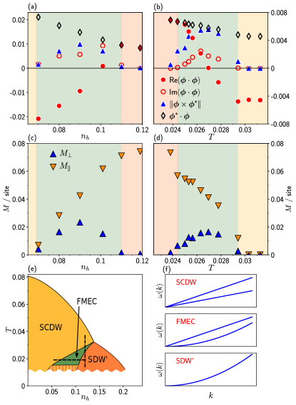
Figure 1: Evolution of the order parameter $\bm{\phi}$ and the net spin moment $\mathbf{M}$ along the constant doping (a,c) and constant temperature (b,d) cuts of the phase diagram (e) of the model with $s$-wave cross-hopping pattern and density-density interaction. (f) A cartoon view of the Nambu-Goldstone modes of the SU(2) symmetric model.

III.1.1 $s$-wave cross-hopping

The $s$-wave cross-hopping is distinguished from the other hopping patterns by a finite and real expectation value of $\phi_{0}\equiv\langle a^{\dagger}_{i\uparrow}b^{\phantom{\dagger}}_{i\downarrow}+a^{\dagger}_{i\uparrow}b^{\phantom{\dagger}}_{i\downarrow}\rangle$. This can be viewed as a spin-singlet component of the exciton condensate generated by a source field present in the Hamiltonian. Exciton condensates with finite singlet and triplet components were shown Volkov and Kopaev (1973); Volkov et al. (1975); Balents (2000); Bascones et al. (2002) to host a ferromagnetic polarization with components $\mathbf{M}_{\perp}\propto i\bm{\phi}^{*}\times\bm{\phi}$, $\mathbf{M}_{\parallel}\propto\phi_{0}^{*}\bm{\phi}+\phi_{0}\bm{\phi}^{*}$. The same spin polarization pattern may be expected here.

In Fig. 1 we show the phase diagram as a function of temperature and hole doping (relative to the half-filling of two electrons per atom) and summarize the evolution of the order parameter $\bm{\phi}$ and of the net spin moment $\mathbf{M}$ along two cuts crossing the SCDW, FMEC and SDW’ phases.

In the SCDW phase $\bm{\phi}=i\mathbf{I}$, implying ${\operatorname{Re}(\bm{\phi}\cdot\bm{\phi})<0}$ and ${\operatorname{Im}(\bm{\phi}\cdot\bm{\phi})=0}$. The net moment ${\mathbf{M}=0}$. The state is time-reversal invariant and thus the continuous spin density vanishes as well. The spin currents present in this state do not give rise to any spin texture, $\mathbf{m}_{\mathbf{k}}=0$ (Fig. 4c-e). In the SU(2) symmetric model (Fig. 4) there are two broken generators of the SU(2) symmetry with vanishing expectation value of their commutator (no net moment). This implies two linear Goldstone modes Watanabe and Murayama (2012).

In the SDW’ phase $\bm{\phi}=\mathbf{R}$, implying ${\operatorname{Re}(\bm{\phi}\cdot\bm{\phi})>0}$, ${\operatorname{Im}(\bm{\phi}\cdot\bm{\phi})=0}$. There is a net spin moment $\mathbf{M}$ parallel to $\mathbf{R}$ ($\mathbf{M}_{\perp}=0$). There is naturally a finite spin texture $\mathbf{m}_{\mathbf{k}}$ parallel to $\mathbf{R}$ (Fig. 6c-e), but no texture in the perpendicular direction. In the SU(2) symmetric case Fig. 6 there are two broken generators of the SU(2) symmetry with finite expectation value of their commutator (the same as in a normal ferromagnet) implying a single quadratic Goldstone mode Watanabe and Murayama (2012).

At low temperatures the transition between the SCDW and SDW’ phase is of the first order. A continuous transition that we find at higher temperatures and study here can possibly proceed via an intermediate polar phase or an FMEC phase. The latter is actually realized. As the transition advances, $\mathbf{R}$ and $\mathbf{I}$ remain approximately perpendicular while changing their magnitudes . In the FMEC phase both $\mathbf{M}_{\parallel}$ and $\mathbf{M}_{\perp}$ are finite and the net magnetization $\mathbf{M}$ lies at a general angle to both $\mathbf{R}$ and $\mathbf{I}$. The spin texture $\mathbf{m}_{\mathbf{k}}$ is found in both directions, parallel and perpendicular to $\mathbf{M}$, but with different structure (Fig. 5c-e). In the SU(2) symmetric case, see Fig. 5, all three generators of the SU(2) symmetry are broken. The finite expectation value of their commutator(s) ($\mathbf{M}$) implies one quadratic and one linear Goldstone mode Watanabe and Murayama (2012).

III.1.2 p,d-wave cross-hopping

In the models with higher-$l$ cross-hopping pattern, the local expectation value $\phi_{0}$ is zero in both the normal and the ordered phases, and polar phases have vanishing ordered moments. In Fig. 2 we show the evolution of $\bm{\phi}$ along a cut in the phase diagram. Note that the SDW and SCDW phases are exchanged relative to the $s$-wave case, due to the opposite sign of $V_{+\nu}V_{-\nu}$ Kuneš and Geffroy (2016); Kuneš and Augustinský (2014).

The SDW phase is characterized by $\bm{\phi}=\mathbf{R}$, implying ${\operatorname{Re}(\bm{\phi}\cdot\bm{\phi})>0}$, ${\operatorname{Im}(\bm{\phi}\cdot\bm{\phi})=0}$. Both $\mathbf{M}$ and $\mathbf{m}_{\mathbf{k}}$ are absent (Fig. 7c-e). There is, however, a local (anti-ferromagnetic) distribution of continuum spin density around each lattice site polarized along $\mathbf{R}$. The Goldstone spectrum consists of two linear modes.

The SCDW’ phase is characterized by $\bm{\phi}=i\mathbf{I}$, implying ${\operatorname{Re}(\bm{\phi}\cdot\bm{\phi})<0}$, ${\operatorname{Im}(\bm{\phi}\cdot\bm{\phi})=0}$. The continuum spin density vanishes everywhere and the state is time-reversal invariant. Unlike the SCDW phase in the $s$-wave case, there is a finite spin texture $\mathbf{m}_{\mathbf{k}}$ with $p$-wave symmetry Kuneš and Geffroy (2016) (Fig. 9c-e), which can be viewed as a $\mathbf{k}$-space anti-ferromagnet. The Goldstone spectrum again consists of two linear modes.

Similar to the $s$-wave case, the transition between the SDW and SCDW’ phases is of first order at low temperatures, and continuous via an intermediate FMEC phase at higher temperatures. Unlike the $s$-wave case, $\mathbf{M}_{\parallel}=0$ and $\operatorname{Im}(\bm{\phi}\cdot\bm{\phi})$=0 along the path. The vectors $\mathbf{M}$, $\mathbf{R}$ and $\mathbf{I}$ thus remain mutually orthogonal along the whole path through the FMEC phase. The transition proceeds by shrinking of $\mathbf{R}$ accompanied by growth of $\mathbf{I}$. There is a $p$-wave spin texture $\mathbf{m}_{\mathbf{k}}$ in the $\mathbf{R}$-$\mathbf{I}$ plane and an $s$-wave texture for perpendicular polarization, Fig. 8c-e. The Goldstone spectrum is the same as in the FMEC phase of the $s$-wave model.

The model with $d$-wave cross-hopping is expected to show a behavior similar to the $p$-wave one, i.e. $\mathbf{M}_{\parallel}=0$ and $\mathbf{R}\perp\mathbf{I}$. The roles of the SDW and SCDW phases are exchanged due to the same sign of $V_{+\nu}V_{-\nu}$ as in the $s$-wave case. The spin texture $\mathbf{m}_{\mathbf{k}}$ exhibits a $d$-wave symmetry in the SDW’ phase. We have not performed a systematic study, but confirmed this conclusion by inspecting a selected point in each of the FMEC and SDW’ phases.

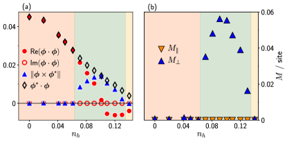
Figure 2: Evolution of the order parameter $\bm{\phi}$ (a) and the net spin moment $\mathbf{M}$ (b) at a constant temperature $T=0.017$ for the model with $p$-wave cross-hopping pattern and density-density interaction Kuneš and Geffroy (2016).

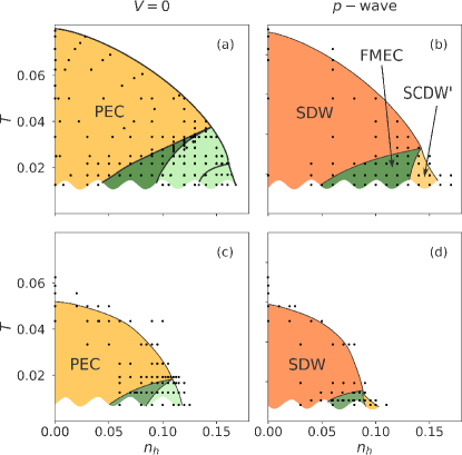
Figure 3: Comparison of models with density-density (a,b) and SU(2) symmetric (c,d) interaction. Panels (a,c) correspond to zero cross-hopping. Panels (b,d) were obtained with a $p$-wave cross-hopping pattern. The dots mark the points for which the calculations were actually performed.

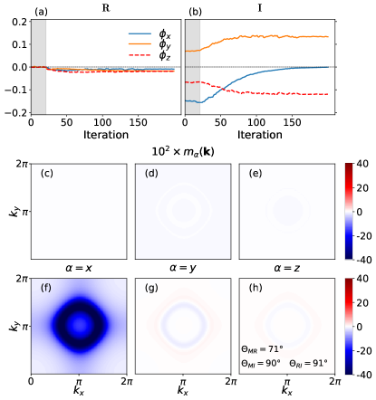
Figure 4: The SCDW phase of the SU(2) symmetric model with $s$-wave cross-hopping with and without an external magnetic field. (a,b) Convergence of the order parameter $\bm{\phi}$. The grey area marks the converged $\mathbf{h}=0$ solution with arbitrary $\bm{\phi}$ orientation. The white area shows the convergence after a field along the $x$-axis is turned on. Panels (c-e) show the spin texture $\mathbf{m}_{\mathbf{k}}$ in the initial $\mathbf{h}=0$ state. Panels (f-h) show $\mathbf{m}_{\mathbf{k}}$ in the converged solution with finite field. In panels (e) and (h) we show the angles $\Theta_{MR}$, $\Theta_{MI}$ and $\Theta_{RI}$ between the vectors $\mathbf{M}$, $\mathbf{R}$ and $\mathbf{I}$ (omitted if corresponding vectors vanish) in zero and finite field, respectively. The calculations were performed for $h_{x}=-0.006$, $n_{h}=0.03$, ${T=0.0125}$, $V=0.04$.

III.1.3 Rotationally invariant interaction

Fig. 3 illustrates the modification of the phase boundaries due to the spin-flip term. Panels (a) and (c) show the $V_{\nu}=0$ case, while panels (b) and (d) correspond to the $p$-wave cross-hopping pattern. The results for the SU(2) symmetric model are qualitatively similar to the density-density case, but the extent of the excitonic phase is reduced. This can be traced back to the higher local degeneracy of the Heisenberg HS state, which favors the normal phase.

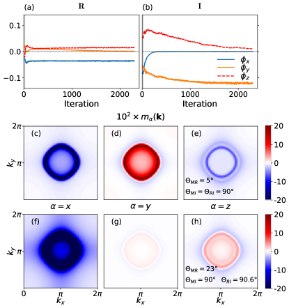
Figure 5: The same as Fig. 4 for the FMEC phase of the SU(2) symmetric model with $s$-wave cross-hopping. The calculations were performed for $h_{x}=-0.006$, $n_{h}=0.07$, $T=0.007$, $V=0.04$. Note that calculations are practically converged after $\sim$800 iterations. The evolution of $\bm{\phi}$ after this point represents mainly rotation around $\mathbf{h}$, i.e., a symmetry transformation of the practically converged solution.

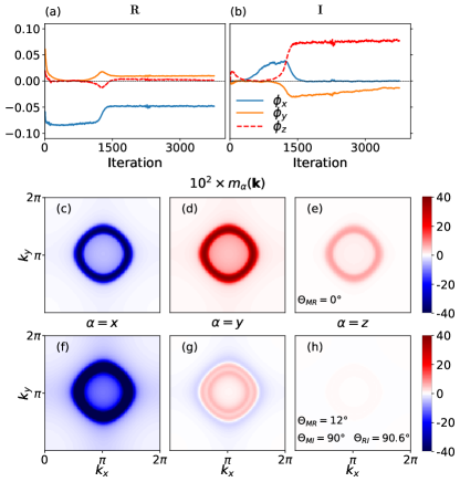
Figure 6: The same as Fig. 4 for the SDW’ phase of the SU(2) symmetric model with $s$-wave cross-hopping. The calculations were performed for $h_{x}=-0.006$, $n_{h}=0.08$, $T=0.0125$, $V=0.04$.

III.2 Spin-triplet condensate in external field

Next, we study the condensate in small magnetic (Zeeman) fields. In particular, we want to investigate the orientation of the order parameter $\bm{\phi}$ with respect to the net moment $\mathbf{M}$ (parallel to the external field). To this end we use the SU(2) symmetric interaction ($\lambda=1$). We start from a converged $\mathbf{h}=0$ result with $\bm{\phi}$ pointing in a general direction. Then a magnetic field $\mathbf{h}$ pointing along the $x$-axis is applied and convergence to the new equilibrium monitored. The field magnitude is chosen to be smaller than the excitonic Weiss field, estimated as the value of the high-frequency limit of the off-diagonal self-energy, but large enough to achieve reasonably fast convergence of the DMFT iterative procedure. For each excitonic phase we show the convergence of $\bm{\phi}$, the spin texture $\mathbf{m}_{\mathbf{k}}$ in zero and finite $\mathbf{h}$ and the angles $\Theta_{MR}$, $\Theta_{MI}$ and $\Theta_{RI}$ between the vectors $\mathbf{M}$, $\mathbf{R}$ and $\mathbf{I}$.

III.2.1 $s$-wave cross-hopping

Starting from a small doping we first visit the SCDW phase, see Fig. 4. As with the density-density interaction at $\mathbf{h}=0$, this phase is characterized by ${\mathbf{R}=\mathbf{M}=\mathbf{m}_{\mathbf{k}}=0}$ and a pattern of local spin currents polarized parallel to $\mathbf{I}$, as discussed in the previous section. The dominant effect of the external field $\mathbf{h}$ is to rotate $\mathbf{I}$ perpendicular to $\mathbf{h}$. This behavior, reminiscent of an antiferromagnet, will be observed also in other cases. A small $\mathbf{R}$ component is induced, which is approximately perpendicular to $\mathbf{h}$ and $\mathbf{I}$.

The FMEC state obtained at higher doping carries a finite net moment $\mathbf{M}$, see Fig.5c-e. The main effect of the external field $\mathbf{h}$ is to align $\mathbf{M}$ along its direction. The finite component of $\mathbf{R}$ perpendicular to $\mathbf{M}$ gives rise to an $s$-wave spin texture that is not parallel to $\mathbf{M}$ and thus integrates to zero over the Brillouin zone, see Fig. 5g-h.

The SDW’ phase also carries a finite spin polarization $\mathbf{M}$, Fig. 6c-e. While a vanishingly small $\mathbf{h}$ would just rotate the ground state to align $\mathbf{M}$ with $\mathbf{h}$, the finite field has a more profound effect. It gives rise to a sizable $\mathbf{I}$ and effectively induces a transition to an FMEC-like state. It is interesting to point out that while in zero field the SDW’ phase has the same uniaxial symmetry as an ordinary ferromagnet, this symmetry is lost in a finite field. It is instructive to inspect the convergence of the iterative procedure, after $\mathbf{h}$ is turned on. First, the system remains in a unstable SDW’-like state ($\mathbf{I}\approx 0$ and $\mathbf{R}\parallel\mathbf{h}$) to eventually settle in an FMEC-like state. Although the convergence does not represent any real dynamics of the system, it suggests the existence of a metastable SDW’-like phase.

III.2.2 $p$-wave cross-hopping

At small doping and $\mathbf{h}=0$ the system is in the SDW phase characterized by ${\mathbf{I}=\mathbf{M}=\mathbf{m}_{\mathbf{k}}=0}$ and finite intra-atomic (collinear antiferromagnetic) spin polarization parallel to $\mathbf{R}$. In the external field $\mathbf{h}$, $\mathbf{R}$ turns perpendicular to $\mathbf{h}$, see Fig. 7. A small $\mathbf{I}$ component perpendicular to $\mathbf{R}$ and $\mathbf{h}$ is induced together with a small net moment.

Applying finite $\mathbf{h}$ in the FMEC phase aligns the spontaneous polarization $\mathbf{M}$ with the external field $\mathbf{h}$ as expected, while the mutual orthogonality of $\mathbf{M}$, $\mathbf{R}$ and $\mathbf{I}$ is preserved. The polarization of the $p$-wave spin texture thus remains perpendicular to $\mathbf{h}$, see Fig. 8.

Finally, the SCDW’ phase at $\mathbf{h}=0$ is invariant with respect to time reversal and thus carries no spin polarization. Nevertheless, the spin-rotational symmetry is broken, as demonstrated by the presence of the spin texture $\mathbf{m}_{\mathbf{k}}$. A finite external field $\mathbf{h}$ generates a state similar to the FMEC case with the spin texture polarized perpendicular to $\mathbf{M}$, see Fig. 9.

In fact, with finite $\mathbf{h}$, all the excitonic phases become equivalent to the FMEC phase, although obvious quantitative differences remain for the case of moderate $\mathbf{h}$ discussed here. We point out that there is still a symmetry difference between the excitonic condensate and the normal state in the presence of finite field, since the condensate does not have the uniaxial symmetry of the normal state.

III.3 Phenomenological model

The above numerical results paint a rather complex picture. In order to understand them we introduce a phenomenological Ginzburg-Landau type (GL) functional, which can be viewed as an extension of the functional of Ref. Kuneš, 2014. We assume that the magnitude of the order parameter $\|\bm{\phi}\|^{2}$ is fixed by the large kinetic energy of excitons and show only the smaller terms that select the direction of $\bm{\phi}$. We start by considering an undoped system. The corresponding GL functional reads

$$E_{0}=\pm\alpha(\mathbf{R}\cdot\mathbf{R}-\mathbf{I}\cdot\mathbf{I})+\beta(\mathbf{R}\times\mathbf{I})\cdot(\mathbf{R}\times\mathbf{I})-\mathbf{h}\cdot(\mathbf{R}\times\mathbf{I}),$$ (9)

with positive constants $\alpha$ and $\beta$. Here the first term describes the effect of cross-hopping on the phase of the order parameter. The plus sign applies to $s$- and $d$-wave cross-hopping, the minus sign to $p$-wave cross-hopping. $\mathbf{R}\times\mathbf{I}=-\tfrac{i}{2}\bm{\phi}^{*}\times\bm{\phi}$ is proportional to the spin polarization of the condensate, so that the second and third terms describe the inter-atomic antiferromagnetic interaction and coupling to the external field, respectively. For $\mathbf{h}=0$, $\beta>0$ implies $\mathbf{R}=0$ for $s$, $d$-wave cross-hopping patterns, and $\mathbf{I}=0$ for the $p$-wave pattern.

The application of a finite external field induces a non-zero complementary component

$$\mathbf{R}=-\frac{\mathbf{h}\times\mathbf{I}}{2[C\pm\alpha+\beta\mathbf{I}\cdot\mathbf{I}]},\quad\mathbf{I}=\frac{\mathbf{h}\times\mathbf{R}}{2[C\mp\alpha+\beta\mathbf{R}\cdot\mathbf{R}]},$$

where $C$ is a Lagrange multiplier fixing $\|\bm{\phi}\|^{2}$. This explains the numerical observation of mutual orthogonality of $\mathbf{h}$, $\mathbf{R}$ and $\mathbf{I}$ in the undoped phases. It also justifies the use of the density-density approximation with the field applied along the $z$-axis, i.e. perpendicular to the condensate Kuneš and Augustinský (2014).

Doping introduces additional terms to the functional. To proceed we start from the generalized double-exchange model Kuneš and Geffroy (2016); Chaloupka and Khaliullin (2016). We introduce terms that describe the polarization of the doped carriers and its coupling to the condensate

$$E=E_{0}+\gamma\mathbf{\widetilde{M}}\cdot(\mathbf{R}\times\mathbf{I})-\mathbf{h}\cdot\mathbf{\widetilde{M}}+\delta\mathbf{\widetilde{M}}\cdot\mathbf{R}+\omega\mathbf{\widetilde{M}}\cdot\mathbf{\widetilde{M}},$$ (10)

where $\mathbf{\widetilde{M}}$ stands for the spin polarization of the doped carriers. The second term describes the standard double-exchange interaction between the local moments of the condensate and the itinerant carriers. The third and fifth terms ($\omega>0$) describe the polarizability of the doped carriers. The fourth term describes the coupling between the condensate and the doped carriers due to the finite cross-hopping. This term has a more complicated $\mathbf{k}$-dependent form Kuneš and Geffroy (2016), but to discuss the response to a uniform field we keep only the part containing $\mathbf{\widetilde{M}}$. The key observation is that $\delta\neq 0$ for $s$-wave cross-hopping, while $\delta=0$ for $p$- and $d$-wave cross-hopping.

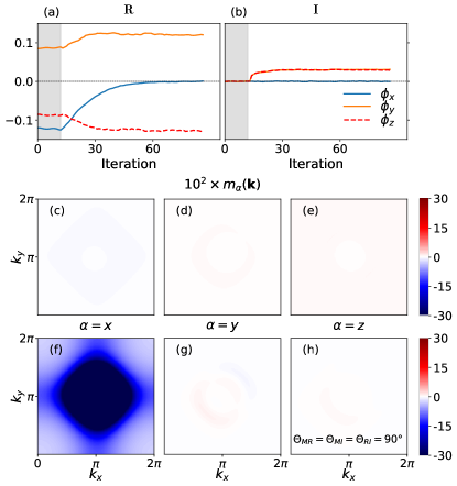
Figure 7: The same as Fig. 4 for the SDW phase of the SU(2) symmetric model with $p$-wave cross-hopping. The calculations were performed for ${h_{x}=-0.01}$, ${n_{h}=0.03}$, ${T=0.033}$, ${V=0.04}$.

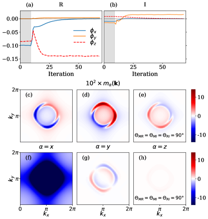
Figure 8: The same as Fig. 4 for the FMEC phase of the SU(2) symmetric model with $p$-wave cross-hopping. The calculations were performed for ${h_{x}=-0.01}$, ${n_{h}=0.6}$, ${T=0.007}$, ${V=0.04}$.

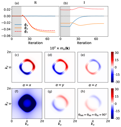
Figure 9: The same as Fig. 4 for the SCDW’ phase of the SU(2) symmetric model with $p$-wave cross-hopping. The calculations were performed for $h_{x}=-0.01$, $n_{h}=0.095$, ${T=0.007}$, $V=0.04$.

The stationary values of $\mathbf{R}$, $\mathbf{I}$ and $\mathbf{\widetilde{M}}$ satisfy

$$\begin{split}&\mathbf{R}=\frac{\mathbf{I}\times(\mathbf{h}-\gamma\mathbf{\widetilde{M}})-\delta\mathbf{\widetilde{M}}}{2[C\pm\alpha+\beta\mathbf{I}\cdot\mathbf{I}]},\quad\mathbf{I}=\frac{\mathbf{R}\times(\gamma\mathbf{\widetilde{M}}-\mathbf{h})}{2[C\mp\alpha+\beta\mathbf{R}\cdot\mathbf{R}]}\\ &\mathbf{\widetilde{M}}=\frac{1}{2\omega}(\mathbf{h}-\gamma\mathbf{R}\times\mathbf{I}-\delta\mathbf{R}).\end{split}$$

This implies the orthogonality of $\mathbf{I}$ to $\mathbf{\widetilde{M}}$, $\mathbf{h}$ and $\mathbf{R}$, as observed in the numerical calculations. For $p$- and $d$-wave cross-hopping, $\delta=0$ so that $\mathbf{R}$ is orthogonal to $\mathbf{h}$ and $\mathbf{\widetilde{M}}$ (which are parallel in this case) as well. Finite $\delta$ in the $s$-wave case leads to a general angle between the coplanar vectors $\mathbf{R}$, $\mathbf{\widetilde{M}}$ and $\mathbf{h}$. This behavior of the $s$-wave model reproduces the numerical results only approximately. While $\mathbf{I}\cdot\mathbf{h}=0$ is fulfilled to our numerical accuracy, we find small, but non-negligible, deviations from $\mathbf{I}\cdot\mathbf{R}=0$, which must be due to effects beyond Eq. 10.

III.4 Spontaneous spin current

The spin texture with $\mathbf{m}_{-\mathbf{k}}=-\mathbf{m}_{\mathbf{k}}$ in the SCDW’ and FMEC phases for $p$-wave cross-hopping, Figs. 8-9, may suggest that electrons moving in opposite directions carry opposite spin polarization. Things are not so simple, since the current (8) depends on the group velocities, which have opposite signs for $a$ and $b$ orbitals of the present model.

The calculated spin currents (8) in the phases with $p$-wave spin texture, marked by points in Fig. 3, are shown in Fig. 10. We find a finite net spin current polarized along, and scaling with $\mathbf{I}$ . This shows that DMFT violates the so-called Bloch theorem Brillouin (1933); Ohashi and Momoi (1996), which forbids spontaneous currents of charges that are locally conserved by the interaction Hamiltonian. In the Appendix B we sketch the proof for the present model at $T=0$. A general proof for finite temperatures can be found in Ref. Ohashi and Momoi, 1996.

Comparing Eq. 8 with the definition of the spin texture $\mathbf{m}_{\mathbf{k}}$, it is clear that a vanishing of spin current does not require that $\mathbf{m}_{\mathbf{k}}=0$. We assume that a spin texture exists also in the exact ground state of the model, while the spin current is suppressed by the momentum-dependence of the self-energy, absent in DMFT. If so, a finite spin current may be obtained by breaking the balance between the orbital contributions to (8) in a non-equilibrium state generated by an optical excitation.

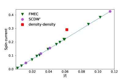
Figure 10: Magnitude of the spin current versus amplitude of the imaginary part of the order parameter, in two distinct phases using the SU(2) symmetric interaction (green triangles and magenta circles for FMEC and SCDW’, respectively), and the density-density approximation (red square). The dashed line is a guide for the eye.

IV Conclusions

We have studied the influence of an external magnetic field on the excitonic condensate in the two-band Hubbard model. In all studied phases the excitonic condensate breaks the uniaxial symmetry imposed by the external field and the excitonic condensation thus remains a thermodynamic phase transition accompanied by the appearance of gapless Goldstone modes.

There is a ubiquitous $\mathbf{h}\cdot(\mathbf{R}\times\mathbf{I})$ coupling between the field and condensate, which generates perpendicular (to $\mathbf{h}$) components of the order parameter $\bm{\phi}$. As a result the staggered spin density or spin current density polarization in the model with $p$- and $d$-wave cross-hooping lie perpendicular to the external field, analogous to the behavior of an Heisenberg antiferromagnet. For $s$-wave cross-hopping, an additional linear coupling $\mathbf{h}\cdot\mathbf{R}$ exists giving rise to a more complicated behavior.

Finally, we have observed that a net spin current is spontaneously generated in some excitonic phases with $p$-wave cross-hopping. We attribute the violation of Bloch’s no-go theorem to the local self-energy approximation of the dynamical mean-field theory. We propose that a net non-equilibrium spin or charge current may be generated by a uniform orbital or spin-orbital selective excitation in phase with the $p$-wave spin texture.

Appendix A Expression for the spin current

We consider the model Hamiltonian (2). The local charge and spin operators read

$$n_{\mathbf{i}}= s^{0}_{\mathbf{i}}=\sum_{\sigma}\left(a_{\mathbf{i}\sigma}^{\dagger}a^{\phantom{\dagger}}_{\mathbf{i}\sigma}+b_{\mathbf{i}\sigma}^{\dagger}b^{\phantom{\dagger}}_{\mathbf{i}\sigma}\right)$$ (11)

$$s^{\gamma}_{\mathbf{i}}= \sum_{\alpha,\beta}\sigma^{\gamma}_{\alpha\beta}\left(a_{\mathbf{i}\alpha}^{\dagger}a^{\phantom{\dagger}}_{\mathbf{i}\beta}+b_{\mathbf{i}\alpha}^{\dagger}b^{\phantom{\dagger}}_{\mathbf{i}\beta}\right),$$

where $\sigma^{\gamma}$ ($\gamma=0,x,y,z$) are the Pauli matrices. The density operator commutes with the local part of the Hamiltonian

$$[n_{\mathbf{i}},H_{\text{loc}}]=[s^{z}_{\mathbf{i}},H_{\text{loc}}]=0.\\$$ (12)

For the SU(2) symmetric interaction, all the components of the local spin operator commute with $H_{\text{loc}}$

$$[s^{\gamma}_{\mathbf{i}},H_{\text{loc}}]=0\quad\text{if}\quad\lambda=1\\$$ (13)

We can define the current using the continuity equation, which takes the form of Kirchhoff’s first law

$$\partial_{t}s^{\gamma}_{\mathbf{i}}=\sum_{\nu}\left(j^{\gamma}_{\mathbf{i}-\mathbf{e}_{\nu}\nu}-j^{\gamma}_{\mathbf{i}\nu}\right),$$ (14)

where $j^{\gamma}_{\mathbf{i}\nu}$ is the current flowing on the bond $\mathbf{i}\rightarrow\mathbf{i}+\mathbf{e}_{\nu}$. The time derivative of the local density operator can be evaluated using the equation of motion

$$\partial_{t}s^{\gamma}_{\mathbf{i}}=i[H,s^{\gamma}_{\mathbf{i}}]=i\sum_{\nu}[T_{\nu}+T_{\nu}^{\dagger},s^{\gamma}_{\mathbf{i}}].$$ (15)

We distinguish between the ’right’- and the ’left’-hopping parts ($T$ and $T^{\dagger}$ respectively) of the kinetic energy for future convenience. For the right-hopping part, we find

$$\begin{split}&i[T_{\nu},s^{\gamma}_{\mathbf{i}}]\\ =&it_{a}\sum_{\alpha,\beta}\sigma^{\gamma}_{\alpha\beta}\left(a_{\mathbf{i}+\mathbf{e}_{\nu}\alpha}^{\dagger}a^{\phantom{\dagger}}_{\mathbf{i}\beta}-a_{\mathbf{i}\alpha}^{\dagger}a^{\phantom{\dagger}}_{\mathbf{i}-\mathbf{e}_{\nu}\beta}\right)\\ +&it_{b}\sum_{\alpha,\beta}\sigma^{\gamma}_{\alpha\beta}\left(b_{\mathbf{i}+\mathbf{e}_{\nu}\alpha}^{\dagger}b^{\phantom{\dagger}}_{\mathbf{i}\beta}-b_{\mathbf{i}\alpha}^{\dagger}b^{\phantom{\dagger}}_{\mathbf{i}-\mathbf{e}_{\nu}\beta}\right)\\ +&iV_{+\nu}\sum_{\alpha,\beta}\sigma^{\gamma}_{\alpha\beta}\left(a_{\mathbf{i}+\mathbf{e}_{\nu}\alpha}^{\dagger}b^{\phantom{\dagger}}_{\mathbf{i}\beta}-a_{\mathbf{i}\alpha}^{\dagger}b^{\phantom{\dagger}}_{\mathbf{i}-\mathbf{e}_{\nu}\beta}\right)\\ +&iV_{-\nu}\sum_{\alpha,\beta}\sigma^{\gamma}_{\alpha\beta}\left(b_{\mathbf{i}+\mathbf{e}_{\nu}\alpha}^{\dagger}a^{\phantom{\dagger}}_{\mathbf{i}\beta}-b_{\mathbf{i}\alpha}^{\dagger}a^{\phantom{\dagger}}_{\mathbf{i}-\mathbf{e}_{\nu}\beta}\right).\end{split}$$ (16)

The operator $s^{\gamma}_{\mathbf{i}}$ is Hermitian, therefore

$$[T_{\nu}^{\dagger},s^{\gamma}_{\mathbf{i}}]=-[T_{\nu},s^{\gamma}_{\mathbf{i}}]^{\dagger}.$$ (17)

Combining Eqs. 14, 16 and 17, we get

$$\begin{split}j^{\gamma}_{\mathbf{i}\nu}=&-\sum_{\alpha,\beta}\left(it_{a}\sigma^{\gamma}_{\alpha\beta}a_{\mathbf{i}+\mathbf{e}_{\nu}\alpha}^{\dagger}a^{\phantom{\dagger}}_{\mathbf{i}\beta}+\text{H.c.}\right)\\ &-\sum_{\alpha,\beta}\left(it_{b}\sigma^{\gamma}_{\alpha\beta}b_{\mathbf{i}+\mathbf{e}_{\nu}\alpha}^{\dagger}b^{\phantom{\dagger}}_{\mathbf{i}\beta}+\text{H.c.}\right)\\ &-\sum_{\alpha,\beta}\left(iV_{+\nu}\sigma^{\gamma}_{\alpha\beta}a_{\mathbf{i}+\mathbf{e}_{\nu}\alpha}^{\dagger}b^{\phantom{\dagger}}_{\mathbf{i}\beta}+\text{H.c.}\right)\\ &-\sum_{\alpha,\beta}\left(iV_{-\nu}\sigma^{\gamma}_{\alpha\beta}b_{\mathbf{i}+\mathbf{e}_{\nu}\alpha}^{\dagger}a^{\phantom{\dagger}}_{\mathbf{i}\beta}+\text{H.c.}\right).\end{split}$$ (18)

The global current is defined as the sum over all bonds/sites

$$J^{\gamma}_{\nu}\equiv\sum_{\mathbf{i}}j^{\gamma}_{\mathbf{i}\nu}.$$ (19)

Appendix B Extension of a result by Brillouin

In this section, we show that a state that carries a finite current of locally conserved density cannot be a ground state. We follow the proof in Ref. Ohashi and Momoi, 1996. Let us assume that $|\Psi\rangle$ is a ground state, which has a finite expectation value of global current $\langle\Psi|J^{\gamma}_{x}|\Psi\rangle=J\neq 0$, and construct a state

$$\ket{\Phi}\equiv\exp(-i\delta X^{\gamma})\ket{\Psi},$$ (20)

where

$$X^{\gamma}\equiv\sum_{k,l}ks^{\gamma}_{(k,l)}.$$ (21)

Since $X^{\gamma}$ commutes with $H_{\text{loc}}$ we get

$$\begin{split}\matrixelement{\Phi}{H}{\Phi}&=\matrixelement{\Psi}{H_{\text{loc}}}{\Psi}+\\ \sum_{\nu}&\matrixelement{\Psi}{\exp(i\delta X^{\gamma})(T_{\nu}+T_{\nu}^{\dagger})\exp(-i\delta X^{\gamma})}{\Psi}.\end{split}$$ (22)

The operators $X^{\gamma}$ and $T_{\nu}+T_{\nu}^{\dagger}$ are Hermitian, we can thus expand (22) using the Baker-Hausdorff lemma

$$\begin{split}&\exp(i\delta B)A\exp(-i\delta B)=A+i\delta[B,A]+\\ &\frac{(i\delta)^{2}}{2!}[B,[B,A]]+\dots\frac{(i\delta)^{n}}{n!}[B,[B,\ldots,[B,A]\ldots]]\ldots\end{split}$$ (23)

To compute $[X^{\gamma},T_{\nu}]$ we use Eq. 16 and obtain

$$[X^{\gamma}, T_{y}]=0,$$ (24)

$$[X^{\gamma}, T_{x}]=-\sum_{k,l}k[T_{x},s^{\gamma}_{(k,l)}]$$

$$= -\sum_{\alpha\beta}\sigma^{\gamma}_{\alpha\beta}\sum_{k,l}\left(k-(k+1)\right)$$

$$\times\biggl{[} t_{a}a_{(k+1,l)\alpha}^{\dagger}a^{\phantom{\dagger}}_{(k,l)\beta}\biggr{.}\biggl{.}+t_{b}b_{(k+1,l)\alpha}^{\dagger}b^{\phantom{\dagger}}_{(k,l)\beta}\biggr{.}$$

. $$V_{x}a_{(k+1,l)\alpha}^{\dagger}b^{\phantom{\dagger}}_{(k,l)\beta}+V_{-x}b_{(k+1,l)\alpha}^{\dagger}a^{\phantom{\dagger}}_{(k,l)\beta}\biggr{]}$$

$$=\sum_{\mathbf{i}}\sum_{\alpha\beta}\sigma^{\gamma}_{\alpha\beta}\biggl{[} t_{a}a_{\mathbf{i}+\mathbf{e}_{x}\alpha}^{\dagger}a^{\phantom{\dagger}}_{\mathbf{i}\beta}+t_{b}b_{\mathbf{i}+\mathbf{e}_{x}\alpha}^{\dagger}b^{\phantom{\dagger}}_{\mathbf{i}\beta}\biggr{.}$$

$$\biggl{.}+ V_{x}a_{\mathbf{i}+\mathbf{e}_{x}\alpha}^{\dagger}b^{\phantom{\dagger}}_{\mathbf{i}\beta}+V_{-x}b_{\mathbf{i}+\mathbf{e}_{x}\alpha}^{\dagger}a^{\phantom{\dagger}}_{\mathbf{i}\beta}\biggr{]}.$$

Using the identity $[X^{\gamma},T^{\dagger}]=-[X^{\gamma},T]^{\dagger}$ we arrive at

$$\begin{split}&[X^{\gamma},T_{x}+T_{x}^{\dagger}]=iJ_{x}^{\gamma}.\end{split}$$ (25)

We can also evaluate the next commutator

$$[X^{\gamma},[X^{\gamma},T_{x}+T_{x}^{\dagger}]]=[X^{\gamma},iJ_{x}^{\gamma}]$$

$$=\sum_{k,l} \quantity(k+1-k)$$

$$\times\sum_{\alpha} \left[t_{a}a_{(k+1,l)\alpha}^{\dagger}a^{\phantom{\dagger}}_{(k,l)\alpha}+t_{b}b_{(k+1,l)\alpha}^{\dagger}b^{\phantom{\dagger}}_{(k,l)\alpha}\right.$$

$$\left.+V_{x}a_{(k+1,l)\alpha}^{\dagger}b^{\phantom{\dagger}}_{(k,l)\alpha}+V_{-x}b_{(k+1,l)\alpha}^{\dagger}a^{\phantom{\dagger}}_{(k,l)\alpha}\right]$$

$$+H.c.$$

$$=T_{x} +T_{x}^{\dagger}.$$ (26)

We finally obtain

$$\begin{split}\matrixelement{\Phi}{H}{\Phi}&=\matrixelement{\Psi}{H}{\Psi}-\sin\delta\matrixelement{\Psi}{J_{x}^{\gamma}}{\Psi}\\ &+(\cos\delta-1)\matrixelement{\Psi}{T_{x}+T_{x}^{\dagger}}{\Psi}\\ &=\langle\Psi|H|\Psi\rangle-\delta J+\mathcal{O}(\delta^{2}).\end{split}$$ (27)

Therefore $\ket{\Psi}$ cannot be a ground state if $J$ is finite.

References

- Mott (1961) N. F. Mott, Philos. Mag. 6, 287 (1961).
- Knox (1963) R. S. Knox, Solid State Phys. Suppl. 5, 100 (1963).
- Keldysh and Kopaev (1965) L. V. Keldysh and Y. V. Kopaev, Sov. Phys. Solid State 6, 2219 (1965).
- des Cloizeaux (1965) J. des Cloizeaux, J. Phys. Chem. Solids 26, 259 (1965).
- Halperin and Rice (1968a) B. I. Halperin and T. M. Rice, “Solid state physics,” (Academic Press, New York, 1968) p. 115.
- Jain et al. (2017) A. Jain, M. Krautloher, J. Porras, G. H. Ryu, D. P. Chen, D. L. Abernathy, J. T. Park, A. Ivanov, J. Chaloupka, G. Khaliullin, B. Keimer, and B. J. Kim, Nat. Phys. 13, 633 (2017).
- Eisenstein and MacDonald (2004) J. P. Eisenstein and A. H. MacDonald, Nature 432, 691 (2004).
- Balents (2000) L. Balents, Phys. Rev. B 62, 2346 (2000).
- Kuneš (2014) J. Kuneš, Phys. Rev. B 90, 235140 (2014).
- Khaliullin (2013) G. Khaliullin, Phys. Rev. Lett. 111, 197201 (2013).
- Kaneko and Ohta (2014) T. Kaneko and Y. Ohta, Phys. Rev. B 90, 245144 (2014).
- Kaneko et al. (2015) T. Kaneko, B. Zenker, H. Fehske, and Y. Ohta, Phys. Rev. B 92, 115106 (2015).
- Tatsuno et al. (2016) T. Tatsuno, E. Mizoguchi, J. Nasu, M. Naka, and S. Ishihara, J. Phys. Soc. Japan 85, 83706 (2016).
- Nasu et al. (2016) J. Nasu, T. Watanabe, M. Naka, and S. Ishihara, Phys. Rev. B 93, 205136 (2016).
- Kuneš and Geffroy (2016) J. Kuneš and D. Geffroy, Phys. Rev. Lett. 116, 256403 (2016).
- Kuneš and Augustinský (2014) J. Kuneš and P. Augustinský, Phys. Rev. B 90, 235112 (2014).
- Yamaguchi et al. (2017) T. Yamaguchi, K. Sugimoto, and Y. Ohta, J. Phys. Soc. Japan 86, 043701 (2017).
- Afonso and Kuneš (2017) J. F. Afonso and J. Kuneš, Phys. Rev. B 95, 115131 (2017).
- Wadley et al. (2016) P. Wadley, B. Howells, J. Železný, C. Andrews, V. Hills, R. P. Campion, V. Novák, K. Olejník, F. Maccherozzi, S. S. Dhesi, S. Y. Martin, T. Wagner, J. Wunderlich, F. Freimuth, Y. Mokrousov, J. Kuneš, J. S. Chauhan, M. J. Grzybowski, A. W. Rushforth, K. Edmond, B. L. Gallagher, and T. Jungwirth, Science 351, 587 (2016).
- Wu et al. (2007) C. Wu, K. Sun, E. Fradkin, and S.-C. Zhang, Phys. Rev. B 75, 115103 (2007).
- Brillouin (1933) L. Brillouin, J. Phys. Radium 4, 333 (1933).
- Smith and Wilhelm (1935) H. G. Smith and J. O. Wilhelm, Rev. Mod. Phys. 7, 237 (1935).
- Bohm (1949) D. Bohm, Phys. Rev. 75, 502 (1949).
- Volkov and Kopaev (1978) B. A. Volkov and Y. Kopaev, JETP LETT. 27, 7 (1978).
- Volkov et al. (1981) B. A. Volkov, A. A. Gorbatsevich, Y. Kopaev, and V. Tugushev, Sov. Phys. JETP 54, 1008 (1981).
- Gorbatsevich et al. (1983) A. Gorbatsevich, Y. Kopaev, and V. Tugushev, Zh. Eksp. Teor. Fiz , 1107 (1983).
- Tugushev (1984) V. Tugushev, Zh. Eksp. Teor. Fiz. 86, 1282 (1984).
- Ohashi and Momoi (1996) Y. Ohashi and T. Momoi, J. Phys. Soc. Japan 65, 3254 (1996).
- Jung et al. (2015) J. Jung, M. Polini, and A. H. MacDonald, Phys. Rev. B 91, 155423 (2015).
- Mironov and Buzdin (2017) S. Mironov and A. Buzdin, Phys. Rev. Lett. 118, 077001 (2017).
- Werner and Millis (2007) P. Werner and A. J. Millis, Phys. Rev. Lett. 99, 126405 (2007).
- Kuneš and Augustinský (2014) J. Kuneš and P. Augustinský, Phys. Rev. B 89, 115134 (2014).
- Georges et al. (1996) A. Georges, G. Kotliar, W. Krauth, and M. Rozenberg, Rev. Mod. Phys. 68, 13 (1996).
- Werner et al. (2006) P. Werner, A. Comanac, L. de’ Medici, M. Troyer, and A. J. Millis, Phys. Rev. Lett. 97, 076405 (2006).
- Ho (1998) T.-L. Ho, Phys. Rev. Lett. 81, 742 (1998).
- Vollhardt and Woelfle (1990) D. Vollhardt and P. Woelfle, The Superfluid Phases Of Helium 3 (Taylor & Francis, 1990).
- Halperin and Rice (1968b) B. I. Halperin and T. M. Rice, Rev. Mod. Phys. 40, 755 (1968b).
- Kuneš (2015) J. Kuneš, J. Phys. Condens. Matter 27, 333201 (2015).
- Hoshino and Werner (2016) S. Hoshino and P. Werner, Phys. Rev. B 93, 155161 (2016).
- Hariki et al. (2015) A. Hariki, A. Yamanaka, and T. Uozumi, J. Phys. Soc. Jpn. 84, 073706 (2015).
- Volkov and Kopaev (1973) B. A. Volkov and Y. V. Kopaev, JETP Lett. 19, 104 (1973).
- Volkov et al. (1975) B. A. Volkov, Y. V. Kopaev, and A. I. Rusinov, Sov. Phys. JETP 41, 952 (1975).
- Bascones et al. (2002) E. Bascones, A. A. Burkov, and A. H. MacDonald, Phys. Rev. Lett. 89, 086401 (2002).
- Watanabe and Murayama (2012) H. Watanabe and H. Murayama, Phys. Rev. Lett. 108, 251602 (2012).
- Chaloupka and Khaliullin (2016) J. Chaloupka and G. Khaliullin, Phys. Rev. Lett. 116, 017203 (2016).