xGASS: Total cold gas scaling relations and molecular-to- atomic gas ratios of galaxies in the local Universe

Abstract

We present the extended GALEX Arecibo SDSS Survey (xGASS), a gas fraction-limited census of the atomic hydrogen (Hi) gas content of 1179 galaxies selected only by stellar mass ($M_{\star}$$=10^{9}-10^{11.5}$ M_⊙) and redshift ($0.01<z<0.05$). This includes new Arecibo observations of 208 galaxies, for which we release catalogs and Hi spectra. In addition to extending the GASS Hi scaling relations by one decade in stellar mass, we quantify total (atomic+molecular) cold gas fractions and molecular-to-atomic gas mass ratios, $R_{\rm mol}$, for the subset of 477 galaxies observed with the IRAM 30 m telescope. We find that atomic gas fractions keep increasing with decreasing stellar mass, with no sign of a plateau down to $\log M_{\star}/M_{\odot}=9$. Total gas reservoirs remain Hi-dominated across our full stellar mass range, hence total gas fraction scaling relations closely resemble atomic ones, but with a scatter that strongly correlates with $R_{\rm mol}$, especially at fixed specific star formation rate. On average, $R_{\rm mol}$ weakly increases with stellar mass and stellar surface density $\mu_{\star}$, but individual values vary by almost two orders of magnitude at fixed $M_{\star}$ or $\mu_{\star}$. We show that, for galaxies on the star-forming sequence, variations of $R_{\rm mol}$ are mostly driven by changes of the Hi reservoirs, with a clear dependence on $\mu_{\star}$. Establishing if galaxy mass or structure plays the most important role in regulating the cold gas content of galaxies requires an accurate separation of bulge and disk components for the study of gas scaling relations.

1 Introduction

The gas-star formation cycle is central to the formation and evolution of galaxies (see e.g. Leroy et al. 2008; Lilly et al. 2013 and review by Kennicutt & Evans 2012). Understanding the complex interplay between the various components (such as multi-phase neutral and ionised gas, and dust) of the interstellar medium (ISM; McKee & Ostriker 1977; Cox 2005) and star formation as a function of galaxy properties, environment and cosmic time is a formidable task, which requires sensitive measurements across the electromagnetic spectrum and on multiple spatial scales for statistical data sets, as well as detailed numerical simulations to gain insights into the physical processes involved.

Even when we restrict ourselves to the global properties of galaxies in the local Universe, gathering the necessary data remains challenging. The main limitation comes from the paucity of measurements of the cold gas content for large, representative galaxy samples compared to optical, infrared, or ultraviolet surveys. Blind surveys of atomic hydrogen such as the Hi Parkes All-Sky Survey (Barnes et al., 2001; Meyer et al., 2004; Wong et al., 2006), and the Arecibo Legacy Fast ALFA survey (ALFALFA; Giovanelli et al., 2005; Haynes et al., 2011) measured the Hi content for $\sim$50,000 galaxies, but detect only the most gas-rich systems in most of their volume ($\sim$7000 deg² and $z<0.06$ for ALFALFA). Samples of molecular hydrogen content, which is traced by carbon monoxide (¹²CO, hereafter CO) line emission, are almost two orders of magnitude smaller (Young et al., 1995; Saintonge et al., 2011; Boselli, Cortese & Boquien, 2014; Bothwell et al., 2014; Cicone et al., 2017). As a result, accurate constraints for key parameters such as the molecular-to-atomic gas mass ratio as a function of galaxy properties for unbiased samples are still scarce.

It is indeed generally accepted that atomic hydrogen has to transition into molecular phase in order to fuel star formation (Blitz & Rosolowsky, 2006; Bigiel et al., 2008; Leroy et al., 2008; Krumholz, McKee & Tumlinson, 2009), although molecular gas could just be tracing star formation, formed as the by-product of the gravitational collapse of atomic gas (Glover & Clark, 2012). The partition of total cold gas into Hi and H₂ and the efficiency of the atomic-to-molecular conversion are thus crucial quantities to measure in order to determine the physical processes regulating the star formation cycle in galaxies.

Substantial observing effort in the past decade went into measuring atomic and molecular gas masses for large samples of galaxies selected from optical surveys, and largely missed by Hi-blind surveys (e.g., Serra et al., 2012; Young et al., 2011; Boselli, Cortese & Boquien, 2014).

Our GALEX Arecibo SDSS Survey (GASS; Catinella et al., 2010) was designed to investigate the main gas fraction scaling relations for a representative (in terms of Hi content), stellar mass-selected sample of galaxies with stellar masses greater than $10^{10}$ M_⊙. The gas fraction limited nature of our observations means that integration times on each source were dictated by the request to reach gas fraction limits of $\sim$2%, thus providing the most sensitive Hi measurements for a large sample currently available. The combination of GASS on Arecibo and its follow-up program on the IRAM 30m telescope (COLD GASS survey, Saintonge et al., 2011) resulted in a benchmark multi-wavelength data set, including physical information about the stars and both atomic and molecular hydrogen gas phases in massive systems.

There were very good reasons to extend GASS and COLD GASS down to a stellar mass of $10^{9}$ M_⊙. First, these extensions would allow us to probe a crucial “sweet spot” for understanding the physical processes that regulate the conversion of gas into stars and shape star-forming galaxies, without the additional complexities introduced by the presence of massive bulges and active galactic nuclei that are ubiquitous in the GASS stellar mass regime. Second, the scatter in the gas fraction scaling relations is expected to be driven by intrinsic properties of the disks, such as amount of angular momentum and stellar surface density (e.g., Fu et al., 2010). Again, testing this prediction with GASS is hampered by the presence of massive bulges, which could influence gas content as well (e.g., Martig et al., 2009). The new observations target a stellar mass regime that is dominated by star-forming disks, thus greatly alleviating these limitations. As showed by GASS, examining the scatter around the mean relations, and particularly its second-parameter dependencies, requires statistical samples of several hundred galaxies.

Here we present the complete low-mass extension of GASS, hereafter GASS-low, which includes new Arecibo observations of 208 galaxies. The combination of GASS and GASS-low, which we refer to as the extended GASS (xGASS) survey, results in a representative sample of 1179 galaxies covering the $9<$ log $M_{\star}$/M_⊙$<11.5$ stellar mass interval (see Section 2.2).

The companion extension of the molecular gas survey, COLD GASS-low, and the properties of the full xCOLD GASS sample are presented in Saintonge et al. (2017). Unlike the original GASS and COLD GASS surveys that were designed to explore the transition between star-forming and passive galaxies, these low-mass extensions aim to understand the basic physical processes governing star-forming galaxies.

This paper is organized as follows. In Section 2 we describe the sample selection and Arecibo observations of GASS-low galaxies, and combine these with GASS to obtain the xGASS representative sample. This includes the correct proportion of Hi-rich ALFALFA galaxies that were not targeted to increase survey efficiency, and thus is representative of the Hi properties of the galaxy population in our stellar mass and redshift intervals. We summarize in Section 3 the main properties of the xCOLD GASS survey, and discuss the overlap sample with both Hi and H₂ observations. Our Hi, total gas, and H₂/Hi scaling relations are presented in Section 4; model comparisons are discussed in Section 5. We summarize our main findings and conclude in Section 6. The GASS-low data release can be found in Appendix A.

All the distance-dependent quantities in this work are computed assuming a cosmology with $H_{0}=70$ km s^-1 Mpc^-1, $\Omega_{m}=0.3$ and $\Omega_{\lambda}=0.7$. We assume a Chabrier (2003) initial mass function. AB magnitudes are used throughout the paper.

2 xGASS: the extended GASS survey

2.1 The low-mass extension of GASS

2.1.1 Sample selection and survey strategy

The galaxies of the GASS low-mass extension were selected from a parent sample of 872 sources extracted from the intersection of the SDSS DR7 (Abazajian et al., 2009) spectroscopic survey, the GALEX Medium Imaging Survey (Martin et al., 2005) and projected ALFALFA footprints according to the following criteria:

• Stellar mass $9.0<{\rm log}M_{\star}/M_{\odot}<10.2$

• Redshift $0.01<z<0.02$.

Because GASS-low targets smaller galaxies than GASS, we lowered the redshift interval to ease their detection (GASS was limited to $0.025<z<0.05$). Galaxies in these stellar mass and redshift intervals have angular diameters smaller than 1 arcmin (as in GASS). Thus our targets fit comfortably within a single SDSS frame and GALEX pointing, so that accurate photometry (and hence stellar masses and star formation rates) can be measured, and a single pointing of the IRAM 30m telescope recovers an accurate total CO flux in most cases.

For GASS, we imposed a flat stellar mass distribution for our targets, in order to ensure enough statistics at the high-mass end. Similarly, we sampled the stellar mass interval of GASS-low galaxies roughly evenly (see Section 2.2.1).

In order to optimize survey efficiency, we prioritized the observations of the galaxies lying within the ALFALFA 40% (hereafter AA40; Haynes et al., 2011) footprint and/or galaxies already observed with the IRAM telescope. Galaxies with good quality Hi detections already available from AA40 or the Cornell Hi digital archive (Springob et al., 2005, hereafter S05) were not reobserved (see Section 2.2 below).

Following the GASS strategy, we observed the targets until detected, or until a limit of a few percent in gas mass fraction ($M_{\rm HI}$/$M_{\star}$) was reached. Practically, we set a limit of $M_{\rm HI}/M_{\star}>0.02$ for galaxies with ${\rm log}(M_{\star}/M_{\odot})>9.7$, and a constant gas mass limit ${\rm log}(M_{\rm HI}/M_{\odot})=8$ for galaxies with smaller stellar masses. This corresponds to a gas fraction limit of $0.02-0.1$ for the whole sample.

Given the Hi mass limit assigned to each galaxy (set by its gas fraction limit and stellar mass), we computed the on-source observing time, $T_{\rm max}$, required to reach that value with our observing mode and instrumental setup, assuming a velocity width of 200 km s^-1, smoothing to half width, and signal-to-noise of 5. The $T_{\rm max}$ values thus obtained vary between 1 and 95 minutes.

2.1.2 Arecibo observations and data reduction

GASS-low observations started in August 2012 and ended in May 2015. These were scheduled in 100 observing runs under Arecibo programs A2703 and A2749; the total telescope time allocation was 263 hours.

The observing mode and data reduction were the same as GASS. All the observations were carried out remotely in standard position-switching mode, using the L-band wide receiver and the interim correlator as a backend. Two correlator boards with 12.5 MHz bandwidth, one polarization, and 2048 channels per spectrum (yielding a velocity resolution of 1.4 km s^-1 at 1370 MHz before smoothing) were centered at or near the frequency corresponding to the SDSS redshift of the target. We recorded the spectra every second with 9-level sampling.

The data reduction, performed in the IDL environment, includes Hanning smoothing, bandpass subtraction, excision of radio frequency interference (RFI), and flux calibration. The spectra obtained from each on/off pair are weighted by 1/$rms^{2}$, where $rms$ is the root mean square noise measured in the signal-free portion of the spectrum, and co-added. The two orthogonal linear polarizations (kept separated up to this point) are averaged to produce the final spectrum; polarization mismatch, if significant, is noted in Appendix B. The spectrum is then boxcar smoothed, baseline subtracted and measured as explained in Catinella et al. (2010). The instrumental broadening correction for the velocity widths is described in Catinella et al. (2012b, see also ). Our RFI excision technique is illustrated in detail in Catinella & Cortese (2015).

2.1.3 The new data release

This data release includes new Arecibo observations of 208 galaxies. The catalogs of optical, UV and 21 cm parameters for these objects are presented in Appendix A.

All the optical parameters were obtained from the SDSS DR7 database server. Stellar masses are from the Max Planck Institute for Astrophysics (MPA)/Johns Hopkins University (JHU) value-added catalog based on SDSS DR7, and assume a Chabrier (2003) initial mass function.

UV photometry and star formation rate (SFR) measurements were obtained for the full xGASS sample as explained in detail by Janowiecki et al. (2017). Briefly, NUV magnitudes are typically from the GALEX Unique Source Catalogs (Seibert et al., 2012), or other GALEX catalogs such as BCSCAT (Bianchi, Conti & Shiao, 2014) and the GR6+7 data release. The measured NUV$-r$ colors are corrected for Galactic extinction following Wyder et al. (2007), from which we obtained $A_{NUV}-A_{r}=1.9807A_{r}$ (where the extinction $A_{r}$ is available from the SDSS data base and reported in Table A1 below). We did not apply internal dust attenuation corrections.

SFRs were computed combining NUV with mid-infrared (MIR) fluxes from the Wide-field Infrared Survey Explorer (WISE, Wright et al., 2010). We performed our own aperture photometry on the WISE atlas images and used the w4 band (22 µm) measurements when possible, and w3 band (12 µm) ones otherwise. If good NUV and MIR fluxes were both not available, we used SFRs determined from the spectral energy distribution fits of Wang et al. (2011); we refer the reader to Janowiecki et al. (2017) for further details.

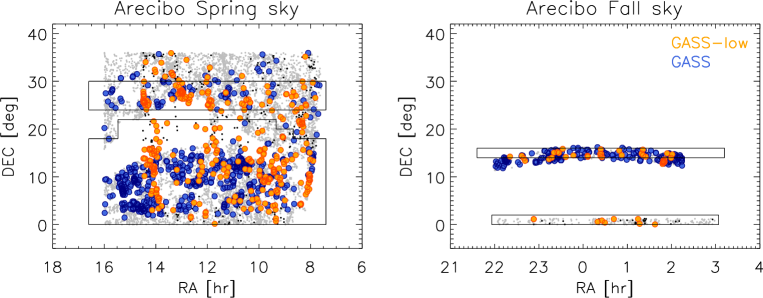
Figure 1: Sky distribution of galaxies in the GASS (blue) and GASS-low (orange) representative samples. Black and gray dots show the parent samples of the two surveys (GASS-low and GASS, respectively). The areas enclosed by thin black lines indicate the ALFALFA 70% footprint in the regions of interest.

The catalogs presented in our three GASS data releases (Catinella et al., 2010, 2012b, 2013) and in this work, as well as the full xGASS representative sample (see Section 2.2), are available on the xGASS website, along with all the Arecibo Hi spectra in digital format.

2.2 The xGASS representative sample

In order to increase survey efficiency we did not reobserve galaxies with good quality Hi detections in ALFALFA (based on the most recent data release available at the time of our observations, which was AA40 for GASS-low) or the Cornell Hi digital archive (Springob et al., 2005, hereafter S05). For ALFALFA, this refers to galaxies with detection code “1” (i.e., signal-to-noise SNR $\geq 6.5$); sources identified by code “2” (with lower SNR but coincident with an optical counterpart at the same redshift) were reobserved. Hence both GASS and GASS-low observed samples lack Hi-rich objects, which must be added back in the correct proportions to obtain data sets that are representative in terms of Hi properties. Because the two surveys cover different volumes and stellar mass regimes, we generate the two representative samples separately, taking advantage in both cases of the more recent 70% data release of ALFALFA (AA70). This is done slightly differently to the three GASS data releases. We explain below the procedure used to generate the xGASS representative sample, which is simply obtained by joining the GASS-low and (revised) GASS ones.

First, we divide each sample into two parts: inside and outside the AA70 footprint (see Fig. 1), which is given by the sky distribution of the 23,881 Hi-detected galaxies included in the publicly available catalog. The fraction of GASS-low and GASS parent samples included by this footprint are 74% and 75%, respectively. We compute the ALFALFA detection fraction in each stellar mass bin, $f_{\rm AA}$, defined as the ratio of number of galaxies $N_{\rm AA}$ detected by ALFALFA (code “1” only) and total number of sources $N_{\rm PS}$ in the parent sample, both restricted to the sky region with complete ALFALFA coverage and to the given stellar mass bin. Detection fractions decrease from 56.5% to 50.4% for GASS-low and from 16.2% to 13.9% for GASS going from the lowest to the highest stellar mass bin.

Second, we generate the representative sample for the subset within the AA70 footprint by adding the correct proportion of gas-rich, ALFALFA detections in each stellar mass bin. If $N_{\rm poor}$ is the number of observed galaxies in the given stellar mass bin that are not detected by ALFALFA, we obtain the number of gas-rich galaxies to be added as follows:

$$N_{\rm rich}=N_{\rm poor}\times\frac{N_{\rm AA}/N_{\rm PS}}{1-N_{\rm AA}/N_{\rm PS}}=N_{\rm poor}\times\frac{f_{\rm AA}}{1-f_{\rm AA}}$$ (1)

where $N_{\rm PS}$ is the number of galaxies in the parent sample within the AA70 footprint in the given stellar mass bin. We denote as $N_{\rm xGASS,rich}$ those galaxies that we observed but are also ALFALFA detections (for instance, GASS galaxies outside the AA40 footprint that turned out to be detected in AA70). These galaxies are not included in $N_{\rm poor}$, but we pick them first as gas-rich systems to be added to the sample. Next, we select $N_{\rm rich}-N_{\rm xGASS,rich}$ uniformly distributed, random galaxies from ALFALFA (giving first preference to sources with xCOLD GASS data) and we add them to $N_{\rm poor}+N_{\rm xGASS,rich}$ to obtain our representative sample.

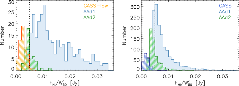
Figure 2: Histograms of the mean flux density across the detected Hi signal for GASS-low (left) and GASS (right) surveys, with ALFALFA detections (quality codes 1 and 2) in the corresponding volumes. Dotted lines indicate the value adopted to separate gas-rich from gas-poor galaxies in regions of sky not covered by ALFALFA (see text).

Third, we deal with the part of the sample outside the AA70 footprint. Here we need to estimate which galaxies would be detected by ALFALFA if the survey was complete. Because the sensitivity (or completeness) of ALFALFA depends on both flux and velocity width of the Hi signal (see Section 6 of Haynes et al., 2011), we inspect the histogram of the Hi integrated flux, $F_{\rm HI}$, divided by the observed velocity width, $W_{50}^{c}$ (measured at the 50% peak level and corrected for instrumental broadening and redshift only, see Appendix A) to decide where to set the threshold. Fig. 2 shows the $F_{\rm HI}/W_{50}^{c}$ histograms for GASS-low (left) and GASS (right) galaxies, compared with ALFALFA detections within the corresponding parent samples (code “1” and “2” are indicated in light blue and green, respectively). For both surveys we adopt a value of 0.005 Jy as our threshold (dotted lines), below which ALFALFA code “2” sources start dominating over high signal-to-noise ones. We verified that changing this number slightly does not have a significant effect on the final sample (changing the sky footprint over which detection fractions are computed, e.g. from AA40 to AA70, has a much larger effect). Then we use equation 1 to generate our representative samples, where $N_{\rm poor}$ now includes xGASS galaxies with $F_{\rm HI}/W_{50}^{c}<0.005$ Jy (i.e., below the ALFALFA detection limit) and $N_{\rm xGASS,rich}$ those above this threshold. The Hi-rich galaxies are extracted randomly from ALFALFA detections not already in the sample, trying to maximize the overlap with xCOLD GASS.

In our GASS papers, we treated the S05 Hi archive in a similar way as ALFALFA: we computed the fraction of parent sample galaxies with Hi data in the archive, $f_{\rm S05}$ (not including ALFALFA detections), and used equation 1 (with $f_{\rm S05}$ replacing $f_{\rm AA}$) to obtain the number of Hi-rich S05 galaxies to be added to the observed sample. While this does not affect our scaling relations (only 1.3% of the galaxies in the GASS DR3 representative sample were from S05 ), this is not entirely correct, because the S05 archive is not an Hi-blind survey, and thus $f_{\rm S05}$ is not a meaningful detection fraction. Thus we no longer add Hi-rich S05 galaxies to the observed sample.

We also considered including S05 galaxies below the ALFALFA detection threshold, together with the right complement of ALFALFA detections, to increase our statistics. This cannot be done in the GASS volume, where we would add 104 “Hi-poor” S05 galaxies, because the Hi archive sample is deeper than ALFALFA but still Hi-rich compared to GASS (thus we would bias our sample). However, this is not the case for the GASS-low volume, where there are only 13 “Hi-poor” S05 galaxies, all with gas fractions comparable to our observations. Thus we include these in our sample as if they had been observed by us (i.e. increasing $N_{\rm poor}$ in equation 1), and verified that our scaling relations are not affected by this choice.

The new GASS and GASS-low representative samples include 781 and 398 galaxies respectively, for a total 1179 xGASS galaxies. Fig. 3 summarizes the main properties of the sample. On the top row, the distributions of stellar mass, optical redshift from SDSS and Hi mass are shown separately for GASS (blue) and GASS-low (orange); non-detections are indicated in dark blue and brown, respectively. On the bottom row, we show the histograms of velocity width and gas fraction for the Hi detections, as well as the Hi detection fraction as a function of stellar mass for the two surveys. The $\sim$10% detection rate difference in the two overlapping stellar mass bins is most likely just noise (a couple more detections in GASS-low would have brought the detection rates into agreement). The observed velocity widths peak at $\sim$200 km s^-1 and 300 km s^-1 for GASS-low and GASS, respectively, so these are the values that we adopt to compute upper limits for the Hi mass of non-detections in the two surveys.

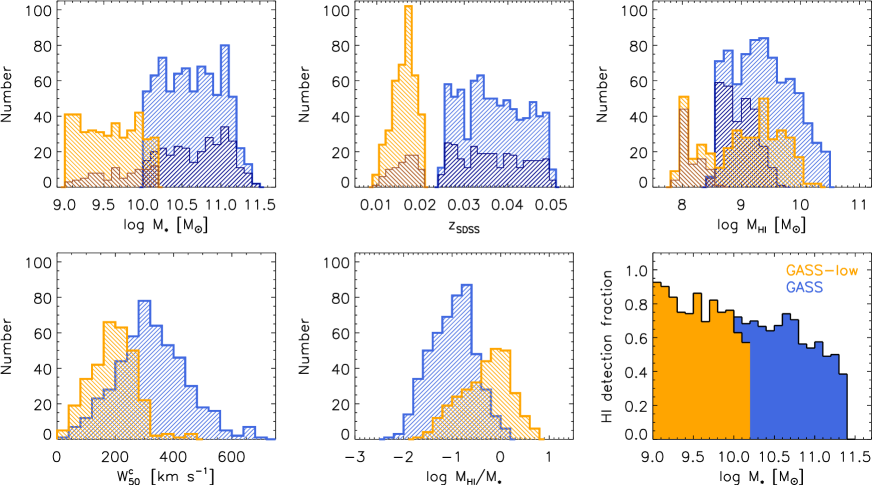
Figure 3: xGASS representative sample properties. Top row: Distributions of stellar mass, optical redshift and Hi mass for GASS (blue) and GASS-low (orange); dark blue and brown histograms indicate Hi non-detections for the two surveys, respectively. Bottom row: Distributions of Hi velocity width (corrected for instrumental broadening and redshift) and Hi gas fraction for detected galaxies; the Hi detection fraction (i.e., the ratio of detections to total) as a function of stellar mass is shown on the right panel (blue: GASS; orange: GASS-low).

2.2.1 Recovering a volume-limited sample

In our previous GASS work, we computed average scaling relations by weighting each measured gas fraction (detection or upper limit) by a factor $w_{i}(\rm M_{\star})$, in order to compensate for the flat stellar mass distribution imposed on the survey. Weights were computed using the parent sample as a reference, by binning both parent and representative samples by stellar mass and taking the ratio between the two histograms.

The xGASS representative sample has a similar problem, largely due to the difference in sample size between GASS and its low mass extension – low mass galaxies are under-represented and high mass ones over-represented, compared to what is expected for a volume-limited sample. This is illustrated in Figure 4, which shows the stellar mass distributions for GASS-low (orange histogram) and GASS (blue) representative samples, and for a volume-limited sample with the same total number of galaxies (black). The latter was obtained by sampling the local stellar mass function, parameterized as a double Schechter function by Baldry et al. (2012):

$$\Phi(\log M)d\log M=\ln(10)~{}e^{-x}\left[\phi_{1}^{*}~{}x^{(1+\alpha_{1})}+\phi_{2}^{*}~{}x^{(1+\alpha_{2})}\right]d\log M$$

where $x=10^{\log M-\log M^{*}}$, $\log M^{*}=10.66$ M_⊙, $\phi_{1}^{*}=0.00396$, $\phi_{2}^{*}=0.00079$, $\alpha_{1}=-0.35$ and $\alpha_{2}=-1.47$.

Thus, in this work we use the above stellar mass function to weight the gas fraction measurements when we compute average and median gas scaling relations; weights are simply obtained as the ratio between the black and the colored histograms in Figure 4 for the corresponding stellar mass bin and survey (GASS or GASS-low).

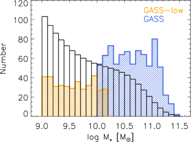
Figure 4: Stellar mass distributions for the xGASS representative sample (orange and blue indicate GASS-low and GASS subsets, respectively) and for a volume-limited sample with the same number of galaxies (see text).

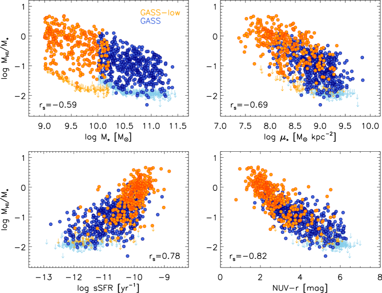
Figure 5: xGASS scaling relations: the Hi mass fraction is plotted as a function of stellar mass, stellar mass surface density, specific SFR and observed NUV$-r$ color. Circles and downward arrows indicate individual Hi detections and 5$\sigma$ upper limits, respectively, with the new GASS-low observations shown in orange. The Spearman’s correlation coefficient, $r_{s}$, is given on the bottom of each panel.

3 xCOLD GASS: The molecular gas survey

The COLD GASS survey measured homogeneous molecular gas masses, via the CO(1-0) emission line fluxes, for 366 galaxies extracted from the GASS sample (Saintonge et al., 2011). Because the IRAM beam size at the frequency of the observed CO(1-0) transition is 22″, aperture corrections were applied to extrapolate the measured CO line fluxes to total fluxes, as described in Saintonge et al. (2012). The extension of COLD GASS to a stellar mass of $10^{9}$ M_⊙, COLD GASS-low, includes IRAM observations of 166 additional galaxies, randomly extracted from the GASS-low parent sample (see Section 2.1.1). The two surveys taken together constitute xCOLD GASS, which includes 532 galaxies (333 detections) and is described in detail in Saintonge et al. (2017).

The CO(1-0) fluxes are converted into H₂ molecular masses using a multivariate conversion function, $\alpha_{CO}$, following Accurso et al. (2017). This function depends primarily on metallicity and secondarily on the offset from the star-forming main sequence, i.e. a parameter related to the strength of the UV radiation field; $\alpha_{CO}$ values for xCOLD GASS detections vary between 1 and 24.5 M_⊙ (K km s^-1 pc²)^-1, with an average of 4.44 (for comparison, the Galactic value is 4.35), taking into account the contribution of Helium. In this work, we use molecular gas masses without Helium contribution, $M_{\rm H2}$, to compute molecular-to-atomic hydrogen gas mass ratios.

The overlap between xCOLD GASS and the xGASS representative sample, which we refer to as xGASS-CO, includes 477 galaxies (290 CO detections) and is used in this work to investigate total gas scaling relations and H₂/Hi mass ratios. The remaining 55 galaxies with CO data are not included in xGASS because of one of the following reasons: (a) lack of Hi observations (13); (b) specifically targeted by COLD GASS for their very high specific SFRs, hence not preferentially selected for our representative sample (35, 2 of which were randomly picked as ALFALFA “code 1” sources); (c) S05 detections in GASS (7); or (d) ALFALFA “code 1” sources that were not selected because the stellar mass bin already included enough Hi-rich systems (2).

We recomputed the weights for xGASS-CO in order to recover the stellar mass distribution of a volume-limited sample, following the procedure described in Section 2.2.1. This sample is representative in terms of Hi content (we verified that the average Hi scaling relations obtained for xGASS and for xGASS-CO are consistent within the errors).

4 Results

We briefly revisit the main Hi gas fraction scaling relations, which extend our previous work (Catinella et al., 2010, 2012b, 2013) to lower stellar masses, and take advantage of the combined Hi and H₂ data set to investigate total gas scaling relations. Molecular gas scaling relations are presented in a companion paper (Saintonge et al., 2017). As discussed below, the distinct behavior of the atomic and molecular phases at low stellar masses motivates a more detailed discussion of the molecular-to-atomic gas mass ratio of galaxies along and outside the star-forming sequence.

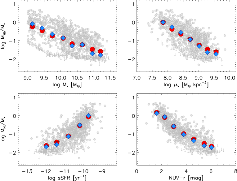
Figure 6: Average trends of Hi mass fraction as a function of stellar mass, stellar mass surface density, specific SFR and observed NUV$-r$ color for the xGASS sample. In each panel, large red circles and blue diamonds indicate weighted averages and weighted medians of the logarithms of the gas fractions, respectively (see text). Only bins including at least 20 galaxies are shown. Error bars are errors on the weighted means. These results are listed in Table 1. Small circles and downward arrows show individual Hi detections and non-detections (plotted at their upper limits), respectively.

4.1 Atomic gas fraction scaling relations

The Hi gas fraction scaling relations are presented in Figure 5. Clockwise from the top left, we show how the gas mass fraction $M_{\rm HI}$/$M_{\star}$ varies with stellar mass, stellar mass surface density, observed NUV$-r$ color and specific SFR (sSFR) for the full xGASS representative sample. Circles and downward arrows indicate Hi detections and Hi upper limits, respectively, with the new GASS-low survey shown in orange. The low mass galaxies smoothly extend GASS trends by one dex in stellar mass, probing higher gas fractions and sSFRs, bluer colors and lower stellar surface densities typical of disk-dominated systems. Because some of these relations do not appear linear (especially those with color and sSFR), we quantified their strength with the Spearman’s rank correlation coefficient, $r_{s}$, computed including the upper limits. The most significant correlation is with NUV$-r$ color ($r_{s}=-0.82$), with the $M_{\star}$ and $\mu_{\star}$ relations having significantly lower correlation coefficients ($r_{s}=-0.59$ and $-0.69$, respectively).

This is better seen in Figure 6, which quantifies the observed trends in terms of average (large red circles) and median (blue diamonds) gas fractions. The values plotted are weighted means and weighted medians of the logarithm of the gas fractions, where the weighting is applied to correct for the stellar mass bias of the sample (see Section 2.2.1); non-detections were set to their upper limits. For reference, small gray circles and downward arrows reproduce individual Hi detections and upper limits from Figure 5. Average and median gas fractions track each other closely in all plots, despite the fact that the underlying distributions are clearly not log-normal; however medians are preferable descriptors because less sensitive to the treatment of non-detections, which could lie anywhere below the upper limits. The values of the weighted average and median gas fractions shown in this figure are listed in Table 1. In order to quantify the scatter in these relations, we computed the difference between the 75th and 25th percentiles of the $\log$($M_{\rm HI}$/$M_{\star}$) distributions in each bin ($\Delta_{75-25,i}$, including the Hi non-detections at their upper limits), and took their arithmetic mean ($\bar{\Delta}$). We obtained $\bar{\Delta}=0.96,0.73,0.51$ and 0.43 dex for the $M_{\star}$, $\mu_{\star}$, sSFR and NUV$-r$ relations, respectively, with no clear trends in $\Delta_{75-25,i}$ with any of the above quantities (except for an artificially lower scatter in the two bins dominated by non-detections in each relation).

Figures 5 and 6 show that Hi gas fraction is more tightly related to NUV$-r$ color and sSFR, and both relations steepen in the star-forming sequence (approximately corresponding to NUV$-r$$<3$ mag and $\rm\log sSFR~{}[yr^{-1}]>-10.5$). This change of slope could be due to a saturation effect at the opposite end, where we hit the survey sensitivity limit and upper limits dominate the statistics. Contrary to the molecular gas fraction, which correlates more strongly with sSFR (Saintonge et al., 2017), the atomic gas fraction is more tightly related to NUV$-r$ color ($\bar{\Delta}=0.43$ dex), which traces dust-unobscured star formation (Bigiel et al., 2010).

Table 1: Hi gas fraction scaling relations for xGASS

$x$	$\langle x\rangle$	$\langle M_{\rm HI}/M_{\star}\rangle^{a}$	$(M_{\rm HI}/M_{\star})^{b}$	$N^{c}$
log $M_{\star}$	9.14	$-$0.242$\pm$0.053	$-$0.092	113
	9.44	$-$0.459$\pm$0.067	$-$0.320	92
	9.74	$-$0.748$\pm$0.069	$-$0.656	96
	10.07	$-$0.869$\pm$0.042	$-$0.854	214
	10.34	$-$1.175$\pm$0.037	$-$1.278	191
	10.65	$-$1.231$\pm$0.036	$-$1.223	189
	10.95	$-$1.475$\pm$0.033	$-$1.707	196
	11.20	$-$1.589$\pm$0.044	$-$1.785	86
log $\mu_{\star}$	7.85	$-$0.006$\pm$0.047	$-$0.002	61
	8.14	$-$0.377$\pm$0.050	$-$0.262	129
	8.42	$-$0.646$\pm$0.049	$-$0.561	160
	8.72	$-$0.926$\pm$0.044	$-$0.934	221
	9.01	$-$1.255$\pm$0.032	$-$1.303	326
	9.28	$-$1.475$\pm$0.031	$-$1.636	233
	9.56	$-$1.617$\pm$0.071	$-$1.734	30
log sSFR	$-$11.97	$-$1.633$\pm$0.022	$-$1.694	204
	$-$11.42	$-$1.442$\pm$0.032	$-$1.571	214
	$-$10.79	$-$1.109$\pm$0.034	$-$1.130	233
	$-$10.19	$-$0.539$\pm$0.033	$-$0.512	342
	$-$9.72	$-$0.063$\pm$0.041	$-$0.002	153
NUV$-r$	1.62	0.174$\pm$0.050	$-$0.130	39
	2.25	$-$0.090$\pm$0.028	$-$0.065	190
	2.98	$-$0.593$\pm$0.030	$-$0.577	198
	3.79	$-$0.987$\pm$0.033	$-$1.023	180
	4.59	$-$1.281$\pm$0.040	$-$1.362	155
	5.44	$-$1.514$\pm$0.026	$-$1.631	245
	6.04	$-$1.672$\pm$0.020	$-$1.725	144

Notes. $-$– ^aWeighted average of logarithm of gas fraction; Hi mass of non-detections set to upper limit. ^bWeighted median of logarithm of gas fraction; Hi mass of non-detections set to upper limit. ^cNumber of galaxies in the bin.

Hi gas fractions keep increasing with decreasing stellar mass, with no sign of a plateau, down to $M_{\star}$$=10^{9}$ M_⊙ (median values of $M_{\rm HI}$/$M_{\star}$ increase from 2% to 81% from the highest to the lowest stellar mass bin). This is consistent with the relation for Hi-rich galaxies detected by ALFALFA, which shows a flattening only below $M_{\star}$$\sim$$10^{8.5}$ M_⊙ (Huang et al., 2012). The correlation between Hi gas fraction and stellar mass has the largest scatter ($\bar{\Delta}=0.96$ dex). This is not surprising, as we already showed in previous work that variations of atomic gas fraction at fixed stellar mass strongly correlate with star formation activity (Brown et al., 2015). By applying spectral stacking to a large stellar mass-selected sample with Hi data from ALFALFA, Brown et al. (2015, see their Fig. 5) demonstrated that this relation is the result of a more physical correlation between Hi content and SFR, combined with the bimodality of galaxies — dividing up their sample in three NUV$-r$ color bins, roughly corresponding to blue sequence, red sequence and green valley, they obtained three parallel relations with significantly flatter slope.

Interestingly, the relation with stellar surface density has lower scatter ($\bar{\Delta}=0.73$ dex), indicating that the correlation between gas fraction and stellar content improves when we take into account the size of the stellar disk (even if estimated as a 50% effective radius). As noted before, a distinct difference between the $M_{\star}$ and $\mu_{\star}$ relations is the distribution of the non-detections, which are spread across the stellar mass range but pile up in the bulge-dominated region ($\log$ $\mu_{\star}$[M_⊙ kpc^-2] $\gtrsim 8.5$) – above this threshold, both Hi and H₂ detection rates drop significantly (Catinella et al., 2010; Saintonge et al., 2011). Galaxies in the lowest stellar surface density bin have median gas fractions of 100%, i.e. have the same amount of mass in Hi gas and in stars; those with the bluest NUV$-r$ colors are gas-dominated, reaching median gas fractions of 135%.

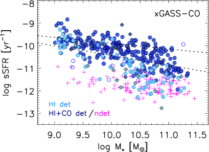
Figure 7: Specific SFR plotted as a function of stellar mass for the subset of xGASS with CO data. Filled circles indicate galaxies detected in both Hi and CO (dark blue) or Hi only (light blue); black-edged diamonds are Hi detections affected by beam confusion. Empty circles are CO detections with Hi upper limits, and magenta crosses are non-detections in both Hi and CO lines. Dotted lines show the star-forming sequence adopted in this work (see text), and correspond to the 1$\sigma$ deviation above and below the average.

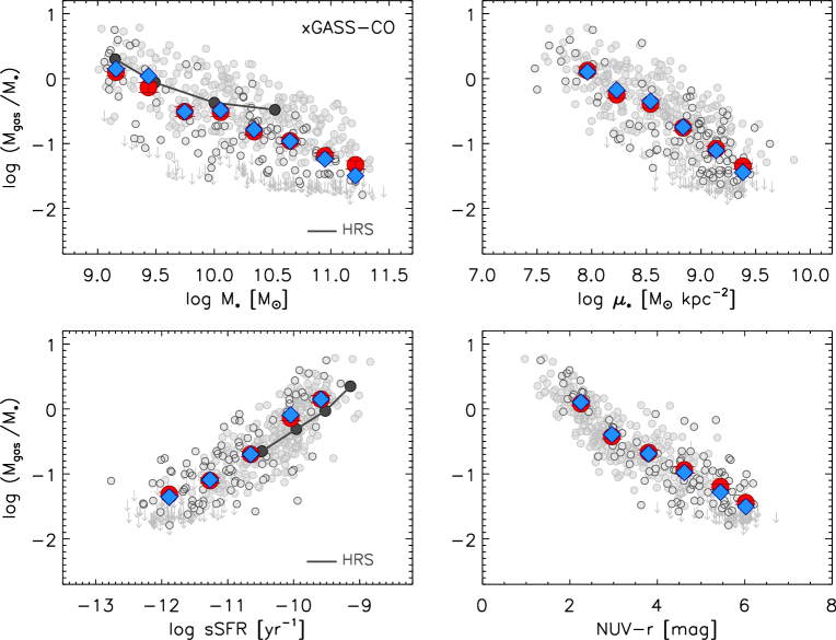
Figure 8: Total gas fraction scaling relations for the xGASS-CO sample. Small gray circles and downward arrows show individual detections and non-detections in both Hi and CO lines; gray circles with darker contours indicate galaxies detected in Hi or CO, but not both. As in Figure 6, large red circles and blue diamonds are weighted averages and weighted medians of the logarithms of the (total) gas fractions. These results are listed in Table 2. Black circles connected by lines in the left plots show the results from the Herschel Reference Survey (HRS; Boselli et al., 2014b).

4.2 Total gas fraction scaling relations

In the rest of this paper we restrict our analysis to the subset of xGASS with IRAM observations, xGASS-CO, which includes 477 galaxies (see Section 3).

Figure 7 shows the distribution of this sample in the specific SFR versus stellar mass plane, with points color-coded according to their detection status in the Hi and H₂ surveys. About 57% of the sample is detected in both lines (filled, dark blue circles), 16% is detected only in Hi (light blue) and 23% has no cold gas detection (crosses). As expected, galaxies on or above the star-forming main sequence (SFMS, dotted lines; see below) are typically Hi and H₂ detections, except at the low stellar mass end, where metallicities are lower and CO emission is more challenging to detect. We marked with black-edged diamonds 39 galaxies (8% of xGASS-CO) with Hi emission that is confused within the Arecibo beam (see Appendices); together with the non-detections in both gas phases, these objects are excluded from the analysis of molecular-to-atomic gas mass ratios in the next section. It is interesting to note that 17 galaxies (4% of our sample, empty circles) are detected in CO only; of these, 9 are satellites in groups with 19 or more members according to the Yang et al. (2007) group catalog and are all located in the bottom half of the SFMS or below it, suggesting that environmental effects in these large groups might have depleted the Hi reservoirs, but not as far inside as the optical disk, thus leaving the H₂ content mostly unaffected (Fumagalli et al., 2009; Boselli et al., 2014a; Cortese et al., 2016).

We defined our own SFMS using the full xGASS representative sample. Briefly, we binned the points in the sSFR- stellar mass plot (not shown) in stellar mass intervals of 0.25 dex, and fit Gaussians to the resulting sSFR distributions; this works well below $M_{\star}$$\sim$$10^{10}$ M_⊙, where the red sequence is almost absent. At higher stellar masses, we fit Gaussians with fixed centers based on the extrapolation of the relation at lower $M_{\star}$, and use only sSFRs above the relation to constrain the widths of the Gaussians. This procedure (illustrated in more detail in Janowiecki et al. in preparation) yields the following expression:

$$\log sSFR_{MS}=-0.344(\log M_{\star}-9)-9.822$$ (2)

with a standard deviation given by:

$$\sigma_{MS}=0.088(\log M_{\star}-9)+0.188$$

The limits corresponding to $\pm 1\sigma_{MS}$ from the SFMS are shown as dotted lines in Figure 7.

Figure 8 shows the scaling relations for the total gas (where $M_{\rm gas}=1.3(M_{\rm HI}+M_{\rm H2})$, including the Helium contribution). As in Figure 6, weighted average (large red circles) and median (blue diamonds) gas fractions are plotted on top of individual measurements (small gray symbols; circles with darker contours are galaxies detected in either Hi or CO), with the same axis scales for comparison. Median total gas fractions (computed including all detections and upper limits) decrease from 141% to 3% over our stellar mass range; the galaxies with the highest total gas fractions in our sample have six times more mass in cold gas than stars.

The observed trends are qualitatively similar to the ones seen for the atomic phase, but with slightly smaller scatter, especially in the relations between gas fraction and stellar mass or stellar surface density. If we quantify the dispersions of these relations with the parameter $\bar{\Delta}$ defined in the previous section, i.e. the average difference between the 75th and 25th percentiles of the $\log$($M_{\rm gas}$/$M_{\star}$) distributions in each bin, we obtain $\bar{\Delta}=0.70,0.61,0.47$ and 0.36 dex for the $M_{\star}$, $\mu_{\star}$, sSFR and NUV$-r$ relations. These should be compared with the dispersions of the Hi scaling relations computed for the same xGASS-CO sample, which are $\bar{\Delta}=0.81,0.69,0.50$ and 0.40 dex, respectively. This difference is most likely due to the fact that the total gas fractions have smaller dynamic range than the atomic ones.

Overall, the similarity between atomic and total gas scaling relations is not surprising, as galaxies in this stellar mass regime in the local Universe typically have cold gas reservoirs that are Hi-dominated (Saintonge et al., 2011; Boselli et al., 2014b; Saintonge et al., 2016, see also next section).

Our total gas scaling relations confirm and extend to higher stellar mass the results of Boselli et al. (2014b), obtained for field late-type galaxies detected in both Hi and CO lines in the Herschel Reference Survey (HRS; Boselli et al., 2010), assuming a luminosity-dependent $\rm X_{CO}$ conversion factor to compute molecular gas masses. For reference, the HRS results are shown as black circles connected by lines in Fig. 8 (left panels). The agreement with their stellar mass relation in the overlap interval ($\log$$M_{\star}$ [M_⊙] $<10.5$) is excellent, except for their highest stellar mass bin, which has a total gas fraction 0.4 dex higher than ours, probably due to limited statistics of the HRS at the high $M_{\star}$ end. The relation with sSFR for the HRS galaxies has the same slope but is slightly offset towards lower gas fractions (by $\sim$0.2 dex); however the two samples overlap by only $\sim$1.5 dex in sSFR.

Interestingly, Boselli et al. (2014b) noted that the HRS relationships involving molecular gas fractions are always flatter than those with total gas fraction. This is confirmed by our sample (Accurso et al., 2017; Saintonge et al., 2017). Indeed, thanks to the larger dynamic range in $M_{\star}$ and $\mu_{\star}$ of xCOLD GASS, we detect a clear break in the molecular gas relations, which suddenly flatten below $\log$ $M_{\star}$[M_⊙] $=10.5$ and $\log$ $\mu_{\star}$[M_⊙ kpc^-2] $=8.5$ (see Accurso et al., 2017; Saintonge et al., 2017). As seen in Figure 8, there is no trace left of such flattening in the total gas relations. The difference between atomic and molecular gas fraction relations below these stellar mass and stellar surface density limits is striking, and warrants a closer look at the molecular-to-atomic mass ratio in the next section.

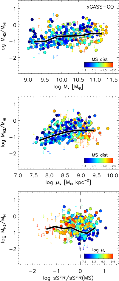
Figure 9: Molecular-to-atomic gas mass ratio as a function of stellar mass (top), stellar surface density (middle) and deviation from the star-forming main sequence (bottom). In each panel, circles are galaxies with both Hi and CO detections, downward arrows are Hi detections with CO upper limits, and upward arrows are CO detections with Hi upper limits. Galaxies are color-coded by distance from the SF sequence in the top two panels, and by $\mu_{\star}$ in the bottom one. Thick lines show running medians; only medians computed with at least 10 galaxies are shown.

4.3 Molecular-to-atomic gas mass ratios

In our previous work we investigated the relation between Hi and H₂ content for the initial release of the GASS+COLD GASS sample, and found that the molecular-to-atomic gas mass ratio, $R_{\rm mol}\equiv M_{\rm H2}/M_{\rm HI}$, weakly increases with stellar mass, stellar surface density and NUV$-r$ color, but with over 0.4 dex of scatter (Saintonge et al., 2011). We also showed how $R_{\rm mol}$ varies across the SFR-$M_{\star}$ plane for the full GASS+COLD GASS sample, and identified a region of unusually high values of $R_{\rm mol}$ ($>0.7$) at high stellar masses and SFRs ($\log M_{\star}[M_{\odot}]>10.8$ and $\rm-10.4<\log~{}sSFR[yr^{-1}]<-9.6$; Saintonge et al. 2016). These galaxies are characterized by young stellar populations in their central regions (based on their $\rm D_{n}4000$ from SDSS fiber spectroscopy) and important bulge components ($\log\mu_{\star}\sim 8.9$). Here we extend these studies to lower stellar mass, focusing on the relation between galaxies within or outside the SFMS defined in the previous section. Galaxies with non-detections in both Hi and H₂ (magenta crosses in Fig. 7) are excluded from this analysis, because their $R_{\rm mol}$ is unconstrained; we also exclude Hi-confused detections (black-edged diamonds in Fig. 7), which leaves us with a sample of 328 galaxies.

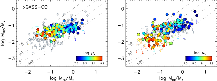
Figure 10: Comparison between H₂ and Hi gas fractions. Circles are galaxies detected in both Hi and H₂; downward and leftward arrows are H₂ and Hi upper limits, respectively. The two panels highlight galaxies within 1$\sigma$ from the SFMS (left; see Fig. 7) and outside the SFMS (right panel), color-coded according to their stellar surface density as indicated. Gray symbols in each panel show the excluded galaxies (i.e., correspond to the colored points in the other panel). Also shown are lines of constant molecular-to-atomic gas mass ratio, with $M_{\rm H2}$/$M_{\rm HI}$ values as labeled.

Figure 9 (top two panels) shows the molecular-to-atomic gas mass ratio as a function of stellar mass and stellar surface density for our sample; thick lines indicate running weighted medians of the logarithm of $R_{\rm mol}$. The median $R_{\rm mol}$ slowly increases with both stellar mass (from 9% to 28%) and stellar surface density (from 6% to 25%; see Table 3). A similar trend with stellar mass was also found by the APEX Low-redshift Legacy Survey for MOlecular Gas (ALLSMOG, Bothwell et al., 2014) and the HRS (Boselli et al., 2014b), which both combined COLD GASS data with new observations probing stellar masses below $10^{10}M_{\odot}$. Furthermore, galaxies in the top two panels of Figure 9 are color-coded according to their distance from the SFMS (i.e., $\rm dist_{MS}=\log sSFR-\log sSFR_{MS}$, see equation 2); negative values (redder colors) correspond to systems below the SFMS. Galaxies located below the SFMS typically have high stellar surface densities; this is better seen in the bottom panel, where $R_{\rm mol}$ is plotted as a function of distance from the SFMS, and color-coded by $\mu_{\star}$. On and above the SFMS (dashed line), bulge-dominated systems are displaced towards higher $R_{\rm mol}$ values.

The scatter in these plots is quite large, with $M_{\rm H2}$/$M_{\rm HI}$ ratios that vary by almost two orders of magnitude across our sample. As seen in the middle panel, galaxies below the SFMS (which are typically bulge-dominated) seem to follow a different relation from star-forming disks. This qualitatively agrees with the observation that HRS early-type galaxies detected in Hi do not follow the same gas scaling relations as late-type ones (Boselli et al., 2014b). However, it is unclear if the observed scatter correlates more strongly with deviation from the SFMS or stellar surface density.

In order to gain further insight into what regulates the molecular-to-atomic gas mass ratio of our sample, we compare Hi and H₂ gas fractions directly in Figure 10. In the left panel, galaxies on the SFMS are color-coded by stellar surface density; the right panel shows the complementary set of galaxies located outside the SFMS, with the same color coding. Looking at the right panel first, there is a general trend of increasing molecular gas fractions for increasing $M_{\rm HI}$/$M_{\star}$, with a clear dependence on stellar surface density. As can be seen, more bulge-dominated systems (redder colors in the figure) have systematically lower atomic and molecular gas fractions, while spanning the full range of $R_{\rm mol}$. Very interestingly, and contrary to the rest of the sample, the relation for SFMS galaxies (left) is nearly flat – selecting galaxies within 1$\sigma$ of the SFMS restricts $M_{\rm H2}$/$M_{\star}$ to vary within a dex, whereas atomic gas fractions still span almost the entire range of the full sample. This is highlighted by the lines of constant molecular-to-atomic gas mass ratio, which increases from 3% to 100% from bottom to top, and shows that the observed variation of $R_{\rm mol}$ is mostly driven by changes of the atomic gas reservoir – not the molecular one.

This finding suggests that the scatter in the total gas scaling relations might also be related to the variation of molecular-to-atomic gas mass ratio, which is indeed the case. This is demonstrated in Figure 11, which presents the relations of Figure 8 with points color-coded by $R_{\rm mol}$; gray arrows are galaxies with upper limits in both Hi and H₂  for which $R_{\rm mol}$ is not defined. The variation of total gas fraction is clearly driven by a change in molecular-to-atomic gas mass ratio in all these plots. The secondary dependence on $R_{\rm mol}$ is most prominent at fixed specific SFR, where galaxies with smaller total gas reservoirs have larger values of $R_{\rm mol}$.

Lastly, the left panel of Figure 9 shows that, because H₂ gas fractions are to first order roughly constant on the SFMS, the decrease of Hi gas fractions leads to higher $R_{\rm mol}$ for bulge-dominated systems, as observed in Figure 9. It is tempting to interpret these trends with stellar stellar surface density as suggestive of a causal link between galaxy structure and gas content. However, we obtain very similar results if we color-code the galaxies in this figure by stellar mass (not shown), pointing out the difficulty of separating the effects of mass and structure using global measurements.

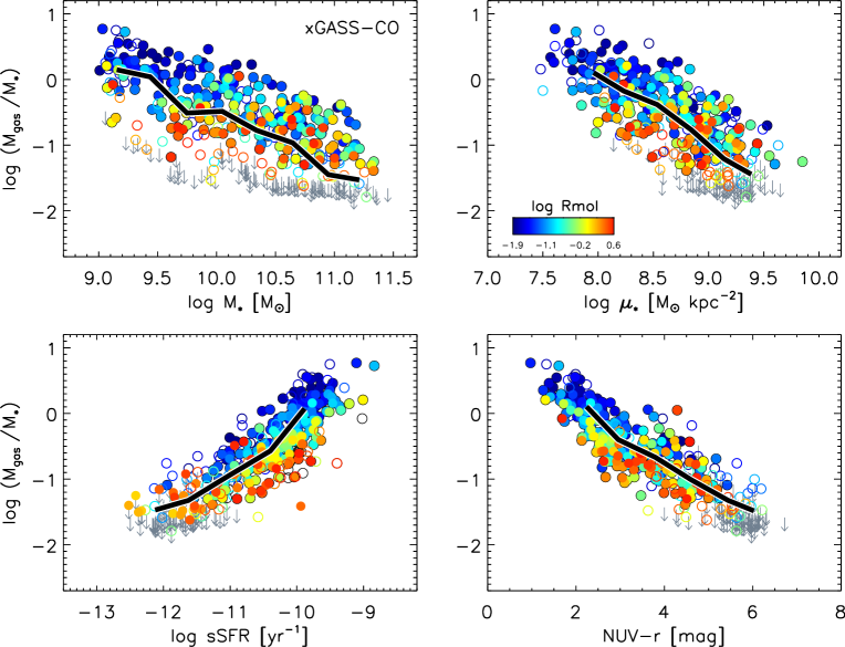
Figure 11: Total gas fraction scaling relations, color-coded by molecular-to-atomic gas mass ratio. Empty circles indicate galaxies not detected in either Hi or H₂, and gray downward arrows are systems with upper limits in both gas phases, for which $R_{\rm mol}$ is not defined. This sample does not include Hi-confused galaxies, hence running medians (thick lines) are not identical to those in Figure 8 (blue diamonds).

Table 2: Total gas fraction scaling relations for xGASS-CO

$x$	$\langle x\rangle$	$\langle M_{\rm gas}/M_{\star}\rangle^{a}$	$(M_{\rm gas}/M_{\star})^{b}$	$N^{c}$
log $M_{\star}$	9.16	$-$0.098$\pm$0.064	$-$0.148	41
	9.44	$-$0.136$\pm$0.077	$-$0.040	43
	9.75	$-$0.509$\pm$0.076	$-$0.511	54
	10.05	$-$0.518$\pm$0.062	$-$0.485	69
	10.34	$-$0.817$\pm$0.055	$-$0.785	75
	10.65	$-$0.958$\pm$0.048	$-$0.965	89
	10.95	$-$1.190$\pm$0.048	$-$1.238	74
	11.21	$-$1.328$\pm$0.064	$-$1.496	31
log $\mu_{\star}$	7.96	$-$0.125$\pm$0.057	$-$0.104	44
	8.23	$-$0.247$\pm$0.056	$-$0.176	65
	8.54	$-$0.390$\pm$0.067	$-$0.348	64
	8.84	$-$0.757$\pm$0.049	$-$0.746	110
	9.14	$-$1.079$\pm$0.040	$-$1.106	130
	9.38	$-$1.348$\pm$0.045	$-$1.443	46
log sSFR	$-$11.89	$-$1.313$\pm$0.032	$-$1.356	87
	$-$11.27	$-$1.102$\pm$0.042	$-$1.089	91
	$-$10.65	$-$0.698$\pm$0.042	$-$0.699	88
	$-$10.05	$-$0.141$\pm$0.039	$-$0.092	149
	$-$9.59	$-$0.151$\pm$0.056	$-$0.150	44
NUV$-r$	2.25	0.082$\pm$0.034	$-$0.104	95
	2.96	$-$0.424$\pm$0.035	$-$0.394	80
	3.80	$-$0.670$\pm$0.042	$-$0.689	69
	4.62	$-$0.938$\pm$0.052	$-$0.978	76
	5.44	$-$1.197$\pm$0.042	$-$1.282	82
	6.02	$-$1.442$\pm$0.026	$-$1.504	52

Notes. $-$– ^aWeighted average of logarithm of gas fraction; Hi mass of non-detections set to upper limit. ^bWeighted median of logarithm of gas fraction; Hi mass of non-detections set to upper limit. ^cNumber of galaxies in the bin.

Table 3: Molecular-to-atomic gas mass ratio scaling relations for xGASS-CO

$x$	$\langle x\rangle$	$\langle$$M_{\rm H2}$/$M_{\rm HI}$$\rangle^{a}$	($M_{\rm H2}$/$M_{\rm HI}$)b	$N^{c}$
log $M_{\star}$	9.18	$-$0.903$\pm$0.070	$-$1.044	44
	9.53	$-$0.865$\pm$0.079	$-$1.003	38
	9.88	$-$0.660$\pm$0.073	$-$0.704	53
	10.22	$-$0.704$\pm$0.059	$-$0.691	59
	10.59	$-$0.662$\pm$0.057	$-$0.659	65
	10.91	$-$0.530$\pm$0.058	$-$0.521	50
	11.20	$-$0.578$\pm$0.075	$-$0.559	18
log $\mu_{\star}$	7.67	$-$1.132$\pm$0.066	$-$1.228	14
	7.96	$-$1.018$\pm$0.069	$-$1.032	41
	8.23	$-$0.682$\pm$0.066	$-$0.870	57
	8.53	$-$0.683$\pm$0.072	$-$0.706	49
	8.84	$-$0.583$\pm$0.060	$-$0.606	79
	9.13	$-$0.603$\pm$0.054	$-$0.591	70
	9.40	$-$0.602$\pm$0.122	$-$0.603	14

Notes. $-$– ^aWeighted average of logarithm of $R_{\rm mol}$; Hi and H₂ masses of non-detections set to upper limits. ^bWeighted median of logarithm of $R_{\rm mol}$; Hi and H₂ masses of non-detections set to upper limits. ^cNumber of galaxies in the bin.

5 Comparison with models

Gas fraction scaling relations for representative samples have a unique constraining power for galaxy formation models (e.g., Lagos et al., 2014, 2015; Popping, Somerville & Trager, 2014; Popping, Behroozi & Peeples, 2015; Bahé et al., 2016; Davé et al., 2017). Modern cosmological semi-analytic and hydrodynamical simulations successfully reproduce overall stellar and star formation properties of galaxies over cosmic time, but must rely on sub-resolution prescriptions to partition the cold gas into atomic and molecular phases and form stars. Comparisons between observed gas scaling relations from stellar mass-selected samples and simulated ones have highlighted areas where models need improvement (e.g., Kauffmann et al., 2012; Brown et al., 2017; Stevens & Brown, 2017; Zoldan et al., 2017).

In our companion paper (Saintonge et al., 2017), we compared Hi and H₂ gas fractions as a function of stellar mass with predictions from two large, state-of-the-art hydrodynamical simulations, MUFASA (Davé, Thompson & Hopkins, 2016; Davé et al., 2017) and the Evolution and Assembly of GaLaxies and their Environments (EAGLE, Schaye et al. 2015. We used their high resolution Recal-L025N0752 run).

Briefly, MUFASA directly tracks the amount of molecular gas formed in galaxies using a sub-resolution prescription (broadly following Krumholz, McKee & Tumlinson 2009). The atomic fraction is obtained by subtracting the molecular fraction from the neutral (self-shielded against the cosmic metagalactic flux) gas, and the global Hi content of a galaxy is just the sum of the atomic gas that is bound to it.

For the EAGLE simulations, the partition of the ISM into its different phases was implemented by Lagos et al. (2015) in post-processing. The separation between ionized and neutral (self-shielded) gas is done according to the same prescription adopted by MUFASA (based on Rahmati et al. 2013); the neutral gas is then divided into Hi and H₂ phases following Gnedin & Kravtsov (2011, GK11) or Krumholz (2013, K13). Both recipes give H₂ fractions that depend on gas metallicity and strength of the interstellar radiation field, but the partition into Hi and H₂ phases relies on the assumption that the warm and cold components of the ISM are in pressure equilibrium (K13) or is based on metallicity, since H₂ formation happens on dust grains (GK11).

The comparison with our results showed that both MUFASA and EAGLE simulations reproduce reasonably well the Hi gas fractions in galaxies with $\log M_{\star}[M_{\odot}]<10.5$, but significantly underpredict the amount of cold atomic gas in more massive galaxies. Contrary to the Hi phase, predictions of H₂ gas fractions are very sensitive to the subgrid physics assumed to partition the ISM, and we found that none of these hydrodynamical simulations reproduce the molecular gas content of galaxies with $\log M_{\star}[M_{\odot}]<10.5$ particularly well (Saintonge et al., 2017). The best agreement is with the EAGLE K13 prescription, whereas EAGLE GK11 and MUFASA produce galaxies with too much molecular gas.

Interestingly, despite the fact that Hi and H₂ gas fractions are not individually well reproduced by these hydrodynamical simulations across the full stellar mass range of our sample, Figure 12 shows that the molecular-to-atomic gas mass ratio predicted by EAGLE is in overall better agreement with our observations (gray symbols, with the solid black line showing the median relation). In this figure, red and blue lines indicate median $R_{\rm mol}$ values from MUFASA and Recal-L025N0752 EAGLE run respectively; for the latter, light and dark blue lines correspond to the K13 and GK11 prescriptions. In order to be consistent with our observations, we applied our gas fraction limits to the simulated data sets, and excluded galaxies that would not be detected in both Hi and H₂ before computing the medians. MUFASA galaxies have molecular-to-atomic gas mass ratios $\sim$0.4 dex higher than observed. This is because, to partly compensate for its lower resolution, MUFASA effectively employs a lowered density threshold for forming H₂, which results in more ISM gas being molecular rather than atomic at a given stellar mass. The EAGLE K13 model provides an excellent match to our data, whereas the GK11 version slightly but systematically overestimates $R_{\rm mol}$. We note that, while Hi gas fractions above $\log M_{\star}[M_{\odot}]$$\sim$10.2, are similarly underestimated in both subgrid implementations, the H₂ fractions are underestimated by K13 (thus getting $R_{\rm mol}$ approximately correct) and overestimated for GK11, resulting in higher molecular-to-atomic gas mass ratios. This shows the importance of testing multiple gas scaling relations to constrain the physics implemented in simulations.

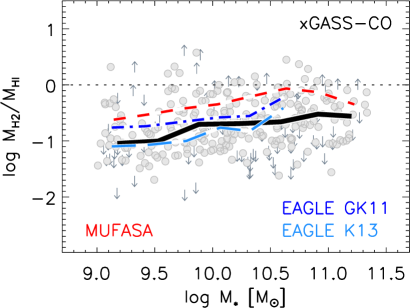
Figure 12: Comparison with hydrodynamical simulations. The molecular-to-atomic gas mass ratio as a function of stellar mass is reproduced from the top panel of Fig. 9 (gray points), along with the median relation for our sample (black line). Predictions from MUFASA (Davé, Thompson & Hopkins, 2016) and EAGLE (Lagos et al., 2015) hydrodynamical models are shown as red and blue lines, respectively. The two EAGLE models differ for the prescription adopted to partition the cold gas into atomic and molecular phases (GK11: Gnedin & Kravtsov 2011; K13: Krumholz 2013). The horizontal dotted line is at $M_{\rm H2}$/$M_{\rm HI}$ $=1$, separating atomic- from molecular-dominated systems.

6 Summary and conclusions

In this paper we presented xGASS, the culmination of several years of effort to gather deep Hi observations for a stellar mass-selected sample of $\sim$1200 galaxies with homogeneously measured optical and SF properties. xGASS is the combination of the original GASS survey, which started in 2008 and targeted galaxies with stellar masses larger than $10^{10}$ M_⊙, and its extension to $M_{\star}=10^{9}$ M_⊙. Together, these surveys required $\sim$1300 hours of Arecibo telescope time. Our unique approach of carrying out gas fraction-limited observations down to $M_{\rm HI}$/$M_{\star}$$\sim$2% allowed us to obtain stringent upper limits, which are essential to interpret variations of gas content as a function of galaxy properties.

We release here Hi catalogs and spectra for the complete low mass extension of GASS, which includes new Arecibo observations of 208 galaxies. By adding the correct proportion of ALFALFA Hi-rich systems (not targeted by us to increase survey efficiency) to GASS and GASS-low data sets, we obtained a representative sample (in terms of Hi content) of 1179 galaxies with stellar mass $10^{9}\leq M_{\star}/M_{\odot}\leq 10^{11.5}$ in the local Universe ($0.01\leq z\leq 0.05$).

In addition to extending the Hi scaling relations by one decade in stellar mass, we quantified total gas fraction scaling relations for the subset of 477 galaxies with molecular hydrogen mass estimates available, and explored molecular-to-atomic gas mass variations for galaxies detected in at least one of the two gas phases. H₂ masses were obtained as part of the xCOLD GASS follow-up survey, which measured the CO(1-0) line emission of xGASS galaxies using the IRAM 30m radio telescope (Saintonge et al., 2017). Our main results are summarized below.

• Atomic gas fractions increase from 2% (set by the limit of our observations) to 81% with decreasing stellar mass, with no sign of a plateau. The tightest relation is with NUV$-r$ color, which traces dust-unobscured star formation (as opposed to molecular gas fractions that correlate more strongly with sSFR, Saintonge et al. 2017).

• On average, galaxies have gas reservoirs that remain dominated by atomic hydrogen across the full range of stellar masses probed by our survey (see also Fig. 12). Molecular-to-atomic hydrogen mass ratios weakly increase with stellar mass from 9% to 27%, but varying by two orders of magnitude across the sample.

• Total gas fraction scaling relations closely resemble atomic ones, as expected from the fact that Hi is the dominant gas phase. Below $\log M_{\star}/M_{\odot}\sim 9.5$, the median galaxy has more mass in cold gas than stars. The scatter in the total gas fraction relations is driven by changes in $R_{\rm mol}$. At fixed specific SFR, galaxies with larger total gas reservoirs have smaller molecular-to-atomic gas mass ratios.

• For galaxies on the star-forming sequence, variations of $R_{\rm mol}$ are mostly driven by changes of the Hi reservoirs, with a clear dependence on stellar surface density. Bulge-dominated systems have $M_{\rm H2}$/$M_{\rm HI}$ ratios that are typically three times larger than those of disk-dominated galaxies. This highlights once again the importance of galaxy structure, as traced by stellar surface density, in relation to the cold gas content of galaxies (see also Catinella et al., 2010; Saintonge et al., 2011, 2012; Brown et al., 2015).

When interpreting these results, one has to bear in mind that Hi and H₂ line fluxes are measured with radio telescopes with vastly different beams ($\sim$3.5 arcmin for Arecibo and $\sim$22 arcsec for IRAM). We apply aperture corrections to recover global H₂ masses, but nonetheless it is well known that most of the Hi is distributed in the outer parts of galaxy disks, beyond the H₂-dominated regions. Thus our $M_{\rm H2}$/$M_{\rm HI}$ ratios carry information on the global Hi and H₂ gas reservoirs available for future star formation, more than on the detailed conversion between the two. Even with this caveat, it remains very intriguing to investigate the reason(s) for the systematic variation of the molecular-to-atomic gas mass ratio with stellar surface density, and ultimately presence of a bulge component. While it remains difficult to establish if stellar mass or structure is more important in connection with the gas content of galaxies (at least using global quantities), there is no doubt that part of the scatter in all the relations presented in this work must be due to the fact that we normalize gas masses by stellar mass, which includes the bulge component, whereas the gas is found in the disk. We will address this issue in future work, by performing accurate photometric bulge-to-disk decompositions for xGASS galaxies to separate the total stellar mass into bulge and disk contributions, $M_{\star,B}$ and $M_{\star,D}$. We will then be able to investigate gas fraction scaling relations for the disk component alone (i.e., plotting $M_{\rm HI}/M_{\star,D}$) and determine if and how these are affected by the presence of a bulge.

Statistical measurements of the cold gas content for stellar mass-selected samples are a crucial test-bed for models of galaxy formation. We presented an example by comparing molecular-to-atomic gas mass ratios measured from our sample with two state-of-the-art hydrodynamical simulations, MUFASA and EAGLE, and noted how sometimes good agreement is obtained overall, even though the underlying distributions are not well reproduced. This is a complex parameter space, with several systematic trends that are still not completely understood, thus it is essential to test simulations with the largest possible combination of ISM components and galaxy properties – something that our large, homogeneous and very sensitive xGASS and xCOLD GASS surveys were precisely designed to provide.

Appendix A: Data Release

We present here SDSS postage stamp images, Arecibo Hi-line spectra, and catalogs of optical, UV and Hi parameters for the 208 GASS-low galaxies. The content of the tables is described below; notes on individual objects (marked with an asterisk in the last column of Tables A2 and A3) are reported in Appendix B.

SDSS and GALEX data.
Table A1 lists optical and UV quantities for the 208 GASS-low galaxies, ordered by increasing right ascension:

Cols. 1 and 2: GASS and SDSS identifiers. Galaxies with six digit GASS IDs are part of GASS-low.

Col. 3: UGC (Nilson, 1973), NGC (Dreyer, 1888) or IC (Dreyer, 1895, 1908) designation, or other name, typically from the Catalog of Galaxies and Clusters of Galaxies (CGCG; Zwicky et al., 1961), or the Virgo Cluster Catalog (VCC; Binggeli, Sandage & Tammann, 1985).

Col. 4: SDSS redshift, $z_{\rm SDSS}$. The typical uncertainty of SDSS redshifts for this sample is 0.0002.

Col. 5: base-10 logarithm of the stellar mass, $M_{\star}$, in solar units. Stellar masses are obtained from the SDSS DR7 MPA/JHU catalog (see footnote 2 in section 2.3) and assume a Chabrier (2003) initial mass function. Over our stellar mass range, these values are believed to be accurate to better than 30%.

Col. 6: radius containing 50% of the Petrosian flux in z-band, $R_{50,z}$, in arcsec.

Cols. 7 and 8: radii containing 50% and 90% of the Petrosian flux in r-band, $R_{50}$ and $R_{90}$ respectively, in arcsec.

Col. 9: base-10 logarithm of the stellar mass surface density, $\mu_{\star}$, in M_⊙ kpc^-2. This quantity is defined as $\mu_{\star}=M_{\star}/(2\pi R_{50,z}^{2})$, with $R_{50,z}$ in kpc units (computed using angular distances).

Col. 10: Galactic extinction in r-band, ext_r, in magnitudes, from SDSS.

Col. 11: r-band model magnitude from SDSS, $r$, corrected for Galactic extinction.

Col. 12: minor-to-major axial ratio from the exponential fit in r-band, $(b/a)_{r}$, from SDSS.

Col. 13: inclination to the line-of-sight, in degrees (see Catinella et al. 2012b for details).

Col. 14: NUV$-r$ observed color, corrected for Galactic extinction, in magnitudes (see Janowiecki et al., 2017).

Col. 15: star formation rate, SFR, from NUV and WISE photometry, in M_⊙ yr^-1 (see Janowiecki et al., 2017).

Hi source catalogs.
This data release includes 120 detections and 88 non-detections, for which we provide upper limits below. The measured Hi parameters for the detected galaxies are listed in Table A2, ordered by increasing right ascension:

Cols. 1 and 2: GASS and SDSS identifiers. Galaxies with six digit GASS IDs are part of GASS-low.

Col. 3: SDSS redshift, $z_{\rm SDSS}$.

Col. 4: on-source integration time of the Arecibo observation, $T_{\rm on}$, in minutes. This number refers to on scans that were actually combined, and does not account for possible losses due to RFI excision (usually negligible).

Col. 5: velocity resolution of the final, smoothed spectrum in km s^-1. In general, lower signal-to-noise detections require more smoothing in order to better identify the edges and peaks of the Hi profiles, needed to measure the Hi parameters.

Col. 6: redshift, $z$, measured from the Hi spectrum. The error on the corresponding heliocentric velocity, $cz$, is half the error on the width, tabulated in the following column.

Col. 7: observed velocity width of the source line profile in km s^-1, $W_{50}$, measured at the 50% level of each peak. Briefly, we fit straight lines to the sides of the Hi profile, and identify the velocities $cz_{r}$, $cz_{a}$ corresponding to the 50% peak flux density (from the fits) on the receding and approaching sides, respectively (see Section 2.2 of Catinella, Haynes & Giovanelli 2007 for more details). The observed width is just the difference between these two velocities (and the Hi redshift is given by their average). The error on the width is the sum in quadrature of the statistical and systematic uncertainties in km s^-1. Statistical errors depend primarily on the signal-to-noise of the Hi spectrum, and are obtained from the rms noise of the linear fits to the edges of the Hi profile. Systematic errors depend on the subjective choice of the Hi signal boundaries (see Catinella et al., 2010), and are negligible for most of the galaxies in our sample (see also Appendix B).

Col. 8: velocity width corrected for instrumental broadening and cosmological redshift only, $W_{50}^{c}$, in km s^-1 (see Catinella et al. 2012b for details). No inclination or turbulent motion corrections are applied.

Col. 9: integrated Hi-line flux density in Jy km s^-1, $F_{\rm HI}\equiv\int S~{}dv$, measured on the smoothed and baseline-subtracted spectrum (observed velocity frame). The reported uncertainty is the sum in quadrature of the statistical and systematic errors (see col. 7). The statistical errors are calculated according to equation 2 of S05 (which includes the contribution from uncertainties in the baseline fit).

Col. 10: rms noise of the observation in mJy, measured on the signal- and RFI-free portion of the smoothed spectrum.

Col. 11: signal-to-noise ratio of the Hi spectrum, S/N, estimated following Saintonge (2007) and adapted to the velocity resolution of the spectrum. This is the definition of S/N adopted by ALFALFA, which accounts for the fact that for the same peak flux a broader spectrum has more signal.

Col. 12: base-10 logarithm of the Hi mass, $M_{\rm HI}$, in solar units, computed via:

$$\frac{M_{\rm HI}}{\rm M_{\odot}}=\frac{2.356\times 10^{5}}{(1+z)^{2}}\left[\frac{d_{\rm L}(z)}{\rm Mpc}\right]^{2}\left(\frac{\int S~{}dv}{\rm Jy~{}km~{}s^{-1}}\right)$$ (3)

where $d_{\rm L}(z)$ is the luminosity distance to the galaxy at redshift $z$ as measured from the Hi spectrum in the observed velocity frame (Obreschkow et al., 2009; Meyer et al., 2017).

Col. 13: base-10 logarithm of the Hi mass fraction, $M_{\rm HI}$/$M_{\star}$.

Col. 14: quality flag, Q (1=good, 2=marginal and 5=confused). An asterisk indicates the presence of a note for the source in Appendix B. Code 1 indicates reliable detections, with a S/N ratio of order of 6.5 or higher. Marginal detections have lower S/N (between 5 and 6.5), thus more uncertain Hi parameters, but are still secure detections, with Hi redshift consistent with the SDSS one. We flag galaxies as “confused” when most of the Hi emission is believed to originate from another source within the Arecibo beam. For some of the galaxies, the presence of small companions within the beam might contaminate (but is unlikely to dominate) the Hi signal – this is just noted in Appendix B.

Table A3 gives the derived Hi upper limits for the non-detections. Columns 1-4 and 5 are the same as columns 1-4 and 10 in Table A2, respectively. Column 6 lists the upper limit on the Hi mass in solar units, $\log M_{{\rm HI},lim}$, computed assuming a 5$\sigma$ signal with 200 km s^-1 velocity width, if the spectrum was smoothed to 100 km s^-1. Column 7 gives the corresponding upper limit on the gas fraction, log $M_{\rm HI}$_,lim/$M_{\star}$. An asterisk in Column 8 indicates the presence of a note for the galaxy in Appendix B.

SDSS postage stamps and Hi spectra.
Figure A1 shows SDSS images and Arecibo Hi spectra for a subset of galaxies included in this data release (top three rows: Hi detections; bottom three rows: non-detections). The objects in each figure (detections and non-detections) are ordered by increasing GASS number, indicated on the top right corner of each spectrum. The SDSS images show a 1 arcmin square field, i.e. only the central part of the region sampled by the Arecibo beam (the half power full width of the beam is $\sim$3.5′ at the frequencies of our observations). Therefore, companions that might be detected in our spectra typically are not visible in the postage stamps, but they are noted in Appendix B. The Hi spectra are always displayed over a 3000 km s^-1 velocity interval, which includes the full 12.5 MHz bandwidth adopted for our observations. The Hi-line profiles are calibrated, smoothed (to a velocity resolution between 5 and 15 km s^-1 for the detections, as listed in Table A2, or to 15 km s^-1 for the non-detections), and baseline-subtracted. A red, dotted line indicates the heliocentric velocity corresponding to the optical redshift from SDSS. For the Hi detections, the shaded area and two vertical dashes show the part of the profile that was integrated to measure the Hi flux and the peaks used for width measurement, respectively.

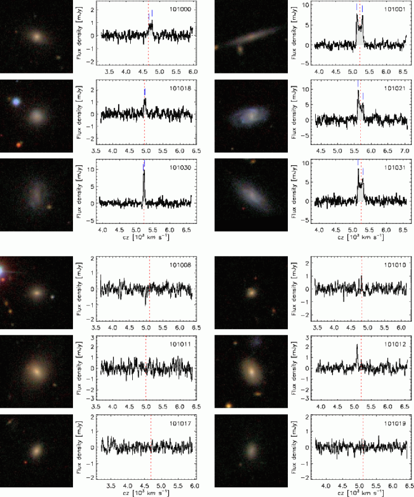
Figure A1: SDSS postage stamp images (1 arcmin square) and Hi-line profiles of GASS-low galaxies, ordered by increasing GASS number (indicated in each spectrum). Top three rows: Hi detections. The Hi spectra are calibrated, smoothed and baseline-subtracted. A dotted line and two dashes indicate the heliocentric velocity corresponding to the SDSS redshift and the two peaks used for width measurement, respectively. Bottom three rows: non-detections. This is a sample of the complete figure, which is available in the online version of the article.

Appendix B: Notes on Individual Objects

We list here notes for galaxies marked with an asterisk in the last column of Tables A2 and A3. The galaxies are ordered by increasing GASS number. In what follows, AA2 is the abbreviation for ALFALFA detection code 2.

Detections (Table A2)

101016 – asymmetric profile, uncertain width; confused with NGC 675 ($cz=5335$ km s^-1 from NED) $\sim$2.5 arcmin W; also notice large elliptical $\sim$1 arcmin W (NGC 677, 5082 km s^-1). Several small blue galaxies around, $z>0.08$.
101018 – polarization mismatch.
101021 – RFI spike at 1392 MHz ($\sim$6120 km s^-1); early-type galaxy $\sim$1 arcmin SE has $z=0.048$.
101030 – several galaxies within 3 arcmin, $z>0.06$.
107019 – small blue galaxy $\sim$1 arcmin W, $z=0.105$.
108011 – blue galaxy $\sim$1.5 arcmin SW, $z=0.052$.
108014 – blend with large, edge-on disk $\sim$2 arcmin SE (SDSS J081011.20+245334.7, $z=0.014056$); the face-on spiral $\sim$3 arcmin S haz $z=0.081$.
108019 – blend with blue companion $\sim$2 arcmin W (SDSS J081002.90+224623.1, $z=0.015736$, $cz=4718$ km s^-1).
108024 – confused/blend with two large spirals $\sim$1 arcmin NW (SDSS J082401.55+210138.3, $z=0.015483$) and $\sim$2.5 arcmin SW (SDSS J082355.28+205831.6, $z=0.015708$).
108029 – blend; interacting with large, blue companion 1.8 arcmin N (UGC 4264, $z=0.013642$).
108049 – AA2.
108051 – AA2.
108078 – small blue galaxy $\sim$1 arcmin W has no redshift; blue galaxy $\sim$1.5 arcmin S has $z=0.07$.
108093 – blue spiral $\sim$2 arcmin W, SDSS J083520.21+233943.2, has $z=0.039$.
108097 – small blue galaxy $\sim$3 arcmin W, $z=0.130$.
108129 – two small blue galaxies $\sim$2 arcmin W, $z>0.06$.
108140 – a few small galaxies within 3.5 arcmin, all in the background or without optical redshift; AA2.
108143 – face-on companion $\sim$2.5 arcmin N (SDSS J080037.51+134150.4, $z=0.01525$, $cz=4572$ km s^-1) not detected; blue galaxy $\sim$40 arcsec W, SDSS J080035.43+133936.8, has $z=0.073$.
108145 – polarization mismatch; high-frequency edge uncertain, systematic error. Companion $\sim$2 arcmin W (SDSS J080158.07+092324.2, $z=0.013337$, $cz=3998$ km s^-1) and two early-types $\sim$1.5 arcmin SE (SDSS J080210.94+092141.7, $cz=4795$ km s^-1) and $\sim$2 arcmin E (NGC 2511, $cz=4467$ km s^-1 from NED) not detected.
109009 – near bright star; AA2.
109020 – small blue galaxy $\sim$2 arcmin NE, $z=0.13$; AA2.
109034 – high-frequency edge uncertain, systematic error.
109058 – galaxy $\sim$2.5 arcmin SE has $z=0.132$.
109077 – AA2.
109079 – large, face-on blue companion $\sim$1.5 arcmin NE (UGC 5344, $cz$$\sim$4135 km s^-1) also detected.
109083 – AA2.
109094 – small blue galaxy $\sim$2.5 arcmin W, $z=0.012$.
109108 – AA2.
109120 – small galaxy $\sim$1.5 arcmin W, $z=0.09$; AA2.
109126 – AA2.
109129 – blend with blue companion $\sim$1 arcmin E (SDSS J090133.86+123931.6, $z=0.019761$).
109135 – AA2.
110013 – AA2.
110019 – galaxy $\sim$1.5 arcmin SW has $z=0.143$.
110038 – 264 mJy continuum source at 2 arcmin, but very strong signal.
110054 – blue, edge-on companion $\sim$3.5 arcmin SE (SDSS J104410.01+221233.2, $z=0.019602$), unlikely to contribute significantly to the signal; early-type galaxy $\sim$1 arcmin W has $z=0.110$.
110057 – blend with large, blue companion $\sim$2 arcmin NW (SDSS J102916.83+260557.2, $z=0.01699$).
110080 – two blue disks $\sim$2.5 arcmin NW and $\sim$2.5 arcmin N have redshifts $z=0.046$ and $z=0.162$, respectively.
111004 – blend with spectacular blue companion $\sim$3 arcmin E (SDSS J115805.22+275243.8, $z=0.011149$).
111047 – small blue galaxy $\sim$0.5 arcmin NE, no optical $z$.
110058 – blend with blue companion $\sim$3 arcmin N (SDSS J101823.53+131642.1, $z=0.018273$).
111053 – edge-on galaxy $\sim$2 arcmin NW, $z=0.067$.
111063 – polarization mismatch; large blue galaxy $\sim$4 arcmin NW (NGC 4005, $cz=4469$ km s^-1) not detected; blue disk $\sim$4 arcmin W (SDSS J115809.49+250520.0, $z=0.014286$, 4283 km s^-1), significant contamination unlikely.
111086 – blend with blue companion $\sim$3 arcmin N (SDSS J113913.53+150215.7, $z=0.014011$).
112035 – early-type companion $\sim$2 arcmin SE, SDSS J125910.30+273711.5 ($z=0.01916$, 5744 km s^-1); AA2.
112068 – high-frequency edge uncertain, systematic error. Large, red disk $\sim$1.5 arcmin NW (NGC 4063, $cz=4917$ km s^-1) not detected; disk $\sim$2.5 arcmin E has $z=0.024$.
112080 – blend: most of the Hi signal comes from large, blue companion $\sim$2 arcmin E (NGC 4615, $z=0.015731$ from NED); also notice spiral galaxy $\sim$3 arcmin S at the same redshift (SDSS J124131.46+260233.5, $z=0.015957$).
112014 – confused with face-on, blue companion $\sim$20 arcsec W (SDSS J120429.88+022654.5, $z=0.020141$, 6038 km s^-1); blue galaxy $\sim$2 arcmin W (SDSS J120424.60 +022732.8, $cz=6730$ km s^-1) not detected.
112112 – two small galaxies $\sim$1.5 and $\sim$2 arcmin NE, no $z$.
112116 – galaxies $\sim$1 arcmin SW and 2 arcmin S in the background ($z=0.021$ and $z=0.025$ respectively).
113010 – RFI spike at 1408 MHz ($\sim$2650 km s^-1).
113011 – disk galaxy $\sim$2.5 arcmin NE has $z=0.112$.
113038 – tiny blue comp. $\sim$2.5 arcmin SW, SDSS J132408.93+355317.6 ($z=0.018561$).
113091 – 3 small blue galaxies within 3 arcmin, $z>0.04$.
113115 – small blue galaxies $\sim$1.5 arcmin N and $\sim$3 arcmin SW in the background ($z>0.04$).
113118 – two galaxies $\sim$2.5 arcmin SW and $\sim$3 arcmin NW have $z=0.06$.
113122 – low-frequency edge uncertain, systematic error. Several galaxies within 3 arcmin, $z>0.05$.
113123 – blue disk galaxy $\sim$4 arcmin NE, $z=0.024$.
113124 – small blue galaxy $\sim$2 arcmin NE, $z=0.06$. Unclear what is causing the feature at 1398.5-99 MHz ($\sim$4600 km s^-1), but it is present in both polarizations.
114001 – small blue galaxy $\sim$45 arcsec W, no optical $z$.
114005 – confused/blend with blue companion $\sim$2 arcmin NW (IC 1013, $z=0.015341$, 4599 km s^-1); 3 large galaxies within 3 arcmin at the same redshift ($z=0.015$), and a smaller one 2 arcmin E ($z=0.013$).
114033 – blend with two large, blue companions $\sim$1 arcmin NE (SDSS J141216.00+155247.4, $z=0.017549$) and $\sim$2 arcmin SE (NGC 5504, $z=0.017505$ from NED).
114044 – profile edges uncertain, systematic error. Small blue galaxy $\sim$45 arcsec SW, no optical $z$.
114047 – blend/confused with blue triplet $\sim$2.5 arcmin E (SDSS J140520.30+102438.6, $z=0.018738$; SDSS J140519.91+102445.6, no $z$; SDSS J140520.30+102452.9, $z=0.018332$); also notice large early-type $\sim$2 arcmin E (SDSS J140516.52+102551.7, $z=0.017949$).
114076 – small blue galaxy $\sim$1.5 arcmin N, no $z$; AA2.
114077 – early-type galaxy $\sim$2 arcmin E, $z=0.030$; edge-on disk $\sim$0.5 arcmin W, no optical $z$.
114091 – large spiral $\sim$1.5 arcmin NE (UGC 9165, $cz=5259$ km s^-1 from NED) also detected; face-on spiral $\sim$2.5 arcmin SW has $z=0.079$. Absorption-like feature at $\sim$5050 km s^-1 is not RFI and is present in both polarizations (nothing obvious in the off position, just a few small blue galaxies without redshifts).
114110 – blend/confused with large blue companion $\sim$20 arcsec S, NGC 5491 ($z=0.019647$ from NED).
114115 – small blue galaxy $\sim$3.5 arcmin NE, $z=0.025$.
114144 – 120 mJy continuum source at 2 arcmin, standing waves. AA2.
122001 – two large galaxies $\sim$2 arcmin NE and 3 arcmin E have $z=0.037$; AA2.
122002 – strong signal detected on top of long standing wave (in polarization A).
124002 – AA2.
124012 – galaxy $\sim$1.5 arcmin NE, $z=0.15$; AA2.

Non-detections (Table A3)

101008 – blue disk $\sim$2 arcmin N has $z=0.034$.
101012 – detected companion ($cz=5080$ km s^-1), most likely the blue smudge $\sim$10 arcsec N (SDSS J014902.23+125603.2, no optical redshift).
108013 – galaxy $\sim$3 arcmin SW, SDSS J080229.78 +092743.2 ($z=0.014515$, 4351 km s^-1), also not detected.
108022 – blue companion $\sim$1 arcmin NW (SDSS J080206.54+092238.3, $z=0.013795$), also not detected.
108080 – blue disk galaxy $\sim$2 arcmin W has $z=0.047$.
108101 – perhaps hint of Hi galaxy signal.
108114 – blue companion $\sim$3.5 arcmin N (SDSS J081919.78+210331.8, $z=0.016114$), also not detected.
109022 – several galaxies within 3 arcmin, all in the background or without optical redshift.
109036 – AA2.
109064 – detected large spiral $\sim$2 arcmin S, (NGC 2874, $z=0.012573$, 3769 km s^-1); also notice large elliptical $\sim$2 arcmin SW, (NGC 2872, 3196 km s^-1 from NED).
109075 – low surface brightness galaxy $\sim$40 arcsec W, no optical $z$; 4 other galaxies within 3-4 arcmin, $z>0.06$.
109132 – detected blue, face-on companion $\sim$1.5 arcmin SE, SDSS J095905.12+102140.0 ($z=0.017938$, 5378 km s^-1).
110042 – several galaxies within 3 arcmin, all in the background or without optical redshift.
110047 – two galaxies within $\sim$1 arcmin E without optical $z$, probably in background.
110060 – large, early-type companion $\sim$3 arcmin S, SDSS J102058.56+253109.8 ($z=0.020785$, 6231 km s^-1), also not detected.
111024 – large, early-type companion $\sim$1.5 arcmin E, SDSS J114428.32+163329.1 ($z=0.011058$, 3315 km s^-1), also not detected.
111049 – detected blue companions $\sim$1.5 arcmin SW, SDSS J115752.02+250254.1 ($z=0.014196$, 4256 km s^-1) and $\sim$3 arcmin E, SDSS J115809.49+250520.0 ($z=0.014286$, 4283 km s^-1); also notice large spiral $\sim$4 arcmin NE, NGC 4005 (4464 km s^-1).
111066 – hint of Hi galaxy signal; blue face-on disk $\sim$2.5 arcmin SW has $z=0.085$.
112002 – galaxy $\sim$3 arcmin NE, SDSS J125806.06+272508.1 ($z=0.019237$, 5767 km s^-1) also not detected; galaxies $\sim$2.5 arcmin NE and $\sim$4 arcmin NW are in the background.
112003 – spiral galaxy $\sim$2 arcmin E has $z=0.025$; small galaxies $\sim$3 arcmin S also in background.
112004 – large disk $\sim$1 arcmin SW, SDSS J125746.16+274525.3 ($z=0.02051$, 6149 km s^-1) and small galaxy $\sim$2 arcmin SE, SDSS J125752.31+274422.7 ($z=0.023039$, 6907 km s^-1) also not detected; 4 other galaxies within 3 arcmin, $z>0.07$.
112011 – several galaxies within 3 arcmin, all in the background or without optical $z$.
112012 – galaxy $\sim$2.5 arcmin N has $z=0.023$.
112016 – perhaps hint of Hi galaxy signal (offset from SDSS redshift); small, blue companion $\sim$1.5 arcmin SW (SDSS J125317.61+262021.4, $z=0.02311$, 6928 km s^-1).
112017 – crowded field.
112060 – two nearby galaxies in background ($\sim$2 arcmin W, $z=0.025$ and $\sim$3 arcmin N, $z=0.026$).
112065 – perhaps hint of Hi signal (from galaxy and/or blue companion $\sim$3.5 arcmin SW, SDSS J120055.36+152221.8, $z=0.017482$, 5241 km s^-1).
112084 – detected face-on, blue companion $\sim$1.5 arcmin NW, SDSS J125905.29+273839.9 ($z=0.018117$, 5431 km s^-1); also notice smaller blue companion $\sim$2 arcmin SE (SDSS J125918.54+273536.9, $z=0.017777$, 5329 km s^-1) and galaxy $\sim$3 arcmin W (SDSS J125858.10+273540.9, $z=0.020057$, 6013 km s^-1), both not detected.
112089 – detected blue companion $\sim$1.5 arcmin NW, SDSS J125020.21+264459.4 ($z=0.02373$, 7114 km s^-1); perhaps hint of Hi signal from disk galaxy $\sim$1.5 arcmin S, SDSS J125026.59+264232.3 ($z=0.018702$, 5607 km s^-1).
112106 – detected large blue companion $\sim$1 arcmin NE (UGC 7035, $z=0.00409$) in board 4, $\sim$1414.5 MHz.
113001 – galaxy $\sim$1.5 arcmin NE, SDSS J130416.46+273022.9, has slightly higher redshift ($z=0.024$, $\sim$7200 km s^-1).
113004 – large face-on spiral $\sim$3 arcmin SE (SDSS J130126.12+275309.5, $z=0.018271$, 5478 km s^-1) and small galaxy $\sim$2 arcmin SW (SDSS J130104.82+275330.3, $z=0.019293$, 5784 km s^-1) also not detected.
113012 – over ten galaxies within 3 arcmin at slightly higher redshift ($z>0.018$).
113025 – four small galaxies within 1 arcmin, all without optical redshifts and most likely in the background.
113032 – early-type companion $\sim$3 arcmin SE, SDSS J130019.10+273313.3 ($z=0.019644$, 5889 km s^-1) also not detected; two galaxies $\sim$3 arcmin E and $\sim$2 arcmin W in background.
113040 – two galaxies within $\sim$1 arcmin E, $z>0.025$; blue smudge $\sim$20 arcsec S, no $z$.
113047 – companion $\sim$3 arcmin NW, SDSS J130010.41+273542.0 ($z=0.018676$, 5600 km s^-1); three galaxies between 1 and 3 arcmin SE, $z=0.024-0.026$.
113051 – four galaxies within $\sim$3 arcmin, $z=0.022-0.028$.
113060 – crowded field.
113078 – early-type $\sim$1 arcmin SW, SDSS J130231.87 +275607.9 ($z=0.022091$, 6623 km s^-1) also not detected.
113100 – hint of Hi galaxy signal; AA2. Three small galaxies 2-4 arcmin away, $z=0.02-0.025$.
113128 – crowded field.
114008 – marginally detected companion $\sim$1.7 arcmin W, GASS 114005 ($z=0.015153$, 4543 km s^-1; blend, see notes above); also notice SDSS J142807.22+255207.5 ($z=0.014591$, 4374 km s^-1) and NGC 5629 ($cz=4498$ km s^-1 from NED).
114025 – detected blue companion $\sim$2.5 arcmin E, SDSS J142532.21+254300.1 ($z=0.013609$, 4080 km s^-1); the disk galaxy $\sim$1 arcmin S of the blue companion has $z=0.075$.
114036 – blue companion 2.5 arcmin NE, SDSS J142758.85+255158.7 ($z=0.015341$, 4599 km s^-1), also not detected; notice two early-type galaxies $\sim$2 arcmin N ($z=0.014$) and $\sim$3 arcmin E ($z=0.015$).
114037 – detected companion, probably small blue galaxy $\sim$1.5 arcmin NW (SDSS J142829.10+272113.4, no $z$); NGC 5635 $\sim$4 arcmin N ($cz=4316$ km s^-1 from NED).
114038 – small galaxy 2 arcmin E, SDSS J142723.43 +255240.2 ($z=0.013418$, 4023 km s^-1).
114065 – early-type companion $\sim$2 arcmin W, SDSS J142714.65+255319.1 ($z=0.0159$, 4767 km s^-1).
114096 – a few galaxies between 2 and 3 arcmin in background, in particular SDSS J142544.50+254636.0, a blue galaxy 2 arcmin W ($z=0.075$) and SDSS J142600.40+254320.3, a large early-type $\sim$3 arcmin S ($z=0.076$ from NED).
123011 – three galaxies between 2 and 3 arcmin, $z>0.04$.

Table A1: SDSS and UV parameters of GASS-low galaxies

				log $M_{\star}$	$R_{50,z}$	$R_{50}$	$R_{90}$	log $\mu_{\star}$	extr	r	(b/a)r	incl	NUV$-r$	SFR
GASS	SDSS ID	Other name	$z_{\rm SDSS}$	(M⊙)	(″)	(″)	(″)	(M⊙ kpc-2)	(mag)	(mag)		(deg)	(mag)	(M⊙ yr-1)
(1)	(2)	(3)	(4)	(5)	(6)	(7)	(8)	(9)	(10)	(11)	(12)	(13)	(14)	(15)
124009	J000619.61+141938.7	–	0.0182	9.66	3.52	3.82	11.17	8.63	0.31	15.47	0.394	70	5.27	0.078
124012	J000629.29+141056.5	–	0.0178	9.74	6.03	6.72	16.28	8.27	0.34	15.79	0.144	90	4.26	0.162
124006	J001947.33+003526.8	–	0.0177	9.75	3.47	3.36	10.58	8.76	0.07	14.75	0.753	42	3.82	0.539
124004	J002534.40+005048.6	–	0.0178	9.31	5.35	6.11	11.54	7.93	0.06	15.32	0.917	24	2.21	0.326
124002	J004903.69+152907.9	–	0.0183	9.25	2.60	2.57	6.02	8.48	0.17	15.72	0.479	64	2.33	0.209
101021	J011653.58+000911.2	–	0.0190	9.22	4.22	5.03	11.03	8.00	0.09	15.49	0.686	48	2.21	0.276
101031	J014755.16+124131.0	–	0.0175	9.17	5.51	6.56	14.74	7.79	0.17	15.56	0.492	63	2.41	0.154
101030	J014803.60+125604.6	–	0.0175	9.10	7.06	8.85	17.38	7.50	0.18	15.99	0.659	50	2.90	0.061
101000	J014853.12+132526.2	–	0.0155	9.41	4.28	3.99	12.06	8.35	0.18	15.86	0.787	39	4.91	0.096
101012	J014902.52+125539.0	–	0.0174	9.83	3.77	4.01	9.92	8.78	0.22	15.06	0.642	52	5.17	0.027
101024	J014917.63+132759.9	–	0.0166	9.28	3.81	4.18	9.82	8.26	0.21	16.17	0.735	44	5.57	0.067
101016	J014918.93+130252.0	–	0.0178	9.72	2.53	2.74	6.50	8.99	0.24	15.53	0.845	33	5.51	0.007
101019	J014920.31+131754.5	–	0.0171	9.06	4.78	4.57	11.24	7.83	0.21	16.68	0.673	49	3.92	0.092
101011	J014933.52+131400.0	–	0.0167	9.95	4.66	4.96	14.21	8.75	0.20	14.84	0.768	41	5.92	0.013
101017	J014953.83+125833.7	–	0.0156	9.35	2.92	2.94	8.24	8.62	0.24	16.01	0.657	50	5.22	0.009

Note. – The full version of this table is available online.

Table A2: Hi Properties of GASS-low detections

			$T_{\rm on}$	$\Delta v$		$W_{50}$	$W_{50}^{c}$	$F_{\rm HI}$	rms		log $M_{\rm HI}$
GASS	SDSS ID	$z_{\rm SDSS}$	(min)	(km s-1)	$z$	(km s-1)	(km s-1)	(Jy km s-1)	(mJy)	S/N	(M⊙)	log $M_{\rm HI}$/$M_{\star}$	Q
(1)	(2)	(3)	(4)	(5)	(6)	(7)	(8)	(9)	(10)	(11)	(12)	(13)	(14)
124012	J000629.29+141056.5	0.0178	5	15	0.017 712	267$\pm$ 5	256	0.65$\pm$ 0.10	0.64	11.4	8.94	$-$0.81	1*
124004	J002534.40+005048.6	0.0178	5	12	0.017 816	130$\pm$ 2	122	0.71$\pm$ 0.07	0.72	17.5	8.99	$-$0.32	1
124002	J004903.69+152907.9	0.0183	4	12	0.018 269	205$\pm$ 3	195	0.67$\pm$ 0.11	0.90	10.6	8.98	$-$0.26	1*
101021	J011653.58+000911.2	0.0190	5	12	0.018 956	180$\pm$ 4	170	0.93$\pm$ 0.10	0.88	15.9	9.15	$-$0.06	1*
101031	J014755.16+124131.0	0.0175	5	12	0.017 465	173$\pm$ 3	164	0.86$\pm$ 0.07	0.67	19.7	9.05	$-$0.12	1
101030	J014803.60+125604.6	0.0175	10	10	0.017 445	44$\pm$ 1	39	0.42$\pm$ 0.03	0.57	25.0	8.74	$-$0.36	1*
101000	J014853.12+132526.2	0.0155	59	12	0.015 768	115$\pm$ 3	107	0.09$\pm$ 0.02	0.21	8.6	8.01	$-$1.40	1
101016	J014918.93+130252.0	0.0178	50	15	0.017 242	207$\pm$ 48	196	0.40$\pm$ 0.03	0.20	24.5	8.70	$-$1.01	5*
101001	J015032.27+133942.2	0.0174	10	12	0.017 372	202$\pm$ 5	193	1.10$\pm$ 0.07	0.56	27.9	9.15	$-$0.07	1
101018	J015036.88+130636.8	0.0165	59	12	0.016 531	69$\pm$ 7	62	0.07$\pm$ 0.02	0.24	7.5	7.94	$-$1.31	1*
107019	J074842.59+263223.2	0.0155	25	12	0.015 537	172$\pm$ 3	164	0.22$\pm$ 0.04	0.33	10.1	8.35	$-$0.81	1*
107026	J075433.01+294238.8	0.0167	5	10	0.016 672	223$\pm$ 3	215	3.58$\pm$ 0.11	1.02	53.3	9.63	$-$0.26	1
108143	J080038.05+133923.0	0.0158	23	12	0.015 754	101$\pm$ 7	94	0.26$\pm$ 0.04	0.51	10.3	8.45	$-$0.68	1*
108136	J080048.38+100500.9	0.0137	35	12	0.013 696	212$\pm$ 11	203	0.28$\pm$ 0.04	0.37	10.5	8.35	$-$1.12	1
108145	J080206.54+092238.3	0.0138	20	15	0.013 736	91$\pm$ 10	82	0.10$\pm$ 0.03	0.30	6.3	7.90	$-$1.26	2*

Note. – The full version of this table is available online.

Table A3: GASS-low non-detections

			$T_{\rm on}$	rms	log $M_{\rm HI}$,lim
GASS	SDSS ID	$z_{\rm SDSS}$	(min)	(mJy)	(M⊙)	log $M_{\rm HI}$,lim/$M_{\star}$	Note
(1)	(2)	(3)	(4)	(5)	(6)	(7)	(8)
124009	J000619.61+141938.7	0.0182	90	0.16	7.95	$-$1.70	…
124006	J001947.33+003526.8	0.0177	65	0.21	8.05	$-$1.71	…
101012	J014902.52+125539.0	0.0174	35	0.28	8.14	$-$1.68	*
101024	J014917.63+132759.9	0.0166	45	0.23	8.03	$-$1.25	…
101019	J014920.31+131754.5	0.0171	68	0.19	7.97	$-$1.09	…
101011	J014933.52+131400.0	0.0167	20	0.39	8.26	$-$1.69	…
101017	J014953.83+125833.7	0.0156	48	0.22	7.95	$-$1.40	…
101008	J014954.10+130735.9	0.0170	48	0.21	8.02	$-$1.33	*
101010	J015015.67+130826.8	0.0161	39	0.26	8.04	$-$1.13	…
108111	J080116.61+091553.3	0.0155	10	0.43	8.24	$-$1.72	…
108080	J080134.48+091817.4	0.0153	36	0.30	8.07	$-$1.25	*
108065	J080158.49+150331.5	0.0161	5	0.65	8.45	$-$1.65	…
108022	J080210.94+092141.8	0.0160	8	0.63	8.43	$-$1.61	*
108052	J080212.07+103234.1	0.0145	30	0.27	7.97	$-$1.63	…
108013	J080237.85+093000.3	0.0159	10	0.59	8.40	$-$1.69	*

Note. – The full version of this table is available online.

References

- Abazajian et al. (2009) Abazajian K. N. et al., 2009, ApJS, 182, 543
- Accurso et al. (2017) Accurso G. et al., 2017, MNRAS, 470, 4750
- Bahé et al. (2016) Bahé Y. M. et al., 2016, MNRAS, 456, 1115
- Baldry et al. (2012) Baldry I. K. et al., 2012, MNRAS, 421, 621
- Barnes et al. (2001) Barnes D. G. et al., 2001, MNRAS, 322, 486
- Bianchi, Conti & Shiao (2014) Bianchi L., Conti A., Shiao B., 2014, Advances in Space Research, 53, 900
- Bigiel et al. (2010) Bigiel F., Leroy A., Seibert M., Walter F., Blitz L., Thilker D., Madore B., 2010, ApJL, 720, L31
- Bigiel et al. (2008) Bigiel F., Leroy A., Walter F., Brinks E., de Blok W. J. G., Madore B., Thornley M. D., 2008, AJ, 136, 2846
- Binggeli, Sandage & Tammann (1985) Binggeli B., Sandage A., Tammann G. A., 1985, AJ, 90, 1681
- Blitz & Rosolowsky (2006) Blitz L., Rosolowsky E., 2006, ApJ, 650, 933
- Boselli, Cortese & Boquien (2014) Boselli A., Cortese L., Boquien M., 2014, A&A, 564, A65
- Boselli et al. (2014a) Boselli A., Cortese L., Boquien M., Boissier S., Catinella B., Gavazzi G., Lagos C., Saintonge A., 2014a, A&A, 564, A67
- Boselli et al. (2014b) Boselli A., Cortese L., Boquien M., Boissier S., Catinella B., Lagos C., Saintonge A., 2014b, A&A, 564, A66
- Boselli et al. (2010) Boselli A. et al., 2010, PASP, 122, 261
- Bothwell et al. (2014) Bothwell M. S. et al., 2014, MNRAS, 445, 2599
- Brinks (1990) Brinks E., 1990, in Astrophysics and Space Science Library, Vol. 161, The Interstellar Medium in Galaxies, Thronson Jr. H. A., Shull J. M., eds., pp. 39–65
- Brown et al. (2015) Brown T., Catinella B., Cortese L., Kilborn V., Haynes M. P., Giovanelli R., 2015, MNRAS, 452, 2479
- Brown et al. (2017) Brown T. et al., 2017, MNRAS, 466, 1275
- Catinella & Cortese (2015) Catinella B., Cortese L., 2015, MNRAS, 446, 3526
- Catinella, Haynes & Giovanelli (2007) Catinella B., Haynes M. P., Giovanelli R., 2007, AJ, 134, 334
- Catinella et al. (2012a) Catinella B. et al., 2012a, MNRAS, 420, 1959
- Catinella et al. (2013) Catinella B. et al., 2013, MNRAS, 436, 34
- Catinella et al. (2012b) Catinella B. et al., 2012b, A&A, 544, A65
- Catinella et al. (2010) Catinella B. et al., 2010, MNRAS, 403, 683
- Chabrier (2003) Chabrier G., 2003, PASP, 115, 763
- Cicone et al. (2017) Cicone C. et al., 2017, A&A, 604, A53
- Cortese et al. (2016) Cortese L. et al., 2016, MNRAS, 459, 3574
- Cox (2005) Cox D. P., 2005, ARA&A, 43, 337
- Davé et al. (2017) Davé R., Rafieferantsoa M. H., Thompson R. J., Hopkins P. F., 2017, MNRAS, 467, 115
- Davé, Thompson & Hopkins (2016) Davé R., Thompson R., Hopkins P. F., 2016, MNRAS, 462, 3265
- Dreyer (1888) Dreyer J. L. E., 1888, MmRAS, 49, 1
- Dreyer (1895) Dreyer J. L. E., 1895, MmRAS, 51, 185
- Dreyer (1908) Dreyer J. L. E., 1908, MmRAS, 59, 105
- Fu et al. (2010) Fu J., Guo Q., Kauffmann G., Krumholz M. R., 2010, MNRAS, 409, 515
- Fumagalli et al. (2009) Fumagalli M., Krumholz M. R., Prochaska J. X., Gavazzi G., Boselli A., 2009, ApJ, 697, 1811
- Giovanelli et al. (2005) Giovanelli R. et al., 2005, AJ, 130, 2598
- Glover & Clark (2012) Glover S. C. O., Clark P. C., 2012, MNRAS, 421, 9
- Gnedin & Kravtsov (2011) Gnedin N. Y., Kravtsov A. V., 2011, ApJ, 728, 88
- Haynes et al. (2011) Haynes M. P. et al., 2011, AJ, 142, 170
- Huang et al. (2012) Huang S., Haynes M. P., Giovanelli R., Brinchmann J., 2012, ApJ, 756, 113
- Janowiecki et al. (2017) Janowiecki S., Catinella B., Cortese L., Saintonge A., Brown T., Wang J., 2017, MNRAS, 466, 4795
- Kalberla & Kerp (2009) Kalberla P. M. W., Kerp J., 2009, ARA&A, 47, 27
- Kauffmann et al. (2012) Kauffmann G. et al., 2012, MNRAS, 422, 997
- Kennicutt & Evans (2012) Kennicutt R. C., Evans N. J., 2012, ARA&A, 50, 531
- Klessen & Glover (2016) Klessen R. S., Glover S. C. O., 2016, Star Formation in Galaxy Evolution: Connecting Numerical Models to Reality, Saas-Fee Advanced Course, Volume 43. ISBN 978-3-662-47889-9. Springer-Verlag Berlin Heidelberg, 2016, p. 85, 43, 85
- Krumholz (2013) Krumholz M. R., 2013, MNRAS, 436, 2747
- Krumholz, McKee & Tumlinson (2009) Krumholz M. R., McKee C. F., Tumlinson J., 2009, ApJ, 693, 216
- Lagos et al. (2014) Lagos C. D. P., Baugh C. M., Zwaan M. A., Lacey C. G., Gonzalez-Perez V., Power C., Swinbank A. M., van Kampen E., 2014, MNRAS, 440, 920
- Lagos et al. (2015) Lagos C. d. P. et al., 2015, MNRAS, 452, 3815
- Leroy et al. (2008) Leroy A. K., Walter F., Brinks E., Bigiel F., de Blok W. J. G., Madore B., Thornley M. D., 2008, AJ, 136, 2782
- Lilly et al. (2013) Lilly S. J., Carollo C. M., Pipino A., Renzini A., Peng Y., 2013, ApJ, 772, 119
- Martig et al. (2009) Martig M., Bournaud F., Teyssier R., Dekel A., 2009, ApJ, 707, 250
- Martin et al. (2005) Martin D. C. et al., 2005, ApJL, 619, L1
- McKee & Ostriker (1977) McKee C. F., Ostriker J. P., 1977, ApJ, 218, 148
- Meyer et al. (2017) Meyer M., Robotham A., Obreschkow D., Westmeier T., Duffy A., Staveley-Smith L., 2017, PASA, 34
- Meyer et al. (2004) Meyer M. J. et al., 2004, MNRAS, 350, 1195
- Moffett et al. (2016) Moffett A. J. et al., 2016, MNRAS, 457, 1308
- Nilson (1973) Nilson P., 1973, Uppsala general catalogue of galaxies
- Obreschkow et al. (2009) Obreschkow D., Heywood I., Klöckner H.-R., Rawlings S., 2009, ApJ, 702, 1321
- Popping, Behroozi & Peeples (2015) Popping G., Behroozi P. S., Peeples M. S., 2015, MNRAS, 449, 477
- Popping, Somerville & Trager (2014) Popping G., Somerville R. S., Trager S. C., 2014, MNRAS, 442, 2398
- Rahmati et al. (2013) Rahmati A., Schaye J., Pawlik A. H., Raičevic M., 2013, MNRAS, 431, 2261
- Saintonge (2007) Saintonge A., 2007, AJ, 133, 2087
- Saintonge et al. (2016) Saintonge A. et al., 2016, MNRAS, 462, 1749
- Saintonge et al. (2017) Saintonge A. et al., 2017, ApJS, 233, 22
- Saintonge et al. (2011) Saintonge A. et al., 2011, MNRAS, 415, 32
- Saintonge et al. (2012) Saintonge A. et al., 2012, ApJ, 758, 73
- Schaye et al. (2015) Schaye J. et al., 2015, MNRAS, 446, 521
- Seibert et al. (2012) Seibert M. et al., 2012, in American Astronomical Society Meeting Abstracts, Vol. 219, American Astronomical Society Meeting Abstracts #219, p. 340.01
- Serra et al. (2012) Serra P. et al., 2012, MNRAS, 422, 1835
- Springob et al. (2005) Springob C. M., Haynes M. P., Giovanelli R., Kent B. R., 2005, ApJS, 160, 149
- Stevens & Brown (2017) Stevens A. R. H., Brown T., 2017, MNRAS, 471, 447
- Wang et al. (2011) Wang J. et al., 2011, MNRAS, 412, 1081
- Wolfire et al. (1995) Wolfire M. G., Hollenbach D., McKee C. F., Tielens A. G. G. M., Bakes E. L. O., 1995, ApJ, 443, 152
- Wong et al. (2006) Wong O. I. et al., 2006, MNRAS, 371, 1855
- Wright et al. (2010) Wright E. L. et al., 2010, AJ, 140, 1868
- Wyder et al. (2007) Wyder T. K. et al., 2007, ApJS, 173, 293
- Yang et al. (2007) Yang X., Mo H. J., van den Bosch F. C., Pasquali A., Li C., Barden M., 2007, ApJ, 671, 153
- Young et al. (1995) Young J. S. et al., 1995, ApJS, 98, 219
- Young et al. (2011) Young L. M. et al., 2011, MNRAS, 414, 940
- Zoldan et al. (2017) Zoldan A., De Lucia G., Xie L., Fontanot F., Hirschmann M., 2017, MNRAS, 465, 2236
- Zwicky et al. (1961) Zwicky F., Herzog E., Wild P., Karpowicz M., Kowal C. T., 1961, Catalogue of galaxies and of clusters of galaxies, Vol. I