Large-deviation Properties of Linear-programming Computational Hardness of the Vertex Cover Problem
Abstract
The distribution of the computational cost of linear-programming (LP) relaxation for vertex cover problems on Erdös-Rényi random graphs is evaluated by using the rare-event sampling method. As a large-deviation property, differences of the distribution for “easy” and “hard” problems are found reflecting the hardness of approximation by LP relaxation. In particular, by evaluating the total variation distance between conditional distributions with respect to the hardness, it is suggested that those distributions are almost indistinguishable in the replica symmetric (RS) phase while they asymptotically differ in the replica symmetry breaking (RSB) phase. In addition, we seek for a relation to graph structure by investigating a similarity to bipartite graphs, which exhibits a quantitative difference between the RS and RSB phase. These results indicate the nontrivial relation of the typical computational cost of LP relaxation to the RS-RSB phase transition as present in the spin-glass theory of models on the corresponding random graph structure.
I Introduction
In statistical mechanics, combinatorial optimization problems have attracted a great deal of attention during the past two decades phase-transitions2005 ; 26 ; moore2011 . The motivation and hope is to obtain an understanding of the source of computational hardness which is inherent to many combinatorial optimization problems papadimitriou1998 . The statistical mechanics approaches are based on taking a physics perspective and applying notions and techniques from the the field of disordered systems like spin glasses. Actually, from the computer science point of view, understanding the computational hardness is still lacking. This is visible from the fact that the famous P–NP problem garey1979 is still not solved. Here, P is a class of “easy” problems that can be solved in the worst case in polynomial time and NP contains the problems for which the solution can only be checked in polynomial time. So far, for no problem in NP, an algorithm is known which finds solutions of the problems in worst case in polynomial time. On the other hand, it is not proved that no such algorithm will exist.
In contrast to the worst-case analysis, one is often interested in the typical case running time, in particular for real-world applications. From a fundamental science point of view, by studying the properties of given easy and hard samples, one might be able to understand the source of computational complexity. For this reason, in statistical mechanics one started to investigate random ensembles of NP-hard problems, which are typically controlled by one or several parameters. Examples are satisfiability problems with random formulas, the traveling salesperson problems for randomly distributed cities, or the vertex-cover (VC) problems on random graphs. For these ensembles phase transitions have been observed at the boundary between a phase where the random instances are typically easy to solve and another phase where the random instances are typically hard. mitchell1992 ; monasson1997 ; mertens1998 ; wh1 ; phase-transitions2005 .
Interestingly, the actually hardest instances are often found right at the phase transitions. This reminds the statistical physicist on the critical slowing down which appears, e.g., for the Monte Carlo simulation of the ferromagnetic Ising model. Thus, to understand the source of computational hardness best, it might be beneficial to study the hardest instances available, e.g., the problem instances which are located right at the phase transitions. As an alternative approach, some attempts have been performed to construct hard instances guided by physical insight horie1996 ; hoos2000 ; liu2015 ; jia2007 . Examples are instances designed such that equivalent spin-glass instances exhibit no bias in the distributions of local fields and exhibit a first order transition with a backbone satsat2002 or such that, due to the degeneracy, many existing solutions of an optimization problem are isolated zdeborova2006 . Recently, a heuristic algorithm has been implemented marshall2016 to automatically construct spin-glass instances with respect to finding the ground state as hard as possible (for a given ground-state algorithm). We extend this approach in the present work by sampling instances of an optimization problem in equilibrium, the hardness (i.e., the number of steps of the optimization algorithm) is interpreted as the “energy” of the instance. The sampling is controlled by an artificial temperature. In particular our approach allows us, in addition to obtain very hard instances, to obtain the distribution of the hardness over the random problem ensemble, even down to the low-probability tails. One tail will contain very hard instances, the other tail very easy instances. Such large-deviation approaches have been applied, e.g., to study the distribution of scores of random-sequence alignment AKH2002 , the distribution of the size of the largest components of random graphs AKH2011 , the distribution of endpoints of fractional Brownian motion fBm_MC2013 , or the distribution of non-equilibrium work work_ising2014 . This fairly general approach enables us to investigate how the shape of the hardness distribution changes as a function of the control parameter. In particular we can investigate how the distribution differs in the phases where the typically easy and the typically hard instances are found, respectively.
In particular, we study the VC problem on the Erdős-Rényi random graphs erdoes1960 with average connectivity as a control parameter. Here, the easy-hard transition was observed wh1 at ( is the Euler’s number). This transition was independent of the algorithm used, branch-and-bound with leaf removal Tak or linear programming (LP) with cutting-plane approach dh . Analytically, the replica symmetry (RS) is broken at as well wh1 . These past studies have been performed by studying typical instances for different values of . To our knowledge, nobody has studied full distribution of the “computational hardness,” measured in a suitable way, for this problem. Also for the other NP-hard problems we are not aware of such studies. Here, we use a linear-programming relaxation to solve VC. Nevertheless, only obtaining the full distribution of the quantities of interest allows the full understanding of any random problem. In particular, the tails of the distribution contain the very easy and very hard instances. Studying the properties of those hardest possible instances might allow to get better understanding of the source of the computational hardness.
The reminder of the paper is organized as follows: Next, we define the VC problem formally and state the linear-programming algorithm which we applied for solving the VC problem. In the third section, we explain the large deviation approach used to obtain the distribution of hardness. In section four we present our results. We close the paper by a summary and a discussion of our results.
II Vertex covers and LP relaxation
In this section, we define minimum vertex-cover (min-VC) problems and introduce LP relaxation as an approximation scheme.
Let be an undirected graph with a vertex set and an edge set . It is assumed that does not have multi-edges nor self-loops. A set is called vertex cover of if any edge connects to at least a vertex in . A vertex in vertex cover is called covered. The (unweighted) min-VC problems is then defined as a computational problem to search a vertex cover with the minimum number of covered vertices. For a mathematical formulation, we set a binary variable to each vertex , which takes one if vertex is covered and zero otherwise. The problem is then represented as an integer programming (IP) problem as follows:
| (1) |
Min-VCs belong to a class of NP-hard garey1979 indicating that no exact algorithm is known that can solve the problem in the worst case in polynomial time as a function of problem size . To avoid this computational hardness, approximation algorithms are commonly used. Especially, the linear programming relaxation is a fundamental approximation scheme for the IP problems. For LP relaxation, constraints on binary variables, , are replaced to continuous constraints with interval . Thus, the LP-relaxed min-VC problem is represented by
| (2) |
It is a kind of LP problems which can be exactly solved in polynomial time using an ellipsoid method Kha . However, since it is computationally costly, other exact algorithms such as Dantzig’s simplex method and the interior-point method Kar are often used. Their difference lies in the strategy to search an optimal solution on a facet of the simplex defined by constraints in Eq. (2); the former moves from an extreme point to another extreme point at each step but the latter can search feasible solutions inside the simplex. Note that if a solution of the relaxed problem contains only integer variables, it is, by minimality, automatically a solution of the corresponding IP problem. The fact enables us to naively define the hardness of the min-VC problems for LP relaxation by counting the number of non-integer values in an LP-relaxed solution. It is worth noting that VC problems have a good property called half integrality; considering extreme-point solutions of the problem, they are represented by vectors with half integers, nt . Thus, for VC, all non-integer values are .
One of our goals in this paper is to investigate the relationship between the structure of min-VCs on random graphs and its statistical-mechanical picture by using LP relaxation. To achieve the goal, we mainly examine the computational cost of the simplex method hopefully reflecting the structure of the simplex given by Eq. (2). Since it restricts candidates of optimal solutions to feasible solutions lying on extreme points of the polytope, the computational cost, i.e., the number of iterations reaching to the optimal solution, is regarded as a measure of complexity of the simplex solver and of the problem. For the simplex method, there are some solvers and a number of initialization schemes and pivot rules which may change the computational cost to treat a given instanced by the algorithm, respectively. As described later, however, our main findings are independent of those selections.
Before closing this section, we describe how the random graphs are defined for which we obtain min-VCs. In this paper, we examine Erdős-Rényi (ER) random graphs as a random ensemble. Each instance of such a random graph is generated by, starting with an empty graph, creating an ?undirected edge for each pair of vertices with probability , i.e., connecting the two nodes. Here represents average degree. Then, the degree distribution converges to the Poisson distribution with mean as the number of vertices grows. As described in the previous section, it has been revealed that the randomized problems exhibit a phase transition related to RS and its breaking (RSB) at wh1 , which is also the threshold where LP relaxation fails to approximate the problems with high accuracy dh ; th2 . While the relation is usually observed for other ensembles th4 , the ER random graph is the simplest example to investigate the graph structure making the problem hard for LP relaxation.
III Rare-event sampling
As we consider min-VCs on an ensemble of random graphs, it is necessary to estimate distributions of observables over those instances. The rare-event sampling is useful to estimate distributions over a large range of the support even into the tails because it significantly reduces the number of samples needed compared to a simple sampling. Depending on the application, probabilities as small as or smaller are easily accessible. In computational physics, the task is crucial for various fields and some sampling schemes such as the Wang-Landau method WL and multicanonical method berg ; IH have been developed, which were originally used to sample configurations with extreme energies in the Boltzmann ensemble. Nevertheless, instead of the energy the sampling can be with respect to any measurable quantity AKH2002 . This and similar approaches are, e.g., widely used for estimating large-deviation properties of random graph structures AKH2015 ; AKH2017 ; AKH2017_2 .
Now we briefly describe the outline of the estimation. In this paper, we estimate the distribution of number of iterations of an simplex solver for LP-relaxed min-VCs for ER random graphs. Since is considered as a function of a graph , we need to sample graphs following the weight of the ER random graphs with the number of vertices fixed. For an unbiased sampling, each graph follows the distribution given by
| (3) |
where , , and is a set of graphs with cardinality . A biased sampling with respect to is then executed by sampling graphs with the following distribution:
| (4) |
where represents a “temperature” of the system, which can also be negative, and the partition function is given by
| (5) |
In practical simulations practical_guide2015 , the choice of the temperature determines the range of the values of where the sampling of graphs is concentrated. Please notice that the unbiased sampling corresponds to the limit in Eq. (4).
The reweighting method is used to obtain the distribution of over a large range of the support. The distribution reads
| (6) |
where represents a Kronecker delta. Biased distribution with temperature is represented by
| (7) |
This indicates that the unbiased distribution can be estimated by using the relation,
| (8) |
The factor is estimated by comparing sampled to estimated . Naturally, this will work only if there is an overlap in the actually sampled ranges of the support for from unbiased sampling and . This allows already to extend the range of the support where is known. Therefore, can be obtained for additional temperatures by starting at a sufficiently high temperature, allowing to extend the range of the support even more, again and again, where each time is calculated with respect to the so-far known .
Practically, the biased samplings are executed by the Markov Chain Monte-Carlo (MC) method. A graph is represented by a sequence with length which contains random numbers in . For each pair of nodes, iff the random number is below , an edge connects the two nodes. is obtained as the number of iterations of a simplex solver which solves Eq. (2) for . To construct the Markov chain of the sequences, we used the Metropolis-Hastings algorithm, which is based on generating trial sequences and accepting them with a certain probability. To construct a trial sequence is copied from the current and then 0.5% of randomly chosen elements in are changed. The corresponding graph is generated as explained above. Next, is obtained. Finally, is accepted, i.e., becomes the new current sequence in the Markov chain, according to the Metropolis-Hastings acceptance probability which reads
| (9) |
Otherwise is rejected, i.e., is kept.
For a biased sampling, one should validate whether the system is equilibrated. It is a simple way to check sufficient relaxation of observables from different initial conditions. Fig. 1 shows an example of relaxation of two observables, the number of LP iterations and average degree of each sampled graphs. In the simulations, the number of vertices and the average degree of ER random graphs is fixed. Graphs are sampled according to Eq. (9) with from three different initial graphs, the null graph, the complete graph, and a graph simply sampled from ER random graphs. We find that they merge up to 3500 MC trials and then fluctuate similarly around an equilibrim value indicating that relaxation is promptly realized 111Usually, the number of updates in the MC sampling is counted by MC steps, the number of trials divided by a system size. In this paper, we instead use the number of updates itself because of the running time per update and the relatively short relaxation time..
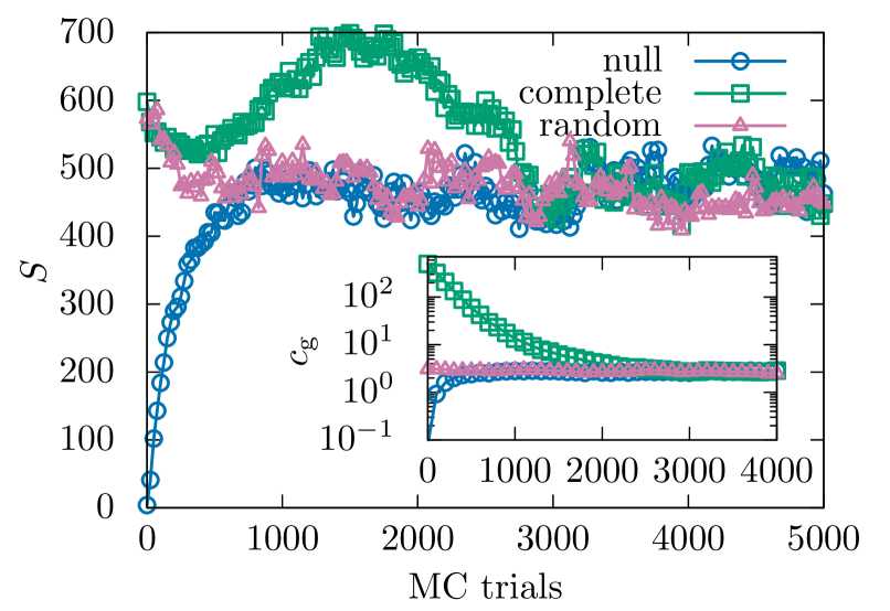
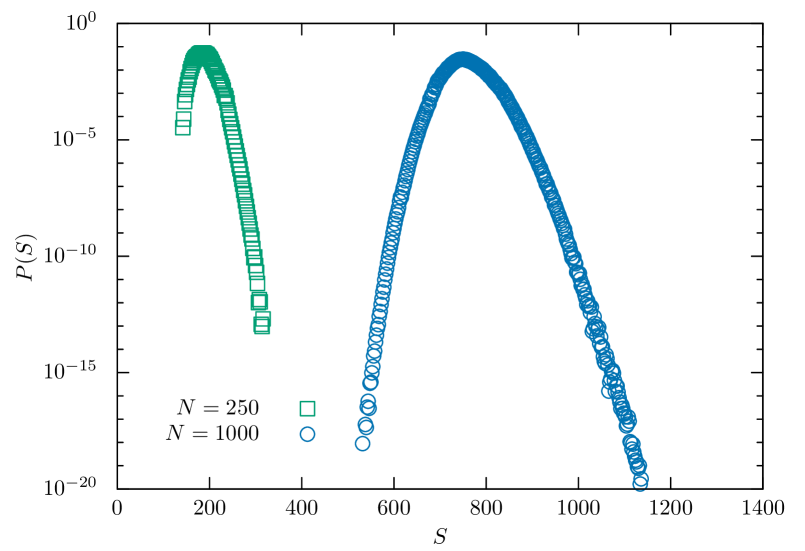
Fig. 2 shows the estimated distribution of LP iterations for ER random graphs with for and . As a simplex LP solver, lp_solve is used with default settings. Note that we here, for the moment, do not distinguish between instances which are optimally solved, i.e., all variables are zero or one, and those instances which are not optimized, i.e., where some variables are half-integer valued. The distribution is generated from an unbiased sampling and biased sampling with different temperatures , and . Those samplings are executed for MC trials and the first observations are omitted to ignore nonequibilium states for biased ones. The figure shows that the tails of distributions are evaluated up to in spite of executing trials per a sampling.
IV Results
In this section, we describe the main results. First, to evaluate the asymptotic behavior of the distributions of the number of LP iterations, an empirical rate function is introduced. Next, to reveal a relation to the RS-RSB transition, we define hardness of approximation for an instance and evaluate the distance between conditional distributions with respect to the hardness. Its asymptotic behavior suggests a quantitative difference of the distance between the RS and RSB phase. Lastly, since VC on bipartite graphs can be solved in polynomial time, we investigate a quantity defined as the similarity to bipartite graphs and its relation to the hardness.
IV.1 Empirical rate functions
As indicated in Fig. 2, the estimated distributions themselves are not suitable for comparison. To visualize their finite-size effects, both axes should be rescaled. For the number of LP iterations , its average over random graphs with vertices is used for a linear regression given by
| (10) |
Then, the number of LP iterations is rescaled by . In our simulations, the order is close to one while it has been theoretically unrevealed.
For the distribution , we introduce an empirical rate function which reads
| (11) |
where represents the rescaled number of LP iterations. In the large-deviation theory denHollander2009 ; Tou , one says that the large-deviation principle holds if, loosely speaking, the empirical rate function converges for to a limiting rate function function . Thus, in this case it represents the asymptotic behavior of tails of a distribution as follows:
| (12) |
The empirical rate function thus indicates finite-size effects including terms. Due to the logarithm and taking to obtain , the normalization and the subleading term of become for finite values of an additive contribution, which converges to zero for if the large-deviation principle holds.
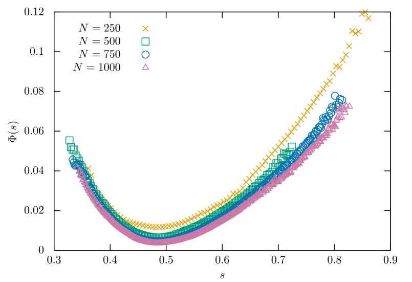
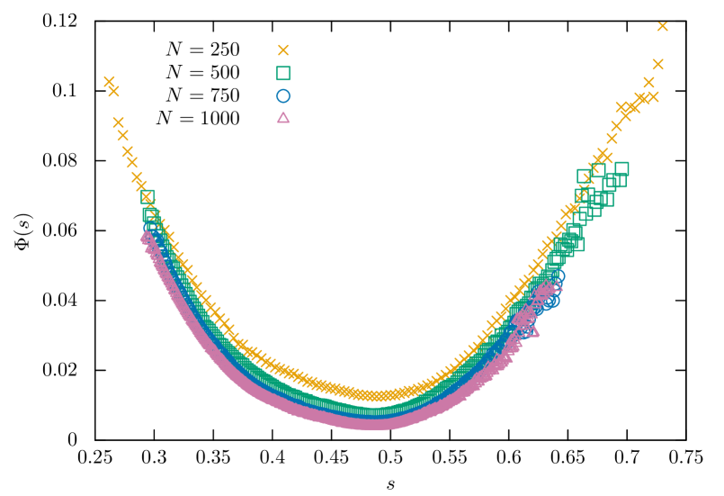
Fig. 3 shows the empirical rate functions for ER random graphs with average degree , i.e., in the RS phase, whose distributions are displayed in Fig. 2. As grows, the position on the -axis of the minimum and also the full shape of the function seem to approach to a common position and a common shape, respectively. This convergence indicates that the large deviation principle may hold for the rate function of the number of LP iterations. Since these empirical rate functions are not symmetric with respect to their peaks, the distribution of LP iterations differs from a simple Gaussian distribution. In Fig. 4, we show empirical rate functions in the case where , i.e., in the RSB phase. Compared to Fig. 3, a change on the left-hand side of the functions is clearly observed. This comparison indicates that the distributions of LP iterations might exhibit a qualitative difference related to the RS-RSB phase transition.
IV.2 Distance of distributions conditioned by hardness of problems
As described in the last section, a naive expectation is that the computational cost of a simplex LP solver is correlated to the hardness of LP relaxation for a problem. We introduce conditional distributions of LP iterations with respect to the hardness of problems to validate the expectation.
For numerical evaluation in this subsection, an alternative LP solver called CPLEX is executed while the results are qualitatively same as the case of lp_solve. The reason is the scalability of CPLEX; it is more than a hundred times as fast as lp_solve, which enables us to set the large number of MC trials up to and the large size of graphs up to . We use the rare-event sampling method in the last section with biased samplings at temperatures , and in addition to unbiased samplings.
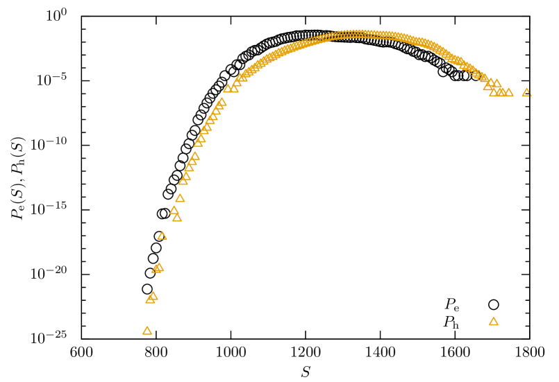
As described in the last section, an instance is considered hard to obtain the optimal solution if the LP-relaxed solution contains at least a half integer. Correspondingly, conditional distributions and are respectively defined by distributions of LP iterations over easy and hard instances, respectively. Fig. 5 shows an example of these distributions for ER random graphs with and . The figure suggests that the expectation about correlation between the number of LP iterations and the hardness of problems is correct because two distributions are separated. The separation is also observed in the case of lp_solve resulting in the difference of distributions in Fig. 3 and 4.
Using conditional distributions, we specifically examine the “distance” of those distributions. Since two sampled distributions generally have different supports, the often used Kullback–Leibler distance diverges, for example. A total variation distance is an alternative distance which stays finite even in the case of two distributions with completely different supports. The total variation distance between distributions and is defined by
| (13) |
where is the union of supports of two distributions. Unlike the Kullback–Leibler divergence, the total variation distance is a kind of metric. Since , it always lies in the interval and, especially, takes zero iff equals to as a distribution.
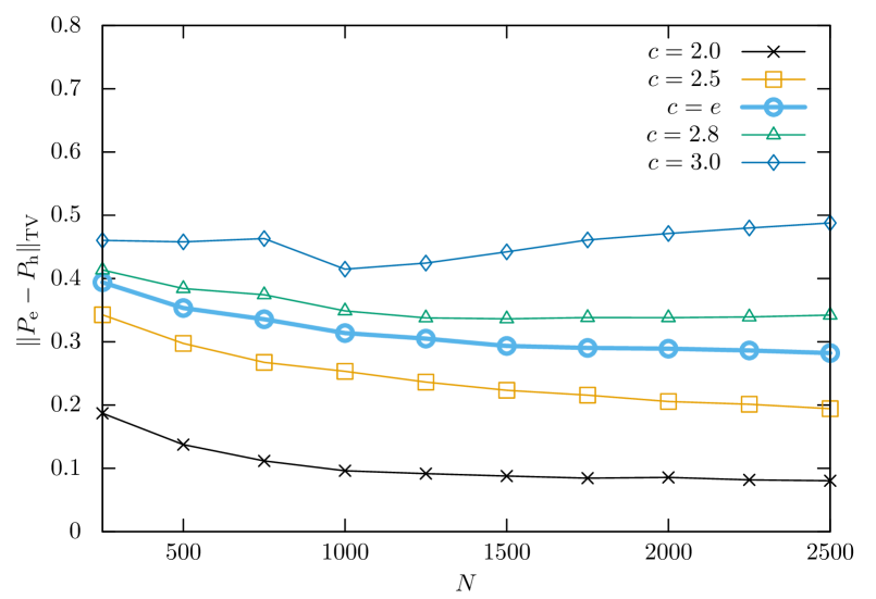
Fig. 6 shows the finite-size dependence of the total variation distance between conditional distributions and for ER random graphs with various average degree around the transition value . Note that for values outside this interval, it turned out to be hard to obtain sufficient statistics for both easy and hard instances at the same time, even with the large-deviation approach. In the RS phase where , it decreases monotonously and converges nearly to zero. It implies that here the LP computational cost varies almost independently to the hardness of LP-relaxed min-VCs in the large- limit. On the other hand, for , the distance of two distributions remains positive even for large and seems even to grow, when looking at the data. The fact suggests that the computational cost of the simplex method strongly depends on the hardness of instances in the RSB phase. Asymptotic behaviors of conditional distributions result in the difference of the empirical rate functions in Fig. 3 and Fig. 4.
IV.3 Relation to graph structure: bipartiteness
In this subsection, we study a graph invariant and investigate a possible relation to the computational cost of a simplex solver. In particular, we introduce “bipartiteness” as to which extend a given graph resembles a bipartite graph. A bipartite graph is a graph for which the set of nodes can be partitioned into two subsets such that there are only edges which connect one node from one subset to a node from the other subset. Therefore, there are no edges which connect nodes within one subset alone.
In mathematical optimization, Kőnig’s theorem is a fundamental result that min-VC problems on bipartite graphs can be solved exactly in polynomial time Kon . In ER random graphs, the fact suggests that almost every instances are easy to solve with high accuracy under the percolation threshold, i.e., , where a graph consists in trees which are always bipartite and contain only short cycles with length . Note that Kőnig’s theorem relates the min-VC to the maximum perfect matching, which can be found in polynomial time, but we deal with LP here. Nevertheless, it therefore does not come as a full surprise that LP for the relaxed problem finds optimal solutions for original min-VC for .
In contrast, the random graphs are typically not bipartite above the percolation threshold because of the emergence of a loopy giant component. However, as we will see below, the still existing closeness to bipartite graphs allows even for to see some correlation between the bipartiteness and the number of LP iterations.
Before describing the numerical results, we define bipartiteness as the fraction of edges in a maximum cut (max-cut). A cut of graph is a partition of vertex set into and . Then, a cut set is defined as a set of edges connecting to each vertex subset and , i.e., . The maximum cut of is a cut with the largest number of edges among possible cuts. The fraction of edges of a max-cut is then defined as
| (14) |
It is an indicator of bipartiteness because it equals one iff a graph is bipartite. Since solving a max-cut problem belongs to the class of NP-hard problems, we restricted ourself to calculate approximately. In our numerical simulations, it is approximated by the following greedy procedure:
-
(i)
add each vertex to either of two sets with probability ,
-
(ii)
choose an augmenting vertex named such that the number of neighboring vertices in the same subset is less than that of neighboring vertices in the other subset,
-
(iii)
move from the current subset to the other subset,
-
(iv)
if there exists an augmenting vertex, return to (iii) or stop otherwise.
The algorithm finally finds a locally optimal solution in that it is the best solution among all cut sets by adding or by deleting a vertex. We found that in practice, this algorithm is executed in typically iterations for a sampled graph.
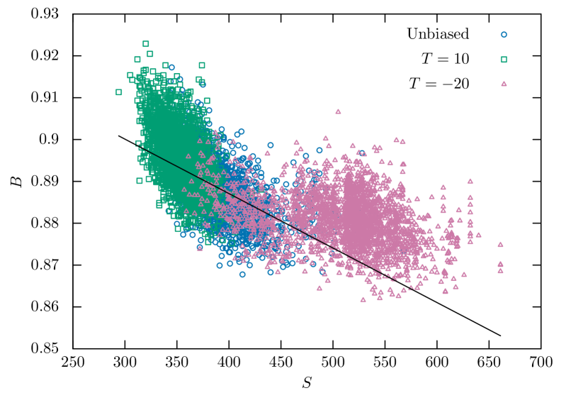
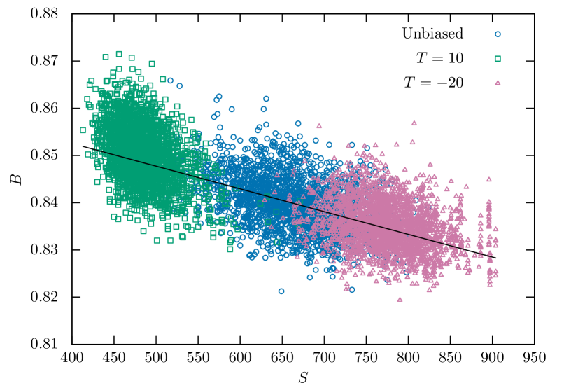
We are interested in the question whether there exists a correlation between the bipartiteness and the number of LP iterations to find a solution. We first show scatter plots of and sampled from ER random graphs with and with (Fig. 7) and (Fig. 8). In those plots, biased samplings with different temperatures and are executed in addition to unbiased samplings. We find that, regardless of RS and RSB phases, and have a strong negative correlation. However, such a correlation may result almost trivially from a fluctuation of the number of edges in ER random graphs: as the number of edges increases, also increases because in general graphs with a higher value of are harder to solve. On the other hand should decrease for a higher number of edges, because for small values of almost all graphs are collections of trees, which are completely bipartite, while densely connected graphs are not bipartite. To omit such a spurious correlation, it is necessary to consider an ensemble of random graphs, where the number of edges is fixed to . In the thermodynamic limit , both ensembles agree erdoes1960 .
Now we concentrate on the estimation of correlation between and for ER random graphs with the number of edges fixed. The correlation is calculated as the Pearson correlation coefficient defined by
| (15) |
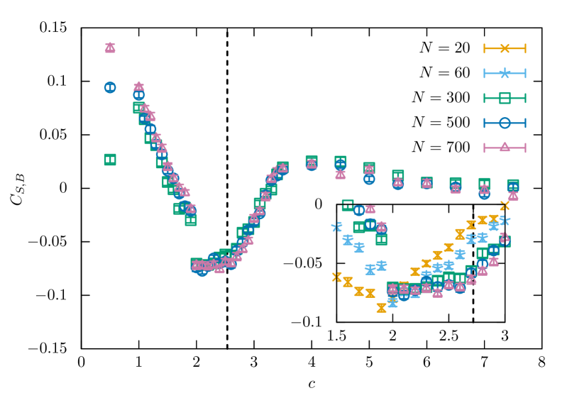
where represents an average over sampled graphs. Fig. 9 shows the correlation coefficient estimated by unbiased samplings with graphs whose number of edges is fixed to . CPLEX is used as a simplex solver again. The standard deviation of is estimated by the bootstrap method. Namely, the data are uniformly resampled and a correspondent is calculated for 50 times to estimate its standard deviation. As shown in Fig. 9, it is found that the finite size effect looks small for above the percolation threshold , since the data points fall on top of each other for different values of . In the case of , the sampled data shapes just a point in the scatter plot because all sampled graphs are nearly bipartite. It makes an accurate estimation of difficult. Above the percolation threshold, gradually decreases and becomes negative above . The gap of between and emerges because of an intrinsic behavior of the solver. It must be emphasized, however, that relatively strong negative correlations are observed below the RS–RSB threshold and the correlation moves nearly to zero above the threshold regardless of a simplex solver.
In summary, even though a trivial correlation related to the number of edges is omitted, we find a relatively weak but characteristic behavior of the correlation coefficient between the number of LP iteration and bipartiteness . Consequently, the intuition that similarity to bipartite graphs decreases the computational cost of a simplex LP solver is (slightly) correct only in the RS phase where the majority of graphs in the ensemble is easy to obtain optimal solutions. Note that we have studied also other graph invariants such as a Becchi number and degree correlations to seek for a correlation to the number of LP iterations. So far, we did not find such a correlation for any value of .
V Summary and Discussions
In this paper, we numerically investigate the large-deviation properties of computational cost for LP relaxation and relations to a phase transition in the spin-glass theory and to random graph structure. The rare-event sampling is executed to efficiently examine the large-deviation properties. It enables us to estimate the tails of the distributions efficiently illustrating its asymmetric property and finite-size effects. Furthermore, we naively introduce the hardness of LP relaxation and evaluate the total variation distance between conditional distributions with respect to the hardness. Numerical results show that the distance asymptotically becomes very small for while it remains larger and seems even to grow with graph size otherwise. It is indicated that conditional distributions are asymptotically distinguishable in the RSB phase, which reflects the hardness of instances for LP relaxation. The results are compatible to the differences observed in the empirical rate functions. Finally, the relation of computational cost of LP relaxation to graph structure is studied. We specifically examine bipartiteness of graphs defined as the fraction of edges in the maximum cut. It is suggested that it is weakly but negatively correlated to the number of LP iterations in the RS phase though they are nearly uncorrelated otherwise.
The rare-event sampling based on the reweighting method helps us to find a valid signature in the distribution in this paper. To access the further details of the tail of the distribution, a biased sampling with lower temperature can be performed in principle. It is observed, however, that the system with negatively low temperature, e.g., , is hard to equilibrate using the Metropolis-Hastings algorithm. It could be beneficial to use another rare-event sampling scheme such as the Wang-Landau method or an advanced MC sampling method like the replica exchange MC method 91 .
As for the relation to graph structure, we find a valid negative correlation to the computational cost of LP relaxation in the RS phase though it vanishes in the RSB phase. A possible reason of the uncorrelated result for is the hardness of estimating the bipartiteness in the region. In fact, the max-cut problem on the ER random graphs corresponding to finding the ground energy of the antiferromagnetic spin-glass model ZB also exhibits the RS-RSB transition at average degree . It suggests that the greedy procedure in the last subsection fails to find the optimal fraction of max-cut even though it is executed repeatedly. While the large part of graph invariants is hard to compute exactly, we have to leave it to a future work to find even better one to characterize the complexity of graph structure even in the RSB phase.
In the view of the spin-glass theory, it is considered that local structures called frustrations evoke the RSB phase 26 . For Ising spin glasses on a finite dimensional lattice, for example, there is an attempt to detect the transition point using frustrated plaquettes, i.e., frustrated shortest loops in the lattice Miya ; Ohz . In the case of a spin-glass model on a sparse random graph, however, it is not straightforward to define such a local structure because graph invariants describe rather global structure. A long range frustration Zhou1 based on the cavity method is a strong candidate though it is difficult to evaluate numerically in practice. It is thus an important task to find another measure of frustrations in random graphs to predict the hardness of each instance. The result in this paper suggests that the LP relaxation is possibly useful to investigate the measure numerically by evaluating the correlation to the computational cost of a solver.
Evaluating the typical computational cost of a LP solver over randomized problems by analytical approaches is highly challenging though the worst-case computational cost has been a central issue of mathematical optimization. Our study on the large-deviation properties shows the existence of the common properties irrelevant to the details of solvers and of nontrivial relations to the phase transition, the spin-glass picture, and random graph structures. We believe that numerical analyses in this paper stimulate the further progress in understanding typical behavior of LP relaxation for randomized optimization problems and its vast relationships to other concepts including the spin-glass theory.
Acknowledgements.
The use of IBM ILOG CPLEX has been supported by the IBM Academic Initiative. This research is partially supported by JSPS KAKENHI Grant Nos. 25120010 (KH) and 15J09001 (ST).References
- (1) A. K. Hartmann and M. Weigt, Phase Transitions in Combinatorial Optimization Problems, (Wiley-VCH, Weinheim ,2005).
- (2) M. Mézard and A. Montanari, Information, Physics, and Computation (Oxford University Press, Oxford, 2009).
- (3) C. Moore and S. Mertens, The Nature of Computation, (Oxford University Press, Oxford, 2011).
- (4) C. Papadimitriou and K. Steiglitz, Combinatorial Optimization – Algorithms and Complexity, (Dover Publications Inc., Mineola, NY, 1998).
- (5) M. R. Garey and D. S. Johnson, Computers and Intractability, (Freeman, San Francisco, 1979).
- (6) D. Mitchell, B. Selman, and H. Levesque, in Proceedings of the AAAI-92, 459 (1992).
- (7) R. Monasson and R. Zecchina, Phys. Rev. E 56, 1357 (1997).
- (8) S. Mertens, Phys. Rev. Lett. 81, 4281 (1998).
- (9) M. Weigt and A. K. Hartmann, Phys. Rev. Lett. 84, 6118 (2000).
- (10) A. Horie and O. Watanabe, Lect. Notes Comput. Sci. 1350, 22 (1996).
- (11) H. Hoos and T. Stützle, J. Autom. Reasoning 24, 421 (2000).
- (12) R. Liu, W. Luo, and L. Yue, Data Knowl. Engin. 100, 1-18 (2015).
- (13) H. Jia, C. Moore and D. Strain, J. Artif. Intell. Res. 28, 107-118 (2007).
- (14) W. Barthel, A. K. Hartmann, M. Leone, F. Ricci-Tersenghi, M. Weigt, and R. Zecchina, Phys. Rev. Lett. 88, 188701 (2002).
- (15) L. Zdeborova and Marc Mézard, J. Stat. Mech.2006, P12004 (2006).
- (16) J. Marshall, V. Martin-Mayor, and I. Hen, Phys. Rev. A 94, 1 (2016).
- (17) A. K. Hartmann, Phys. Rev. E, 65, 056102 (2002).
- (18) A. K. Hartmann, Eur. Phys. J. B, 84, 627 (2011).
- (19) A. K. Hartmann, S. N. Majumdar, and A. Rosso, Phys. Rev. E, 88, 022119 (2013).
- (20) A. K. Hartmann, Phys. Rev. E 89, 052103 (2014).
- (21) P. Erdős and A. Rényi, Publ. Math. Inst. Hungar. Acad. Sci. 5, 17–61 (1960).
- (22) J. Takahashi, S. Takabe, and K. Hukushima, J. Phys. Soc. Jpn. 86, 073001 (2017).
- (23) T. Dewenter and A. K. Hartmann, Phys. Rev. E 86, 041128 (2012).
- (24) L. G. Khachiyan, USSR Comput. Math. Math. Phys. 20, 53 (1980).
- (25) N. Karmarkar, Proc. of the sixteenth annual ACM symp. on Theo. of comp. 302 (1984).
- (26) G. L. Nemhauser and L. E. Trotter Jr., Math. Program. 6, 48 (1974).
- (27) S. Takabe and K. Hukushima, J. Phys. Soc. Jpn. 83, 043801 (2014).
- (28) S. Takabe and K. Hukushima, J. Stat. Mech. 2016, 113401 (2016).
- (29) F. Wang and D. P. Landau, Phys. Rev. Lett. 86, 2050 (2001).
- (30) B. A. Berg and T. Celik: Phys. Rev. Lett. 69, 2292 (1992).
- (31) Y. Iba and K. Hukushima, J. Phys. Soc. Jpn. 77, 103801 (2008).
- (32) T. Dewenter and A. K. Hartmann, New J. Phys. 17, 015005 (2015).
- (33) A. K. Hartmann, Eur. Phys. J. Spec. Top. 226, 567 (2017).
- (34) A. K. Hartmann and M. Mézard, arXiv:1710.05680 (2017).
- (35) A. K. Hartmann, Big Practical Guide to Computer Simulations, (World Scientific, Singapore, 2015)
- (36) F. den Hollander, Large Deviations, (American Mathematical Society, Providence, 2000)
- (37) H. Touchette, Phys. Rep., 478, 1 (2009).
- (38) D. König, Matematikai és Fizikai Lapok, 38, 116 (1931).
- (39) K. Hukushima and K. Nemoto, J. Phys. Soc. Jpn. 65, 1604 (1996).
- (40) L. Zdeborová and S. Boettcher, J. Stat. Mech. 2010, 02020 (2010).
- (41) R. Miyazaki, J. Phys. Soc. Jpn. 82, 094001 (2013).
- (42) M. Ohzeki, Y. Kudo, and K. Tanaka, J. Phys. Soc. Jpn. 87, 015001 (2017).
- (43) H. Zhou, Phys. Rev. Lett. 94, 217203 (2005).