An unexpected detection of bifurcated blue straggler sequences in the young globular cluster NGC 2173

Abstract

Bifurcated patterns of blue straggler stars in their color–magnitude diagrams have atracted significant attention. This type of special (but rare) pattern of two distinct blue straggler sequences is commonly interpreted as evidence of cluster core-collapse-driven stellar collisions as an efficient formation mechanism. Here, we report the detection of a bifurcated blue straggler distribution in a young Large Magellanic Cloud cluster, NGC 2173. Because of the cluster’s low central stellar number density and its young age, dynamical analysis shows that stellar collisions alone cannot explain the observed blue straggler stars. Therefore, binary evolution is instead the most viable explanation of the origin of these blue straggler stars. However, the reason why binary evolution would render the color–magnitude distribution of blue straggler stars bifurcated remains unclear.

1. Introduction

Blue straggler stars (BSSs) are commonly found in old globular clusters (GCs), which are generally characterized by ages in excess of $\sim$10 Gyr, and in Galactic open clusters (OCs) of various ages (e.g., Ferraro et al., 2003; Xin & Deng, 2005; Mathieu & Geller, 2009; Li et al., 2013; Baldwin et al., 2016). They appear to be main-sequence (MS) stars that are significantly more massive than the cluster’s bulk population (Sandage, 1953; Stryker, 1993). In star clusters, BSSs usually occupy a region that is bluer and brighter than the MS turnoff (MSTO) in the Hertzsprung–Russell diagram or its observational equivalent, the color–magnitude diagram (CMD). They tend to have an upper limit $\sim$2.5 magnitudes brighter than the MSTO. Blue straggler stars are thought to be produced either by direct stellar collisions (Hills & Day, 1976) or through the evolution of binary systems, e.g., through mass transfer or stellar mergers (McCrea, 1964; Andronov et al., 2006). Direct stellar collisions can also involve binary–binary or binary–single star interactions (Fregeau et al., 2004), or interactions of triple stars through the Kozai mechanism (e.g., Perets & Fabrycky, 2009). We encourage readers to explore Boffin et al. (2015) for more details regarding our current understanding of BSSs.

The relative importance of direct stellar collisions versus binary evolution in old GCs remains an open question. Nevertheless, it has been suggested that the dominant BSS formation channel may be through binary evolution, irrespective of the host cluster’s dynamical state (Knigge et al., 2009). Without going through some special dynamical processes, BSSs formed through any of the possible formation channels would be expected to exhibit a featureless distribution beyond the MSTO of their host cluster. However, observations of two distinct BSS populations featuring similar numbers of stars in the CMDs of a number of old Galactic GCs offer evidence in support of the notion that stellar collisions could be of comparable importance (Ferraro et al., 2009; Dalessandro et al., 2013; Simunovic et al., 2014). Numerical simulations have shown that zero-age collisional BSSs would lie on a locus that is clearly bluer than that defined by the BSSs formed through binary mass transfer, thus implying that the blue-sequence stars are likely products of stellar collisions (e.g., Ferraro et al., 2009). However, because the formation rate of collisional BSSs depends on the local stellar number density, only clusters that are sufficiently old and dense could produce sufficient numbers of collisional BSSs along a cluster’s MS extension (Davies et al., 2004). Indeed, so far three GCs have been detected that show a bifurcation in their BSS populations, two of which exhibit cusps in their radial number-density profiles (Ferraro et al., 2009; Dalessandro et al., 2013), a feature expected to result from core collapse (Cohn, 1980; Lynden-Bell & Eggleton, 1980). The only exception is the GC NGC 1261. Although it does not show evidence of a cusp in its radial number-density profile, it has nevertheless been claimed to be in a post-core-collapse state (Simunovic et al., 2014). Therefore, all of these features observed in these old GCs may imply that the frequent stellar collisions that produce the blue-branch stars were driven by core-collapse events.

In this article, we report the unexpected detection of a bifurcated BSS distribution in the Large Magellanic Cloud (LMC) cluster NGC 2173, which is much younger and which has a much lower central stellar mass density than the old GCs exhibiting bifurcated BSS populations. This is the first detection of a bifurcated distribution of BSSs in a cluster that is much younger than the old GCs. Dynamical calculations carried out for this cluster show that stellar collisions are unlikely responsible for the observed BSSs; therefore, binary evolution may indeed be the only viable scenario. However, why BSSs formed through binary evolution would form a bifurcated distribution in a cluster’s CMD remains an open question.

This article is organized as follows. Section 2 includes the details of the observations and the data reduction. In Section 3 we present our main results, which we briefly discuss in Section 4. Section 5 provides a summary of the main results and our conclusions.

2. Data Reduction

2.1. Photometry and Data Processing

The cluster NGC 2173 was observed with the Hubble Space Telescope (HST) using the Wide Field Camera 3/Ultraviolet and Visual Channel (WFC3/UVIS) as part of program GO-12257 (PI: L. Girardi). The observations of NGC 2173 were obtained through the F336W and F814W filters, with total exposure times of 1980 s and 1520 s, respectively. For the observations in both filters, we used the WFC3 module of the dolphot2.0 package to perform point-spread-function (PSF) photometry on the flat-fielded data frames (referred to as ‘_flt’). dolphot2.0 automatically calculates a sky map and combines observations with short and long exposure times into a final stellar catalog.

We processed the raw stellar catalog as follows. We first selected all detected objects flagged as ‘good stars’ by dolphot2.0. Next, we adopted a filter employing a sharpness constraint based on the sharpness parameter calculated by dolphot2.0, which enabled us to remove unusually concentrated objects (such as cosmic rays) or extended sources (such as background galaxies). A perfect star should have a sharpness equal to zero. We only selected objects with $-0.2<$ sharpness $<0.2$ in both frames. The ‘crowding’ parameter quantifies how much brighter an object would have been had nearby stars not been fitted simultaneously (it is expressed in units of magnitudes). We further only selected objects with crowding $\leq 0.5$ mag in both frames. Because the positions of the BSSs in the CMD are very different from those expected for cosmic rays or extended sources, while they are also very bright, we confirmed that our data reduction process would not remove any of detected BSS candidates.

We estimated the differential reddening suffered by each star by application of the method proposed by Milone et al. (2012). We found that the reddening variations across the full observational field of NGC 2173 range from $E(B-V)=-0.03$ mag to 0.09 mag. The resulting reddening-corrected CMD does not show any significant differences compared with the original CMD. In Fig. 1 we present the raw CMD (left panel), as well as the processed CMD of the entire image of NGC 2173. The bifurcated BSS populations are obvious in both CMDs.

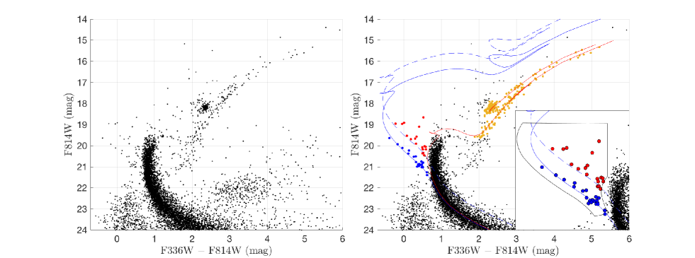
Figure 1.— Unprocessed (left) and final (right) CMDs of NGC 2173. Blue, red circles: blue, red-branch BSSs; orange circles: selected RGB, RC, and AGB stars. The red and blue solid lines are best-fitting isochrones with ages of $\log{(t\mbox{ yr}^{-1})}=9.20$ and 8.40, respectively. The blue dashed line is the locus of the equal-mass binary sequence corresponding to the young isochrone. The inset in the right-hand panel highlights the region used for selecting BSSs. (Stellar catalogs behind this figure are online accessible.)

2.2. Isochrone Fitting

We used the PARSEC isochrones (Bressan et al., 2012) to fit our observations. We used two isochrones to fit the bulk of the cluster population and the BSSs, respectively. For the bulk stars, we adopted an age of $\log{(t\mbox{ yr}^{-1})}=9.20$ (1.58 Gyr), a metallicity of $Z=0.008$, an extinction of $A_{V}=0.155$ mag, and a distance modulus of $(m-M)_{0}=18.40$ mag. Because of the small number of BSSs and the lack of an apparent MSTO region, adopting a precise age for the BSSs is difficult. We forced the isochrone to fit the brightest blue-branch BSS. This leads to an adopted (maximum) age of $\log{(t\mbox{ yr}^{-1})}=8.40$ (250 Myr). Fig. 1 shows that the brightest blue-branch BSS is very close to the zero-age MS (ZAMS), which means that any isochrone with an age younger than 250 Myr would be able to adequately represent these blue-branch stars. The adopted age of 250 Myr is therefore simply an upper limit. Our adopted best-fitting parameters for the bulk of the cluster’s stellar population are close or identical to those of Grocholski et al. (2007) and Milone et al. (2009). The best-fitting isochrones are shown in the right-hand panel of Fig. 1. The red-branch BSSs are characterized by a lower boundary which is close to the locus of the equal-mass binary sequence. One can easily separate the two BSS branches through visual inspection, as shown in the right-hand panel of Fig. 1 (insets).

2.3. Determinations of the Different Stellar Samples

We selected BSSs as follows: (a) their magnitudes cover the range $18.0\leq m_{\rm F814W}\leq 21.5$ mag; (b) they are brighter than the 250 Myr-old isochrone plus 0.1 mag in the F814W filter (on average, this is the 3$\sigma$ level defined by the photometric uncertainties); (c) they are bluer than the 1.58 Gyr-old isochrone minus 0.15 mag in ($m_{\rm F336W}-m_{\rm F814W}$), corresponding to, on average, the 3$\sigma$ color uncertainty level. The total number of selected BSSs is 40.

As shown in Fig. 1, the BSSs in NGC 2173 exhibit a clear bifurcation in the cluster’s CMD. For each BSS, we calculated its relative distance to the 250 Myr-old isochrone, as well as to the corresponding equal-mass MS–MS binary locus. BSSs which were located closer to the isochrone for single stars were assigned to the blue sequence (see the blue circles in Fig. 1), while those closer to the equal-mass binary locus were included in our red-sequence sample (the blue circles in Fig. 1).

We also selected a sample containing most red-giant branch (RGB), red clump (RC), and asymptotic giant branch (AGB) stars. We first identified the position of the bottom of the RGB in the CMD. Stars brighter than this position and located in the 3$\sigma$ region bracketing the isochrone were selected as sample stars (see the orange circles in Fig. 1).

2.4. Artificial Star Tests

Some artificial effects, like line-of-sight blending of two stars or the diffraction spikes of bright giant stars, may mimic a broadened or even a split BSS population. To inspect if any of our BSSs might have been affected by the spikes of bright stars, we examined their ‘roundness’ parameter calculated by dolphot2.0. A perfect star should have a roundness of zero. If an object is extended or has been affected by diffraction spikes, its roundness will be significantly larger than that for ‘good’ stars. The largest roundness value for our BSSs is 0.265, which is smaller than the equivalent values for 80% of all detected objects; 39 of the 40 observed BSSs have roundness values below 0.103, which is better than the values for 90% of all detected objects. We additionally explored the importance of these effects globally through artificial star tests. The principle of this method consists of generating a large number of artificial stars characterized by the same PSF as the observational data, adding them to the raw data image, and then using the same approach as for the sample of real stars to recover them. By comparing their output CMD to the corresponding input diagram, we can evaluate how artificial effects (including photometric uncertainties) change the morphology of the original color–magnitude distribution.

To do this, we generated two different artificial star samples composed of artificial stars characterized by an initial color–magnitude distribution defined by the 250 Myr and 1.58 Gyr-old isochrones, both with a Kroupa-like mass function (Kroupa, 2001). To optimize our calculation time, for the young artificial stellar sample we only generated stars that were brighter than $m_{\rm F814W}\leq 23$ mag, because the bottom morphology of its MS is almost identical to that of the old artificial stars. Our young and old artificial stellar samples contained 70,000 and 700,000 stars, respectively. Their spatial distributions were homogeneous. To avoid a situation in which the artificial stars dominate the background and crowding levels, we only added 100 artificial stars to the raw image at any one time. This means that for the young and old artificial stellar samples, we repeated this procedure 700 and 7000 times, respectively.

We present the output CMDs of both the young and old artificial stars in the left-hand panel of Fig. 2. We found that the recovered color–magnitude diagram shows a MS of roughly the same width as the real MS, as well as a broadened region toward the red side of the MS. The latter is caused by stellar blending. We specifically investigated the output CMDs of both regions for BSSs and RGB, RC, and AGB stars, as shown in the top and bottom right-hand panels of Fig. 2. We did not find any bifurcated patterns in these regions. Our detection of bifurcated BSS populations is therefore unlikely caused by artificial effects.

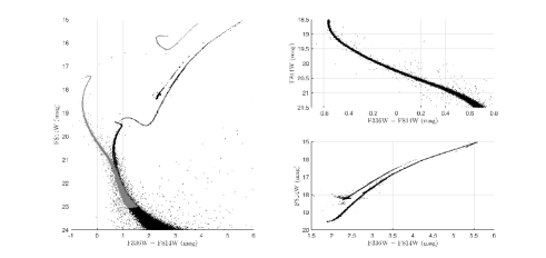
Figure 2.— (Left) Output CMDs of the young (grey) and old (black) artificial stellar samples. (Top right) Output CMD of the young artificial stars with the same magnitude range as the observed BSSs. (Bottom right) Output CMD of the artificial RGB, RC, and AGB stars. To optimize image space, we only exhibit a fraction of our artificial stars.

The artificial stellar catalog also allowed us to derive a stellar completeness map. Artificial stars that meet the criteria below are considered stars that would contribute to the sample’s incompleteness:

1. Stars that do not return any photometric result.

2. Stars not defined as a ‘good’ star by Dolohot2.0.

3. Stars with crowding parameter $>0.5$ mag.

4. Stars with sharpness parameter $<-0.2$ or $>0.2$.

The completeness levels will be used to correct the derived stellar number-density profile, as well as any radial distributions of the numbers for different stellar samples.

2.5. Determination of the Cluster’s Global Parameters

To determine the coordinates of the cluster center, we generated number-density contours for the cluster and determined the coordinates where the local number densities reached the largest values. We adopted the latter as the cluster’s center. The resulting center coordinates are $\alpha_{\rm J2000}=-5^{\rm h}57^{\rm m}58.32^{\rm s}$ and $\delta_{\rm J2000}=-72^{\circ}58^{\prime}44.40^{\prime\prime}$. The left-hand panel of Fig. 3 presents the spatial stellar distribution, the number-density contours, and the resulting cluster center. We realize that blending affects the number-density level at different positions, especially in the cluster’s central region. In the right-hand panel of Fig. 3, we compare the position derived for the cluster center with the completeness map. The cluster center is indeed located in a region of relatively low stellar completeness, indicating that our derived center position is reliable. In addition, our center coordinates are very close to those adopted by Baumgardt et al. (2013).

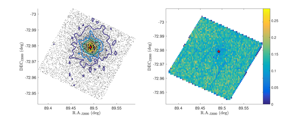
Figure 3.— (Left) Spatial stellar distribution in the observed field of NGC 2173. The red pentagram represents the cluster center. Number-density contours have been superimposed. (Right) Completeness map, with completeness levels indicated by the color bar, for all artificial stars.

The stellar completeness map shown in the right-hand panel of Fig. 3 shows a very low level of completeness ($<30$%). This is expected, because we have generated an artificial stellar sample that contains a large number of low-mass stars (based on the Kroupa mass function adopted). Almost all of these low-mass (and thus faint) stars cannot be detected. If we were to constrain the stellar sample to the range $m_{\rm F814W}\leq 24$ mag, the overall completeness would be higher than 90%.

After obtaining the cluster center and sample completeness levels, we calculated the stellar number-density profile using all detected stars with $m_{\rm F814W}\leq 24$ mag. We first used the cluster center to define annular rings with intervals of 1 pc. The stellar number density in each ring is the ratio of the observed number of stars in the ring and the ring’s area, corrected for the level of incompleteness,

$$\rho(r)=\frac{N(r)}{f(r)A(r)},$$ (1)

where $N(r)$ is the number of stars in the ring at radius $r$, $f(r)$ is the corresponding completeness in the ring, and $A(r)$ is the ring’s area.

The stellar completeness as a function of radius, as well as the resulting number-density profile, are shown in Fig. 4. We next used the empirical King model (King, 1962) and a constant background field population, $b$, to fit their profiles,

$$\rho(r)=k\left[\frac{1}{\sqrt{1+(r/r_{\rm c})^{2}}}-\frac{1}{\sqrt{1+(r_{\rm t}/r_{\rm c})^{2}}}\right]+{b},$$ (2)

where $r_{\rm c}$ and $r_{\rm t}$ are the core- and tidal radii, respectively. If we assume that the background stars are homogeneously distributed across the entire image, then $b$ is a constant which represents the number density of the background; $k$ is a normalization coefficient. Our best-fitting core- and tidal radii are $r_{\rm c}=2.67$ pc and $r_{\rm t}=131.30$ pc, respectively. Because of the small HST/WFC3 field, the full image actually only includes about a quarter of the cluster’s tidal radius; the maximum cluster radius covered is only $\sim$32 pc. Based on the best-fitting King model, we also derived the radius that contains half the number of stars, i.e., $r_{\rm h}=9.75$ pc. Our result is consistent with that derived by McLaughlin & van der Marel (2005).

The commonly adopted approach to subtract the field stellar contribution involves selecting a nearby region as reference field, followed by randomly removing a similar color–magnitude distribution from the observed cluster+field CMD as that covered by the field stars only. However, the large size of NGC 2173 and the small size of the observed field cause problems in this regard. We cannot properly account for the effects of field-star contamination based on the cluster’s CMD. Indeed, as we already showed in Fig. 1, the bifurcated pattern of BSSs is already obvious in the raw CMD of the entire observed region. Field stars of different ages and metallicities are very unlikely to give rise to such a feature, however. In this article, we did not subtract any ‘field’ stars from the observed CMD. Instead, we statistically evaluated the contributions of field stars at different radii. We defined the cluster member probability of each star as the ratio of the local densities of the star cluster and the background field,

$$P(r)=\frac{\rho(r)-b}{\rho(r)}.$$ (3)

The profile of the cluster membership probability is presented in the bottom panel of Fig. 4. As expected, a large fraction of the image is actually dominated by cluster stars. We found that for radii $r\leq 16.65$ pc, the observed numbers of stars are dominated by the cluster ($P\geq 50$%). Below, we will specifically limit our study to BSSs found within this radius.

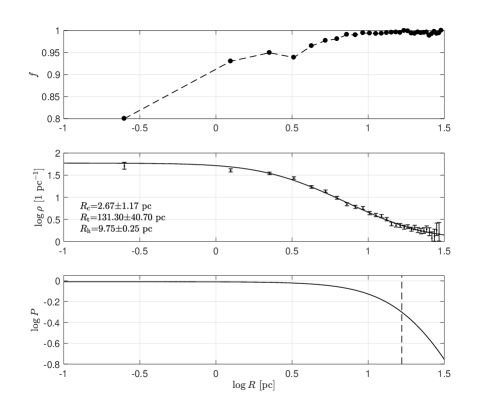
Figure 4.— (Top) Stellar completeness as a function of radius. (Middle) Stellar number-density profile and best-fitting King model. (Bottom) Estimated cluster membership probability as a function of radius.

3. Main Results

3.1. Significance

As shown in the right-hand panel of Fig. 1, the bifurcated BSS pattern in the CMD of the NGC 2173 field is indeed obvious. The numbers of the red- and blue-branch stars are comparable, with 18 of them belonging to the red branch and 22 associated with the blue branch. We first evaluate the tightness of our blue- and red-branch BSSs by comparing their color-magnitude distributions to the best fitting isochrone (or the equal-mass binary sequence for red-branch BSSs). We calculate the color deviation for each blue- and red-branch stars to the best fitting isochrone (equal-mass binary sequence). We found the distribution of color deviations for blue-branch BSSs can be well described by a Gaussion function, with a standard deviation of $\Delta_{\rm c}$=0.060$\pm$0.033 mag, which is consistent with the typical photometric error for BSSs $\Delta_{\rm c}$=0.041$\pm$0.002 mag, the latter is determined from the CMD of artificial stars. This means the blue-branch BSSs can be well explained by a population of single stars with photometric errors. In contrast, the distribution of color deviations for red-branch BSSs cannot be described by a Gaussion distribution. To further quantify the dispersion of red-branch stars, we calculate the root-mean-square (RMS) of their color deviations, we found the RMS of red-branch BSSs is more than three times that of blue-branch BSSs (0.23 mag vs. 0.07 mag). In summary, the blue-branch BSSs are well associated with the best fitting isochrone. The red-branch BSSs are more dispersed than the blue-branch BSSs.

We then investigate the significance of the bifurcated pattern of BSSs, to do this we generated a synthetic stellar sample with an age of 250 Myr located in the BSS region. For each of them, we randomly assigned a binary component associated with the 1.58 Gyr-old stellar population, with the relevant mass ratio selected randomly from zero to unity. All these binary systems are unresolved in our simulation. The synthetic CMD is shown in the left-hand panel of Fig. 5, where the mass ratios are indicated by the color bar.

Intriguingly enough, unlike the binary sequence below the MSTO region, the high mass-ratio binary sequence in the BSS region is not parallel to the ZAMS. The binaries are significantly dispersed toward the red, which is similar to the observed red-branch BSSs. The reason for unparalleled high mass-ratio binary sequences is because the secondary stars associated with these high mass-ratio binary systems have already evolved off the MS (or may be ready to leave the MS), therefore these binary systems are no longer MS-MS binaries.

We divided both the observed and synthetic samples into three parts (see the black dashed lines in Fig. 5) which roughly define the regions for the blue- and red-branch stars, and the middle gap. In our adoption, only one BSS is located between these two lines. We then randomly selected 40 synthetic stars from our artificial stars. We repeated this procedure 10,000 times and counted how many times we were left with no or only one star in the gap. We found that only five times did we obtain a gap in our distribution of 40 synthetic stars. This means that the probability that the detected bifurcated pattern may be a stochastic feature is only 0.05%, corresponding to a significance level of greater than 3$\sigma$. We also constrained the synthetic stellar sample with a uniform color-magnitude distribution in our BSS region. In that case, the probability of the observed feature representing the result of stochastic sampling became 0.95% (95/10,000 times), which equals to a significance level of 2–3$\sigma$.

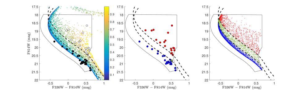
Figure 5.— (Left) CMDs of BSSs combined with our synthetic stellar populations. The filled and open circles represent the blue- and red-branch BSSs, respectively. The mass ratios of our synthetic stars (binaries) are indicated by the color scale. The black dashed curves were adopted to roughly define the gap region between the two branches of BSSs. (Middle) CMDs of BSSs located in the blue branch (blue circles), the red branch (red circles), and the gap (green circle). (Right) As the middle panel, but for the synthetic stars.

3.2. Radial BSS Distribution

If we focus on the region characterized by stellar cluster membership probabilities greater than 50% ($r<16.65$ pc), the numbers of BSSs associated with the red and blue branches are 12 and 15, respectively. (Note that this relates to the number of BSSs in the entire observed field.) If we further constrain the sample of BSSs to cluster membership probabilities exceeding 90% ($r<5.53$ pc), the bifurcated feature is still significant, and the numbers of red- and blue-branch stars are 11 and 7, respectively. Fig. 6 presents three CMDs for BSSs with cluster membership probabilities $P\geq 90$%, $P\geq 70$%, and $P\geq 50$%.

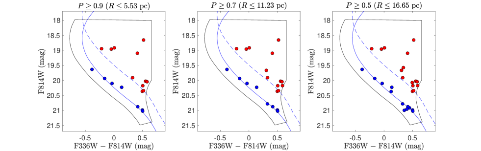
Figure 6.— CMDs of BSSs with different cluster membership probabilities. From left to right, $P\geq 90$%, 70%, and 50%.

In the spatial distributions of the blue- and red-branch BSSs (Fig.7), the red-branch BSSs are likely more centrally concentrated than the blue-branch counterparts. Although the majority of blue-branch stars are located inside the radius characterized by $P\geq 50$% (12/22), a significant fraction of blue-branch stars (10/22) is located beyond the cluster-dominated region. As a comparison, more than 13 of 18 red-branch stars are located inside the $P=50\%$ radius, only 5 of them are located beyond this radius. However, because the number of our BSSs is very small, it is hard to conclude that the red-branch stars are obviously more segregated than blue-branch stars. Our statistical test report that the chance for these two branch stars were drawn from the same parent spatial distribution is 5.35%. That means the significance for their difference in central concentration is 94.65%, corresponding to a 1–2$\sigma$ level significance.

It is possible that most of these latter stars (for both the red- and the blue-branch BSSs) are actually field stars. However, because all observed BSS stars are distributed into two distinct sequences (see Fig. 1), it would be puzzling if field stars of different ages and metallicities would form a clearly bifurcated pattern in the CMD. Another explanation is that most of these stars are genuine BSSs formed in the cluster environment, while the sample stars at larger radii were formed in the core and subsequently ejected to the outer regions by the recoil of stellar interactions (Sigurdsson et al., 1994). These stars, simply based on their spatial distribution, looks like field stars, but are actually cluster members. Alternatively, they may be BSSs that are not yet fully segregated (Ferraro et al., 2012). Since we lack kinematic information for these objects (such as proper motions or radial velocities), we cannot draw any definite conclusions as regards the origin of these BSSs.

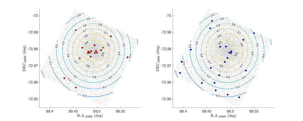
Figure 7.— Spatial distributions of (left) the red- and (right) blue-branch BSSs. Radii characterized by different cluster membership probabilities are indicated.

We explored the radial behavior of these BSSs relative to the bulk population of giant stars (RGB, RC, and AGB stars). We first took both the red- and blue-branch BSSs as our whole sample. We divided the selected sample of BSSs and giant stars into eleven radial bins with intervals of 2.67 pc (i.e., equal to the cluster’s core radius). For each radius, we calculated the number ratio of the BSSs and the giant stars, corrected for stellar incompleteness. Again, stellar completeness was estimated by exploring the difference between the output and the input artificial stellar samples, as shown in the right-hand panels of Fig. 2. The radial profile of the number fraction of the BSSs and the giant stars of NGC 2173 is presented in Fig. 8.

As shown in Fig. 8, the BSS number-fraction profile is noisy in the outer regions ($r>17$ pc), because field stars may be dominant in this region (i.e., $P<50$%). The BSS number-fraction profile in this region may not provide us with any useful information. Instead, we explored their number-fraction profile in the cluster-dominated region ($P<50$%, $r\leq 16.65$ pc). We found that the BSSs’ number-fraction profile is much smoother, exhibiting a seemly bimodal distribution as a function of radius. The minimum number fraction is located between three and four core radii (8.01–10.68 pc). However, we searched for evidence of a bimodal spatial distribution of the entire BSS sample (e.g., Ferraro et al., 2012), and did not find one at 2$\sigma$ level of significance.

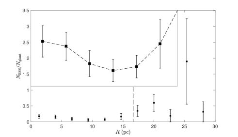
Figure 8.— BSS-fraction profile (normalized to the number of giant stars), corrected for stellar incompleteness. The black dashed line indicates the radius where $P=50$%. The number-fraction profile within this radius is shown in the inset.

We want to emphasize that in this work we do not find a proper way to precisely estimate the effect of field contamination. Because we lack the information of kinetics for our BSSs (such as their radial velocities or proper motions). Because of the large distance to NGC 2173, the kinematics of our BSSs can be only achieved using next-generation telescopes. Readers should be cautious when reach any conclusions based on their radial distributions.

4. Discussion

We first discuss the possible origin of the BSSs in NGC 2173. As shown in Figs 1 and 6, all observed red-branch BSSs are located above the equal-mass binary locus, while the blue sequence resembles the cluster’s ZAMS. As already pointed out, adopting a continuous mass-ratio distribution for a sample of binary systems will unlikely produce such a bifurcated pattern. Low-mass-ratio binaries should have filled the gap between the two BSS branches (for example, see Duquennoy & Mayor, 1991; Milone et al., 2012; Li et al., 2013). In addition, as shown in Fig. 1, NGC 2173 does not show any bifurcated feature in the MS region, further supporting the suggestion that MS–MS binaries are not responsible for the observed bifurcated BSS pattern.

For these reasons, we suggest that this pattern has nothing to do with the ‘single-star versus MS–MS binary relation’ as commonly found for cluster MSs. As shown in Fig. 5, the large dispersion and the position of these red-branch BSSs would imply that they are likely all high mass-ratio binaries. If their companions belong to the old stellar population, they should be more evolved than ZAMS stars, e.g., expanding MSTO stars, subgiant stars, or faint red-giant stars (bright red-giant stars will dominate the total flux of such a binary system and render its photometric locus closer to the RGB rather than the BSS region). This seems to make sense, because a binary system containing an evolved component is more likely to be involved in a mass-transfer process between its member stars, thus producing a rejuvenated BSS. If confirmed, this may imply that a large fraction of these red-branch BSSs are W Ursa Majoris-like objects, similar to the results of Ferraro et al. (2009) for the bifurcated BSSs in the GC M30.

However, although bifurcated BSS populations have also been observed in three old Galactic GCs, where the blue sequences were attributed to core-collapse-driven collisions (Ferraro et al., 2009; Dalessandro et al., 2013; Simunovic et al., 2014), it is unlikely that these blue-sequence BSSs result from direct stellar collisions. Using the equation introduced by Davies et al. (2004), the number of expected collisional BSSs that would be produced in a stellar system over the last 1 Gyr is,

$$N_{\rm col}=0.03225\frac{f^{2}_{\rm mms}N_{\rm c}n_{\rm c,5}r_{\rm col}m_{\rm BSS}}{V_{\rm rel}},$$ (4)

where $f_{\rm mms}$ is the fraction of massive MS stars in the region of interest. Here, ‘massive’ is defined as a mass that is sufficient to form a BSS when two MS stars collide : $f_{\rm mms}=0.25$ is commonly adopted (Davies et al., 2004), and $N_{\rm c}=1.14\times 10^{4}$ is the number of stars contained in the core region. This latter number was evaluated as follows. We calculated the number of stars with masses between $\sim 1.1M_{\odot}$ and $\sim 1.5M_{\odot}$ (corrected for stellar incompleteness). We assumed that these stars follow a Kroupa mass function (Kroupa, 2001) and then evaluated the total number of stars by extrapolating this mass function down to $0.08M_{\odot}$. $n_{c,5}$ is the core density of stars in units of $10^{5}$ pc^-3, which is the ratio of the number of stars contained in the core region and the core volume, yielding $n_{c,5}\sim 0.0014$. $r_{\rm col}$ is the minimum separation of two colliding stars in units of the solar radius, $R_{\odot}$. The average mass of BSSs is $m_{\rm BSS}\sim 2M_{\odot}$. A MS star with this mass would have a radius of $r\sim 1.5R_{\odot}$ (Demircan & Kahraman, 1991). We simply adopted $3R_{\odot}$ for $r_{\rm col}$ (about twice the stellar radius). $V_{\rm rel}$ is the relative incoming velocity of binaries at infinity, which can be written as,

$$V_{\rm rel}=\sqrt{2}\sigma=\sqrt{\frac{4GM_{\rm c}}{r_{\rm c}}},$$ (5)

where $\sigma$ is the stellar velocity dispersion in the core region. $M_{\rm c}$ is the stellar mass of the cluster core, for which we derived $M_{\rm c}\sim 3700$ $M_{\odot}$. The resulting central stellar velocity dispersion for NGC 2173 is $\sigma\sim 3.5$ km s^-1. Our derived stellar velocity dispersion for NGC 2173 is almost twice that found by McLaughlin & van der Marel (2005). This is most likely because we have overestimated the number of stars in the cluster’s core region; numerous low-mass stars must have evaporated from the cluster core owing to dynamical mass segregation (e.g., de Grijs et al., 2002).

We finally obtained $N_{\rm col}=0.04$ for NGC 2173. This means that only $\sim 0.01$ collisional BSSs are expected to have formed over the past 250 Myr and were detected by us in their MS phase. We realize that some higher-order stellar interactions, such as binary–single-star and binary–binary interactions, may increase the production rate of collisional BSSs. The realistic number of collisional BSSs produced should still be of the same order, however (Davies et al., 2004). The negligibly small number of expected collisional BSSs formed within the last 250 Myr excludes stellar collisions as a possible origin of the observed tight blue-branch BSS stars. Indeed, as shown in Fig. 4, NGC 2173 exhibits a very extended core region. This is in contrast to the structures of GCs exhibiting distinct BSS sequences, which often show cusps in their central regions, apparently driven by core-collapse events (Ferraro et al., 2009; Dalessandro et al., 2013).

Another possible explanation is that NGC 2173 may already have experienced a core-collapse event and has remained in the post-core-collapse bounce state, similar to that found for the old GC NGC 1261 (Simunovic et al., 2014). However, it is unclear if a core-collapse event could occur in such a young cluster. Trenti et al. (2010) calculated that the minimum core-collapse timescale for a star cluster is about 5.8 times its half-mass relaxation timescale (their Fig. 7). Based on McLaughlin & van der Marel (2005), the half-mass relaxation timescale pertaining to NGC 2173 is at least 2.09 Gyr. Therefore, there is no obvious evidence that supports the notion that NGC 2173 may have experienced a core-collapse event.

Our statistical analysis shows that the observed blue-branch BSSs are tightly associated with the ZAMS. This fact may indicate that most blue-branch BSSs actually originate from single stars. However, this immediately leads to another conundrum. Since only stellar collisions or binary mergers can result in a BSS that is not presently a member of a binary system, the only viable explanation of these blue-branch BSSs is that they are binary merger products. However, we have already excluded stellar collisions as an efficient channel to produce these BSSs. If this is correct, the tight blue sequences may indicate that most binaries merged over very short time intervals. Why would so many binary merger events happen over a short period? The answer to this question remains to be resolved. Future analysis focusing on details of the cluster’s dynamics, such as its mass segregation, binary hardening, and mass exchange, may be able to shed light on this outstanding problem.

5. Summary

In this article, we report the detection of a bifurcated BSS pattern in the CMD of NGC 2173. This is the first detection of such a feature in a star cluster that is much younger than the typical GC age. Our main results and conclusions can be summarized as follows:

• The overall distribution of BSSs in NGC 2173 is divided into two sequences with a significance of equal to or greater than 3$\sigma$ level. The blue-sequence BSSs are tightly associated with a single-age isochrone with an age of $\sim$250 Myr. The red-sequence BSSs exhibit a lower boundary that is close to the equal-mass MS–MS binary locus for an age of $\sim$250 Myr. In the CMD, the red-branch BSSs are more dispersed than blue-branch BSSs

• The red-branch BSSs are more centrally concentrated than blue-branch BSSs with a significance level of close to $\sim$2$\sigma$.

• Stellar collisions are unlikely responsible for these BSSs because of the cluster’s low stellar central number density. In addition, the number-density profile of NGC 2173 exhibits an extended core with a size of $\sim$2.67 pc, indicating that NGC 2173 has not experienced any core-collapse event.

• We suggest that only binary evolution is able to explain the presence of these BSSs. However, why binary evolution would result in a BSS distribution composed of two distinct sequences in the cluster’s CMD remains unclear.

References

- Andronov et al. (2006) Andronov, N., Pinsonneault, M. H., & Terndrup, D. M. 2006, ApJ, 646, 1160
- Baldwin et al. (2016) Baldwin, A. T., Watkins, L. L., van der Marel, R. P., et al. 2016, ApJ, 827, 12
- Baumgardt et al. (2013) Baumgardt, H., Parmentier, G., Anders, P., & Grebel, E. K. 2013, MNRAS, 430, 676
- Boffin et al. (2015) Boffin, H. M. J., Carraro, G., & Beccari, G. 2015, Ecology of Blue Straggler Stars,
- Bressan et al. (2012) Bressan, A., Marigo, P., Girardi, L., et al. 2012, MNRAS, 427, 127
- Cohn (1980) Cohn, H. 1980, ApJ, 242, 765
- Dalessandro et al. (2013) Dalessandro, E., Ferraro, F. R., Massari, D., et al. 2013, ApJ, 778, 135
- Davies et al. (2004) Davies, M. B., Piotto, G., & de Angeli, F. 2004, MNRAS, 349, 129
- de Grijs et al. (2002) de Grijs, R., Gilmore, G. F., Johnson, R. A., & Mackey, A. D. 2002, MNRAS, 331, 245
- Demircan & Kahraman (1991) Demircan, O., & Kahraman, G. 1991, Ap&SS, 181, 313
- Duquennoy & Mayor (1991) Duquennoy, A., & Mayor, M. 1991, A&A, 248, 485
- Ferraro et al. (2003) Ferraro, F. R., Sills, A., Rood, R. T., Paltrinieri, B., & Buonanno, R. 2003, ApJ, 588, 464
- Ferraro et al. (2009) Ferraro, F. R., Beccari, G., Dalessandro, E., et al. 2009, Nature, 462, 1028
- Ferraro et al. (2012) Ferraro, F. R., Lanzoni, B., Dalessandro, E., et al. 2012, Nature, 492, 393
- Fregeau et al. (2004) Fregeau, J. M., Cheung, P., Portegies Zwart, S. F., & Rasio, F. A. 2004, MNRAS, 352, 1
- Grocholski et al. (2007) Grocholski, A. J., Sarajedini, A., Olsen, K. A. G., Tiede, G. P., & Mancone, C. L. 2007, AJ, 134, 680
- Hills & Day (1976) Hills, J. G., & Day, C. A. 1976, Astrophys. Lett., 17, 87
- King (1962) King, I. 1962, AJ, 67, 471
- Knigge et al. (2009) Knigge, C., Leigh, N., & Sills, A. 2009, Nature, 457, 288
- Kroupa (2001) Kroupa, P. 2001, MNRAS, 322, 231
- Li et al. (2013) Li, C., de Grijs, R., Deng, L., & Liu, X. 2013, ApJ, 770, L7
- Li et al. (2013) Li, C., de Grijs, R., & Deng, L. 2013, MNRAS, 436, 1497
- Lynden-Bell & Eggleton (1980) Lynden-Bell, D., & Eggleton, P. P. 1980, MNRAS, 191, 483
- Mathieu & Geller (2009) Mathieu, R. D., & Geller, A. M. 2009, Nature, 462, 1032
- McCrea (1964) McCrea, W. H. 1964, MNRAS, 128, 147
- McLaughlin & van der Marel (2005) McLaughlin, D. E., & van der Marel, R. P. 2005, ApJS, 161, 304
- Meylan (1987) Meylan, G. 1987, A&A, 184, 144
- Milone et al. (2009) Milone, A. P., Bedin, L. R., Piotto, G., & Anderson, J. 2009, A&A, 497, 755
- Milone et al. (2012) Milone, A. P., Piotto, G., Bedin, L. R., et al. 2012, A&A, 540, A16
- Perets & Fabrycky (2009) Perets, H. B., & Fabrycky, D. C. 2009, ApJ, 697, 1048
- Sandage (1953) Sandage, A. R. 1953, AJ, 58, 61
- Sigurdsson et al. (1994) Sigurdsson, S., Davies, M. B., & Bolte, M. 1994, ApJ, 431, L115
- Simunovic et al. (2014) Simunovic, M., Puzia, T. H., & Sills, A. 2014, ApJ, 795, L10
- Stryker (1993) Stryker, L. L. 1993, PASP, 105, 1081
- Trenti et al. (2010) Trenti, M., Vesperini, E., & Pasquato, M. 2010, ApJ, 708, 1598
- Xin & Deng (2005) Xin, Y., & Deng, L. 2005, ApJ, 619, 824
- Zinn & Searle (1976) Zinn, R., & Searle, L. 1976, ApJ, 209, 734