Quantum Phase Transitions in Proximitized Josephson Junctions

Abstract

We study fermion-parity-changing quantum phase transitions (QPTs) in platform Josephson junctions. These QPTs, associated with zero-energy bound states, are rather widely observed experimentally. They emerge from numerical calculations frequently without detailed microscopic insight. Importantly, they may incorrectly lend support to claims for the observations of Majorana zero modes. In this paper we present a fully consistent solution of the Bogoliubov-de Gennes equations for a multi-component Josephson junction. This provides insights into the origin of the QPTs. It also makes it possible to assess the standard self energy approximations which are widely used to understand proximity coupling in topological systems. The junctions we consider are complex and chosen to mirror experiments. Our full proximity calculations associate the mechanism behind the QPT as deriving from a spatially extended, proximity-induced magnetic “defect”. This defect arises because of the insulating region which effects a local reorganization of the bulk magnetization in the proximitized superconductor. Our results suggest more generally that QPTs in Josephson junctions generally do not require the existence of spin-orbit coupling and should not be confused with, nor are they indicators of, Majorana physics.

I Introduction

Josephson junction geometries, particularly in the presence of magnetic fields, are becoming of greater interest in the search for and confirmation of topological superconductors. Often present in these spinful Josephson junctions are fermion-parity switches. A fermion-parity switch is a quantum phase transition (QPT) where the superconducting condensate can lower its ground state energy by incorporating an unpaired electron and changing the number of electrons in the ground state from even to odd. This results in zero-energy bound states and energy level crossings which are protected (due to fermion parity) and are, thus, not lifted by a superconducting gap. The QPTs of interest here are claimed by some Sau and Demler (2013); Cayao et al. (2015); Lee et al. (2017) to be important indicators of topological phases. Others Peng et al. (2015); Chang et al. (2013) argue that they may be more “accidental” and they, rather, make it difficult to distinguish the interesting Majorana quasi-particles from conventional fermionic subgap states.

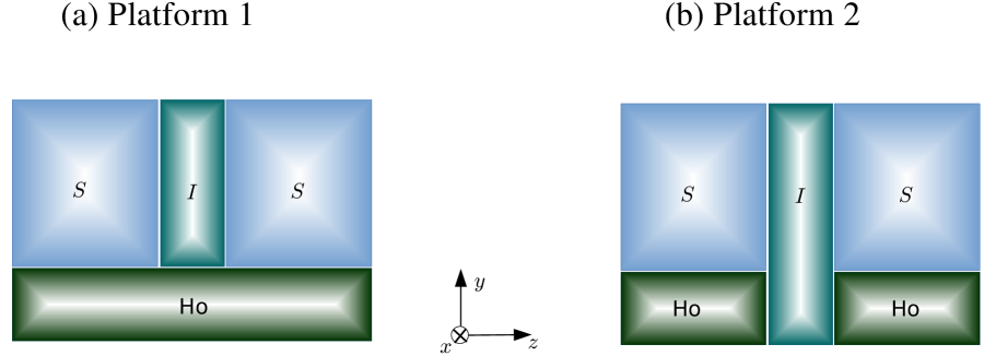
Figure 1: Schematic illustration of proximitized Josephson junctions. Two types of platforms are considered in this work. Platform 1 is a typical Josephson junction with an insulating barrier placed on top of a conical ferromagnet (Ho) substrate with effective spin-orbit and Zeeman coupling. In platform 2, two conical-ferromagnet/superconductor bilayers are separated by an insulating barrier. Both platforms are assumed to be finite along the $y$ and $z$ directions, but infinite along the $x$-direction.

Because it is not clear the extent to which these QPTs relate to topological superconductivity, and to clarify their origin more generally, in the present paper we investigate their behavior in Josephson junctions. We study a “proximitized” Josephson junction which includes two host superconductors which induce pairing in a substrate medium. The latter contains both Zeeman and spin-orbit coupling (SOC), as necessary for topological phases. We solve the the full set of BdG equations in this multi-component system. This makes it possible to assess the standard self energy approximations Sau et al. (2010); Stanescu et al. (2010); Stanescu and Das Sarma (2017); Stanescu et al. (2011); Hell et al. (2017) which are widely used to implement proximity coupling in topological materials.

Our fully self consistent treatment allows us to compute the induced magnetization $\bf{m}(\bf{r})$, in the junction. These calculations indicate that the non-topological zero energy bound states are confined to regions where $\bf{m}(\bf{r})$, is most inhomogeneous. This suggests a scenario for the bound state origin involving a proximity-induced “magnetic” defect. Although we build on some of the formal similarities, it is important to contrast this with an inserted magnetic impurity in a superconducting host Yu (1965); Shiba (1968); Sakurai (1970). Here we associate the “magnetic defect” with the insulating region which effects a local reorganization of the magnetization in the proximitized medium. Central to obtaining quantum phase transitions in this picture is the presence of Zeeman fields in the junctions.

We consider two types of geometries as shown in Fig. 1. The first platform contains a holmium (Ho) substrate in the $xz$ plane on top of which are placed two superconductors separated by an insulator I. Although we believe our results to be quite general, for definiteness we take the proximitized superconductor to be a conical magnet (Ho) which the spintronics community has established Linder and Robinson (2015) exhibits well-controlled and well-characterized proximity coupling. Importantly, in Ho the Zeeman and SOC are intrinsically present. The conical magnetism implies that the SOC is effectively one dimensional (1D), as distinguished from Rashba SOC. And interestingly it is possible to control the 1D SOC with a very benign or non-intrusive “knob” Bernardo et al. (2015), through the unwinding of the conical order.

For the second platform, we consider two Ho-Superconductor (Ho-S) bilayers in contact with an intermediate insulating layer. Both platforms are assumed to have finite thicknesses in the $y$ and $z$ directions as shown in Fig. 1 and are taken to be infinite along $x$. We stress that, in both platforms, two conventional superconductors are used to induce superconducting order in Ho which has no intrinsic pairing. This proximity-induced superconductivity is characterized by solving the Bogoliubov-de Gennes (BdG) equations with the incorporation of full self-consistency. Introducing two different junction configurations allows us to further contrast the behavior of trivial versus topological zero energy bound states. In both platforms and in topological phases one can access bound states which are associated with Majorana particles. We find that platform 1 also hosts trivial zero energy bound states which we associate with magnetization inhomogeneities. Platform 2, by contrast, does not contain these trivial crossings; rather it only hosts true (albeit, hybridized) Majorana states.

Our QPTs should also be relevant to the broader, and topical issue of zero bias conductance peaks. Here, too, there are reports of QPT, often not associated with topological phases Liu et al. (2012); Bagrets and Altland (2012); Pikulin et al. (2012). While the literature on topological Josephson junctions has focused on proximity-induced superconductivity primarily in nanowires, in order to emphasize QPTs and level crossings, the junctions we contemplate extend indefinitely into the $x$ dimension; this conveniently introduces a variable $k_{x}$ thereby providing continuous tuneability and, importantly, wider access to zero-energy bound states, fermion-parity switches and level crossings.

Notably, we find that all this interesting physics arises via proximity-induced superconductivity. While the nature and location of the zero-energy bound states were not obvious a priori, one might have erroneously anticipated that they relate to states within the insulator. However, we find them here to be almost exclusively localized in the proximitized superconductors (in this case, Ho).

I.1 Background Literature

Relevant to the work in this paper is our earlier study Wu et al. (2017) of a two component Ho-S proximity system. There we have shown that the end result is a heterostructural nodal topological superconductor. By studying the fully self consistent BdG equations in finite size systems, we have demonstrated how excitation gaps and general features of topological energy dispersion along with Majorana zero modes are found to be present.

Turning now to Josephson junctions, fermion parity shifts in QPTs and associated energy level crossings have appeared most commonly in the literature in two related (non-topological) contexts associated with localized magnetic impurities (such as the Shiba state) as well as in tunnel junctions involving quantum dots (QD) Kiršanskas et al. (2015); Peng et al. (2015); Chang et al. (2013); Lee et al. (2014a, 2017); Deacon et al. (2010) with strong Coulomb correlation. In the latter context the quantum dots are thought to contain trapped spin 1/2 single electrons which play a similar role as magnetic impurities. They, thus, can host two distinct ground states Yu (1965); Shiba (1968); Sakurai (1970), which in turn can lead to fermion parity shifts.

In a somewhat different vein, based on the physics of Shiba states, Sau and Demler Sau and Demler (2013) suggest that non-magnetic impurities may be used as a probe of topological superconductivity Alicea (2012); Beenakker (2013); Elliott and Franz (2015). They argue that in the topological phase, a non-magnetic impurity will lead to distinctive pairbreaking due to the associated $p$-wave symmetry. Yazdani and co-workers Li et al. (2016, 2014) have inverted this situation in a sense by using magnetic impurities to bind fermions into a 1D Kitaev-chain which can then play the role of a nanowire with topological superconducting order.

Parity switches and related zero-energy bound states, of interest in the present paper, have also led to a lively debate about recent experiments Mourik et al. (2012); Deng et al. (2016) which claim evidence for Majorana fermions. These have mainly focused on zero bias conductance peaks. Liu and co-workers have recently Liu et al. (2017) studied how Andreev bound states associated with quantum dots may produce near-zero-energy midgap states as the Zeeman splitting and/or chemical potential are tuned. They find the behavior as a function of magnetic field and chemical potential is sufficiently complex so that one cannot arrive at simple governing equations. These zero-energy Andreev bound states (ABSs) mostly appear in the nontopological regime; here the quantum dot was assumed to have no Coulomb blockade behavior.

In the trivial phase, others Liu et al. (2012); Bagrets and Altland (2012); Pikulin et al. (2012) have demonstrated how near-zero-energy states may arise in a spin-orbit coupled nanowire (in the presence of a magnetic field) and associated these with disorder effects or details in the wire’s end or even temperature. Because of these and related papers, it is natural for there to be concern that zero-energy bound states related to parity switches can give rise Peng et al. (2015) to features which could be confused with topological phases; thus, they need to be well understood before they can be safely disregarded.

I.2 Proximity Effects

We stress that most of the current thinking about topological superconductivity is based on the proximity effect. A fully complete and detailed treatment of this proximitization is complicated Klapwijk (2004). Moreover, for the case of Josephson junctions we know of no prior, fully precise calculations in the topological literature. Proximity effects are conventionally handled Sau et al. (2010); Stanescu et al. (2010); Stanescu and Das Sarma (2017); Stanescu et al. (2011); Hell et al. (2017) through a simplification, by integrating out the (host) superconducting degrees of freedom. This introduces an effective self energy term in the proximitized medium. In this way a pairing gap is assumed to be present, but it is generally taken to be piece-wise constant (or zero) in different regions of the heterostructure.

How good are these approximations and how accurately do they represent the more exact physics? These are questions we address in this paper in the context of Josephson junctions. Here we use an alternate methodology Halterman and Valls (2001) developed for ferromagnet-superconductor junctions in spintronics. This involves a complete solution of the BdG equations for a given heterostructure. As is physical, the pairing attraction is assumed present only in the host superconductors. Proximitization introduces a non-vanishing value for the so-called pair amplitude $F({\bf r})=\langle\psi_{\downarrow}({\bf r})\psi_{\uparrow}({\bf r})\rangle$. Importantly, these induced pairing correlations which appear in a non-superconducting system can be sufficiently strong so as to produce a Meissner effect Klapwijk (2004). Unlike in an intrinsic superconductor, however, the phase coherence of these pairing correlations is maintained only over a restricted length scale  Halterman and Valls (2002).

To understand the proximity findings in the present paper more deeply, we present a comparison of the full BdG solution with the widely used self-energy scheme Sticlet et al. (2017); Stanescu et al. (2010); Stanescu and Das Sarma (2017); Hell et al. (2017). This leads to a 3 component SIS structure (with infinite extent in the $x$ direction). What emerges from this comparison of the full versus the approximate treatment of proximity effects is that for both platforms there are broad-based similarities. For the first the QPT we find are associated with the trivial, while for the second they appear in the topological phase. We note that the energy dispersions in the two theoretical approaches appear rather differently and it is often difficult to access the same parameter regime, particularly in the second platform. This is discussed in more detail in Section IV.

I.3 Zero-Energy crossing as a zero dimensional topological phase transition

It is important to understand the zero-energy crossings (ZECs) in these SIS junctions in more depth. It is known that such crossings in the energy spectrum are signatures of a (zero dimensional) topological phase transition involving a change in fermion parity.

As in a topological superconductor, a fermion-parity changing QPT can be understood through a change in the Pfaffian of the BdG Hamiltonian. In particular, near a crossing point $k_{\mathrm{c}}$ we may project the Hamiltonian onto the subspace spanned by the corresponding two crossed states denoted $|\pm\rangle$ so that the resulting two-band effective Hamiltonian is given by

$$H^{mn}_{\mathrm{eff}}=\langle m|\nabla_{k_{x}}H|n\rangle\delta k_{x},$$ (1.1)

where $m,n=\pm$. By diagonalizing the effective Hamiltonian, we obtain

$$H_{\mathrm{eff}}=A\delta k_{x}\sigma_{z},$$ (1.2)

where $\sigma_{x,y,z}$ are the Pauli matrices acting in the $|\pm\rangle$ subspace. By performing a basis rotation, we can write Eq. (1.2) into its skew-symmetric form:

$$H_{\mathrm{eff}}=A\delta k_{x}\sigma_{y}.$$ (1.3)

The Pfaffian of this skew-symmetric Hamiltonian is simply sgn($A$). Since the sign of $H_{\mathrm{eff}}$ changes at the crossing point (unless $A=0$), its Pfaffian changes. Moreover, since $H_{\mathrm{eff}}$ is a $2\times 2$ block in the full Hamiltonian, the Pfaffian of the full Hamiltonian changes as well. Hence, this is a topological phase transition between two different “phases” in class BDI.

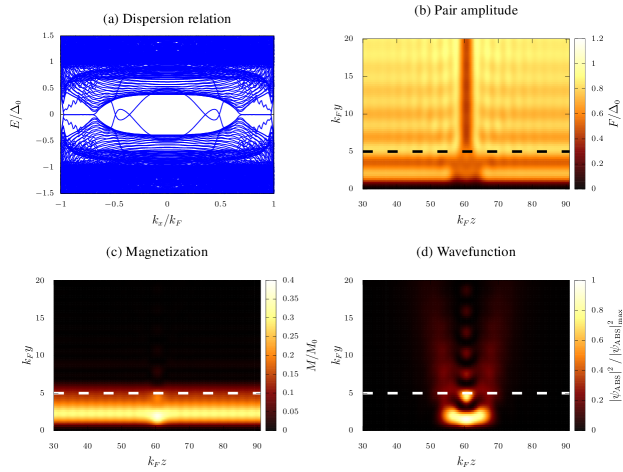
Figure 2: Results from the first Josephson platform for (a) the energy dispersion versus $k_{x}$, (b) the pair amplitude, (c) the magnetization and, (d) the wavefunction at a crossing point. The phase difference between the two superconducting leads is set to be zero. In panel (a) the flat bands on two wings of this plot are associated with Majorana edge modes whereas the linear crossings in the central region are associated with the localized “impurity” Andreev bound states, caused by the insulating defect. In panel (c) there is a local maximum in the magnetization in the Ho region just below the insulator. We normalize the magnetization $M$ by $M_{0}\equiv\mu_{B}(n_{\uparrow}-n_{\downarrow})/(n_{\uparrow}+n_{\downarrow})$, where $n_{\sigma}$ is the spin density. The bottom right panel shows a typical localized wavefunction associated with a crossing state at $k_{x}=0.36k_{F}$; this is in the same region as the magnetization inhomogeneity. The boundary between the Josephson junction and the substrate is represented by dashed lines. We choose the thickness of the two superconductors along the $y$-axis to be $d_{S}=75k_{F}^{-1}$ and the length of them to be $l_{S}=60k_{F}^{-1}$ along the $z$-axis. The superconducting coherence length is $\xi=2/(\pi\Delta_{0})=10k_{F}^{-1}$. The chemical potential in the insulator is chosen to be $\mu_{I}=-2E_{F}$ and the exchange interaction in Ho is $0.2E_{F}$. The insulating region has a width $\ell_{I}=0.1\xi$ (from $z=60k_{F}^{-1}$ to $z=61k_{F}^{-1}$). The thickness of the Ho substrate is $d_{\rm Ho}=0.5\xi$ (from $y=0$ to $y=5k_{F}^{-1}$).

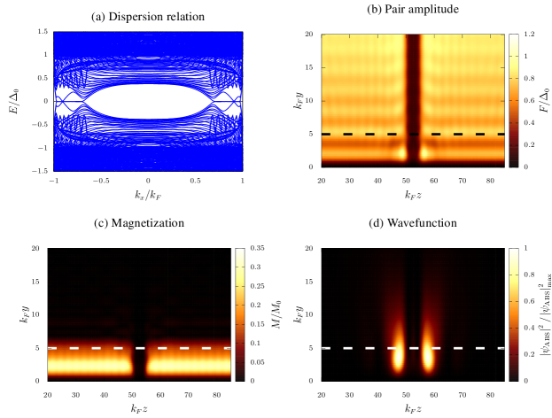
Figure 3: Results for the second Josephson platform in which the zero energy crossing corresponds to two Majorana states in the middle of the Junction. (a) Energy dispersion versus $k_{x}$, (b) The pair amplitude, (c) magnetization and (d) the wavefunction at a crossing point. The phase difference between two superconducting leads is set to be zero. In panel (a) the flat bands on two wings of this plot are associated with Majorana edge modes at the ends of Holmium away from the junction. whereas the linear crossings are associated with two Majorana modes at the Ho/I interfaces. The self-consistent pair amplitudes, shown in panel (b) are suppressed in the insulating region. The magnetization (c) turns on abruptly just beyond the insulating region. Panel (d) shows that the localized wavefunction amplitude ($k_{x}=0.90k_{F}$) becomes large just where the magnetic inhomogeneity appears. The boundary between the S layers and the Ho layers is represented by dashed lines. We choose the thickness of the two superconductors along the $y$-axis to be $d_{S}=75k_{F}^{-1}=7.5\xi$. where $\xi$ is the superconducting coherence length. The thickness of the Holmium is $d_{\rm Ho}=5k_{F}^{-1}=0.5\xi$. The length of the Holmium/superconductor bilayers along the $z$-axis is taken to be $\ell_{S}=\ell_{\mathrm{Ho}}=40k_{F}^{-1}=4\xi$. The chemical potential of the superconductor and Holmium are taken to be $\mu_{S}=\mu_{\mathrm{Ho}}=E_{F}$. The chemical potential in the insulator, which separates two bilayers, is chosen to be $\mu_{I}=-2E_{F}$ and its width is $\ell_{I}=5k_{F}^{-1}$. The exchange field in the conical ferromagnets is $0.2E_{F}$.

I.4 Self Consistency in Bogoliubov-de Gennes Theory

In this overview section we outline the general structure of self-consistent BdG schemes. More specific details of this approach are given in the following section. Self-consistency involves solving for the pair amplitude $F({\bf r})\equiv\langle\psi_{\uparrow}(\bf{r})\psi_{\downarrow}({\bf r})\rangle$ at a microscopic level in terms of the attractive interaction. This is to be contrasted with the more standard BdG approach in the recent literature (on topological superconductivity) which is to solve the same equations for the wavefunctions and energies, but not include the feedback of these wavefunctions into the determination of the gap.

We stress that imposing a self-consistent gap equation is fundamental to BCS theory and its extensions to non-uniform situations such as in Gor’kov theory or the equivalent BdG approach. Proximitized superconductors necessarily involve spatially dependent gap functions; fixing the gap value to be constant in a certain region of the sample may make the calculations easier, but they may miss essential physics which is particularly relevant at interfaces and boundaries. Here we use these (sometimes abrupt) spatial variations in the pair amplitude and in derived quantities such as the magnetization to establish correlations and thereby provide insight into quantum phase transitions.

Our system can be described by the following mean-field Hamiltonian

$$\mathcal{H} =\int d^{3}\mathbf{r}\psi_{\sigma}^{\dagger}(\mathbf{r})\left(H_{0}+H_{\rm Zeeman}\right)_{\sigma\sigma^{\prime}}\psi_{\sigma^{\prime}}(\mathbf{r})$$

$$+\left[\Delta(\mathbf{r})\psi_{\uparrow}^{\dagger}(\mathbf{r})\psi_{\downarrow}^{\dagger}(\mathbf{r})+\textrm{H.c.}\right],$$ (1.4)

where $\psi_{\sigma}^{\dagger}(\mathbf{r})$ ($\psi_{\sigma}(\mathbf{r})$) with spin $\sigma=\uparrow,\downarrow$ are fermionic creation (annihilation) operators and $H_{0}$ is the single particle contribution. An attractive pairing interaction is only present in the superconductors. Here $H_{\rm Zeeman}={\bf h}\cdot{\bm{\sigma}}$ is the Zeeman term in the full Hamiltonian, Eq. (1.4), where ${\bm{\sigma}}=\left(\sigma_{x},\sigma_{y},\sigma_{z}\right)$ are Pauli matrices and ${\bf h}$ is the exchange interaction associated with a conical magnet which is given by

$${\bf h}=h_{0}\left\{\cos\alpha\hat{z}+\sin\alpha\left[\sin\left(\frac{\beta z}{a}\right)\hat{x}+\cos\left(\frac{\beta z}{a}\right)\hat{y}\right]\right\},$$ (1.5)

Here $\beta$ is the periodicity of the helix and $a$ is the lattice constant along the $c$ axis of Holmium. As in the literature Chiodi et al. (2013); Halász et al. (2009), the opening angle $\alpha=\pi/2$. From our previous analysis Wu et al. (2017), this puts our model Hamiltonian in the BDI class. The spiral magnetic order introduces a combination of one-dimensional spin-orbit coupling (SOC) and Zeeman field Nadj-Perge et al. (2013); Martin and Morpurgo (2012). This can be shown by applying a gauge transformation $\psi_{\uparrow}\rightarrow e^{-i\beta z/2a}\psi_{\uparrow}$ and $\psi_{\downarrow}\rightarrow e^{i\beta z/2a}\psi_{\downarrow}$ which transforms the single-particle Hamiltonian into

$$H^{\prime}_{0}+H^{\prime}_{\mathrm{Zeeman}}=H_{0}-v_{so}\sigma_{z}i\partial_{z}+mv^{2}_{\mathrm{so}}/2+\mathbf{h}^{\prime}\cdot\bm{\sigma},$$ (1.6)

where the effective Zeeman strength is $\mathbf{h}^{\prime}=h_{0}(\sin\alpha\hat{\bf{x}}+\cos\alpha\hat{\bf{z}})$ and the spin-orbit-coupling strength is $v_{\mathrm{so}}=\frac{\beta}{2ma}$. In this way, the magnetic spiral period $\lambda=2\pi a/\beta$ sets the strength of the spin-orbit coupling $v_{\mathrm{so}}=\pi/(m\lambda)$.

The BdG equation in matrix form is given by,

$$\left(\begin{array}[]{cccc}H_{0}&h_{x}-ih_{y}&0&\Delta\\ h_{x}+ih_{y}&H_{0}&-\Delta&0\\ 0&-\Delta^{\ast}&-H_{0}&-h_{x}+ih_{y}\\ \Delta^{\ast}&0&-h_{x}-ih_{y}&-H_{0}\end{array}\right)\left(\begin{array}[]{c}u_{n\uparrow}\\ u_{n\downarrow}\\ v_{n\uparrow}\\ v_{n\downarrow}\\ \end{array}\right)$$ (1.15)

$$=E_{n}\left(\begin{array}[]{c}u_{n\uparrow}\\ u_{n\downarrow}\\ v_{n\uparrow}\\ v_{n\downarrow}\\ \end{array}\right),$$ (1.20)

where $u_{n\sigma}$ ($v_{n\sigma}$) are quasi-particle (hole) wavefunctions. We have suppressed the position label, $\bf r$, in Eq. (1.20). The Hamiltonian in Eq. (1.20) can be written more compactly in the Nambu basis as

$$\mathcal{H_{\mathrm{BdG}}}=H_{0}\tau_{z}+\mathbf{h}.\bm{\sigma}\tau_{z}+[i\Delta\sigma_{y}\tau_{+}+\mathrm{H.c.}],$$ (1.21)

where $\bm{\sigma}$ and $\bm{\tau}$ are the Pauli matrices acting in the spin and particle-hole subspaces, respectively.

Now the essence of a self-consistent BdG approach is to obtain the superconducting pair potential (or “gap” parameter), $\Delta({\bf r})$, microscopically from the attractive interactions:

$$\Delta({\bf r})\equiv g({\bf r})F({\bf r}),$$ (1.22)

where $g({\bf r})$ is the coupling constant which vanishes outside the superconductor Halterman and Valls (2001) and

$$F({\bf r})=\sum_{\epsilon_{n}<\omega_{D}}\left[u_{n\uparrow}({\bf r})v_{n\downarrow}^{*}({\bf r})-u_{n\downarrow}({\bf r})v_{n\uparrow}^{*}({\bf r})\right]\tanh\left(\frac{\epsilon_{n}}{2T}\right)$$ (1.23)

is the pair amplitude. Note that the Debye frequency $\omega_{D}$ is the energy cutoff and $T$ is the temperature (we set $\omega_{D}=0.1E_{F}$ and $T=0$ in this paper). Important for the present purposes is that in our proximitized superconductors, the pair amplitude is non-zero, even though there is a vanishing order parameter.

Another important physical property which involves $u_{\sigma}$ and $v_{\sigma}$ is the position-dependent magnetization.

$$m_{x}({\bf r})= -\mu_{B}\sum_{n}\left(v_{n\uparrow}({\bf r})v_{n\downarrow}^{\ast}({\bf r})+v_{n\downarrow}({\bf r})v_{n\uparrow}^{\ast}({\bf r})\right),$$ (1.24a)

$$m_{y}({\bf r})= i\mu_{B}\sum_{n}\left(v_{n\uparrow}({\bf r})v_{n\downarrow}^{\ast}({\bf r})-v_{n\downarrow}({\bf r})v_{n\uparrow}^{\ast}({\bf r})\right),$$ (1.24b)

$$m_{z}({\bf r})= -\mu_{B}\sum_{n}\left(|v_{n\uparrow}({\bf r})|^{2}-|v_{n\downarrow}({\bf r})|^{2}\right),$$ (1.24c)

where $\mu_{B}$ is the Bohr magneton. This is a central quantity in the present paper. The spatial dependence of the magnetization $M({\bf r})=\sqrt{m_{x}^{2}+m_{y}^{2}+m_{z}^{2}}$ is associated with a magnetic screening cloud in the superconductor. Of interest is how in a proximitized superconductor, the magnetization can be reorganized (say, by insulating barriers, defects and interfaces) in a way which is readily quantified.

II BdG Approach for proximity calculations

II.1 Numerical procedure

The single particle term in the full Hamiltonian which appears in Eq. (1.4) is

$$H_{0}=-\frac{\nabla^{2}}{2m}-\mu(y,z).$$ (2.1)

This describes free fermions of mass $m$. Throughout the paper we adopt the natural units $\hbar=k_{B}=1$. The insulator is associated with the position-dependent quantity $U_{0}(y,z)$ which reflects a localized shift in the chemical potential. We use a single positive Fermi energy $E_{F}$ for the chemical potentials of the superconducting layers $\mu_{S}$ and the substrate $\mu_{\mathrm{Ho}}$. The chemical potential $\mu_{I}$ for the insulator should be negative. More precisely, the shift of the insulating Fermi level takes the form $U_{0}(y,z)=$

$$E_{F}-\left(E_{F}-\mu_{I}\right)\Theta\left(y-d_{\rm Ho}\right)\Theta\left(z-\ell_{S}\right)\Theta\left(\ell_{S}+\ell_{I}-z\right)$$ (2.2)

in the first platform and

$$E_{F}-\left(E_{F}-\mu_{I}\right)\Theta\left(z-\ell_{S}\right)\Theta\left(\ell_{S}+\ell_{I}-z\right)$$ (2.3)

in the second platform. We define $d_{\mathrm{Ho}}$, $d_{S}$, $\ell_{I}$, and $\ell_{S}$ as respectively the thickness of the Ho substrate (along the $y$-direction), thickness of the superconductor (along the $y$-direction), the length of the insulator (along the $z$-direction), and the length of the superconductor (along the $z$-direction). (For simplicity, we take the two S layers in these platforms to be the same along both $y$- and $z$-direction). The origin of the $y-z$ coordinate system is at the bottom left corner for both junction configurations as shown in Fig. 1.

Because the Hamiltonian is translationally invariant along $x,$ the proposed wavefunction in the $x$ direction is in the form of $e^{ik_{x}x}.$ Therefore,

$$H_{0}=-\frac{1}{2m}\left(\partial_{y}^{2}+\partial_{z}^{2}\right)+\frac{k_{x}^{2}}{2m}-\mu(y,z).$$ (2.4)

The attractive pairing interaction $g$ is also a function of $y$ and $z$ and taken to be a constant associated with a bulk superconductor in the S regions.

We numerically solve the BdG eigenvalue problem following the scheme developed in Refs. Wu et al. (2012, 2017); Halterman and Valls (2001). For definiteness, we set the smallest length scale to be in the order of $k_{F}^{-1}$. We then expand both the matrix elements and the eigenfunctions in terms of a Fourier basis.

For the quasi-particle and quasi-hole wavefunctions, we have

$$\tilde{u}_{n\sigma k_{x}}(y,z) = \frac{2}{\sqrt{d\ell}}\sum_{p,q}u_{n\sigma k_{x}}^{pq}\sin\left(\frac{p\pi y}{d}\right)\sin\left(\frac{q\pi z}{\ell}\right),$$ (2.5a)

$$\tilde{v}_{n\sigma k_{x}}(y,z) = \frac{2}{\sqrt{d\ell}}\sum_{p,q}v_{n\sigma k_{x}}^{pq}\sin\left(\frac{p\pi y}{d}\right)\sin\left(\frac{q\pi z}{\ell}\right).$$ (2.5b)

Note that $\tilde{u}_{n\sigma k_{x}}$ and $\tilde{v}_{n\sigma k_{x}}$ are related to ${u}_{n\sigma}$ and ${v}_{n\sigma}$ by the relations $u_{n\sigma}=e^{ik_{x}x}\tilde{u}_{n\sigma k_{x}}$ and $u_{v\sigma}=e^{ik_{x}x}\tilde{v}_{n\sigma k_{x}}$. General matrix elements are similarly expanded in terms of the same Fourier series. For example, we define the matrix elements of an operator $O$ to be

$$O^{pqp^{\prime}q^{\prime}} \equiv \langle pq|O|p^{\prime}q^{\prime}\rangle$$ (2.6)

$$= \frac{4}{d\ell}\int_{0}^{d}\int_{0}^{\ell}dydz\sin\left(\frac{p\pi y}{d}\right)\sin\left(\frac{q\pi z}{\ell}\right)$$

$$\qquad\times O\sin\left(\frac{p^{\prime}\pi y}{d}\right)\sin\left(\frac{q^{\prime}\pi z}{\ell}\right).$$

All terms in the Hamiltonian can then be expanded in this basis set. We then have successfully transformed a set of differential equations into an algebraic matrix eigenvalue problem. To consider a phase difference $\phi$ between the two superconductors, our initial ansatz for the pair potential is: $\Delta(y,z)=$

$$\Delta_{0}\Theta\left(y-d_{\rm Ho}\right)\left[\Theta\left(\ell_{S}-z\right)+\Theta\left(z-\ell_{S}-\ell_{I}\right)e^{i\phi}\right],$$ (2.7)

for both platforms, where $\Delta_{0}$ is the bulk superconducting pair amplitude. As in our previous work Wu et al. (2017), we look for the self-consistent solution of $\Delta(y,z)$ iteratively.

III Numerical Results: Full Proximity Treatment of Josephson Junctions

In this section we present the results of a full BdG solution for the proximity junctions shown in Fig. 1(a). The results of the first and second platforms are shown in Figs. 2 and 3, respectively, where we assume that the two superconductors have the same phase. Figure 2(a) presents the energy dispersion as a function of $k_{x}$. The darkest region ($E>\Delta_{0}\approx 0.06E_{F}$) of this panel corresponds to bulk states of the junctions, while the lighter region ($E<\Delta_{0}$) corresponds to states of the Ho substrate. This clearly reflects that the Ho substrate, is proximitized as the excitation gap is necessarily smaller there than in the two superconducting leads. This figure is in the topological phase, (although we find similar results in the trivial phase as well). This can be verified from the presence of flat bands at the right and left edges. Of great interest are the two crossings corresponding to the QPTs, shown in the middle of Fig. 2(a).

Figure 2(b) presents a color contour plot of the self-consistently determined pair amplitude profile corresponding to this first platform junction configuration. One sees that there is a non-vanishing amplitude inside Ho nearest the superconductors [below the dashed line in Fig. 2(b)] and that a small pair amplitude component penetrates into the insulating region, as well. Below the insulating region (in Ho), the amplitude is suppressed. Presumably this follows because the presence of the insulating barrier interrupts proximity coupling. We can see that this gap depression is reflected in the magnetization plotted in Fig. 2(c). If we plot the wavefunctions associated with the QPT (crossing points) as in Fig. 2(d), we find that they are rather well localized to the region of inhomogeneous magnetization.

We turn now to the results of the second junction configuration as shown in Fig. 3. This is also in the topological phase as can be seen from the presence of flat bands in the dispersion plotted in Fig. 3(a). In contrast to platform 1, the zero crossings here are associated with Majorana modes. These crossings arise from Majorana oscillations due to two hybridized Majoranas in the middle of the junction Cheng et al. (2009); Das Sarma et al. (2012). While they represent different physics from the zero energy crossings discussed previously, we provide a rather similar analysis as the comparison between trivial (platform 1) and topological (platform 2) zero-energy crossing behavior should be useful.

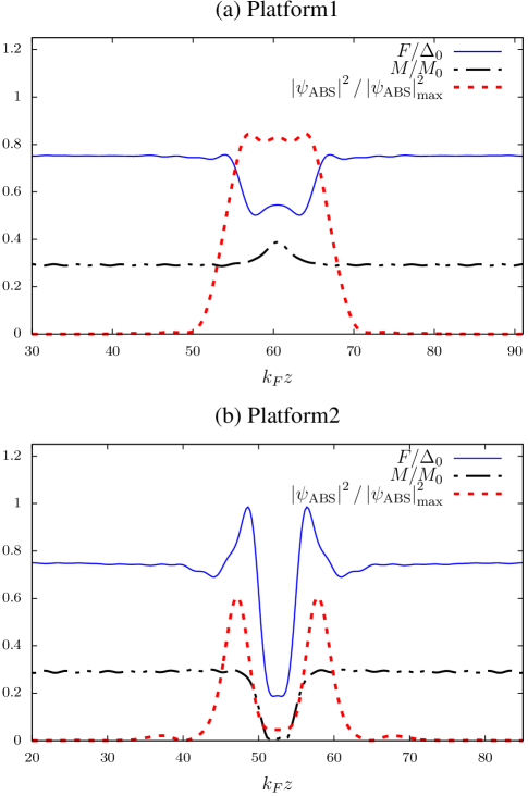
Figure 4: Plots for the pair amplitude, the magnetization, and the amplitude of $E=0$ bound state wave function as a function of position $z$ corresponding to the first and second platforms and with the parameters chosen from Figs. 2 and 3, respectively. Here we look at fixed $k_{F}y=2$ which is in the Ho layer. The bound state in platform 1 is non-topological while that in platform 2 can be shown to be associated with Majorana zero modes.

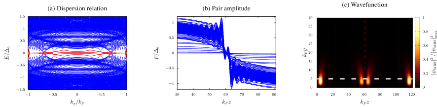
Figure 5: Results for the first platform when $\phi=\pi$. Other parameters are the same as in Fig. 2. The left panel shows the dispersion relation. The two Majorana edge modes are present and now become degenerate with two additional “Andreev” modes (as shown by the red lines near the zero energy). [These were visible in Fig. 2(a) where they were not quite degenerate.] The self-consistent pair amplitudes, plotted in the central panel, show a clear sign change in the insulator. The horizontal axis corresponds to the $z$-direction and each curve in this plot is a line cut along $y$-coordinates. In the right panel, we plot the wavefunction associated with $k_{x}=0.93k_{F}$ where there are two Majorana edge modes and two Andreev modes leading to the $4\pi$ Josephson effect. The boundary between the S layers and the Ho layers is represented by dashed lines.

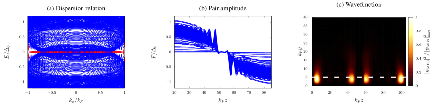
Figure 6: Results for the second platform when $\phi=\pi$. Other parameters are the same as in Fig. 3. The figure shows, from left to right: (a) the dispersion relation, (b) the pair amplitudes, and (c) the wavefunction. As in the first platform, note the sign change in the pair amplitude as shown in panel (b). Panel (c) shows the wavefunction at $k_{x}=0.96k_{F}$ corresponding to one of the four-fold degenerate Majorana edge modes [red lines in panel (a)].

The pair amplitude profile is shown as a color contour plot in Fig. 3(b). Here the insulating component has an essentially negligible pair amplitude. Similarly one sees from Fig. 3(c) that the magnetization is fully absent over the insulator, but once inside the Ho it turns on rather abruptly. The region of magnetization inhomogeneity corresponds to the vicinity of the Ho-I boundary on either side. If we then plot the amplitude of the crossing wavefunction as in Fig. 3(d), we see that it is essentially localized to this inhomogeneous region, with very small penetration into the superconducting leads.

Figure 4 presents line cuts in the Ho region of the contours shown in the different panels (b,c,d) of the previous two figures. Here the plots are for a fixed $y$ position in the junction. The upper and lower panels correspond to the first and second platforms, respectively. All curves are for dimensionless units; by overlaying them in this fashion one can see more clearly how the location of the zero-energy bound states is in detail correlated with the inhomogeneities in $\bf{m}(\bf{r})$ and $F({\bf r})$. Additionally, one can more directly compare the behavior in the first and second junction configurations. This enables a comparison between trivial and topological zero energy crossings.

In the upper panel, one sees that as the insulator is approached, the pair amplitude decreases while concomitantly the size of the magnetization increases in precisely the same spatial region. We have observed (not shown here) the expected inverse relationship between the size of the oscillations in the $x$ and $y$ components of $\bf{m}(\bf{r})$ and the size of the pair amplitude $F({\bf r})$. The zero-energy bound state is, as emphasized above, confined to the region of inhomogeneity.

The situation for the second platform (shown in the lower panel) is more complex. Note that the insulator is nearly “inert”,that is, it has a very small pair amplitude and very weak oscillating magnetism. Hence, by contrast with the upper panel, the entire central region of the plots is nearly zeroed out. As a consequence the bound state (hybridized Majorana) wavefunction is restricted to a region of width comparable to that in the first platform, but with the central region replaced by a “hole” across the extent of the insulator.

III.1 Topological Josephson junctions

We turn now to junctions with a $\pi$-phase difference between two superconducting leads. We stress that the Josephson current of a topological and trivial Josephson junction has different periodicity with respect to the superconducting phase difference, i.e., $4\pi$ periodicity for topological vs $2\pi$ periodicity for trivial junctions. This difference in the periodicity can be used as an experimental signature for the topological superconductivity. Importantly, one cannot differentiate between topological and trivial Josephson junction from the amplitude of the Josephson current.

Of particular interest here is to see the extent to which a proximitized junction (which has a vanishing order parameter) can, nevertheless, exhibit Josephson signatures. The behavior for the two different platforms is not dramatically different. Figures 5(a) and 6(a) present a plot of the energy dispersion as a function of $k_{x}$ for the first and second platforms, respectively. There are two notable effects as compared to junctions when both superconductors have the same phase: the excitation gap is significantly reduced and the flat bands at the edge are now four-fold degenerate. This four-fold degeneracy (associated with the low-energy states outlined in red) appears when the two bands just above and below the flat bands [these are shown at the edges of the spectrum in Figs. 2(a) and 3(a)] move down to align with the two Majorana flat bands. This occurs precisely when the phase difference reaches $\pi$. There are many more subgap states in Fig. 5 than Fig. 6 because in platform 2 the insulating region is more extended thereby leading to denser low-energy states.

It is useful to label the energies of these two near-by bands as $\pm E(\phi)$ and follow their behavior as the phase difference continuously varies. Note that these two have different fermion parity. When $\phi$ is less than $\pi$ the band associated with $+$ is above that with $-$. For angles between $\pi$ and $3\pi$, the two bands exchange places, with the $-$ band having higher energy that the $+$ band. At $3\pi$ the two bands will cross again at zero energy.

Using $E(\phi)$ we are able to predict the behavior of the Josephson current  Lutchyn et al. (2010); Oreg et al. (2010); Peng et al. (2016); Cayao et al. (2017). It follows that (unless there is a fermion-parity switch), the Josephson current will not return to its $\phi=0$ value until $\phi=4\pi$. This $4\pi$ periodicity is a well known feature of such junctions  Kitaev (2001); Fu and Kane (2009) and a signature of topological order. What is new here is these effects occur in a medium which has no intrinsic pairing. They are occuring strictly via proximity coupling.

Indeed, this proximity coupling is illustrated in Figs. 5(b) and 6(b) which plot the position-dependent pair amplitude for different values of $y$. This shows the expected sign change as one crosses from one superconductor to another. To accomodate this overall sign switch there appear to be distinct nodal points. Finally, Figs. 5(c) and 6(c) present contour plots of the wavefunction amplitudes associated with the four-fold degenerate flat bands at fixed $k_{x}=0.93k_{F}$ and $k_{x}=0.96k_{F}$, respectively. The two spots on the left and right are the expected Majorana bound states (MBSs) coming from the far edges of Ho, while the two in the middle correspond to the localized wavefunctions associated with the middle two edges of the Ho substrate. These are sometimes described as hybridized Majorana modes Lee et al. (2014b). Indeed, one can view the $4\pi$ periodicity discussed above as arising from these hybridized modes.

What is particularly interesting in the first platform configuration is that even though here there is no natural junction in the middle of the Ho substrate, the wavefunction nevertheless exhibits a break into two separate contributions, as in platform 2.

IV Assessing Standard Proximity Models: One dimensional junctions

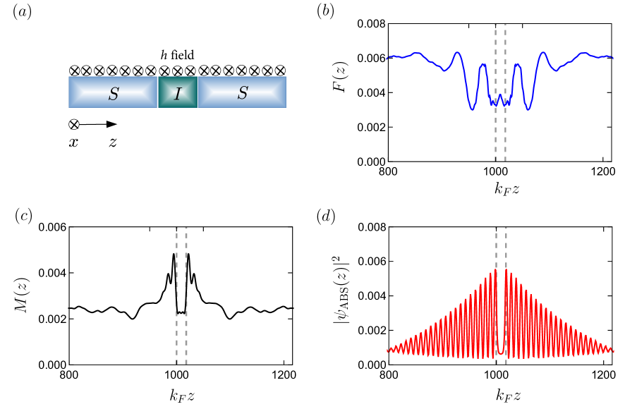
Figure 7: (a) Schematic arrangement of the effective low energy proximity model corresponding to Platform 1, (b) pair amplitude profile $F(z)$, (c) profile of total magnetization $M(z)$ and (d) the zero-energy bound state wave function which roughly correlates with the induced magnetization. The dashed lines in panels (b)-(d) mark the boundaries between the superconducting and insulating regions. This figure can be compared with Fig. 4(a). The parameters used in the above plots are $t_{\perp}=1.5$, $\ell_{S}=157\xi$, $\ell_{I}=2.5\xi$, $\Delta=0.1$, $\phi=0$, $\mu_{S}=1$, $\mu_{I}=-1$, $\lambda_{S}=0.2$, $\lambda_{I}=0.2$, $h_{S}=0.6$, and $h_{I}=0.6$.

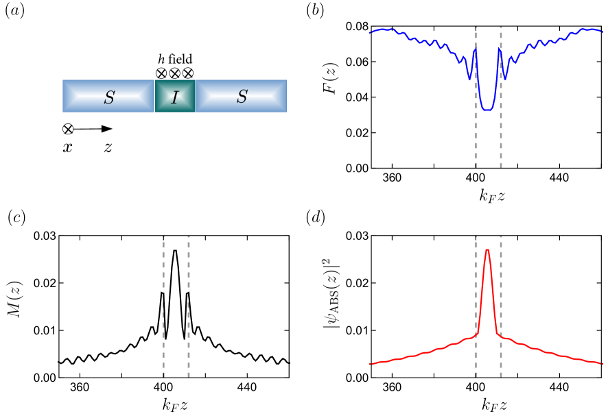
Figure 8: (a) Schematic arrangement of a 1D “trivial phase” junction with magnetic field only in the insulating region. This case is not related to either of the two platforms in Figure 1, but is presented to illustrate how the bound state wavefunctions are localized to regions with non-zero magnetic field. (b) Pair amplitude profile $F(z)$, (c) Profile of total magnetization $M(z)$ and (d) zero-energy bound state wave function which has an amplitude maximum where the magnetization is maximal. This case is non-topological, as there are no magnetic fields in S. The dashed lines mark the boundaries between the superconducting and insulating regions. The parameters used in the above plots are $t_{\perp}=1.5$, $\ell_{S}=60\xi$, $\ell_{I}=1.57\xi$, $\Delta=0.1$, $\phi=0$, $\mu_{S}=1$, $\mu_{I}=-1$, $\lambda_{S}=0.5$, $\lambda_{I}=0.5$, $h_{S}=0$, and $h_{I}=0.6$

A deep understanding of the nature of proximity-induced superconductivity in systems with combined spin-orbit coupling and Zeeman fields is central to arriving at topological superconductors. Rather than introducing the source of proximitization directly as we do here, one usually ignores the multiple layers of Figure 1, and considers an effective SIS system with an assumed gap parameter in S. In a nice series of papers, Stanescu and co-workers Sau et al. (2010); Stanescu et al. (2010); Stanescu and Das Sarma (2017); Stanescu et al. (2011) developed this approach. They showed how to derive an effective low energy model in which the superconducting degrees of freedom can be integrated out and replaced by an interface self energy.

Implementing their approach for the 2 different platforms leads to 2 different quasi-one dimensional models which (unfortunately) also need to be addressed numerically. Important here is to make these simpler models compatible with our Holmium studies by choosing a one-dimensional spin-orbit coupling. This can be shown to host Majorana flat bands in the topological regime. Moreover, as shown below, we find multiple parity switches associated with ZECs in the SIS spectrum.

Notably, these always require a sufficiently strong magnetic field to be present inside the insulator. We, thus, presume throughout this section that there is a non-zero field in the insulating region. It can be noted that this appears to be (at least) a superficial difference between these effective low energy models and the platform configurations discussed in the previous section, where no magnetic field is present in the actual insulating component of the junction; moreover, this region is relatively free of any magnetization [as can be seen in Figs. 2(c) and 3(c)]. Similarly the insulator does not host the zero-energy bound states in contrast to what is found in the effective low energy models. Rather the Holmium substrate is the active component in the junction (just below the insulator) hosting both the magnetization and the bound state.

In the following, we focus on the effective low energy model which involves 1D spin-orbit-coupled superconducting wires Lutchyn et al. (2010); Oreg et al. (2010) coupled infinitely along one direction (which we take to be the $x$-direction) Wang et al. (2014). Here we consider the system to be infinitely thin along the $y$-direction as shown in Fig. 7(a). Similar SIS and SNS junctions have been studied in the literature Cayao et al. (2015) which argue that for sufficiently large Zeeman fields, parity crossings are made possible by the nontrivial topology in the underlying effective $p$-wave superconductor. Here we find that these ZECs can also arise in the absence of SOC, hence they are not associated with topological phases.

IV.1 Effective low-energy models for including proximity

We next study the effective low-energy approximation to the full-proximitized SIS junction introduced in the previous section, namely an array of 1D finite-length (along $z$-direction) spin-orbit-coupled superconducting wires Lutchyn et al. (2010); Oreg et al. (2010) which are coupled along the infinite $x$-direction Wang et al. (2014). This effective low energy model is obtained by removing the two superconductors above the Holmium. Following the standard procedure for addressing proximity effects Sau et al. (2010); Stanescu et al. (2010); Stanescu and Das Sarma (2017); Stanescu et al. (2011), we integrate out the upper (SIS) layer which results in a contribution of a surface self energy in the Hamiltonian of Holmium. The self-energy is given by

$$\Sigma(\omega)=-|\widetilde{t}|^{2}\nu\left(E_{F}(z)\right)\left[\frac{\omega\tau_{0}+\Delta_{0}(z)\sigma_{y}\tau_{y}}{\sqrt{\Delta_{0}(z)^{2}-\omega^{2}}}+\frac{\zeta}{1-\zeta^{2}}\tau_{z}\right],$$ (4.1)

where $\widetilde{t}$ is the tunneling coupling between the SIS layer and Holmium, $\Delta_{0}$ is the parent superconductivity, $\nu(E_{F})=2\sqrt{1-\zeta^{2}/\Lambda}$ is the density of states at the Fermi energy $E_{F}$ with $\zeta=[\Lambda-E_{F}(z)]/\Lambda$ and $\Lambda$ being half of the bandwidth. The second term in Eq. (4.1) gives rise to the proximity-induced superconductivity and the last term introduces a shift in the chemical potential of the substrate. In this way we have an effective low-energy model for the Holmium component where the region below the host superconductor is a proximitized superconductor while that below the insulating barrier is treated as an insulator in a magnetic field, as shown in Fig. 7(a). This self-energy can be thought of as a consequence of the penetration of the wave function from the upper layer SIS part into the Holmium substrate. Since we are only interested in the zero-energy bound states which are the low-energy properties of the system, we can approximate $\Sigma(\omega)\approx\Sigma(0)$.

The Hamiltonian of the effective low-energy model of the Holmium is then given by

$$\mathcal{H}_{1D}= \int dz\left[\left(-\frac{\partial_{z}^{2}}{2m}-\mu(z)\right)+H_{\mathrm{\parallel}}\right.$$

$$\hskip 28.45274pt\left.+\left(\Delta(z)\psi^{\dagger}_{\uparrow}(z)\psi_{\downarrow}^{\dagger}(z)+\mathrm{H.c.}\right)\right],$$ (4.2)

where $\psi_{\sigma}(z)[\psi^{\dagger}_{\sigma}(z)]$ is the annihilation (creation) operator of an electron at position $z$ with spin $\sigma=\uparrow,\downarrow$ and $\Delta(z)=|\widetilde{t}|^{2}\nu(E_{F})\theta(\Delta_{0}(z))$ is a proximity-induced $s$-wave pairing potential.

Note that the chemical potential $\mu(z)$ and pairing potential $\Delta(z)$ vary along the $z$ direction [see Fig. 7(a)] where $\mu_{I}<0$, $\mu_{S}>0$, $\Delta_{S}>0$, and $\Delta_{I}=0$. In the above, we have used the subscripts I and S to denote the quantities corresponding to the I and S regions, respectively in Fig. 7(a).

The term

$$H_{\mathrm{\parallel}}= -i\lambda\left(\psi^{\dagger}_{\uparrow}(z)\psi_{\uparrow}(z+\hat{z})-\psi^{\dagger}_{\downarrow}(z)\psi_{\downarrow}(z+\hat{z})\right)+\mathrm{H.c.}$$

$$+h\left(\psi^{\dagger}_{\uparrow}(z)\psi_{\downarrow}(z)+\psi^{\dagger}_{\downarrow}(z)\psi_{\uparrow}(z)\right),$$ (4.3)

contains the spin-orbit ($\lambda$) and Zeeman ($h$) coupling. Note that this nanowire Hamiltonian is equivalent to the proximity-induced superconducting ferromagnet at a conical opening angle $\alpha=\pi/2$ Wu et al. (2017) as discussed in the previous section.

We introduce a coupling in the array of the 1D wires along the $x$-direction via the term

$$H_{\perp}=-t_{\perp}\int dx\left[\psi^{\dagger}(x,z)\psi(x+\hat{x},z)+\mathrm{H.c.}\right].$$ (4.4)

Here we have defined $\hat{x}$ and $\hat{z}$ to be the unit vectors along the $x$ and $z$ directions, respectively. Since the Hamiltonian is translationally invariant along the $x$-direction, the Hamiltonian of the above 2D system can be dimensionally reduced into a sum of 1D wires each with specific values of $k_{x}$, i.e.,

$$\mathcal{H}_{\mathrm{2D}}=\int dk_{x}\mathcal{H}_{\mathrm{1D}}(k_{x}).$$ (4.5)

where $\mathcal{H}_{1D}(k_{x})$ is the same as Eq. (IV.1) written in momentum space with the chemical potential replaced by $\mu\rightarrow\widetilde{\mu}(k_{x})=\mu+2t_{\perp}\cos(k_{x})$. When the magnetic field is tuned above its critical value $h>|\Delta|$, the superconducting region of the array of 1D wires can support any integer $Z$ gapless Majorana zero modes thus it belongs to the topological class BDI Schnyder et al. (2008); Kitaev (2009); Tewari and Sau (2012). For $h<|\Delta|$, the system is in the trivial phase and gapped. The gap closes when $h>|\Delta|$ where the system becomes topological with Majorana flat bands in the $E$ versus $k_{x}$ spectrum. These Majorana flat bands can be found in the $k_{x}$ region where $h^{2}>\widetilde{\mu}(k_{x})^{2}+\Delta^{2}$. We note that the gap closes at the $k_{x}$ values where $\widetilde{\mu}(k_{x})^{2}+\Delta^{2}=h^{2}$. For the case where $|\sqrt{h^{2}-\Delta^{2}}-|\mu||\leq 2t_{\perp}\leq(|\mu|+\sqrt{h^{2}-\Delta^{2}})$, there are two gap closing points and for the case where $|\mu|+\sqrt{h^{2}-\Delta^{2}}\leq 2t_{\perp}$, there are four.

IV.2 Numerical Results: Effective low-energy models

We focus on numerical solutions of the BdG equations given in Eqs. (IV.1)-(4.5). In particular, we compute the zero-energy bound state wavefunction, proximitized gap [Eq. (1.23)], and magnetization [Eq. (1.24)]. Importantly, here, too, we find ZECs in the spectrum which signify QPTs.

In Figs. 7(a)-(d) we present solutions of the effective low energy model corresponding to Platform 1. Here, the insulating region has a constant negative chemical potential $\mu_{I}<0$ with a length $\ell_{I}\sim\xi$ where $\xi=2/(\pi\Delta)$ is the superconducting coherence length with $\Delta$ being the superconducting gap. Multiple zero energy bound states of the effective model are found to appear once the Zeeman field in the insulating region of an SIS junction is increased to the critical value ($h_{I}=|\mu_{I}|$), where $\mu_{I}$ is the chemical potential in I.

Figure 7(a) shows the junction configuration where the magnetic field is naturally present in the insulating region. The pairing potentials on the left and right superconducting regions are taken to be $\Delta$ and $\Delta e^{i\phi}$, respectively. For simplicity, the results here are presented for the case $\phi=0$.

To relate to our more complete proximity calculations, we plot the associated pairing amplitudes $F({\bf r})$, [see Fig. 7(b)], the magnetization [see Fig. 7(c)] and (for one particular bound state) the zero-energy wavefunction amplitude as functions of position throughout the junction [see  7(d)]. This figure can then be compared with Fig. 4(a). Just as in Fig. 4(a), the magnetization and the wavefunction amplitude are correlated with each other: they assume their maximum values at the same position. One can compare with Fig. 4(a) where the counterparts from the full proximity calculation exhibit a maximum in the junction center, whereas in Fig. 7, they both have minima. The pairing amplitudes shown in Fig. 4(a) and in Fig. 7(b) are more obviously similar, as they both exhibit a dip in the center of the junction. It should be noted, as can be seen from the plot, the pairing penetrates into the insulator.

If the magnetic field is absent in the I region of the effective low energy model, then the non-topological zero energy bound states are no longer present. This case, which would be associated with platform 2, does not yield a discrete zero energy crossing in the dispersion as in the full proximity case of Fig. 2(a). Rather it is associated with a Majorana flat band. In this way, we infer that these effective low energy models do not always accomodate the same detailed physics as in a more realistic proximity junctions.

Finally, we present results in Fig. 8 for a simple case of a trivial SIS junction where the superconductor contains SOC but no magnetic field. For this configuration the magnetic field is restricted to be inside the insulating region. This case is unrelated to the 2 holmium platforms considered throughout the paper. Nevertheless, it serves to illustrate the importance of a non-zero Zeeman field in hosting non-topological quantum phase transitions. We have seen in the second platform configuration (Figures 3 and 4(b)) that the bound state wave function is essentially excluded from regions in the junction where the field vanishes. Thus the wave function does not overlap the insulating region. We see in Figure 8 a similar effect. Here, again following the behavior of the magnetic field, the bound state wave function is essentially confined to the insulating region and excluded from the host superconductors where the field vanishes.

We note that this case is closer to that studied in Refs. Liu et al. (2017); Cayao et al. (2015). What is particularly intriguing about this situation is that it can be thought of as a “quantum dot” system where Coulomb blockade effects are absent. Generally the presence of Coulomb blockade physics is used Kiršanskas et al. (2015) to argue that Kondo physics is driving the QPT in quantum dots. This follows by using a Schrieffer-Wolff transformation to convert the dot Hamiltonian to a magnetic impurity model. What is shown here and in Ref. Liu et al. (2017) is that Coulomb effects are not essential for arriving at these quantum phase transitions in quantum dots.

The junction configuration of interest is shown in Figure 8(a) whereas Figure 8(b) presents a plot of the self-consistent pair amplitude calculated using Eq. (1.23). As can be seen from the plot, the gap penetrates into the insulator. Figure 8(c) shows the magnetic screening cloud or magnetization $M(z)$ throughout the junction with its components calculated using Eq. (1.24). The magnetization is largest in the insulating region as a consequence of the magnetic field there. Finally in Figure 8(d) we present a plot of the amplitude of the wavefunction corresponding to a prototypical zero-energy bound [$\psi_{\mathrm{ABS}}(z)$]. We see that the magnetization and the wavefunction are spatially correlated and peaked in the insulating regime, reflecting the presence of the magnetic field which only appears in this region.

V Conclusions

V.1 Comparison of the full proximity results with the effective model

It is interesting to focus on the behavior in the vicinity of the various interfaces in the complex Josephson junctions we consider. Note that the S-Ho interface is effectively absent in the low energy models used for addressing proximity coupling (see Section IV, where the contribution from S has been integrated out.) On the otherhand, it is accessible in the full proximity calculations and both Figs. 2 and 3 show that the induced magnetization barely penetrates into the superconducting region. This is due to the fact that the exchange interaction is local and present only in the Ho layer Bergeret et al. (2005). Rather the magnetization is confined to Ho. In platform 2 it is locally depressed in the insulating region, where Ho is completely absent; it, nevertheless, recovers to the full bulk value associated with Ho at the sample ends far from the insulator. By contrast in platform 1 the magnetization is increased in the vicinity of (but below) the insulator, acting much as a local magnetic moment.

The pair amplitude undergoes a more non-monotonic behavior associated with the S-Ho interface which is missing in the low energy approximate models. These oscillations are well known (see, for example Wu et al. (2012)). In this way there is a depression in the pairing amplitude very close to the S-Ho interface, but it recovers to become rather strong somewhat below. Importantly, the wavefunctions for the QPT in Platform 1 are localized in Ho in the regime where the pairing amplitude is maximal.

At some level there is consistency between the effective models and the full proximity calculations, as we find in platform 1 (through both approaches) that there are non-topological zero energy crossings. Similarly we find in platform 2 (through both approaches) that the crossings there are only topological. What is important to stress, however, is that the full proximity models are more complete because they self consistently establish the degree and even the presence of proximitization. In the effective models one usually introduces a phenomenological pairing gap parameter $\Delta$ as in Eq. (IV.1), whose size can only be obtained from the full proximity calculations. We emphasize this size is critical in determining the conditions for topological and trivial phases. These differences are also made clear by contrasting Figs. 4(a) and 7.

V.2 Physical Picture of the quantum phase transition

By way of summary, it is useful to revisit the question of what is the physical mechanism responsible for these non-topological zero energy bound states found in either the full proximity Josephson case or with the effective low energy model. We have shown throughout that there is a clear correlation between the inhomogeneous magnetization and the amplitude of the bound state wavefunction. We associate a proximity-induced “magnetic defect” with the insulating region of the junction. In the presence of magnetic fields, the insulator effects a local reorganization of the magnetization in the proximitized medium. We emphasize that our insulating barriers are non-magnetic. The proximity-induced “magnetic” defects which we refer to as magnetization inhomogeneities, have a different origin from the well-studied magnetic impurities associated with the Shiba scenario Shiba (1968).

Nevertheless these Shiba or “external” impurities provide a useful template for understanding zero-energy crossings. These crossings are found to occur by tuning the strength of the effective impurity exchange interaction Yu (1965); Shiba (1968); Sakurai (1970). Using this template in the present situation, it is the magnetic field (in units of the insulating chemical potential) which provides a mechanism for the energy level crossings and parity shifts in our proximitized Josephson junctions. At a critical magnetic field the energies of the superconducting junction states with $n$ and $n+1$ electrons cross. The parity switch of the crossing reflects the fact that in a region of rapidly varying magnetization it may be energetically more favorable to invert the relative order of different states (having different parities). This is implemented by adding an additional fermion spin or single particle excitation, associated with one less pair and one extra spin.

It is useful to contrast our effective low energy proximity model results with the case of a delta-function non-magnetic impurity studied in Ref. Sau and Demler (2013). The present picture applies to a finite-length insulating barrier and we find that this zero-energy crossing can appear as long as the magnetic field in the insulating region is sufficiently large ($h_{I}>|\mu_{I}|$).The crossings we find do not require the superconducting region to be topological, as in Ref. Sau and Demler (2013). Similarly, there are studies of multiple magnetic impurities, or impurity chains in the literature Björnson et al. (2017). While we also consider magnetization defects of extended size, ours are not externally inserted but are proximity-induced through full self consistency. They arise because of the presence of magnetic fields in (proximitized) superconductors, which, around an insulating barrier, serve to induce an inhomogeneous magnetization.

Finally we note that there is a literature which is closer to the issues presented in the present paper. This deals with Andreev bound states in the presence of magnetic fields Liu et al. (2017); Cayao et al. (2015). The (necessarily) numerical findings from this body of work show how these bound states appear as functions of junction magnetic field and chemical potentials but without establishing detailed microscopic governing equations. Indeed, it has been argued both theoretically Cayao et al. (2015) and experimentally Lee et al. (2017) that there are similarities between Andreev bound states and those associated with magnetic impurities. A notable contribution from the present paper was to present a “missing link” which explains the similarity. We did this by identifying the role of the proximity-induced magnetization $\bf{m}(\bf{r})$ arising in an Andreev configuration, which is something which was previously of interest only to the superconducting spintronics community.

V.3 Summary

In this paper we addressed fairly realistic proximitized Josephson junctions which contain the necessary features (both Zeeman and spin-orbit coupling) to produce topological superconducting phases. While we have focused on a particular example involving the conical magnet Ho, we expect our findings to be more general. These junctions contain multiple non-topological zero-energy bound states associated with fermion-parity switches in quantum phase transitions. They are particularly important because they have the potential to lead to “false positives” in reports for Majorana bound states. Thus, understanding their origin more microscopically provides a central motivation for our work here.

To understand these quantum phase transitions, we have presented a full proximity treatment of multi-component Josephson junctions. Despite the many papers concerned with topological junctions, a detailed and precise proximity analysis appears to be otherwise lacking. It, moreover, provides a valuable check on widely used effective low energy models which we examine here. We show how it is useful to consider self-consistently derived quantities from the BdG analysis such as the screening cloud magnetization $\bf{m}(\bf{r})$, and induced pairing amplitudes $F({\bf r})$. These allow us to understand the appearance of zero-energy bound states and to correlate their areas of confinement to the spatial dependences of these properties. In this way, we arrive at a generalization of the magnetic impurity scenario for these quantum phase transitions, but here with a self consistent and proximity-induced magnetic defect.

Acknowledgements.– We thank Erez Berg, Shinsei Ryu, J. Robinson, Alexa Galda, Jay Sau and Michael Levin for helpful conversations. This work was supported by NSF-DMR-MRSEC 1420709. C.-T.W. is supported by the MOST Grant No. 106-2112-M-009-001-MY2C. We acknowledge the University of Chicago Research Computing Center for support of this work.

References

- Sau and Demler (2013) J. D. Sau and E. Demler, Phys. Rev. B 88, 205402 (2013).
- Cayao et al. (2015) J. Cayao, E. Prada, P. San-Jose, and R. Aguado, Phys. Rev. B 91, 024514 (2015).
- Lee et al. (2017) E. J. H. Lee, X. Jiang, R. Žitko, R. Aguado, C. M. Lieber, and S. De Franceschi, Phys. Rev. B 95, 180502 (2017).
- Peng et al. (2015) Y. Peng, F. Pientka, Y. Vinkler-Aviv, L. I. Glazman, and F. von Oppen, Phys. Rev. Lett. 115, 266804 (2015).
- Chang et al. (2013) W. Chang, V. E. Manucharyan, T. S. Jespersen, J. Nygård, and C. M. Marcus, Phys. Rev. Lett. 110, 217005 (2013).
- Sau et al. (2010) J. D. Sau, R. M. Lutchyn, S. Tewari, and S. Das Sarma, Phys. Rev. B 82, 094522 (2010).
- Stanescu et al. (2010) T. D. Stanescu, J. D. Sau, R. M. Lutchyn, and S. Das Sarma, Phys. Rev. B 81, 241310 (2010).
- Stanescu and Das Sarma (2017) T. D. Stanescu and S. Das Sarma, Phys. Rev. B 96, 014510 (2017).
- Stanescu et al. (2011) T. D. Stanescu, R. M. Lutchyn, and S. Das Sarma, Phys. Rev. B 84, 144522 (2011).
- Hell et al. (2017) M. Hell, M. Leijnse, and K. Flensberg, Phys. Rev. Lett. 118, 107701 (2017).
- Yu (1965) L. Yu, Acta Phys. Sin 21 (1965).
- Shiba (1968) H. Shiba, Progress of theoretical Physics 40, 435 (1968).
- Sakurai (1970) A. Sakurai, Prog. Theor. Phys. 44, 1472 (1970).
- Linder and Robinson (2015) J. Linder and J. W. A. Robinson, Nature Physics 11, 307 (2015).
- Bernardo et al. (2015) A. Bernardo, S. Diesch, Y. Gu, G. Divitini, D. Ducati, E. Scheer, M. G. Blamire, and J. W. A. Robinson, Nature Comm. 6, 8053 (2015).
- Liu et al. (2012) J. Liu, A. C. Potter, K. T. Law, and P. A. Lee, Phys. Rev. Lett. 109, 267002 (2012).
- Bagrets and Altland (2012) D. Bagrets and A. Altland, Phys. Rev. Lett. 109, 227005 (2012).
- Pikulin et al. (2012) D. I. Pikulin, J. P. Dahlhaus, M. Wimmer, H. Schomerus, and C. W. Beenakker, New Jour. of Phys. 14, 125001 (2012).
- Wu et al. (2017) C.-T. Wu, B. M. Anderson, W.-H. Hsiao, and K. Levin, Phys. Rev. B 95, 014519 (2017).
- Kiršanskas et al. (2015) G. Kiršanskas, M. Goldstein, K. Flensberg, L. I. Glazman, and J. Paaske, Phys. Rev. B 92, 235422 (2015).
- Lee et al. (2014a) E. J. H. Lee, S. Jiang, M. Houzet, R. Aguado, and L. C. M, Nature Nanotechnology 9, 79 (2014a).
- Deacon et al. (2010) R. S. Deacon, Y. Tanaka, A. Oiwa, R. Sakano, K. Yoshida, K. Shibata, K. Hirakawa, and S. Tarucha, Phys. Rev. Lett. 104, 076805 (2010).
- Alicea (2012) J. Alicea, Rep. Prog. Phys 75, 076501 (2012).
- Beenakker (2013) C. W. Beenakker, Ann. Rev. Condens. Phys. 4, 113 (2013).
- Elliott and Franz (2015) S. R. Elliott and M. Franz, Rev. Mod. Phys. 87, 137 (2015).
- Li et al. (2016) J. Li, T. Neupert, Z. Wang, A. H. MacDonald, Y. Yazdani, and A. Bernevig, Nature Communications 7, 12297 (2016).
- Li et al. (2014) J. Li, H. Chen, I. K. Drozdov, A. Yazdani, B. A. Bernevig, and A. H. MacDonald, Phys. Rev. B 90, 235433 (2014).
- Mourik et al. (2012) V. Mourik, K. Zuo, S. M. Frolov, S. R. Plissard, E. P. Bakkers, and L. P. Kouwenhoven, Science 336, 1003 (2012).
- Deng et al. (2016) M. T. Deng, S. Vaitiekenas, E. B. Hansen, J. Danon, M. Leijnse, K. Flensberg, J. Nygard, P. Krogstrup, and C. M. Marcus, Science 354, 1557 (2016).
- Liu et al. (2017) C.-X. Liu, J. D. Sau, T. D. Stanescu, and S. Das Sarma, Phys. Rev. B 96, 075161 (2017).
- Klapwijk (2004) T. M. Klapwijk, Jour. of Superconductivity 17, 593 (2004).
- Halterman and Valls (2001) K. Halterman and O. T. Valls, Phys. Rev. B 65, 014509 (2001).
- Halterman and Valls (2002) K. Halterman and O. T. Valls, Phys. Rev. B 66, 224516 (2002).
- Sticlet et al. (2017) D. Sticlet, B. Nijholt, and A. Akhmerov, Phys. Rev. B 95, 115421 (2017).
- Chiodi et al. (2013) F. Chiodi, J. D. S. Witt, R. G. J. Smits, L. Qu, G. B. Halasz, C.-T. Wu, O. T. Valls, K. Halterman, J. W. A. Robinson, and M. G. Blamire, EPL 101, 37002 (2013).
- Halász et al. (2009) G. B. Halász, J. W. A. Robinson, J. F. Annett, and M. G. Blamire, Phys. Rev. B 79, 224505 (2009).
- Nadj-Perge et al. (2013) S. Nadj-Perge, I. K. Drozdov, B. A. Bernevig, and A. Yazdani, Phys. Rev. B 88, 020407 (2013).
- Martin and Morpurgo (2012) I. Martin and A. F. Morpurgo, Phys. Rev. B 85, 144505 (2012).
- Wu et al. (2012) C.-T. Wu, O. T. Valls, and K. Halterman, Phys. Rev. B 86, 184517 (2012).
- Cheng et al. (2009) M. Cheng, R. M. Lutchyn, V. Galitski, and S. Das Sarma, Phys. Rev. Lett. 103, 107001 (2009).
- Das Sarma et al. (2012) S. Das Sarma, J. D. Sau, and T. D. Stanescu, Phys. Rev. B 86, 220506 (2012).
- Lutchyn et al. (2010) R. M. Lutchyn, J. D. Sau, and S. Das Sarma, Phys. Rev. Lett. 105, 077001 (2010).
- Oreg et al. (2010) Y. Oreg, G. Refael, and F. von Oppen, Phys. Rev. Lett. 105, 177002 (2010).
- Peng et al. (2016) Y. Peng, F. Pientka, E. Berg, Y. Oreg, and F. von Oppen, Phys. Rev. B 94, 085409 (2016).
- Cayao et al. (2017) J. Cayao, P. San-Jose, A. M. Black-Schaffer, R. Aguado, and E. Prada, Phys. Rev. B 96, 205425 (2017).
- Kitaev (2001) A. Y. Kitaev, Physics-Uspekhi 44, 131 (2001).
- Fu and Kane (2009) L. Fu and C. L. Kane, Phys. Rev. B 79, 161408 (2009).
- Lee et al. (2014b) S.-P. Lee, K. Michaeli, J. Alicea, and A. Yacoby, Phys. Rev. Lett. 113, 197001 (2014b).
- Wang et al. (2014) D. Wang, Z. Huang, and C. Wu, Phys. Rev. B 89, 174510 (2014).
- Schnyder et al. (2008) A. P. Schnyder, S. Ryu, A. Furusaki, and A. W. W. Ludwig, Phys. Rev. B 78, 195125 (2008).
- Kitaev (2009) A. Y. Kitaev, AIP Conf. Proc. 1134, 22 (2009).
- Tewari and Sau (2012) S. Tewari and J. D. Sau, Phys. Rev. Lett. 109, 150408 (2012).
- Bergeret et al. (2005) F. S. Bergeret, A. F. Volkov, and K. B. Efetov, Rev. Mod. Phys. 77, 1321 (2005).
- Björnson et al. (2017) K. Björnson, A. V. Balatsky, and A. M. Black-Schaffer, Phys. Rev. B 95, 104521 (2017).