Algorithms for the explicit computation of Penrose diagrams
Abstract
An algorithm is given for explicitly computing Penrose diagrams for spacetimes of the form . The resulting diagram coordinates are shown to extend the metric continuously and nondegenerately across an arbitrary number of horizons. The method is extended to include piecewise approximations to dynamically evolving spacetimes using a standard hypersurface junction procedure. Examples generated by an implementation of the algorithm are shown for standard and new cases. In the appendix, this algorithm is compared to existing methods.
pacs:
04.20.Cv, 04.20.Gz-
January 2018
-
Keywords: general relativity, differential geometry, Penrose diagram, conformal diagram, null shell formalism
1 Introduction
Visualizing the causal structure of curved spacetime is among the basic tasks of relativistic physics. A useful tool in this pursuit, the technique now known as Penrose diagram analysis, in which finite coordinate diagrams of conformally transformed spacetimes are used to visualize global structure, was first introduced by Penrose in 1964 [1, 2]. The same technique was soon implemented by Carter [3], who was first to provide such diagrams in a recognizably modern form. An important systematic analysis was later given by Walker in 1970 [4]. The significance of these techniques as a tool to study asympototic infinities in spacetime was quickly recognized [5].
It is surprising, given the importance of Penrose diagrams, that one rarely sees a “real” one. They are almost always hand-drawn — in fact, it is rare even to find a computer-generated Penrose diagram of Minkowski space. There are some exceptions to this rule, including a number of especially nice diagrams due to Hamilton [6], and some others from Griffiths and Podolskỳ [7]. However, no general method for the numerical computation of diagrams across a broad and interesting class of metrics has been given. To do so is the goal of this article.
An algorithm will be given for constructing and numerically generating Penrose diagrams for spacetimes in two classes:
-
(A)
Maximally extended completions of spacetimes which locally have the form . (We refer to these spacetimes as strongly spherically symmetric (SSS), see section 4).
-
(B)
Piecewise-SSS spacetimes with null-shell junctions. These are constructed by joining pieces of spacetimes of class (A) across null shells of matter. These may have an arbitrary finite number of shells and piecewise regions.
This is achieved by adopting a global contour integral definition of the tortoise coordinate (see section 5), and making a careful choice of the function that squishes the local double-null coordinates (see sections 4 and 5) into the global coordinate patch. The result is a global double-null patch of “Penrose” coordinates (see section 2) in which the metric is continuous and non-degenerate at the horizons.
The new techniques we describe are similar in most respects to those used by Carter, Walker, and others. Our technique differs, however, by achieving simultaneous global coordinates for an arbitrary number of blocks across an arbitrary number of horizons, being numerically computable with weak restrictions on the metric function , and yielding diagrams whose lines of constant radius take on an intuitive shape. For a detailed comparison of the new and existing methods, see A.
There are a few reasons why Penrose diagrams have continued to be hand-drawn in the computer age, which is to say, why this algorithm has not been given sooner. Most importantly, the outline and qualitative appearance of Penrose diagrams for SSS spacetimes can be determined by the block diagram method of Walker [4]. When the diagram is being constructed primarily for analysis at infinity, the interior structure is irrelevant, and so the qualitative block diagram method is sufficient. Moreover, most known Penrose diagrams represent either vacuum spacetimes, or spacetimes with a homogeneous distribution of matter, making interior analysis rather dull. In contrast to these historical precedents, we wish to study diagrams for spacetimes which have nontrivial matter distributions, and which are dynamically evolving in nontrivial ways. The detailed interior appearance of such diagrams is not obvious from the standard qualitative analysis.
In particular, a major motivation for this endeavor is the desire to produce a detailed Penrose diagram for the process of black hole formation and evaporation, such that the distribution and flow of matter can be clearly and explicitly tracked. Fortunately, since class (B) above includes piecewise approximations to many interesting dynamically evolving geometries (e.g. Vaidya metric [7], forming and evaporating Hayward black hole [8], and stellar-collapse black hole models), the algorithms presented in this article will make that goal accessible.
An outline of the article is as follows.
Sections 2-4 serve two purposes. First, to review the well-known theory of Penrose diagrams in general and as applied to strongly spherically symmetric spacetimes. And second, to establish a clear and modern formalism in which to state the results of later sections. We hope that this formalism helps distill the key features of standard Penrose diagram analysis, and that these sections might be used as a pedagogical introduction to the subject for students with a strong background in differential geometry.
Sections 5-6 present new techniques for the practical construction of Penrose diagrams, while Section 7 describes an implementation of these techniques, and gives examples generated by the implementation. A gives a detailed comparison between existing methods and the new methods.
Some of the appendices may be of general interest. Readers interested in the symmetry of manifolds may enjoy C, which shows how spherical symmetry about a particular rotation axis can be defined, even when the symmetry axis is not itself a part of the manifold. B describes a useful unit convention for tensor components in relativity. And E collects a variety of useful geometric information about SSS spacetimes, including discussions of their trapped surfaces, physical singularities, and energy condition violations. The other appendices cover details particular to the text.
For those wishing to quickly see the practical algorithms we employ, the most direct route is to read section 5.4 followed by 6.2. The examples in figures 15 – 18, and the comparison to other methods in A, should also be consulted. Additionally, scanning figure 2 will help clarify the SSS spacetime terminology. This quick path through the paper is mostly, but not entirely, self-contained.
2 Penrose diagrams in two and more dimensions
We begin by reviewing the general theory of Penrose diagrams, and establishing a formalism commensurate with standard practices.
In general, the term “Penrose diagram” refers to a broad class of spacetime diagrams from which the causal structure of a spacetime can be easily read off. In particular, a Penrose diagram should make evident (i) the lightcone structure, and (ii) the causal structure of conformal infinity (defined below). This is typically achieved by covering a two-dimensional slice of a spacetime with a finite patch of double-null coordinates. Although most authors need not bother to have a rigorous definition of Penrose diagram in mind, it is possible to give a precise definition which is in line with typical use. We do so now for the case of two dimensions, and then discuss the generalization to higher dimensions.
2.1 Rigorous definition in two dimensions
Consider a two dimensional spacetime , and an open set . Let be a chart on , with coordinates for . Let denote the closure of , and let denote the image of in . Then may be called a Penrose chart if it satisfies three conditions: (I) ; (II) there exists a compact such that ; (III) in coordinates the metric takes the form , such that and , are both future-directed. When is a Penrose chart the coordinates may be called Penrose coordinates, and the boundary of the closure of is called the conformal boundary of . Any plot of in Penrose coordinates is called a Penrose diagram.
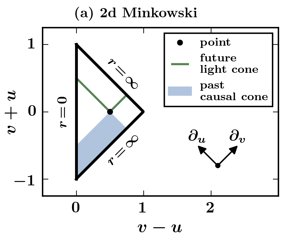
Condition (I) ensures111Sometimes has a periodic structure, in which case this condition can be weakened. Suppose consists of a periodic arrangement of regions isometric to . Then it suffices to require of a Penrose chart only that (I’) , so long as we specify how the regions are connected. This information is, of course, equivalent to knowing the global causal structure. Standard examples of the periodic case are the maximally extended Reissner-Nordstrom and Kerr (on axis) spacetimes [5]. that the diagram includes all of , while allowing some points to be left out to avoid technical difficulties (such as polar coordinate singularities) associated with attempting to cover all of in a single chart. Condition (II) ensures that the coordinate patch is finite, which allows the entirety of to be represented in a finite diagram, and allows analysis of the conformal boundary. And condition (III) ensures that the Penrose coordinates are double-null, making it trivial to identify lightcones and causal cones in the coordinates. Indeed, for any parameterized null curve , which implies that the curve follows lines of constant or (where dot represents a derivative with respect to curve parameter). This determines the lightcone at each point. The causal interior of the lightcone may then be determined by the condition for timelike curves. Because of these restrictions on the lightcones, a Penrose diagram is typically plotted with x-axis and y-axis . In such a case the lightcone is formed by rays at angles to the axes, with the top wedge being the future causal cone and the bottom wedge being the past causal cone (see Figure 1).
The conformal boundary of under , as defined above, plays a key role in understanding global causal structure because it allows the analysis of causal structure at “infinity”. The existence of a nonempty under a Penrose chart is guaranteed by condition (II) above. In general, points may be one of several types: (i) may represent points at “infinity”; (ii) if is incomplete at a curvature singularity, may represent the singularity; (iii) if is incomplete without curvature singularity, may represent a boundary where “missing” parts of are simply left out. When working in more dimensions (see below), there is an additional possibility that (iv) represents a coordinate boundary of the projection (e.g. ). In practice it is usually easy to distinguish between the various possibilities, and to identify the boundary set representing infinity. This set is called conformal infinity. Our definition of conformal boundary is similar to that originally set forth by Penrose [2]. The more common definition in terms of terminal indecomposable sets [9] is more general but less easily applicable when a Penrose chart exists.
In two dimensions, the Penrose chart describes a conformal isometry of into a subset of Minkowski space, when the coordinate space is equipped with metric . This allows the geometry of the boundary to be studied in the conformal Minkowski space, and is the reason for the term “conformal” boundary. Since conformal isometries preserve causal structure, studying in the conformal space determines the causal structure at infinity in . Determining this structure is one of the main goals of constructing a Penrose diagram for .
Practically speaking, the effort of constructing the Penrose diagram comes in two parts: (i) obtaining local double null coordinates; and (ii) manipulating the local patches to achieve a global double null coordinate system in which the metric is well-behaved (in the sense of condition (III)). Once (ii) has been achieved, it is trivial to (if necessary) squish and flip the global coordinates so as to attain Penrose coordinates. In sections 4 - 5 we will show for a certain class of spacetimes that (i) is trivial, and describe a method for resolving (ii). This method results immediately in Penrose coordinates.
2.2 Generalization to higher dimensions
How does this definition extend to higher dimesions? In the case of spherical symmetry, the theory goes through nearly unchanged. In this section, let have spacetime dimensions.
When spherical symmetry is present, a Penrose chart should be defined analogously to the two dimensional case, with the modification that for , with . Here represents a collection of angular coordinates, and the metric of an -sphere. The diagram is then constructed by defining the projective Penrose chart by and the projective metric . In this way, one essentially creates a Penrose diagram of the two dimensional spacetime transverse to the angular directions. Each point on the diagram represents a sphere of areal radius . It is important not to discard the radial information, as only by retaining the function can the geometry at each point of the diagram be specified.
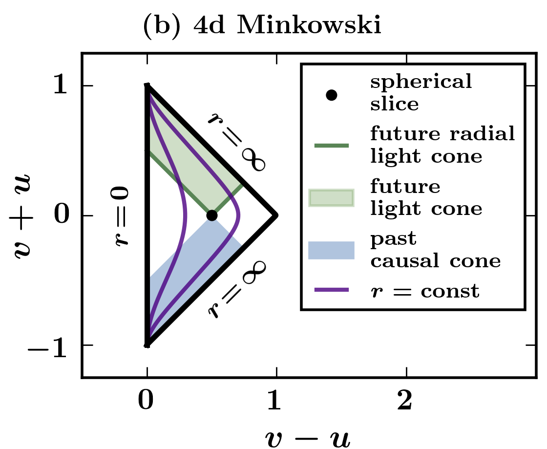
But even in case of spherical symmetry, the theory is slightly modified. The interpretation of the conformal space is no longer strict, since the coordinate Minkowski space is only conformal to after projection into two dimensions. The projection into two dimensions also has the effect that the appearance of lightcones in the diagram is qualitatively altered. Null curves in dimensions obey , while timelike curves obey . Thus, two-dimensional null curves in the confomal Minkowski space now represent only the radial null curves in , while -dimensional null curves with angular momentum in appear timelike in the conformal space. The -dimensional lightcones of , therefore, fill the interior of the two-dimensional causal cones in the conformal space. Despite these several modifications to the interpretation of the conformal space, the conformal method for studying infinity remains useful, and the name conformal boundary is retained.
For most of our purposes it will be convenient to deal with spherically symmetric shells and particles constrained to move in the plane. It is therefore useful to identify the radial lightcones, defined by , which are the effective lightcones for such objects. The -dimensional radial lightcones are equivalent to the two-dimensional conformal lightcones. Radial causal cones can be defined similarly. This concludes the extension from two dimensions to spherical symmetry in dimensions.
In some cases the spherically symmetric formalism can be generalized further. Let be a two-dimensional Lorentzian manifold with line element , and let be a positive real scalar function on . Let be an -dimensional homogeneous Riemannian manifold with line element . If there exist such an and for which a dense open submanifold is isometric to the product with metric , then a formalism directly analogous to that for spherical symmetry can be used (although if is not compact, condition (II) should be modified to apply only to the projective chart , and one should be careful in interpretation). This includes cases of planar, hyperbolic, and spherical symmetry, among others. The above condition implies that has at least spacelike Killing vector fields, and is essentially equivalent to the condition that can be acted on by an -dimensional group of spacelike isometries.
When lacks sufficient symmetry for analogous methods to be applied, by having nontrivial geometry in more than two dimensions, one must resort to piecing together the structure by observing various two-dimensional projections. This case is less common due to its complexity, and the theory of projection diagrams due to Chruściel et alshould be consulted [10].
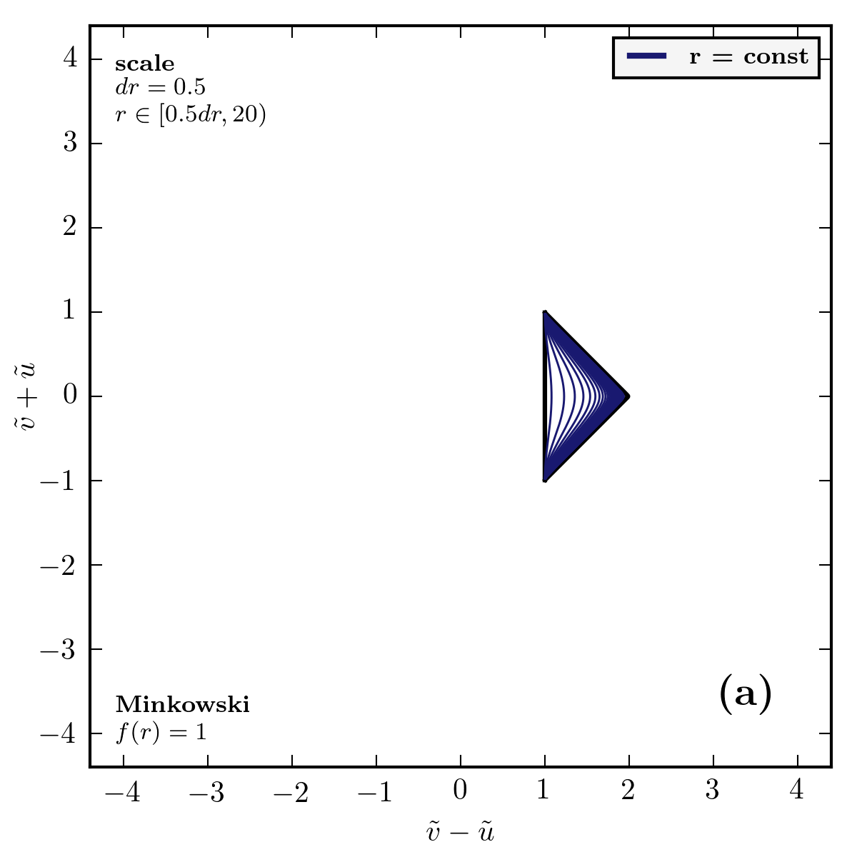
Figure 1 illustrates the basic features of a Penrose diagram in two and four dimensions using the simple case of flat spacetime. In this example, the two-dimensional spacetime is defined by on the coordinate patch and , while the four-dimensional spacetime is defined by on the same coordinate patch. In both cases, the Penrose coordinates are given by and . The resulting metrics are and , where, in four dimensions, the areal radius at each point is given by . Note that the two-dimensional example, which is half of a two-dimensional Minkowski space, is incomplete at by construction so as to more closely parallel the four-dimensional case.
3 A note about units
A detailed review of our unit conventions and their justification is given in B. In short: all coordinates, parameters, tensor components, and lengths appearing in the article are unitless. Proper units are restored by establishing an overall length scale, which can be propagated through all quantities. For details, please see the appendix.
To make the convention as clear as possible, consider the example
| (1) |
The radius , the coordinates , the parameter , the one-forms , and the line element should all be regarded as unitless. To relate this to a physical metric, one would establish an overall length scale . Then the physical coordinates and physical line element would all have units of length, and other quantities would inherit units as appropriate.
4 Strongly spherically symmetric spacetimes and their maximal extensions
The class of spacetimes with metric of the form
| (2) |
(where signifies the metric on a unit -sphere) is of great historical and practical significance: common examples include the Schwarzschild, Reissner-Nordstrom, de Sitter, Anti de Sitter, and Minkowski solutions of GR, among numerous others. Strangely, given their ubiquity, this class of spacetimes lacks a standard name. We introduce some new terminology, and review some properties of these spaces, below.
In particular, we will see that every spacetime which locally has the metric (2) can be isometrically embedded into a spacetime of a larger class, which we will call the “strongly spherically symmetric” (SSS) spacetimes. In this section we develop a detailed geometrical description of such spacetimes.
Historically, our “strongly spherically symmetric” spacetimes have sometimes been called “static spherically symmetric” [11]. But when they are not static (do not have a timelike Killing vector field), so the term is not apt. The new name seems more fitting: the symmetry is “strong” in the sense that, in addition to the spherical symmetries, there exists a Killing vector field normal to the angular directions, which allows the metric components to be expressed as functions of the radius only.
4.1 Spacetimes with spherical symmetry about a fixed origin
To properly describe strong spherical symmetry requires the concept of spherical symmetry about a fixed origin. Since manifolds need not contain their symmetry axes, this requires a little bit of finagling. In C it is shown that for any spherically symmetric spacetime , one can specify the origin of spherical symmetry by selecting a particular algebra of Killing vector fields satisfying certain assumptions. This choice determines spherical orbits of a rotation group; the curvature of these orbits is used to define the radius at each point.
Once the “origin of symmetry” has been fixed by choosing , the areal radius is an intrinsic property of each point , independent of coordinate system. is foliated by spheres (lying tangent to ) with intrinsic metric , except on the axis of symmetry where by definition. Everywhere except on the axis, there is a local coordinate system respecting this foliation, in terms of which the metric is (35).
In our treatment of strong spherical symmetry, we will assume that is spherically symmetric, and that the origin of symmetry has been fixed by selecting a particular . This ensures that local SSS patches all have symmetry about the same origin.
4.2 Coordinate naming conventions
Up to now, our convention has been to denote Penrose coordinates by . Hereafter, Penrose coordinates will usually be denoted by , while coordinates will be reserved for the usual local double-null coordinates with metric (7) below. Coordinates refer of course to standard Schwarzschild-like coordinates with metric (2). And coordinates will denote the Eddington-Finklestein (EF) coordinates with the metric (3) below, such that the EF time may be either advanced or retarded depending on a parameter and a choice of time-orientation. In either case, the vector field is locally equivalent (up to a global normalization) to wherever the latter is defined. For reasons that will become clear below, we will define strong spherical symmetry in terms of the EF coordinate system , and its associated Killing vector field .
At times it is convenient to refer ambiguously to one of the double-null coordinates , without specifying which one. When this is necessary we will utilize the placeholders , where it is understood that either or . The same placeholder convention extends to .
4.3 Spacetimes with strong spherical symmetry
Suppose is a spacetime of dimension , and that is -spherically symmetric with axis fixed by (see section 4.1). Then will be said to have strong spherical symmetry (about axis ) with metric function if every open set has an open subset isometric to222Here and later we abuse terminology by omitting the full statement “isometric to an open subset of on which the metric is defined”, which should be obvious from context. This is equivalent to saying there exists a coordinate patch on in which the metric takes this form.
| (3) |
in coordinates , such that and lies tangent to . Those last bits ensure that all points have a strong spherical symmetry about the same origin. In practice we always define in terms of this metric, so these technicalities become trivial. Assumptions on the function are given below, near the end of this section.
The definition implies that the set
| (4) |
is open and dense in . Using the Eddington-Finkelstein (EF) form (3) of the metric allows to contain points where , and implies that is locally isometric to at points in where .
The spherical symmetry is called “strong” due to the presence of a Killing vector field normal to the angular directions, which allows the metric components to be expressed as functions of the radius only. Indeed, by definition, the metric is independent of coordinate , and so is a local Killing vector field. It is easily seen from the metric that is null wherever , and that is always normal to the angular directions.
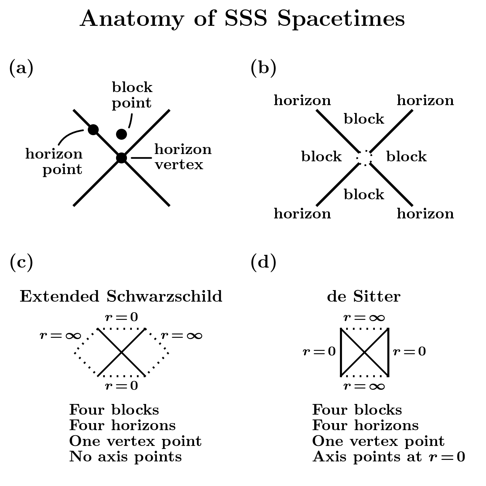
In general, SSS spacetimes can contain four distinct types of points:
-
1.
points not in at which (axis points)
-
2.
points in at which (block points)
-
3.
points in at which (horizon points)
-
4.
points not in at which (horizon vertices)
The reason for these names will become clear later. The isometry associated with flow along preserves this classification, and has the horizon vertices as fixed points. Moreover, every point in has a neighborhood where is an everywhere-nonzero Killing vector field tangent to lines of constant radius. For an illustration of the different types of points, see figure 2.
It is now appropriate to explain the need for fixing the symmetry axis. Without doing so, the presence of additional symmetries can make it impossible to geometrically distinguish points in . Take, for example, the de Sitter spacetime, with metric function . Since de Sitter is homogeneous, every point is geometrically indistinguishable. In particular, every point may be described as lying on a cosmological horizon. From the point of view where we consider de Sitter an SSS spacetime, the additional freedom to choose the origin of symmetry is superfluous (though by no means unimportant). By fixing the origin, we allow points and regions to be classified as above. Additionally, fixing the origin allows us to refer to the radius of a point without reference to any particular system of coordinates.
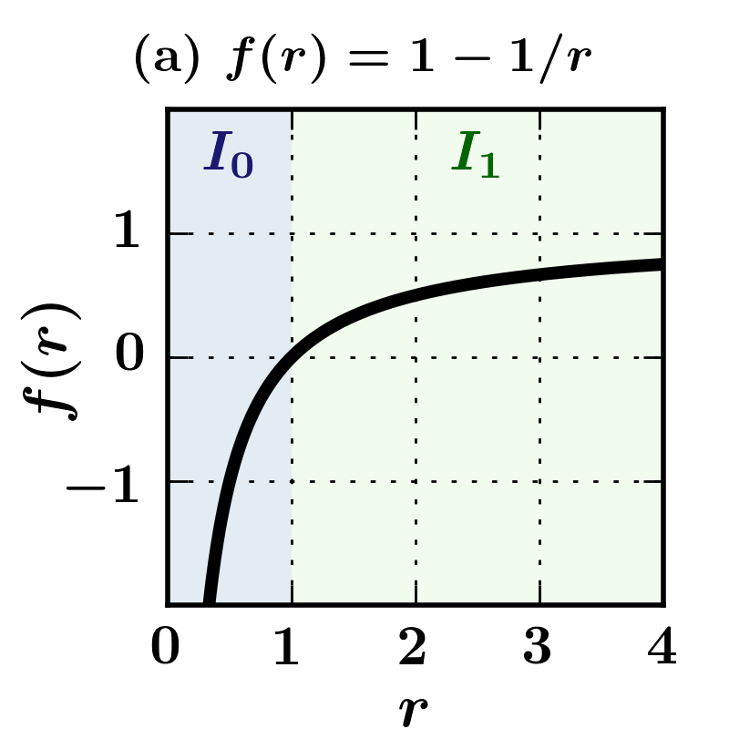
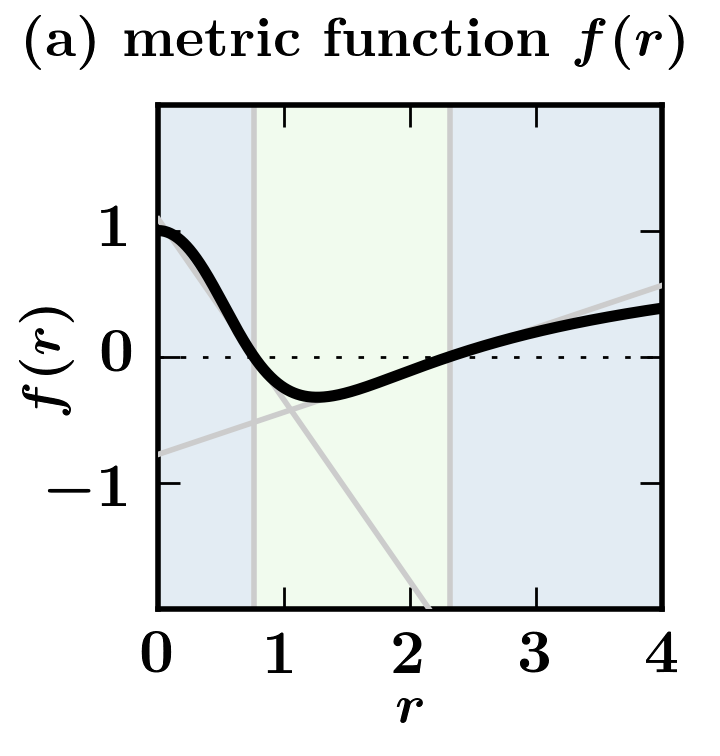
We typically describe a particular strongly spherically symmetric spacetime by specifying its metric function on the interval . For simplicity, we assume that always has the following properties: (I) is continuous and once differentiable; (II) has a finite number of zeroes; (III) is analytic at its zeroes; (IV) all zeroes of are isolated and simple (linear); and (V) .
The assumption that is analytic at its zeroes allows the use of a concise contour integral definition of the tortoise coordinate (see section 5.1); since need not be analytic globally, the assumption is fairly weak. Note that need not be defined. And moreover, the assumption that does not approach zero in the limit is not strictly necessary; it conveniently avoids the treatment of certain edge cases, but can be relaxed with no serious consequences.
It is useful to define a consistent notation for critical values of the radius, in order to partition the radial coordinate into intervals separated by horizon radii. The endpoints of these intervals occur at , at the horizon locations where , and at . We therefore let , denote the zeroes of by for , and let . Then the radius values , for , partition the radial coordinate into intervals , and in each interval the sign of is constant. In this context we reserve the subscript to refer only to the zeroes of , while expressions with subscript additionally include and .
In what follows, a parameter will control coordinate transformations in the vicinity of each critical value of the radius. Near each zero of it must have a particular value, equal to the slope of at , in order for the metric to extend continuously across the corresponding horizon. Where no horizon matching is needed, however, it may be set to zero, yielding a simplified coordinate transformation. In accordance with these requirements, we define at , at the zeroes of , and at . This ensures matching at all horizons, while providing the simplest possible transformations near and , where no matching is needed.
Specifying the metric function determines the local structure of , by insisting that (3) holds for the fixed function . Some ambiguity remains in the global structure. We will see in section 4.6 below that in fact such an might be any subset of a maximally extended corresponding to . This is the class of spacetimes intended by (A) in section 1.
For the remainder of this section, let denote a strongly spherically symmetric spacetime with metric function .
4.4 Horizons and blocks
It is useful to think of as being partitioned into “blocks” separated by “horizons”.
First let us mention the horizons. A connected hypersurface consisting of horizon points in , on which and , is called a horizon. Correspondingly, the values where may be called horizon radii. Every horizon is a null hypersurface, being normal to the (locally) null vector . Moreover, horizons are always Killing horizons, and often trapping horizons (see [12, 13] for definitions). The Killing horizon property is immediate, since the Killing vector field is null at a horizon. The trapping property we will return to shortly. Now let us move on to the blocks.
A block is a region of , consisting of a connected set of block points, which corresponds to a single interval over which the metric function is nonzero. Each block can be covered by the metric (2) defined on a coordinate patch and . Note that this metric may approach a coordinate singularity at the boundaries of the patch. There is a one-to-one correspondence between the intervals and the types of blocks in . However, may contain many blocks of the same type, each corresponding to the same interval . We will often label blocks by their corresponding interval, which indicates their type.
To construct Penrose coordinates for a single block is straightforward. To begin, choose an arbitrary point . Define the tortoise coordinate and tortoise function by
| (5) |
The tortoise function obeys , and is monotonic over since is continuous and nonzero there. Thus is invertible on , and we denote the inverse function by . The arbitrary choice of amounts to an arbitrary additive constant in , which we later absorb into a choice of double null coordinates. The range of depends on the behavior of near the endpoints of ; the value becomes infinite in magnitude near each simple zero of .
Next a set of double null coordinates for the block, with a parameter absorbing the tortoise function’s free additive constant, is defined by
| (6) |
in terms of which the metric becomes
| (7) |
with .
Finally, one chooses two invertible monotonic functions and , called the squishing functions, each with domain and finite range, such that
| (8) |
and such that and are both future directed.
The resulting metric reads
| (9) |
where
| (10) |
and are Penrose coordinates for the block.
Any block bounded by simple zeroes of admits the full range of coordinates and , and therefore covers a diamond in the Penrose diagram. Blocks admitting a smaller range of lie inside this diamond (when the same squishing functions are used).
The freedom involved in obtaining Penrose coordinates according to the above process is less than it may at first seem. First of all, note that the squishing functions should be chosen for simplicity and convenience. Once some squishing functions have been chosen, there is always the possibility to rescale by monotonic increasing functions in the and direction. This basically amounts to a freedom to mess up a nice-looking block, without making any structurally meaningful changes. Therefore let us focus on the choice of . As seen already, the tortoise function implicitly contains an arbitrary constant, which was absorbed into by the free constant . In light of this fact and the freedoms to translate without disturbing the metric, one is tempted to write and . These may be rearranged, however, to yield and . But translations of , being isometries of the block which preserve the range of values (since ), are entirely nonphysical and have no effect on the appearance of Penrose diagrams. The equations (6) are therefore sufficiently general to exhibit all relevant freedoms in the process. Like with the squishing functions, changing the parameter does not cause any important changes to the diagram; it simply alters the appearance, and may be chosen for convenience. Although is free in each block individually, we will see in section 5 that in order to construct global Penrose coordinates for many blocks, the values of in each block must be carefully coordinated, and only a global additive constant remains.
Having now constructed Penrose coordinates for each block, let us use them to investigate the properties of these blocks more deeply.
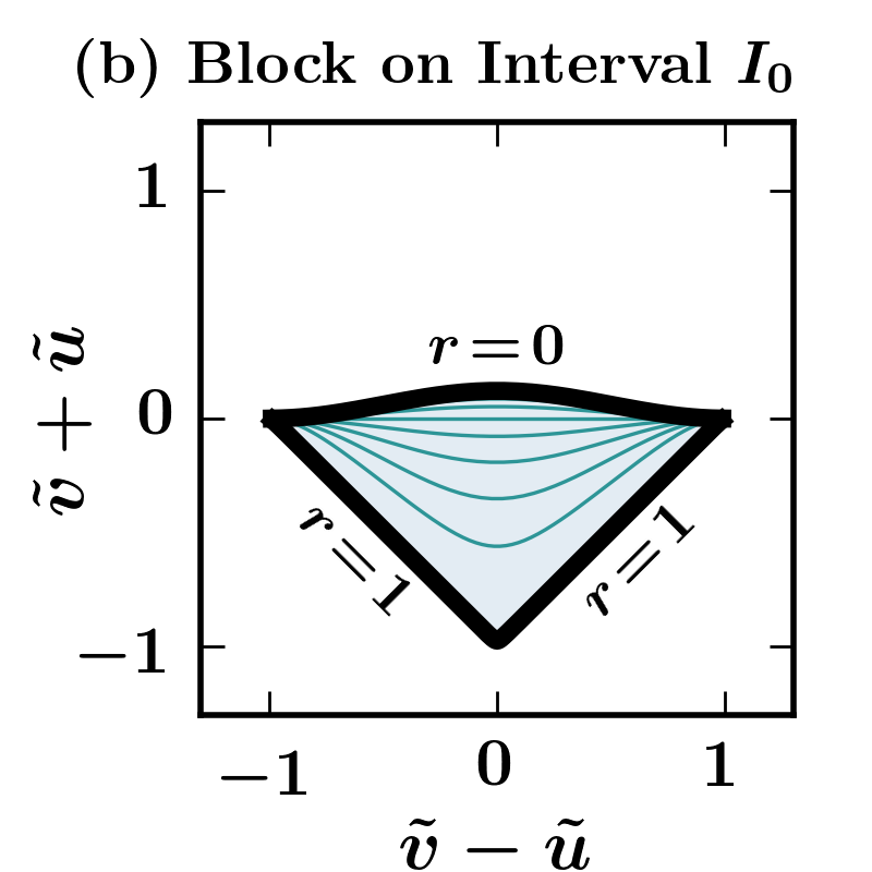
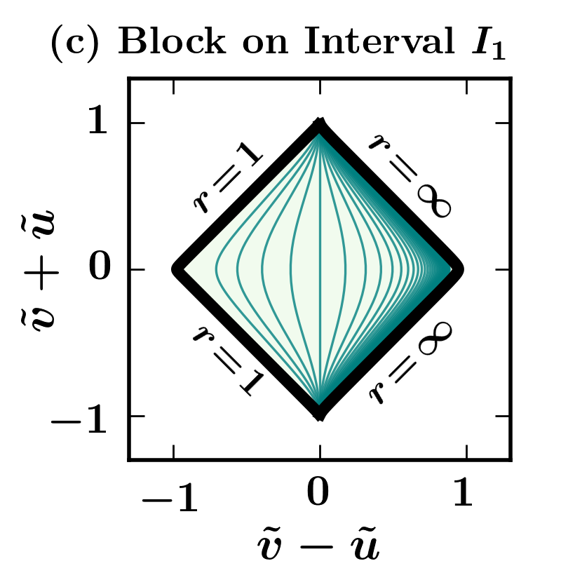
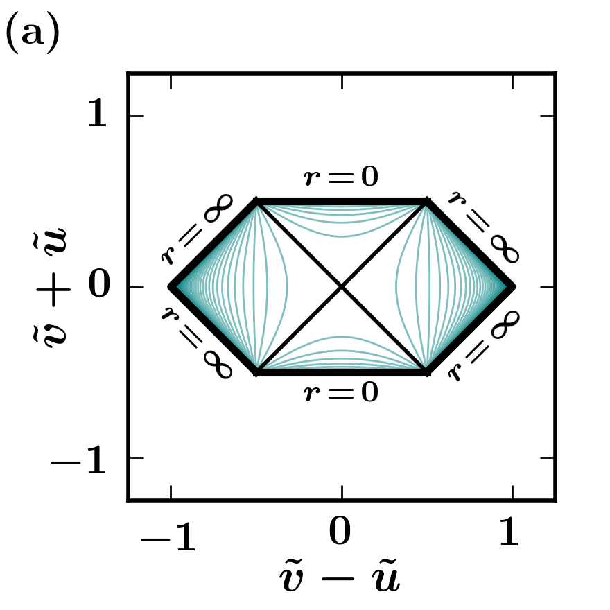
The appearance of a block in the diagram is largely determined by the limits of the function on the interval . In general, each block is bounded by conformal boundaries corresponding to and . When is finite, the block fails to fill its diamond near , and the corresponding boundary is either timelike or spacelike. When is infinite, the block fills a corner of the diamond, and the corresponding conformal boundary is null: it consists of two null horizons joined at a vertex (see figure 4). This makes sense, since whenever is a horizon radius, the line of constant is necessarily null, and the value is necessarily infinite.
As determined by the above-stated dependence on , each block has a causal shape corresponding to its shape in the Penrose diagram. There are three possibilities; we denote them “diamond”, “triangle”, and “slug”. When the conformal boundaries at and both are null, the shape is diamond. When one is null and the other either timelike or spacelike, the shape is triangle. When either both are timelike, or both are spacelike, the shape is slug. All blocks except the first and last necessarily have a diamond shape, and slugs are only possible when has no zeroes. A block’s causal shape is an intrinsic property of the type of block; it is the same in any Penrose diagram of the block, and for all blocks corresponding to the same . Indeed, the tortoise function alone determines causal shape. The orientation of a block in the diagram, however, depends on the sign of in the block, and on the block’s time-orientation.
Every non-slug block, on its own, is extendible (geodesically incomplete without singularity) at its horizons. Indeed, to each horizon radius bounding are associated two classes of incomplete null geodesics: either future-directed and past-directed, or left-going and right-going. These correspond to null rays exiting the two horizons making up the block’s conformal boundary at that radius. It follows that each block bounded by two horizon radii (these are necessarily diamonds) has four such classes of incomplete null geodesics, while each block bounded by one horizon radius (these may be triangles or diamonds) has two such classes. Counting classes of extendible null geodesics suggests how many neighbors a block can have.
We now return to the question of trapping. In E, it is shown that a sphere of constant is a trapped surface if and only if . It follows that within a block with , every point intersects a trapped surface. In light of this fact, blocks on which may sometimes be referred to as trapped blocks, and a union of trapped blocks is a trapped region (more generally, trapped regions are open sets on which every point intersects a trapped surface [14]). Trapped regions are important: an appealingly pragmatic definition of nonsingular black hole is “a future-trapped region terminating in a region of extreme density”. There are various technical notions describing the horizon associated with a trapped region. Suffice it to say that under certain conditions, the boundary of the trapped region can be called a trapping horizon and/or apparent horizon [13].
Figure 3 exhibits Penrose diagrams for some individual blocks of an SSS spacetime with . Note that there remains a freedom to invert the blocks by , since no physical criteria has been given to establish a time-orientation. Parameters for the diagram construction are given in the caption.
Figure 4 illustrates the conformal boundary structure of blocks bounded by two horizon radii.
4.5 Ingoing/outgoing regions, Kruskal quad-blocks, and horizon vertices
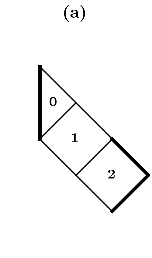
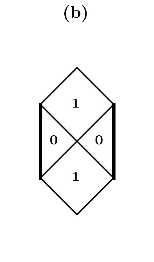
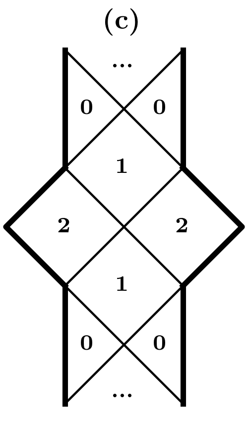
Having observed that is built from blocks, the next step is to see how these blocks can be joined together. There are two useful constructions that make this clear: Eddington-Finklestein (EF) regions, and Kruskal “quad-block” regions. As this section will demonstrate, each of these units highlights an important aspect of how blocks may be joined. In particular, the EF regions show how a chain of blocks can be linked to cover the entire range of radii. Meanwhile, the Kruskal “quad-block” regions show how four blocks can be joined at a horizon radius by four horizons and a vertex. These constructions demonstrate that each block admits either zero, two, or four neighbors. These regions can be visualized using the block diagrams (see section 4.6) of figure 6.
First, we introduce the Eddington-Finklestein regions (figure 6a). A full Eddington-Finklestein region (EF region) is a subset of which has the metric (3) everywhere on a coordinate patch and . Note that there is no coordinate singularity in this patch. When an EF region is time-oriented such that is future (past) directed, it is called an ingoing EF region (outgoing EF region). EF regions are the smallest regions of containing a point at every radius, and thereby are the smallest regions exhibiting the global function . They contain one of each type of block for , with the blocks joined naturally across the horizons. The connectivity of the blocks is exactly the connectivity of the intervals . Nonetheless, EF regions are, in general, extendible.
Every block of can be isometrically embedded into two distinct EF regions, corresponding to the choice in (3), by using the transformation (see section 4.4 for definition of ) to obtain the coordinates from the in (2). The difference between these two regions is that different sets of incomplete null geodesics are extended. These two instances exhaust the block’s extendible null geodesics, indicating that each block naturally has two neighbors for each horizon-radius bounding . Within a given EF region, half of these possible neighbors are realized.
Next we will introduce the Kruskal quad-blocks (figure 6b). The classic example of this structure is the Kruskal diagram for extended Schwarzschild spacetime, with metric function . In this case the Kruskal coordinates are usually constructed by defining using the tortoise function . Exponential transformations are then applied to to attain the Kruskal coordinates, and the resulting metric is shown to be nondegenerate at the horizons. Because this tortoise function is defined analytically, it is easy to miss its key property: that as from both the left and right. This did not have to be the case, as different constants could be added on either side of the discontinuity at without messing up the derivative. This would be quite unnatural to do when is defined analytically, but is perfectly natural when it is defined by a definite integral (e.g. equation (5) above, which would in this case be applied on each side of ). The limit obtained by subtracting out the logarithmic infinity may take any value (a global constant is allowed), but if the left and right limits were different, the metric would be undefined at the horizons.
The issues associated with defining a well-matched tortoise function are described in detail in section 5.1 below. In the present case, it suffices to take a simple generalization of the above observations: to construct a Kruskal quad-block centered at in the general case, a tortoise function must be defined spanning both intervals and , such that , where , for some . This function exists and is unique due to our assumptions (section 4.3) on , and the indeterminate form is analytic at with the limit (see section 5.1). The desired definition may now proceed.
A Kruskal quad-block region is centered on a horizon vertex at where . It contains two types of blocks, corresponding to and , and the tortoise function must be defined as in the preceding paragraph above. A Kruskal quad-block centered at has the metric , in coordinates , where . The metric is defined on a coordinate patch , where the max and min values depend on and . The patch is always nonempty and includes . The point is a horizon vertex; it has no neighborhood isometric to (3) because if it did there would be a smooth everywhere-nonzero vector field tangent to lines of constant radius in that neighborhood. The rest of consists of horizon points at . In case of the traditional Kruskal region with and , one immediately obtains , which is the usual form of the prefactor in the traditional Kruskal metric.
Each quadrant of the Kruskal region is isometric to a single block of . To make this evident, take the transformations and , followed by and , yielding the usual block metric (2). Since every open set in the Kruskal region contains an open patch of an individual quadrant, this also proves that the region has strong spherical symmetry. In these coordinates the action of the Killing vector field looks similar to a boost, and has the vertex as a fixed point. Penrose coordinates for the Kruskal region can be obtained by applying arbitrary squishing functions. Figure 5 shows a Penrose diagram for one Kruskal region.
Having exhibited the EF and Kruskal regions, the possible arrangements of joined blocks should be qualitatively clear. These arrangements are shown in figure 6. Figure 6a and 6b show the EF and Kruskal quad-block building blocks. Figure 6c shows how these can be combined to form larger structures. In figure 6c, each block is a part of two EF regions, and one or two quad-block regions.
4.6 Block diagrams and maximal extension
Since we already know how each individual block looks in a Penrose diagram, and we now know how the blocks can be connected, it makes sense to draw a schematic block diagram of . In such a diagram each block is drawn with the appropriate causal shape and orientation, and connected blocks are drawn sharing the relevant horizon. In this way, the global causal structure and topology of can be accurately presented without need for a global Penrose diagram. Examples of block diagrams are given in figure 6.
Although a block diagram shares the qualitative appearance of its corresponding Penrose diagram, it lacks a global coordinate system. This has no effect on its usefulness as a tool for studying the global causal structure and topology. It does, however, stop us from accurately identifying the lines of constant radius, or plotting scalar functions of spacetime (e.g. the local density or local WEC inequality violation) on the digaram. For detailed analysis of dynamically evolving piecewise-SSS spacetimes, we need these more advanced tools at our disposal.
To wrap up discussion of the global structure of SSS spacetimes, let us introduce the concept of maximal extension. Technically speaking, a (connected) manifold is maximally extended if it can’t be isometrically embedded into a proper subset of another (connected) manifold of the same number of dimensions [5]. In practice, it is often true that a spacetime is maximally extended when all geodesics are either complete or approach a physical singularity. In the context of SSS spacetimes, what we usually mean is that the block diagram for leaves no open horizons. Block diagrams allow maximal extensions of SSS spacetimes to be described pictorially.
For any metric function , there is a maximally extended with the metric function everywhere. The structure of such an an depends on the number of zeroes of the metric function. For every block is already maximally extended on its own. For , the maximal extension is unique and consists of a single quad-block region. For , maximal extensions may have a finite or infinite number of blocks, with a simple periodic structure similar to that seen in figure 6c. A finite number of blocks is possible (but only in the case ) because of a topological ambiguity: torus-like boundary conditions can be allowed so long as closed timelike curves are avoided. Therefore maximal extensions in the case are not always unique, but do always have a unique simply-connected cover. For , maximal extensions are constructed from an infinite chain of quad-block regions, and are not easily represented in a two dimensional block diagram. These necessarily have an infinite number of blocks, and suffer a similar topological ambiguity as the case. When analyzing maximal extensions in the case , it is easiest to represent spacetime by a lattice of horizon vertices, rather than by a set of blocks. However, that method is pursued no further here.
4.7 Boundary points with undefined radius
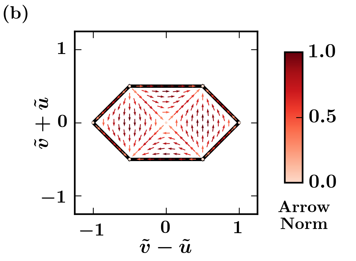
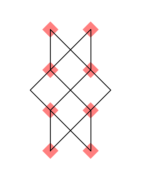
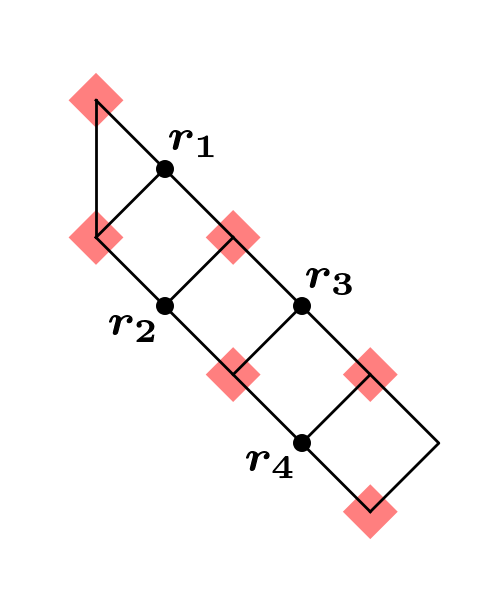
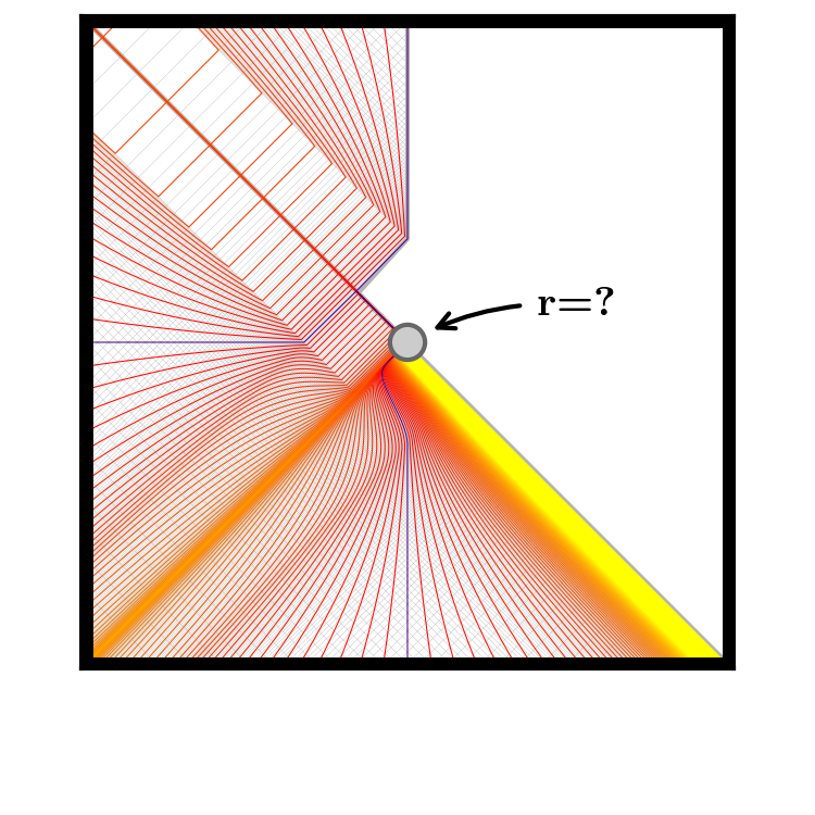
Points where on the conformal boundary of an SSS spacetime have a slight defect: their radius can’t be well defined. This is obvious, since the same boundary point can be approached along lines of constant radius for a continuum of values. For this reason, it is best to think of these points as representing an entire continuum of boundary points, each corresponding to a unique radius. Nonetheless, this continuum is represented in Penrose diagrams by a single point. Figure 7 highlights these defective points in two examples.
The undefined radius points impose a fundamental, but minor, limitation on the possibility of constructing global Penrose coordinates for SSS spacetimes: in any Penrose diagram of an SSS spacetime, each undefined radius point on the conformal boundary has a neighborhood in which the metric may be discontinuous (continuity occurs as a special case but not in general). The affected neighborhoods may be made arbitrarily small by choice of how the diagram is constructed. The red patches in figure 7 are meant to schematically represent the affected neighborhoods.
| (a) | (b) |
|---|---|
 |
 |
Since the neighborhoods where the metric is discontinuous can be made arbitrarily small, the problem imposed by these points is inconsequential. For any subset of , or any worldline contained in , the neighborhoods in which the metric is discontinuous can be “moved far enough out to infinity” so as not to effect the physical problem. In our construction of Penrose coordinates in section 5, a parameter will directly control the size of the affected neighborhoods, such that the neighborhoods become arbitrarily small as .
Fundamentally, the issue is caused by the fact that a single undefined radius point on the conformal boundary may correspond to many different horizon radius values, in many different blocks, at the same time. The technical problem with this may be understood by observing the point between and on the bottom edge of figure 7b. Heuristically speaking, the metric will only be continuous at this point if the same coordinate transformation is applied on both sides. But on either side individually, a transformation must be carefully selected to make the metric continuous at the appropriate horizon (supposing more blocks are added to continue the region through the relevant horizons). Using the same transformation on both sides is, in general, incompatible with choosing the correct transformation on both sides. But since one only needs to be picky about transformations in a small neighborhood of the horizons, the problem can be pushed out into the corner.
The issue of undefined radius points is of a fundamental nature, and is not an artifact of any particular method for constructing diagrams. When there are more than two horizon radii (i.e. zeroes of ), the problem cannot be avoided. On the other hand, in cases where or , there are not enough horizon radii to force a discontinuity in the metric. In the case there are enough horizons to cause a problem, but the discontinuity can be removed by a special choice of transformations. However, the procedure to do so is rather unnatural. Instead, in the method of section 5 we will leave the discontinuities, in order to use more natural transformations, and to keep the treatment unified.
4.8 True Penrose diagrams
We have seen that can be partitioned into blocks, each with a well-defined causal shape. Moreover, we have seen how these blocks can be joined together across horizons in a regular way, and collections of blocks can be represented in a schematic block diagram. Lacking, so far, is a method for joining an arbitrary number of blocks, explicitly, in double-null coordinates.
This goal can be achieved in two key steps:
-
1.
taking a global contour integral definition of the tortoise function; and
-
2.
using a particular form of the squishing functions for each block.
Applying these steps results immediately in Penrose coordinates for , in which the metric extends continuously and nondegenerately across all horizons. This will be the subject of section 5.
5 Explicitly computing Penrose diagrams for SSS spacetimes
This section provides the recipe for explicitly constructing Penrose coordinates for SSS spacetimes. First, a global tortoise function is defined using a contour integral. Then a useful choice of the squishing function for each block is defined. Finally, the algorithm for generating Penrose coordinates is stated in full, and the resulting metric is shown to be nondegenerate.
We continue to assume that satisfies the criteria laid out at the end of section 4.3. In particular has simple zeroes at (for ) such that , and is analytic at each of its zeroes. We denote and , and the intervals are defined for . The parameters are defined by where no matching is needed, and by at the horizons.
5.1 Global tortoise function
A tortoise function is by definition an antiderivative of . This leaves an arbitrary integration constant in each block. These must be coordinated such that, when the logarithmic infinities at the zeroes of are subtracted out, what remains is continuous. We adopt a definition for such a global function which is both analytically useful and numerically approximable. The only free parameter in this definition is a global additive constant, which has been absorbed into the definitions of .
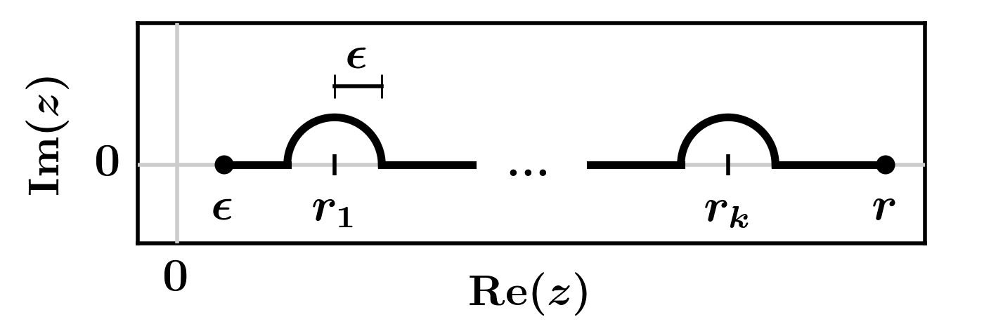
Let denote a contour in the complex plane which begins at , ends at , and follows the real axis except for avoiding zeroes of using semicircles of radius in the upper half plane. Since is assumed analytic at its zeroes, is well-defined on the contour for sufficiently small . This contour is depicted in figure 8.
The global tortoise coordinate and global tortoise function are defined by
| (11) |
Clearly this definition obeys the defining relation . Within each interval the tortoise function is monotonic and invertible, and we denote the inverse functions by . The semi-circular contours each contribute the purely imaginary value in the small limit. Thus for sufficiently small .
It follows from the above considerations that (11) is approximated by
| (12) |
| (13) |
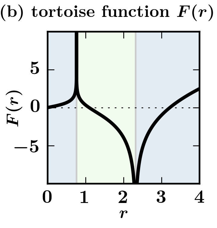
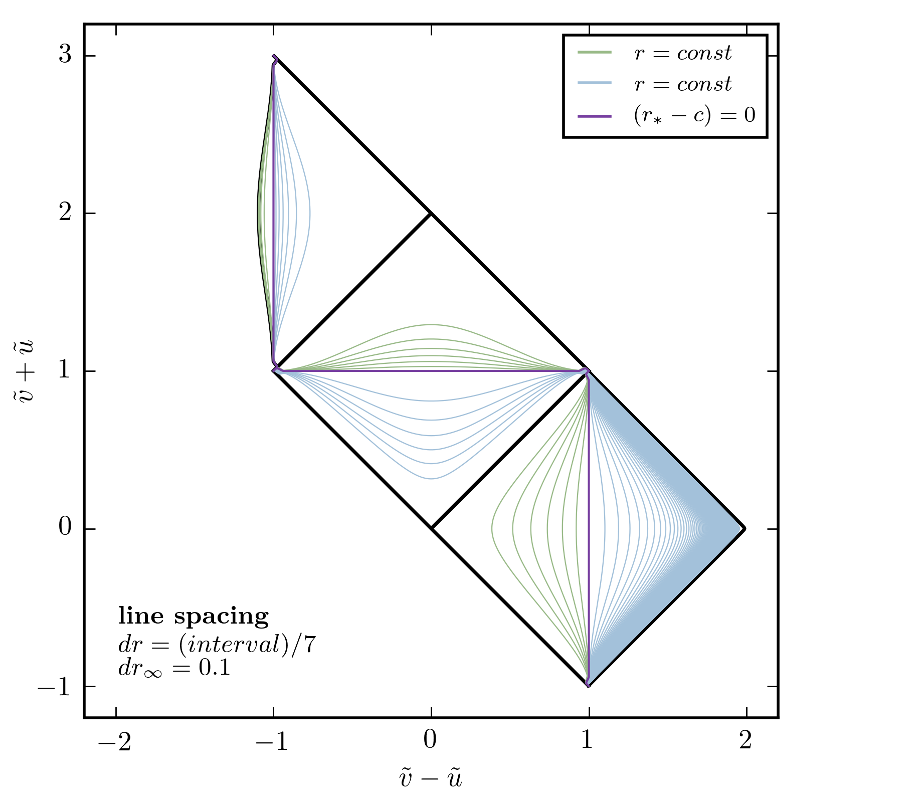
with a small parameter . This form can be computed on a dense spacing of points by numerical integration. The forward and inverse functions can then both be approximated by linear interpolation. For improved numerical precision, it may be best to implement these formulae by integrating from some less extremal point in the interval, and matching boundary terms with additive constants. An example of the global tortoise function thus defined is given in figure 9.
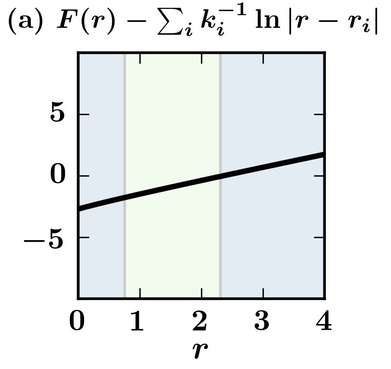
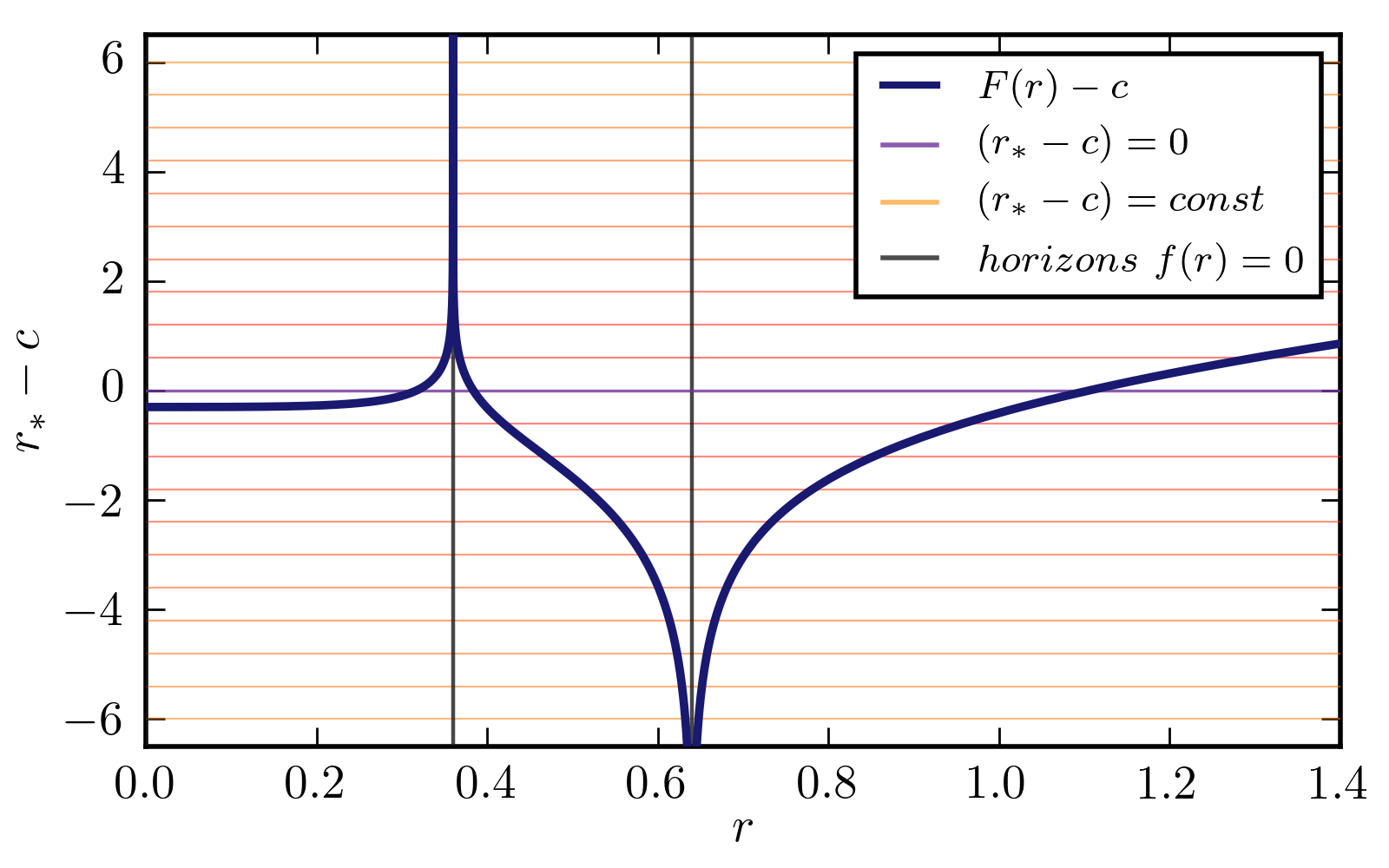
By assumption, is analytic and linear at each of its zeroes. This fact, in tandem with the definition (11), gives the global tortoise function two key properties. Most importantly, the expression
| (14) |
is analytic and strictly positive in a neighborhood of . This fact is essential for establishing that the metric is nondegenerate and continuous at the horizons; we will find that (14) appears explicitly in the Penrose coordinate metric (23). And secondly, the expression
| (15) |
is analytic in a neighborhood of . This result is of mainly conceptual importance, and relates closely to the first. These two properties can be understood by simple heuristic arguments in the real domain, and are also proved more rigorously in D; they are demonstrated by example in figure 10.
Having defined the global tortoise function and determined its properties, the transformation to global Penrose coordinates can be undertaken.
5.2 Double-null and Penrose coordinates
The global tortoise function makes it possible to define Penrose coordinates in which the metric is non-degenerate at the horizons. But to do so still requires that the coordinates be defined just right.
The approach given here differs in philosophy from the more well-known Kruskal method. There, the blocks are joined first and then all jointly squished. Here, instead, each block is squished individually, and the squished blocks are placed next to each other. This type of technique was pioneered by Carter [3]. The transformation in each block relies on an exquisite balance between arctangent compression and exponential expansion; when done right, a seemingly miraculous cancellation at the block boundaries renders the metric continuous.
First, the transformation to double-null block coordinates proceeds in the standard way, utilizing the global tortoise function. In particular,
| (16) |
The global parameter absorbs the global integration constant left in the tortoise function, and must be the same in every block. For the same reasons explained in section 4.4, the definition of should have only the parameter , and cannot be made more general by including other parameters.
The transformation from block to Penrose coordinates is then defined by
| (17) |
The constants and locate the center of the block. The constants and determine the block’s orientation, and must obey
| (18) |
The function must be chosen carefully in each block, and is defined below. For notational purposes, will be written as , with a generic argument of no physical significance. The function is referred to as the pre-squishing function, since it is applied to block coordinates before arctangent squishing functions are applied.
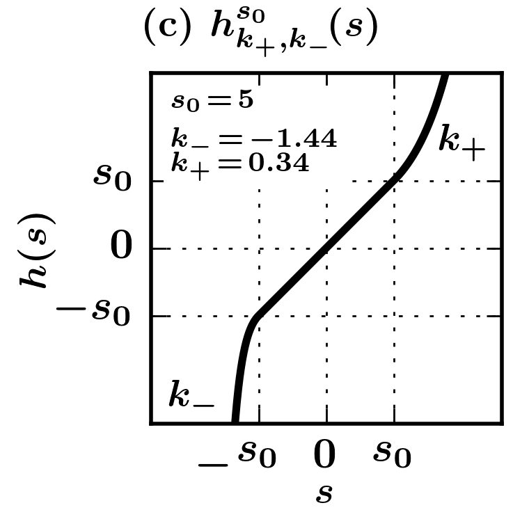
All that remains is to define the function in each block. There is some amount of freedom in this definition, as discussed in more detail below. We take the definition
| (19) |
where
| (20) |
with a parameter of the diagram construction, and with and parameters determined by the metric function in the block. In particular, for a block on radius interval , the parameters are
| (21) |
where at and , and at horizons (see second half of section 4.3). Since by this prescription , it is always true that is continuous, differentiable, monotonic increasing, and unbounded as . Figure 9c shows an example of for a particular block.
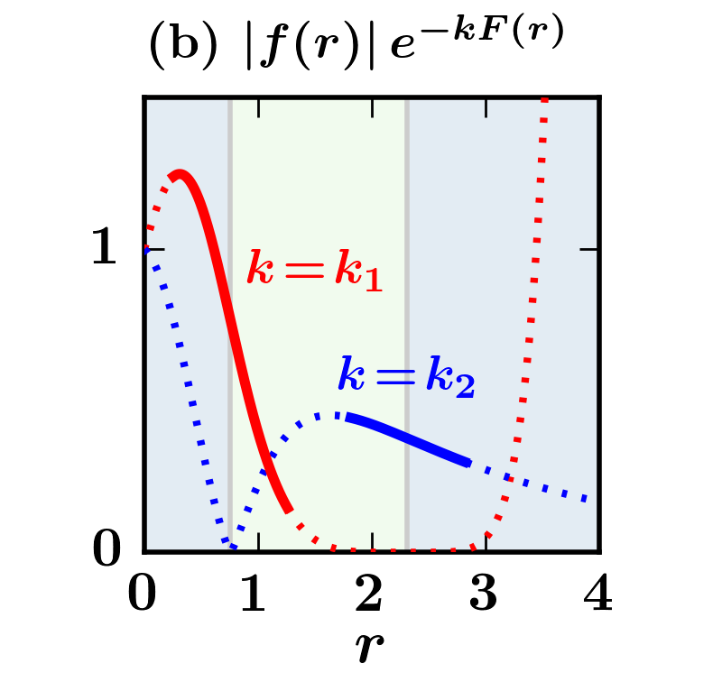
The parameters control the exponential behavior at the tails of . This behavior is essential to obtaining a continuous metric at the horizons. The setup is such that near each horizon radius , the corresponding slope controls the exponential transformation. Near and there is no need to match the metric; recalling that, by definition, at and at (end of section 4.3), one can see that remains linear at these locations. Although the definitions ensure that is everywhere continuous and once-differentiable, large values of cause a rapid exponential turn-on that appears similar to (but is not) a kink in the first derivative.
Whereas control the form of the exponential regions of , the parameter controls the location of the exponential regions in the diagram. As , the exponential turn-ons are pushed arbitrarily far up against the horizons and into the corners of the diagram. As discussed in section 4.7, as there must always be a neighborhood where the metric may be mismatched. The parameter controls the size of these neighborhoods: the metric is never discontinuous unless both and . We typically choose such that the exponential regions are visible but not overwhelming in the diagram.
There is some amount of freedom to choose an . Only the monotonicity and asymptotic behavior at are absolutely essential. But choosing the function poorly can lead to difficult calculations and very ugly diagrams. The choice above is based on several additional criteria: (i) the function is continuous and once differentiable; (ii) lines of constant radius in the resulting diagram look natural; (iii) the function has a closed-form inverse; (iv) metric calculations are relatively simple; and (v) issues near the points are minimized.
Thus have the Penrose coordinates been constructed. The resulting metric is given in section 5.4. It remains only to show how the blocks should be matched up such that the Penrose metric is continuous and non-degenerate at horizons.
5.3 Joining blocks in Penrose coordinates
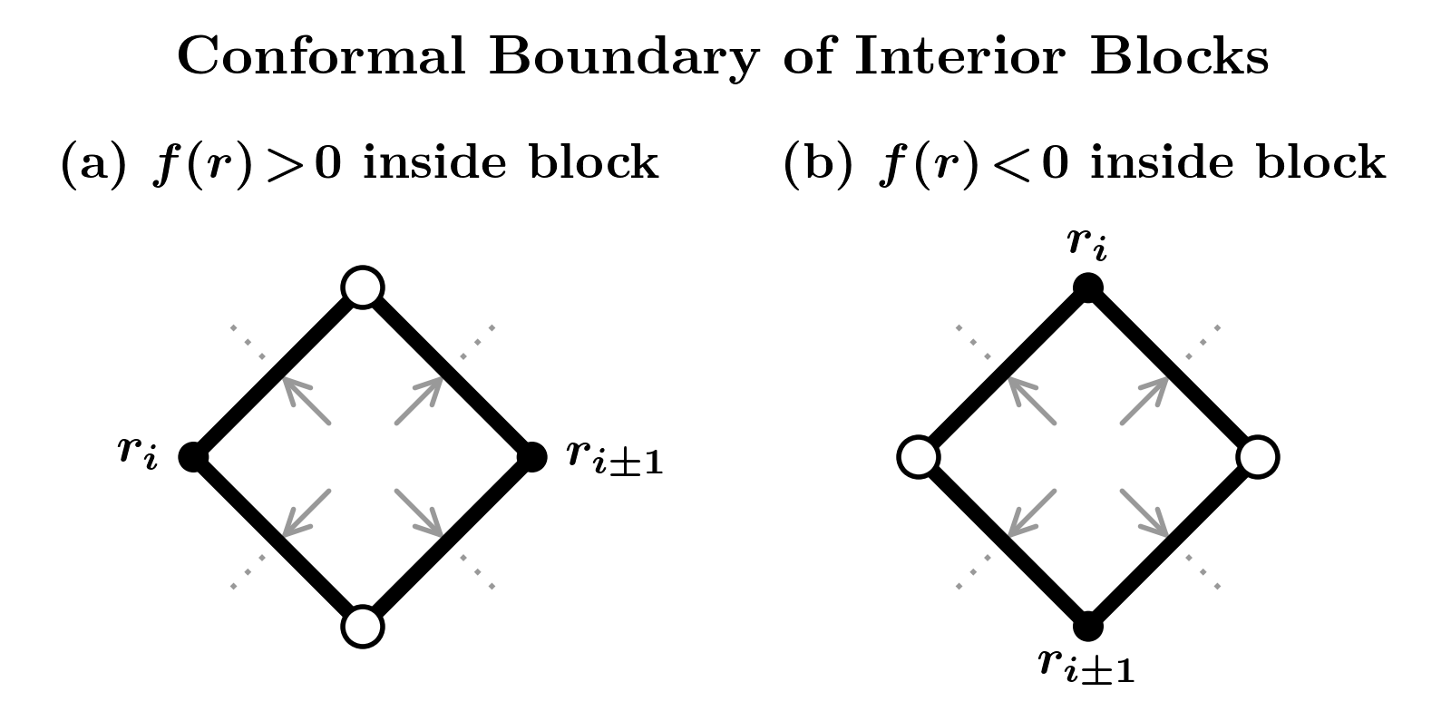
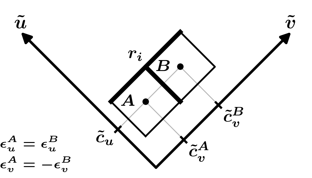
Two blocks can be joined along a horizon at if and only if the two blocks correspond to and . Let two such blocks be denoted and , respectively. The necessary parameter constraints for matching are determined by simple considerations. The setup is depicted in figure 11.
In order that the blocks be squarely aligned, it is necessary that either or . For the horizons to intersect, the pair which is not equal must obey (where represents either or ). We can therefore say that the blocks are shifted in the coordinate , and aligned in the other coordinate . The matched horizon then traces out a line of constant in the diagram. In order that the orientation of this horizon be preserved, it is necessary that . But since the metric function switches sign in subsequent intervals, one obtains the further requirement . This implies that along the shifted coordinate. The only remaining parameter freedom is the sign of the above translation. In order to avoid introducing a time-orientation, this can be handled by simply stating that the matched horizons must be at an equal radius. This condition can be easily checked.
These requirements may be summarized as follows. Let and be blocks corresponding to and . The two blocks may be joined either along a line of constant , or along a line of constant . In order to treat both cases simultaneously, fix the symbols to mean either or (see section 4.2). The blocks will be joined along a line of constant . Then the blocks are properly matched at if:
-
(i)
and ;
-
(ii)
;
-
(iii)
;
-
(iv)
both intersecting horizons have the same radius .
For a fixed orientation of , this yields exactly two ways to attach , corresponding to the choice of . In D, it will be shown that these conditions suffice to ensure non-degeneracy of the metric.
5.4 Enumeration of the algorithm
All the ingredients are in place. In this section, we concisely summarize and enumerate the algorithm that has been presented for generating global Penrose coordinates for an SSS spacetime with metric function .
Suppose is an SSS spacetime with metric locally of the form
| (22) |
Assume the metric function is once-differentiable, has a finite number of zeroes on the interval , and that . Further, assume that is analytic at each of its zeroes, although it may not be analytic globally, and that each zero is isolated and simple (linear).
The zeroes of are denoted for , and at each zero there is a slope . Additionally, denote and , along with . Then the radius values , for , partition the radial coordinate into intervals , and in each interval the sign of is constant. Note that unlike at the zeroes of , the values and do not correspond to slopes, but are zero by fiat. This is because at and , no horizon matching is needed.
First one must choose several global parameters associated with choices in the diagram construction. These control the appearance of the diagram. Additionally, the tortoise function , which determines the transformation into double null coordinates, must be defined globally in the correct way.
-
(i)
Choose the global parameters and .
- (ii)
The parameter absorbs an integration constant in the tortoise function and acts as a translation in the double null block coordinates. The parameter determines the location of exponential turn-ons in the piecewise function below. Increasing pushes certain details into the corners of each block.
A block is specified by its interval . For each block in the diagram, appropriate block parameters must be chosen for the transformation to Penrose coordinates. For each block:
-
(iii)
Let .
Let .
(Recall that for and ). -
(iv)
Choose block parameters and .
Ensure these are chosen such that .
These control the location and orientation of a block.
Having set the parameters in each block, the transformation to double null coordinates , then to Penrose coordinates , can be defined. For each block:
-
(v)
Let as defined by (19).
-
(vi)
Let .
Let . -
(vii)
Let .
Let .
The coordinates are now Penrose coordinates for each block by the definition of section 2. In order to ensure that the Penrose coordinates are global, parameters in each block must be compared.
-
(viii)
Check that all adjacent blocks are properly matched according to the criteria listed at the end of section 5.3.
These conditions ensure that all blocks overlap only on the appropriate horizons, and that relative block orientations are correct.
The resulting metric in Penrose coordinates is implicitly defined in terms of and by
| (23) |
where we have introduced a free parameter , and
| (24) |
| (25) |
The areal radius is given in each block by
| (26) |
The metric (23) is independent of the free parameter , which cancels out entirely when and are substituted back into the metric. Thus (23) holds for every . The purpose of introducing artificial dependence on is to make it easy to evaluate limits at each by setting . This trick works on both sides of every (i.e. approaching from blocks on or ), due to the piecewise definition of in each block. Note that with the appropriate substitution for , the explicit function of radius appearing in the metric is equivalent to (14).
In the above form, all metric coefficients of and of are explicitly non-negative everywhere, and explicitly positive at all block points. In can be shown that these coefficients are also positive at horizon and horizon vertex points. In D it is shown that this metric is continuous and nonzero everywhere, except along the polar coordinate singularity at , and except possibly in arbitrarily small corners of the diagram where , , and (as discussed in section 4.7). Thus, the metric extends continuously and without degeneracy across all horizons and horizon vertices.
This form of the metric depends upon the Penrose coordinates only implicitly, through its dependence on and . This leaves the freedom to translate and flip blocks in the Penrose coordinates without a meaningful disturbance of the metric. Once the diagram is set and the blocks are matched, arbitrary monotonic functions and can be applied without compromising the Penrose coordinates; this usually just makes the diagram look worse, but is necessary in section 6.
6 Extension to piecewise-SSS spacetimes with null-shell junctions
In the astrophysical universe, spacetime is not strongly spherically symmetric – it is constantly, dynamically, evolving. Fortunately, many dynamical phenomena can be approximately modeled by spacetimes which are piecewise-SSS. Basic examples include stellar radiation, stellar collapse to a black hole, and the emission of Hawking radiation from a black hole.
The class of spacetimes treated in this section, which we refer to as piecewise-SSS spacetimes with null-shell junctions, is defined by having a finite number of SSS components, each joined together along null junction hypersurfaces. The junction hypersurfaces correspond to thin null shells of matter. These junctions may have either the geometry of a single null shell (figure 13b), or of two null shells colliding at a corner (figure 13a). The full metric and other tensors are defined distributionally on the piecewise spacetime.
In this section we state the procedure necessary to construct piecewise-SSS spacetimes, making use of the Penrose coordinates previously identified. This immediately yields Penrose coordinates for the piecewise spacetime. First, we present the procedure for shell and corner junctions under the minimal requirement that junction shells have well-defined intrinsic geometry. Then, we determine the matter content of junction shells and discuss the conservation of energy.
This section is largely informed by the classic exposition of Barrabès and Israel [15], which is the standard reference for the analysis of thin shells and piecewise-defined spacetimes.
6.1 Geometry of a radial null slice in SSS spacetime
Consider an EF patch of an SSS spacetime, covered by the coordinates and metric (3). As usual, is the parameter appearing in the EF metric. Assume, without loss of generality, that is future-directed. (This is general because with is an isometry of the EF patch.) With this convention, it follows that
| (27) | |||
| (28) |
and that is always future-directed. This convention applies throughout section 6.
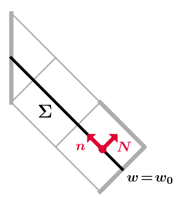
With this setup, a radial null slice of the patch is defined as a hypersurface of constant , as depicted in figure 12. Such a hypersurface is parameterized by the coordinates , and obtains the induced metric
| (29) |
in the coordinate basis.
A normal vector and transverse null vector to can be defined (in the abstract index notation for spacetime tensors) by
| (30) |
such that and . Note that and are both future-directed. As usual for a null hypersurface, the normal vector is tangent to , and is a degenerate vector of in the induced metric. This implies, as usual, that has a geometrical dimension one less than its topological dimension .
Before moving on, it worth noting that the normal and transverse vectors to are eigenvectors of the stress tensor on the EF patch. At block points in the patch, the stress tensor is given in an ortho-normalized Schwarzschild coordinate basis by (62) of the appendix. This stress tensor has two degenerate eigenspaces. Using this fact, one can note without calculation that, at block points,
| (31) |
since both and lie entirely in the plane. Direct calculation in the EF coordinates reveals that these same eigenvalue relations hold also at horizon points, and thus everywhere throughout the EF patch.
6.2 Algorithm for implementing corner and shell junctions
Four SSS (or piecewise-SSS) spacetimes can be joined together at a corner, which represents a pair of colliding null shells. The basic restriction for such a junction is that every point have a well-defined radius, so that the induced metric on the junction hypersurfaces is well-defined. Here we present a method for attaining a junction under this minimal condition. Later, more detailed conditions for energy conservation are given. For the sake of simplicity, in this treatment the corner junction point is always located at a block point. Although it is possible to locate the corner junction at a horizon or vertex point, to do so requires a separate treatment. Keep in mind that, despite the similarity in their schematic illustrations, a corner junction point is not the same thing as a horizon vertex. Once the algorithm for corner junctions is established, the procedure for shell junctions follows as a special case.
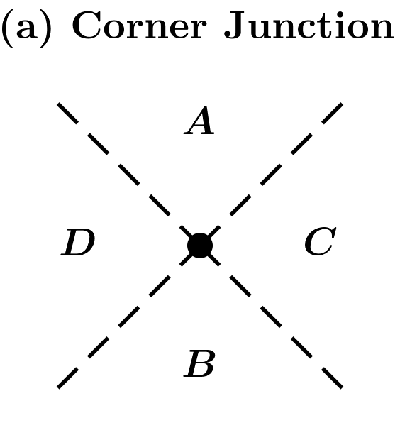

Consider four SSS (or piecewise-SSS) regions, labelled , and called the input regions, to be combined into a piecewise unit. Let each input region have Penrose coordinates . The input regions will be mapped into a target space representing the joint spacetime, as in figure 13. The coordinates of the target space we call . For each input region, the transformations and into the target space must be specified.
The procedure by which the input regions are joined can be stated simply: each input region must be sliced along null junction surfaces in the and directions, then stretched and shifted in the and directions such that the radii at junction surfaces are all matched up. This procedure is illustrated schematically in figure 13c. A precise formulation of the procedure is as follows.
First, one must choose null slices in each input region to act as the junction hypersurfaces. This amounts to choosing values and in each (the values in each region may be distinct). Junction slices are then located at and , with the corner point located at the intersection . The values must be chosen consistently, such that the corner points for each input region have the same radius . We call this shared radius the corner radius.
With the junction hypersurfaces consistently defined in the input regions, one is free to define an arbitrary radial parameterization of the junction hypersurfaces in target coordinates. This is done by specifying two arbitrary monotonic functions and . Each input region will be mapped into the target region so that the radii match these functions on the junction surfaces. The corner point will therefore attain the coordinates in target coordinates.
Having achieved this setup, the transformation of each input region into target space coordinates is given by
| (32) |
When junction slices cover less than the entire domain of values, the above transformations may be extended by an arbitrary monotonic extrapolation. The transformations ensure that the radii and are well-defined regardless of the region of evaluation. Moreover, a simple chain rule calculation leveraging the results of sections 5.1 and 5.2 reveals that when the input regions are SSS, the junction slice radii and are monotonic functions. This implies that whenever and are monotonic, the target-space metric components for each input region are regular and nonzero. This ensures that the transformations (32) will yield Penrose coordinates for the joint spacetime. Furthermore, it follows from the chain rule that and are monotonic functions in the target coordinates. Thus even when the input regions are themselves piecewise-SSS, the above procedure yields Penrose coordinates in the target space.
The full metric of the joint spacetime is defined piecewise in terms of the input region target-space metrics; it can be written distributionally using Heaviside -functions. The arrangement is depicted in figure 13a. With this setup, the induced metric on the junction hypersurfaces is . Since the radii at these hypersurfaces has been properly matched, the geometry of the joint spacetime is well-defined and non-degenerate. The coordinates are Penrose coordinates, and our theory of corner junctions is complete.
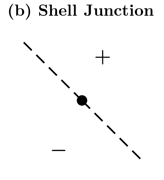
A shell junction can be regarded as a special case of the corner junction, in which two pairs of the input spacetimes are identical. In such a case, all the above considerations remain valid. Additionally, for a shell, radius matching in either the or direction becomes trivial (depending on the direction of the shell), so that one of the transformations in (32) can be replaced by or , or some other monotonic function, if desired.
This procedure achieves our goal of constructing a composite spacetime under the minimal junction condition.
6.3 Matter content at shell junctions
In order to analyze the matter content at a shell junction generated by the above algorithm, it is easiest to work in local EF coordinates of the type set up in section 6.1, rather than in the Penrose coordinates of the previous section. Suppose we focus on a local patch , which is separated into a past region and future region by the null junction hypersurface , with the metric functions in the two regions. Each of can be expressed in terms of EF coordinates, with metric of the form (3), such that lies on a line of in each region, and such that . It is therefore possible to choose a joint coordinate system on , such that is defined by the level set , and such that the metric is (3) with metric function in the appropriate regions. In accordance with section 6.1 and the requirements of [15], the metric parameter indicates the future-/past- directedness of , the normal and transverse vectors and are future-directed, and the level set function increases toward the future.
In order to conveniently express the stress tensor, let us define the mass function by , and define the mass jump . Note that no restriction on is implied — it is simply a useful way to write the metric function. Then, in the joint EF coordinate system described above, the stress tensor associated with the junction shell may be read off from [15, (s. II, IV)]. In the abstract index notation for spacetime tensors (as opposed to the notation convention of [15], which uses latin indices for hypersurface coordinates), it reads
| (33) |
where is both normal and tangent to the shell, the metric parameter indicates an outgoing () or ingoing () shell (see sec 6.1), and is the Dirac -distribution.
The coefficient may be thought of as the surface energy density of the shell, up to an arbitrary normalization factor associated with the null vector . A more physical quantity is the surface energy density relative to an observer with future-directed timelike tangent vector , which is given by . Evidently the sign of is physically meaningful: timelike observers measure a positive energy density if and only if . Indeed, one can show that when the null, weak, and dominant energy conditions are violated, and the energy flux vector (relative to a future-directed timelike observer) is past-directed null. It is therefore sensible to say that shells with have negative mass, while shells with have positive mass. The sign of is a local property, and in principle (in physically unusual cases) a single shell may have positive and negative mass at different points.
Schwarzschild Junction: Positive Mass Shell Scenarios
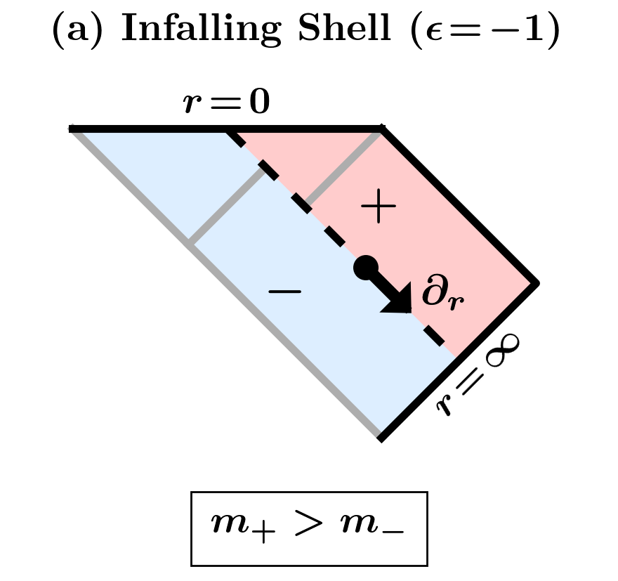
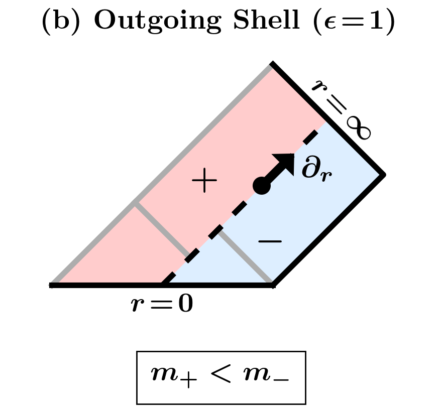
For the junction of two patches of Schwarzschild spacetime, the mass jump is a constant value ; the positive mass shell scenarios () for this case are depicted schematically in figure 14. If the inequalities in the figure were reversed, the junction would yield a shell with negative mass.
6.4 Energy conservation at shell and corner junctions
Local conservation of energy and momentum in General Relativity is expressed by the relation . For any smooth metric, the contracted Bianchi identities provide , ensuring energy conservation by way of Einstein’s equation. When the metric is not differentiable, the standard derivation of the Bianchi identities does not hold up. So the question remains: for the piecewise case, does local energy conservation hold everywhere as a distributional identity?
For the case of shell junctions, it has been shown by Barrabès and Israel [15, (eqns. A10 - A13)] that does indeed hold as a distributional identity. It is therefore true that, without any further constraints, the joint spacetime produced by our junction algorithm is automatically energy conserving at all shell junctions. In context of our junction algorithm, every junction is locally a shell junction except at the corner points in the target coordinates. So the only remaining question is that of energy conservation at the corner points.
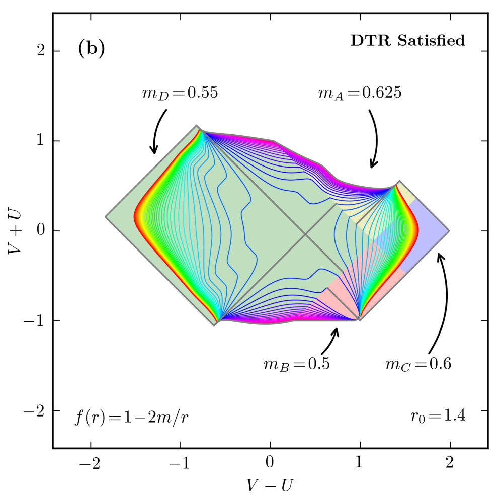
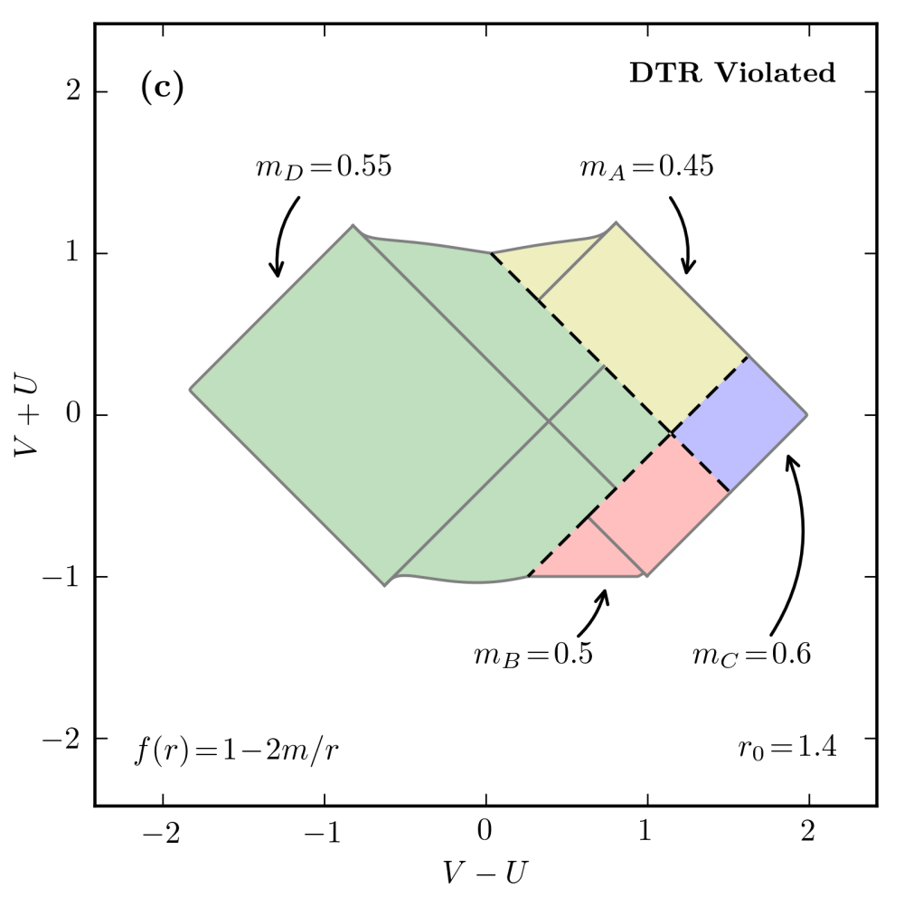
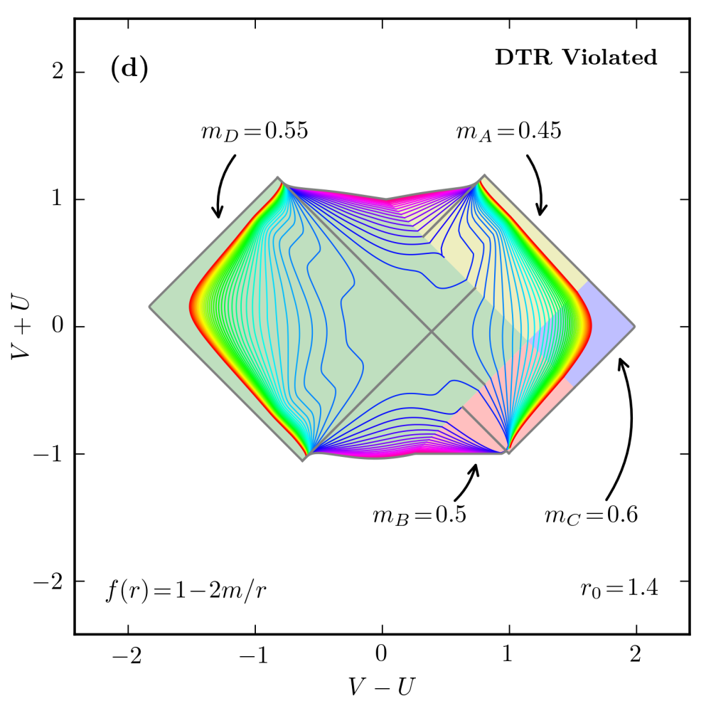
At corner points, the question of energy conservation is slightly more complicated, but there is nonetheless a well-established theory [15, 16, 17, 18]. In order that conservation hold at a corner point with radius , the metric functions of the four input regions must satisfy the DTR (Dray - ’t Hooft - Redmount) relation [18]
| (34) |
with the region labels defined by figure 13a. This formula encodes a relativistic version of conservation of mass in the shell collision. Note that when shell junctions are regarded as a special case of corner junctions, the DTR relation is satisfied trivially. It is well known that the DTR relation is necessary for energy to be conserved, and general consensus of the standard treatments of shell collision (cited above) suggests that the relation is also sufficient. However, the authors are not aware of an explicit proof that the distributional equation holds at corner points when DTR is satisfied.
7 Implementation and examples
The methods described in this article have been implemented in a package called xhorizon for Python 2.7. Source code for the implementation is available from the authors.
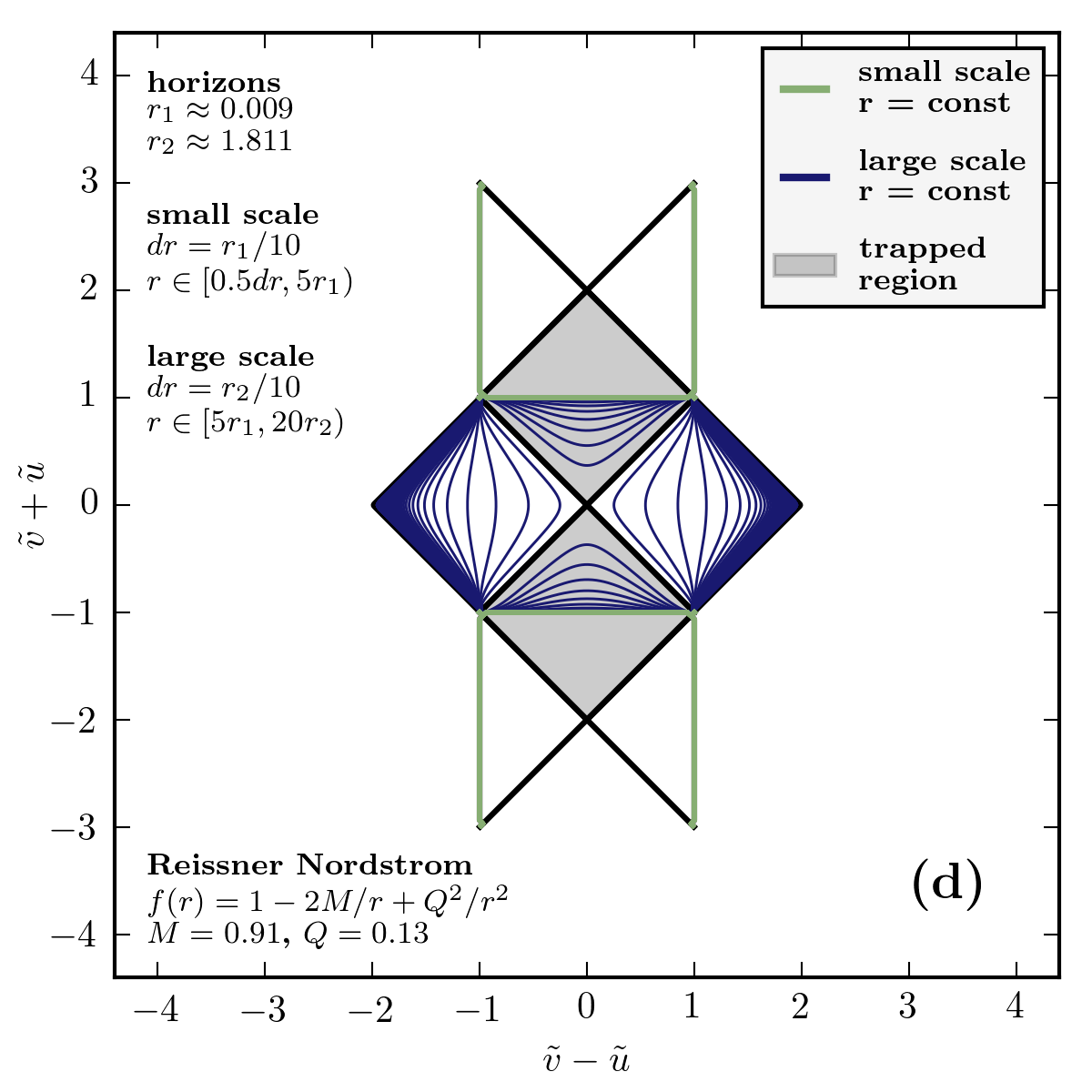
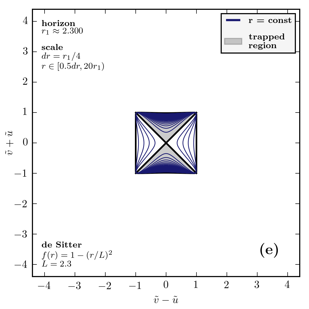
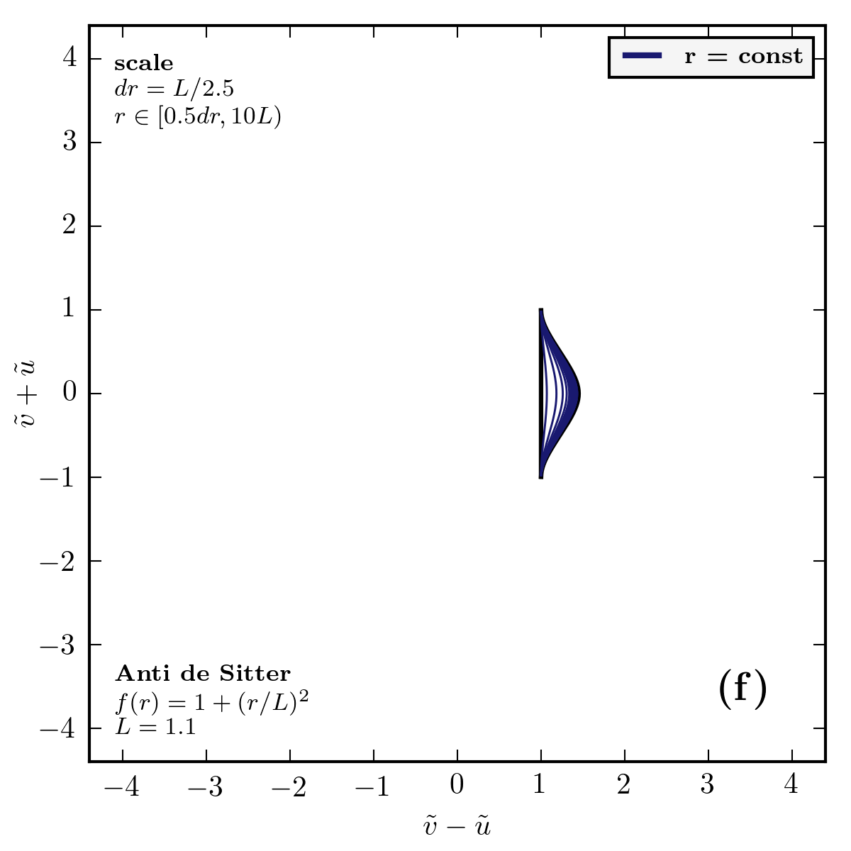
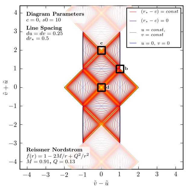
Examples generated by the implementation are given in figures 15–18 (located after the end of the text but before the appendix). Figure 15 depicts example diagrams for SSS spacetimes. Figure 16 shows a detailed zoom view of a particular diagram. Figure 17 helps elucidate generic features of the diagrams resulting from these methods. And figure 18 gives example diagrams for piecewise-SSS spacetimes resulting from null shell junctions.
Features of the examples and implementation are described in captions of the example figures, since they are best understood in context of the results. Just a few further comments are in order here.
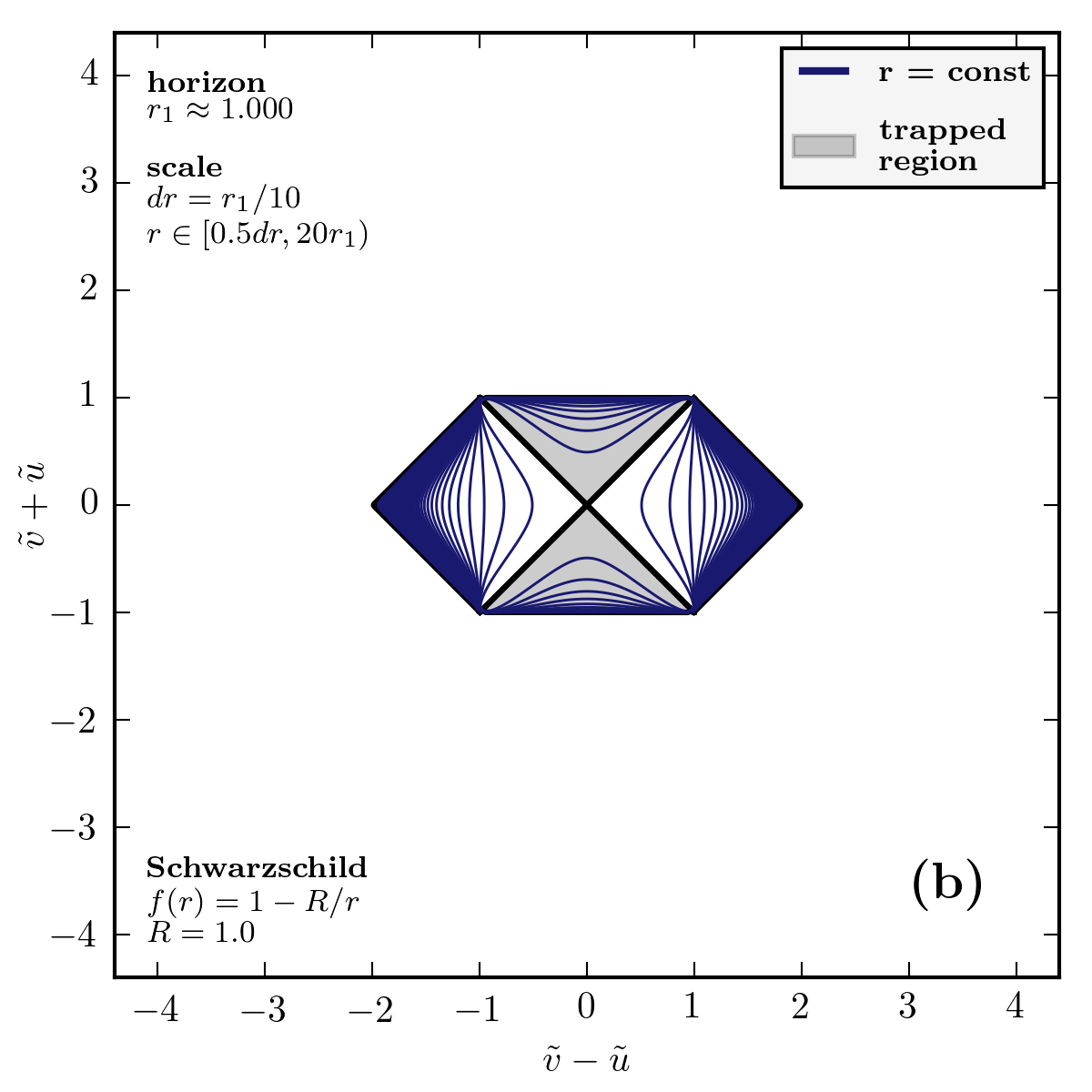
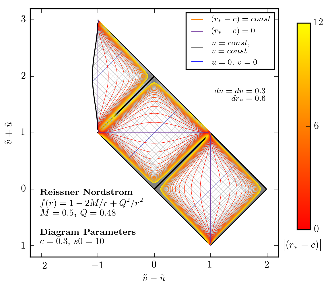
The first comment regards the SSS diagrams. Comparison between the extended Schwarzschild diagram in figure 15b and the Reissner-Nordstrom (R-N) diagram in figure 15d is immediately striking: for all lines of constant radius on the length scale of the outer horizon radius, the two diagrams are nearly identical. They differ only at length scales on the order of the R-N inner horizon radius. The R-N diagram appears, in fact, as a Schwarzschild diagram with the singularity “rigidly pulled up” to become timelike. This is consistent with the generic effects of “bunching” and “repelling” described in figure 17. Due to the large value of at the inner horizon, the upper square (between green bunches) of the R-N diagram is almost all located at the inner horizon radius plus or minus “epsilon”, while all reasonably spaced lines of constant radius are bunched at the edges. When the R-N spacetime becomes highly charged (nearly extremal), as in figure 15c, these effects are mitigated.
The second regards energy conservation in the piecewise-SSS diagrams. Notably, there is no obviously visible difference between the energy conserving junction in figure 18a–b and the energy non-conserving junction in figure 18c–d. The DTR relation must be independently verified. Moreover, energy conservation by the DTR relation is not always intuitive; even in the energy conserving Schwarzschild example of figure 18a–b, the total incoming and outgoing shell masses do not add up in the naive way. Heuristically, this is because the DTR formula must take gravitational potential energy into account [18].
8 Concluding remarks
We have given a complete analysis of the theory of Penrose diagrams as applied to strongly spherically symmetric spacetimes and their piecewise-SSS cousins. Having set down the rules, these methods may be used to analyze causal structure in a broad class of spacetimes. In a forthcoming publication, these methods will be applied to the case of a black hole which forms from stellar collapse and subsequently evaporates by emitting Hawking radiation.
Acknowledgments
The authors would like to thank A. Kuttner for many useful and relevant discussions. This research was supported by the Foundational Questions Institute (FQXi.org), of which AA is Associate Director, and by the Faggin Presidential Chair Fund.
 |
 |
 |
 |
 |
 |
| (a) Lines of | (b) Undefined radius point |

|
 |
| (c) Inner horizon vertex | (d) Outer horizon vertex |
 |
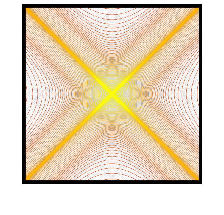 |
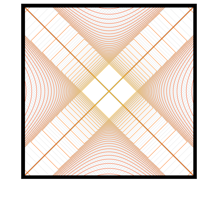
| (a) Lines of constant tortoise coordinate | (b) Lines of constant radius |
 |
 |
| (c) Lines of constant tortoise coordinate | (d) Lines of constant radius |
 |
 |
 |

|
 |

|
 |

|
Appendix A Comparison to existing methods
The method described in this article generalizes and unifies techniques from various sources. In order to provide the proper context, we conduct here a brief review of the methods historically used to create similar diagrams.
The problem of generating causal diagrams for SSS spacetimes has previously been tackled in two fundamental ways: the method of block diagrams and the method of global Penrose coordinates. The block diagram method provides explicit global Penrose coordinates only when the metric function has one or zero horizon radii (locations where ). When many horizons are present, the block diagram method allows qualitative analysis by the identification of overlapping blocks in neighboring quad-block regions (see section 4), but does not define a self-consistent system of global coordinates in the area of overlap.
The more well known of the two methods is that of block diagrams, in which the causal structure of spacetime is pieced together from quad-block units. This method was first applied to the special case of Schwarzschild spacetime by Kruskal [19]. Maximally extended Schwarzschild spacetime, with its one horizon radius, consists of a single quad-block, and so in this case global Penrose coordinates were also achieved. Kruskal’s method was then generalized by Walker to the method of block diagrams [4]. In Walker’s treatment, quad-blocks could be constructed so long as the metric function took a special form, with the tortoise function defined by an indefinite integral (although definite integrals were implemented to generate the tortoise function within individual blocks). Later, however, Brill and Hayward [20] used a definite integral formulation to extend Walker’s method to the case of an arbitrary metric function, in a manner equivalent to the results of section 4.5. In this way, the question of constructing arbitrary block diagrams (but not Penrose diagrams) for SSS spacetimes has long since been settled.
The less well known set of methods is that in which global Penrose coordinates are explicitly constructed. The most important progress in this direction was made by Carter [3], who found global Penrose coordinates for special cases with two horizons. Although Carter’s method relied on the ability to determine the tortoise function by an indefinite integral, and assumed the existence of exactly two horizons, it is in fact easily generalizable, and was the most important contribution to the present methods. In fact, when the indefinite integral form of the tortoise function is known, Carter’s two-horizon method is essentially equivalent to the method of section 5, but with the substitution in every block. The original Carter method does have several drawbacks. One is that the exponential form of yields very strange-looking lines of constant radius (see figure 19). Additionally, applied to a case with more than two horizons, this method would suffer from major problems near the undefined radius points (see section 4.7), and need to be modified. The results of section 5 can be thought of as a generalization of the methods of Carter; the key new additions are the introduction of the global tortoise function and the new form of the function . These additions allow the method to be extended to an arbitrary metric function with an arbitrary number of horizons, while simultaneously rendering the diagram more readable.
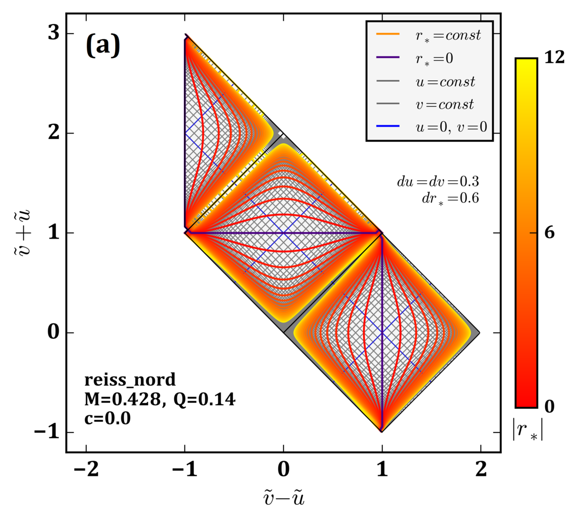 |
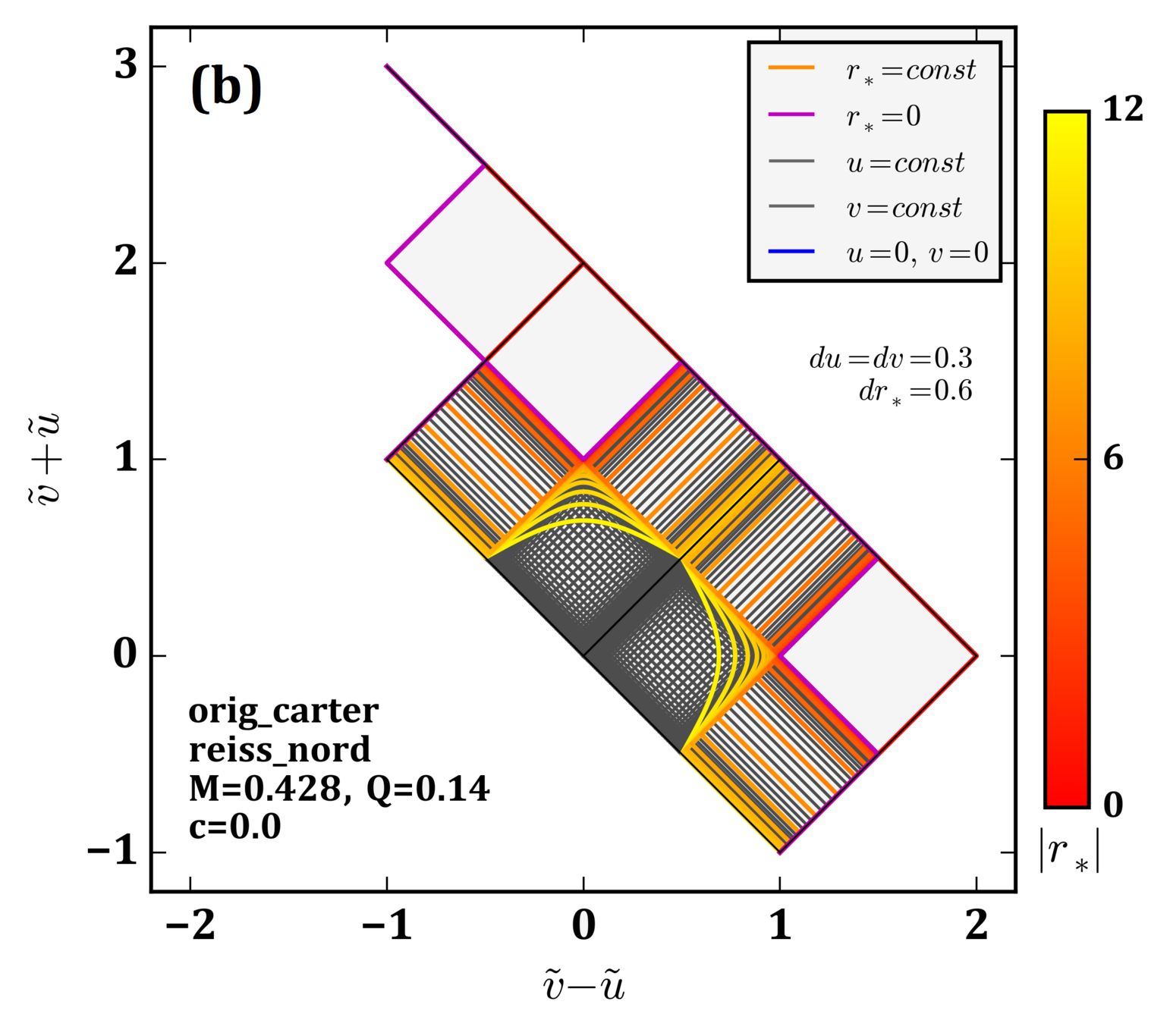 |
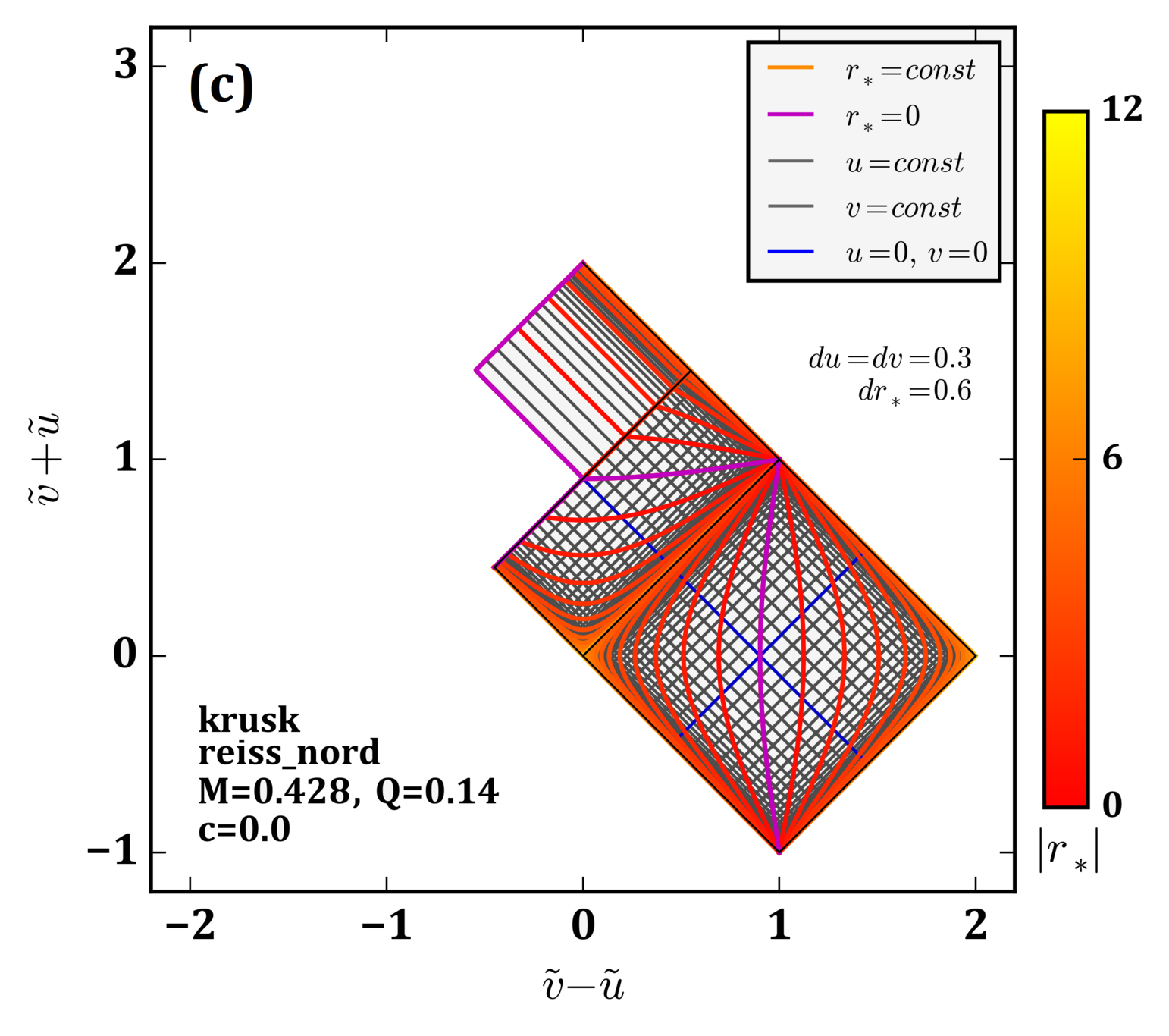 |
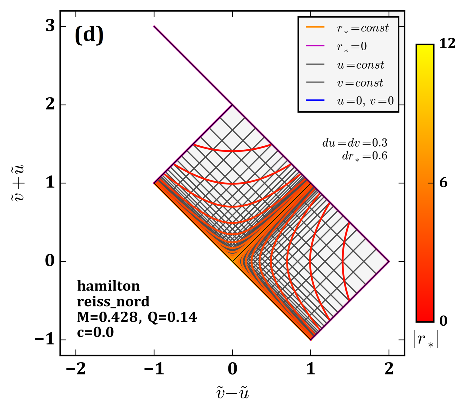 |
In order to understand the advantages of the present method, it is useful to compare the known methods for constructing Penrose diagrams in the case of two horizons. Such a comparison is depicted in figure 19. Once the tortoise function is set and the double-null coordinates are defined in each block, there are several known methods of obtaining the diagram coordinates. First, of course, there is the method of section 5. Second, there is the original method of Carter [3]. Both have been described above. A third method has been used by Hamilton [6]; this method could potentially also be generalized, but is less theoretically appealing than Carter’s method. Finally, it is possible to define a two-horizon extension of the Kruskal method such that the diagram matches the standard Kruskal diagram outside of some inner limit; this two-horizon Kruskal-like method cannot be extended to more horizons, however, and so although it is shown for comparison, we omit its exact formulation. In figure 19, diagrams featuring lines of constant tortoise coordinate are shown for each of these four methods. Showing the tortoise coordinate instead of radius isolates the effect of the different coordinates systems, eliminating distortion due to .
Appendix B Unit conventions
A major goal of the techniques described in this article is to realize Penrose diagrams of physically relevant spacetimes. As such, we must clarify the status of units in these calculations. First of all, note that we utilize standard conventions for geometrized units, such that , in accordance with [21, (Appendix F)]. The tricky issue of units in the coordinates, metric components, and Penrose diagrams is discussed below.
In GR the units of the line element are necessarily . Units for other geometric quantities depend on a choice of convention. Among the possible conventions, there is a unique simplest choice: all metric components should be unitless, while all coordinates carry units of length. This convention has several benefits. All components of a tensor have the same units. The components of an even-rank tensor have the same units as its scalar contractions. And for any given tensor, the covariant, contravariant, and mixed varieties all have the same units. In particular the Ricci curvature components and Ricci scalar obey , and after conversion to SI units by all components of the stress-energy tensor have units (where is the number of spacetime dimensions). There are other standard unit conventions in which these need not hold. For example in the standard Euclidean spherical coordinates where and , the components do not even all have the same units.
We achieve this simplest convention while maintaining notational simplicity by factoring out and suppressing a universal length scale. Let the physical line element have any arbitrary unit convention such that . Let be an arbitrary length scale. It is always possible to nondimensionalize the coordinates and metric components to obtain with , where . Then the physical line element can always be expressed as in terms of the unitful coordinates and the unitless metric. This form of the physical line element satisfies the desired convention.
We will always write the unitless line element in the unitless coordinates as a shorthand for the true line element in the unitful coordinates , never making the arbitrary length scale explicit. Note that derivatives pick up an extra factor of the length scale when calculating in the shorthand. By keeping track of these and similar factors, one can easily relate geometric quantities in the unitful geometry to those in the unitless geometry.
Additionally, all parameters in the metric components are by convention unitless. Any physical, unitful, parameters must be obtained by studying the resultant geometry of the physical metric .
Consider the demonstrative example of three dimensional Euclidean flat space in spherical coordinates. We write this geometry in the unitless shorthand coordinates , with line element . This serves as shorthand for the the unitful coordinates , and the unitful metric , with and .
Moreover, to see how parameters in the metric correspond to physical parameters, consider for example the Schwarzschild metric , as expressed here in the unitless shorthand coordinates. The parameter is unitless. By inspection of the geometry , one finds that the physical Schwarzschild radius is , and the physical Schwarzschild mass in SI units is .
The Penrose diagrams we construct are for the unitless metric . The Penrose coordinates are unitless, and in all examples no absolute length scale appears in the metric components. Consequently, the appearance of the Penrose diagrams never depends on the arbitrary length scale factor. To return to units, one simply notes that if are Penrose coordinates for , then are Penrose coordinates for . Once the length scale is set, all lengths are defined in units, and other geometrical quantities must be calculated in units as described above.
Appendix C Spherical symmetry with a fixed origin
To properly describe SSS spacetimes requires the concept of spherical symmetry about a fixed origin. Since manifolds need not contain their symmetry axes, this requires a bit of extra work.
To set the stage, let us recall some facts about the symmetry of psuedo-Riemannian manifolds (i.e. metric manifolds of arbitrary signature). Such a -dimensional manifold usually has a continuous (Lie) group of isometries. Continuous isometries are generated by flow along Killing vector fields, which satisfy . The set of Killing vector fields, under the Lie bracket operation, form a Lie algebra equivalent to that of . The maximum number of independent Killing vector fields (maximum dimension of ) is always . Spaces saturating this maximum are maximally symmetric, have constant curvature, and are homogenous and isotropic, at least locally [22]. In particular the -sphere , with metric induced from Euclidean space, is a maximally symmetric space of positive curvature. The isometry group of is the orthogonal group , defined as the Lie group of real orthogonal matrices. The corresponding Lie algebra , defined as the real algebra of real antisymmetric matrices, has dimension . It is by analogy with this symmetry algebra that we define spherical symmetry in spacetime.
Let be a spacetime of dimension . is called -spherically symmetric if (i) the Lie algebra of Killing vector fields of has a spacelike subalgebra isomorphic to , such that (ii) the local dimension of as a subspace of is either or at each point . In general there may be many such subalgebras , each corresponding to a different symmetry axis. Therefore we will call a choice of one specific a choice of the origin of spherical symmetry, and the pair an -spherically symmetric spacetime with fixed origin (but we will abuse notation and simply refer to , with implied).
Now suppose is -spherically symmetric with origin fixed by . Points where the local dimension of is 0 are fixed points of the spherical symmetry; we call the set of all such points the axis . The axis may be empty or nonempty. When nonempty, it is typically a dimensional submanifold of . The complement of the axis we shall denote . By assumption, has local dimension on . Thus by Frobenius’s theorem [23], is foliated by -dimensional integral submanifolds of corresponding to isometric flows along . Each point is contained in exactly one such submanifold, called its orbit and denoted .
We wish to show that each of these orbits has the intrinsic geometry of a sphere (its intrinsic geometry being induced by the metric on ). We do so by determining Killing vectors of the orbits. Each Killing flow generates an isometry of , which in turn induces an isometry on the invariant subspace . Since additionally is tangent to the orbits, is an algebra of Killing vector fields on the orbit, and the vector field commutators of are preserved by the restriction. One could imagine, however, that when restricted to the orbit, may no longer have the same number of independent generators (i.e. if two linearly independent fields, when restricted, became linearly dependent). This possibility is mostly (i.e. for ) ruled out by the group theoretic considerations of [24]. A more concise proof follows from the algebraic approach, as follows. The restriction , being both linear and commutator-preserving, defines a Lie algebra homomorphism. The kernel of the homomorphism must be an ideal. But since simple Lie algebras have no nontrivial proper ideals, and since our assumption on the local dimension of implies that , simplicity of implies that . Thus, whenever is simple, leaving only the cases and [25]. The same dimensionality holds for the case , since in that case already. Let us assume the case causes no problems.
The above reasoning shows that restricts to a spacelike dimensional algebra of Killing vector fields on the -dimensional orbits, so it follows that each orbit is a maximally symmetric Riemannian manifold with symmetry algebra isomorphic to . This implies that each orbit must be locally isometric to the sphere with metric . It is therefore justified to define the areal radius (relative to ) at each point by . Correspondingly, for points on the symmetry axis we define . In this way the areal radius is defined for all points in .
At every point not on the symmetry axis, there exists a local coordinate system exhibiting the foliation by spheres. Let . Then has a neighborhood with coordinates , in which the metric reads
| (35) |
where is a -dimensional Lorentzian metric depending only on , the coordinates parameterize a -orbit for fixed , and is the areal radius of such an orbit. For each point with coordinates in this patch, . That such a coordinate system exists can be shown by construction of surface-orthogonal geodesic coordinates [26]; another proof is given by [27, (s. 13-5)].
Let it be emphasized: once an origin of spherical symmetry is fixed by choosing , the areal radius is an intrinsic property of each point , independent of coordinate system. is foliated by spheres (lying tangent to ) with intrinsic metric , except on the axis of symmetry where by definition. Everywhere except on the axis, there is a local coordinate system respecting this foliation, in terms of which the metric is (35).
Appendix D Proof of regularity at the horizons
Here we prove that the Penrose-coordinate metric coefficients are continuous and nonzero at all horizons and horizon vertices in Penrose diagrams obtained by the methods of section 5. The only exception is that the metric is sometimes discontinuous at horizon points in a small neighborhood near , in non-vertex corners of the diagram, as described in section 4.7. Before proceeding, properties of the global tortoise function of section 5 are proved, and some useful identities are developed.
Properties of the Global Tortoise Function
The identities (14) and (15) are proved by showing that for each zero of there exists a cut punctured disk about the origin in the complex plane, and a function analytic at , such that for on the real axis in ,
| (36) |
It follows that the complex function is analytic at , which, as seen below, quickly implies the desired results.
The proof of (36) runs as follows. Denote , where is the defining integral in (11) with the real part sign removed. Evaluation of the semicircular contours in the small limit shows that . By assumption, is complex analytic at with and . Power series arguments show that there exists a (as above) on which
| (37) |
with analytic at and , and on which is analytic with analytic antiderivative
| (38) |
where is also analytic at . , which can be written as a constant plus an integral contained in , analytically extends to the antiderivative for a suitable constant. Comparing imaginary parts in for on the real axis shows that with . Thus .
Useful identities
Here we collect some useful identities for the functions and , and the coordinate transformations and , of section 5.2. The identities below include some inverse functions, which are useful for determining radii of points in the diagram, and some derivative identities, which are useful for analysis of the metric.
First of all, there are the inverse functions
| (40) |
| (41) |
which must be used to determine radii of points in the diagram.
Meanwhile, the derivatives we want are
| (42) |
| (43) |
From the derivatives one observes that .
Now denote . Due to the piecewise nature of this function, it is useful to also define the piecewise constant
| (44) |
In this notation (and suppressing the argument), one can write the simple expressions
| (45) |
| (46) |
| (47) |
Let be a joint notation for and . For both and , the transformation from block to Penrose coordinates has the general form
| (48) |
for real constants , where is monotonic increasing. It follows that is monotonic and invertible, and the derivative is
| (49) |
Applying (46) and (47) with (48) and (49), one obtains
| (50) |
with , wherever (and again, represents either or ).
All necessary identities are now in hand.
Proof of regularity
We shall demonstrate that, in the Penrose coordinates , the metric coefficients are continuous and nonzero in the coordinate basis at horizons and horizon vertices, except possibly in arbitrarily small corners of the diagram where , , and . The proof proceeds by direct calculation of the metric components in a neighborhood of horizon points.
As usual (see section 4.2), suppose that is a shorthand representing either or . Begin with metric coefficients written in the form (23). In order to evaluate the metric at , one sets the free parameter . The function (14), which carries the explicit radial dependence, was already shown to be analytic (and thus continuous) and positive at . All that is left is to evaluate the functions and in the appropriate limits. The details run as follows.
In light of (50), the metric coefficients (24-25) in each block can be rewritten
| (51) |
| (52) |
where and , utilizing the notation (44).
Now suppose there are multiple blocks, all matched to their neighbors according to the prescription of section 5.3. Further, suppose without loss of generality that one of the blocks has the parameters . Since all blocks must have been shifted by integer values of , it follows from the periodicity that in every block the metric coefficients are
| (53) |
| (54) |
All metric dependence on the shift parameters has been eliminated.
It remains to implement the limit . In any block bordering a horizon radius , it is easy to see from their definitions that the coordinate limits have a standard pattern, depending on the sign of . Suppose that . Then in any block bordering , one finds and and . As a result, one finds the important result that as , either , or , or both. By using the free parameter , the limiting value can now be evaluated.
Suppose that two blocks and are joined along a line of constant , as in section 5.3. In both blocks, near the horizon, and the limits of the preceding paragraph are such that . Then letting , one finds
| (55) |
which obtains the limit
| (56) |
when , since there. The limit (56) is independent of block parameters, and thus automatically equal in both blocks, ensuring that is positive and continuous across the horizon.
Meanwhile, at horizon points, the coordinate parameterizing the horizon remains finite. On the horizon, the corresponding metric factor becomes
| (57) |
where corresponds to and respectively. This expression holds on both sides of the horizon, in both blocks and , and is strictly positive. Since the matching conditions ensure that , the function (57) is equal on both sides of the horizon for all such that (which also implies ). Near horizon vertices, where all transformations have the same exponential factor, and in the bulk of blocks, where , this matching is guaranteed. However, when both and near , then may be different in the neighboring blocks for the relevant direction, yielding a discontinuity. By choosing large, the neighborhood affected by this is exception may be made arbitrarily small. Thus at all horizon points, except near , the function is positive and continuous across the horizon. At a horizon vertex point, the limit (56) applies to both and , for all surrounding blocks, and the metric is, again, continuous.
To summarize, utilizing (55) and (57), the metric in a neighborhood of any horizon point or vertex point at can be written
| (58) |
Every factor in the coefficient of has by been shown to be positive and continuous as a function of in this neighborhood, except in arbitrarily small neighborhoods where . Thus, except for the polar coordinate singularity at , and except for the above-noted exception, the global metric is continuous and strictly positive everywhere. Our goal of obtaining non-degenerate continuous global Penrose coordinates extending across an arbitrary number of horizons has been achieved.
Given the analyticity of the radial dependence in the metric (see (14)), one might hope to give a coordinate system which extends the full metric analytically across horizons. Indeed, this is possible by simply choosing a suitable . However, a trade-off has to be made. If analyticity at the horizons is retained, either differentiability of the interior metric, simplicity of , or simplicity of the diagram appearance must be sacrificed. An example of the latter case may be seen in figure 19(b). Since there is no physically motivated benefit to retaining analyticity, we give it up.
Appendix E More properties of SSS spacetimes
For convenience, we collect here some geometrical formulae for a four-dimensional SSS spacetime. Let the metric function be written
| (59) |
We imply no restriction whatsoever on the function . This is simply a very useful way to write the metric function. It is only sometimes appropriate to interpret as the total mass inside radius . Useful derived quantities include the shell mass
| (60) |
(see (63) and below) which determines the Einstein tensor, and the function
| (61) |
which controls the Weyl tensor.
Orthonormal basis
We define an orthonormal basis in each block. Where define and . Where define and . And, everywhere, define and . In this construction is always timelike. Both and can be continuously extended across horizons, which is why the Einstein tensor in this basis (below) will have no discontinuities associated with the piecewise definition. However the basis cannot be continuously extended, as the extensions of and would coincide at the horizon. Despite this shortcoming, we often choose to work in this basis for its conceptual and calculational simplicity.
Curvature components in coordinate bases
These quantities were computed with help from the Mathematica package RGTC [28]. Sign conventions for the curvature tensors are equivalent to those found in Wald [21].
In the coordinate basis, the nonzero Christoffel symbols are and and and and and .
The Riemann tensor has the symmetries and and [7]. Using the symmetries, all nonzero components of are generated in the coordinate basis by and and and , where and .
The Weyl tensor has the same symmetries as the Riemann tensor above. Using the symmetries, all nonzero components of are generated in the coordinate basis by and and and , where and .
For calculations involving null curves and surfaces, it is often useful to also know the covariant derivative in null coordinate systems.
In double null coordinates with metric , the relevant Christoffel symbols can be evaluated by the chain rule on and . The nonzero components are and and and and and .
Meanwhile, in the EF coordinate basis (with metric (3)), the nonzero Christoffel symbols are, by direct computation, and and and and and and .
Matter content, curvature scalars, and energy conditions
The Einstein tensor in the orthonormal basis (defined above) is given by
| (62) |
where
|
(63) |
Thus, may always be interpreted as proportional to the mass of a thin shell at radius . When is constant, density diffuses naturally as , and there is no transverse pressure.
The curvature scalars are
| (64) |
| (65) |
| (66) |
| (67) |
The basis diagonalizes , with one timelike and three spacelike eigenvectors. The corresponding eigenvalues are the negative of the density (timelike) and the principal pressures (spacelike). It is well known that in this case, the classical energy conditions take on simple forms [5]. In particular, the null energy condition amounts to . For us, always, and the remaining NEC constraint is equivalent to . The weak energy condition amounts to the NEC plus the constraint , which for us becomes . The flux energy condition of [29] amounts to in the diagonalized case. Again, the SSS case trivially saturates , and the remaining constraint is equivalent to .
Trapped surfaces
A closed spacelike surface is called future trapped (past trapped) if its mean curvature vector is everywhere future-directed timelike (past-directed timelike) on [14]. In this expression, the are future-directed null vectors, each orthogonal to , normalized by . The are the corresponding future null expansions; they can be defined by , where is a basis on the tangent space of , and is the inverse of the induced spatial metric on .
In an SSS spacetime, the sphere , contained within a block , is a closed trapped surface if and only if . This is proved by direct calculation of the mean curvature vector of the sphere at SSS block points. It is simplest to work in double-null block coordinates , in terms of which the metric is (7). Since is a surface of constant coordinates, its tangent space is spanned by the coordinate basis and , and the induced metric has line element . A pair of mutually normalized null vectors orthogonal to is given by and . With this setup, the expansions simplify to . Thus we obtain and . The mean curvature is timelike if and only if , which implies that is trapped if and only if . Additionally, it is always true that . Thus when is trapped, is future-trapped (past-trapped) if and only if as defined above are both future-directed (past-directed). This completes the proof of the desired result.
Cartesian coordinates near the origin
In a neighborhood of (contained in ), one can naively make the transformation from into the cartesian coordinates , according to the standard spherical coordinate transformation, such that . The metric becomes
| (68) |
which can be used to study the limit as , as seen below.
Singularity
The metric may be either singular or nonsingular at the origin. If has a Laurent series expansion about then the following are equivalent:
-
1.
is called nonsingular at the origin;
-
2.
as ;
-
3.
as ;
-
4.
Curvature scalars , , , all finite at origin;
-
5.
Cartesian metric has a finite limit as ;
-
6.
contains the axis as a set of points, and is geodesically complete there
(i.e. all geodesics terminating there can be extended);
Proof. By definition , and trivially . Direct calculation shows and . Then and by existence of normal neighborhoods [30], assuming sufficient differentiability.
Evidently if an SSS spacetime is nonsingular at the origin, then , the axis is a timelike curve, and to quadratic order the dominant behavior as is either flat, de Sitter, or Anti de Sitter.
References
References
- [1] R. Penrose. Republication of: Conformal treatment of infinity. General Relativity and Gravitation, 43:901–922, March 2011.
- [2] R. Penrose. Zero rest-mass fields including gravitation: Asymptotic behaviour. Proceedings of the Royal Society of London A: Mathematical, Physical and Engineering Sciences, 284(1397):159–203, 1965.
- [3] Brandon Carter. Complete analytic extension of the symmetry axis of kerr’s solution of einstein’s equations. Phys. Rev., 141:1242–1247, Jan 1966.
- [4] Martin Walker. Block Diagrams and the Extension of Timelike Two-Surfaces. Journal of Mathematical Physics, 11(8):2280–2286, 1970.
- [5] S. W. Hawking and G. F. R. Ellis. The Large Scale Structure of Space-Time (Cambridge Monographs on Mathematical Physics). Cambridge University Press, 1973.
- [6] Andrew J.S. Hamilton. General Relativity, Black Holes, and Cosmology. Unpublished. Online at http://jila.colorado.edu/~ajsh/astr3740_17/grbook.pdf.
- [7] Jerry B Griffiths and Jiří Podolskỳ. Exact space-times in Einstein’s general relativity. Cambridge University Press, 2009.
- [8] Sean A. Hayward. Formation and evaporation of nonsingular black holes. Phys. Rev. Lett., 96:031103, Jan 2006.
- [9] R. Geroch, E. H. Kronheimer, and R. Penrose. Ideal points in space-time. Proceedings of the Royal Society of London A: Mathematical, Physical and Engineering Sciences, 327(1571):545–567, 1972.
- [10] Piotr T. Chrusciel, Christa R. Olz, and Sebastian J. Szybka. Space-time diagrammatics. Phys. Rev., D86:124041, 2012.
- [11] John C. Graves and Dieter R. Brill. Oscillatory character of reissner-nordström metric for an ideal charged wormhole. Phys. Rev., 120:1507–1513, Nov 1960.
- [12] Robert M. Wald. The thermodynamics of black holes. Living Reviews in Relativity, 4(1):6, 2001.
- [13] Jose M. M. Senovilla. Trapped surfaces. Int. J. Mod. Phys., D20:2139, 2011.
- [14] Ingemar Bengtsson and Jose M. M. Senovilla. The Region with trapped surfaces in spherical symmetry, its core, and their boundaries. Phys. Rev., D83:044012, 2011.
- [15] C. Barrabès and W. Israel. Thin shells in general relativity and cosmology: The lightlike limit. Phys. Rev. D, 43:1129–1142, Feb 1991.
- [16] Tevian Dray and Gerard ’t Hooft. The effect of spherical shells of matter on the schwarzschild black hole. Communications in Mathematical Physics, 99(4):613–625, Dec 1985.
- [17] Ian H. Redmount. Blue-sheet instability of schwarzschild wormholes. Progress of Theoretical Physics, 73(6):1401, 1985.
- [18] C. Barrabès and P. A. Hogan. Singular Null Hypersurfaces in General Relativity: Light-Like Signals from Violent Astrophysical Events. World Scientific Publishing Co, 2003.
- [19] M. D. Kruskal. Maximal extension of schwarzschild metric. Phys. Rev., 119:1743–1745, Sep 1960.
- [20] Dieter R Brill and Sean A Hayward. Global structure of a black hole cosmos and its extremes. Classical and Quantum Gravity, 11(2):359, 1994.
- [21] Robert M Wald. General relativity. Chicago Univ. Press, Chicago, IL, 1984.
- [22] Walter Thirring. A Course in Mathematical Physics 1 and 2: Classical Dynamical Systems and Classical Field Theory. Springer, 1992.
- [23] Bernard F. Schutz. Geometrical Methods of Mathematical Physics. Cambridge University Press, 1980.
- [24] Deane Montgomery and Hans Samelson. Transformation groups of spheres. Annals of Mathematics, 44(3):454–470, 1943.
- [25] Brian C. Hall. Lie Groups, Lie Algebras, and Representations: An Elementary Introduction (1st Ed.). Springer, first edition, 2003.
- [26] Sean Carroll. Spacetime and Geometry: An Introduction to General Relativity. Pearson, 2003.
- [27] S. Weinberg. Gravitation and Cosmology: Principles and Applications of the General Theory of Relativity. July 1972.
- [28] S. Bonanos. Capabilities of the Mathematica Package ’Riemannian Geometry and Tensor Calculus’. In K. D. Kokkotas and N. Stergioulas, editors, Recent Developments in Gravity, pages 174–182, 2003.
- [29] Prado Martín-Moruno and Matt Visser. Semiclassical energy conditions for quantum vacuum states. Journal of High Energy Physics, 2013(9):50, 2013.
- [30] Barrett O’Neill. Semi-Riemannian Geometry With Applications to Relativity. Academic Press, 1983.